Complete characterization of the macroscopic deformations of periodic unimode metamaterials of rigid bars and pivots.

To begin with we mainly concentrate on trajectories $(\lambda_{1}(t_{0}),\lambda_{2}(t_{0}))$ for which $\lambda_{2}$ is a single valued continuous function $\lambda_{2}=f(\lambda_{1})$ of $\lambda_{1}$. As we will see there are many operations that can be done with realizable functions to obtain new realizable functions. We will not cover all of them, only those necessary to establish the main result of the paper, that all trajectories are approximately realizable. We start with the elementary (and obvious) ones,

• •

  Rescaling: If $\lambda_{2}=f(\lambda_{1})$ is realizable then so is $\lambda_{2}=\alpha^{-1}f(\alpha\lambda_{1})$, for any real constant $\alpha>0$, by rescaling the microstructure in the cell.

• •

  Rotation: If $\lambda_{2}=f(\lambda_{1})$ is realizable then so is $\lambda_{1}=f(\lambda_{2})$ by rotating the cell (and its microstructure) by $90^{\circ}$. This is most useful when $\lambda_{2}$ is a vertical distance which determines the horizontal distance $\lambda_{1}$ though the function $f$.

• •

  Reshaping: If $\lambda_{2}=f(\lambda_{1})$ is realizable and $f$ is continuous, $\lambda_{2}=rf(\lambda_{1})$ is realizable for any rational $r=p/q$, where $p$ and $q$ are integers. To see this, for simplicity in the case where $p=3$ and $q=2$, consider an array of $np$ cells in the vertical direction and $nq$ cells in the horizontal direction, as illustrated in figure 4 with $n=4$, where the bipod supports have leg length $d$ (and have a pivot joint at the midpoint). By rescaling the microstructure of the material we can assume $g=(nq)^{-1}f(nqh)$. Also let the bipod supports scale as $d=d_{0}/\sqrt{n}$, so they are small compared with $\lambda_{1}$ and $\lambda_{2}$ but large compared with the cell size. Then as $n\to\infty$ we have $nqh\to\lambda_{1}$ and $npg=rf(nqh)\to\lambda_{2}$. So in the limit we see that $\lambda_{2}=rf(\lambda_{1})$.

• •

  Addition: If $\lambda_{2}=f_{1}(\lambda_{1})$ and $\lambda_{2}=f_{1}(\lambda_{1})$ are both realizable and continuous, then $\lambda_{2}=f_{1}(\lambda_{1})+f_{2}(\lambda_{1})$ is realizable. Referring to figure 5, illustrated for the case $n=8$, by rescaling the microstructure of the material we can assume $g_{1}=(n)^{-1}f_{1}(nh)$ and $g_{2}=(n)^{-1}f_{2}(nh)$. We again let the supports scale as $d=d_{0}/\sqrt{n}$. Then as $n\to\infty$ we have $nh\to\lambda_{1}$ and $ng_{1}+ng_{2}=f_{1}(nh)+f_{2}(nh)\to\lambda_{2}$. In the limit we obtain $\lambda_{2}=f_{1}(\lambda_{1})+f_{2}(\lambda_{1})$.

We obviously need some elementary realizable functions to begin building more complicated ones. Let us examine in more detail the response of the expander of figure 2(c). The unit cell is shown in more detail in figure 6(a), which defines various parameters. Elementary trigonometry shows that

implying that $(\lambda_{1},\lambda_{2})$ lies on the portion of the ellipse

with $2\sqrt{\varepsilon^{2}+a^{2}}>\lambda_{1}>2\varepsilon$ and $2a>\lambda_{2}>2a\varepsilon/\sqrt{\varepsilon^{2}+a^{2}}$ where the last constraint ensures that the triangles remain in the cell.

In particular let us take $n$ of these elements, arranged as in figure 6(b), to form a new cell with dimensions $(\lambda_{1}^{\prime},\lambda_{2}^{\prime})$ and let us set $\varepsilon=\varepsilon_{0}/n^{2}$ and $d=d_{0}/n^{2}$ keeping $a$ independent of $n$. Then given a domain $D$ of operation, $\lambda_{1}^{-}<\lambda_{1}^{\prime}<\lambda_{1}^{+}$, we choose $n$ sufficiently large that the minimal extension of the expander is less than $\lambda_{1}^{-}$ and its maximum extension is greater than $\lambda_{1}^{+}$. Then for any given $\lambda_{1}^{\prime}$ in $D$ we have

These estimates in conjunction with (2.2) imply that for any $\lambda_{1}^{\prime}$ in $D$, $\lambda_{2}^{\prime}$ converges to $2a$ as $n\to\infty$, independent of $\lambda_{1}^{\prime}$. In other words any positive constant function is (approximately) realizable on a given domain $D$. Such a cell behaves like an ideal expander: when $n$ is very large we can adjust the horizontal length as we please (within the domain $D$) and the vertical length remains (essentially) unchanged. From a practical viewpoint we caution that the structure will likely be very sensitive to small imperfections when $n$ is large.

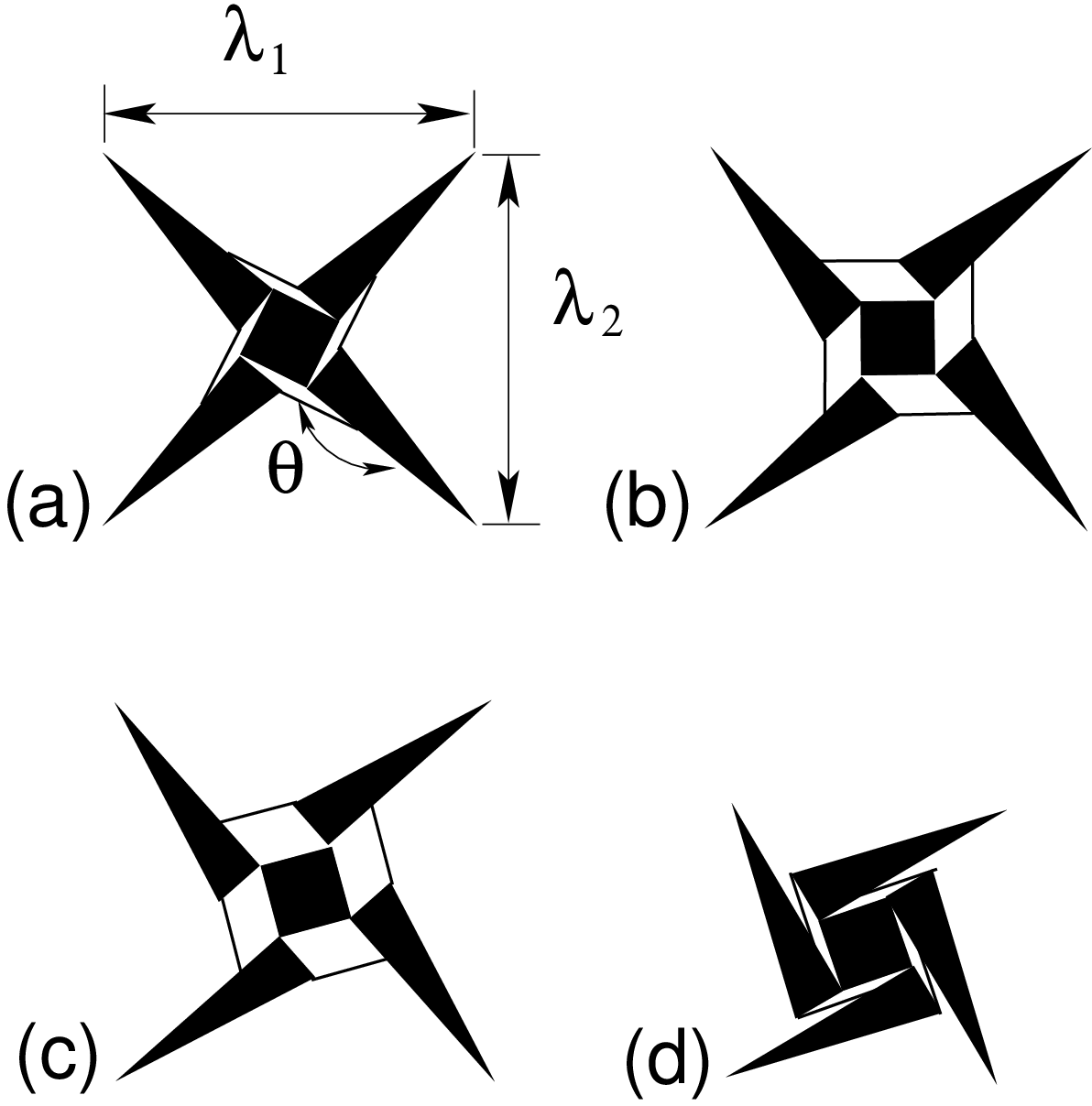
Another important cell is a dilator. An example of one, based on the chiral geometries of [Milton (1992)], [Prall and Lakes (1996)], and [Mitschke et al. (2011)], is shown in figure 7 in four states of deformation. If the innermost square has side length $\ell$ and the right angled triangle has height $h$ and base $b<\ell$, then the cell dimensions are

having a minimum value of

at $\theta=0$ and a maximum value of

at $\theta=3\pi/4$ corresponding to case $(b)$ in figure 7. We call $(t_{0}^{-},t_{0}^{+})$ the performance range of the dilator. Rescaling the microstructure allows us to get performance ranges $(kt_{0}^{-},kt_{0}^{+})$ for any constant $k>0$.

Now by combining four expanders with this basic dilator cell, as sketched in figure 8, one can obtain dilators having an arbitrarily large performance ratio $t_{0}^{+}/t_{0}^{-}$ of maximum extension to minimum extension. To see this, suppose each expander has $n$ unit cells and let the dimensions of the inner basic dilator scale as $\ell=\ell_{0}/n$, $h=h_{0}/n$ and $b=b_{0}/n$, let the dimensions of the expander scale as $a=a_{0}/n$, $\varepsilon=\varepsilon_{0}/n^{2}$, and let the dimensions of the bipod supports scale as $d=d_{0}/n$. Choose $a_{0}$ in the range

so that the inner basic dilator can never reach its maximum extension, but the expander can attain its minimal extension at $\alpha=0$ and can have an angle $\alpha$ at least as large as $45^{\circ}$. (This inequality implies $\ell_{0}$ and $h_{0}$ must be chosen with $6h_{0}\ell_{0}>2h_{0}^{2}+\ell_{0}^{2}$ as may be satisfied with $h_{0}=\ell_{0}$, for example). Choose $d_{0}>\sqrt{2}a_{0}$ so that the microstructure is always contained in the cell. When the expanders are fully compressed they have a length of $2n\varepsilon=2\varepsilon_{0}/n$, and since the maximum possible dimensions of the inner basic dilator scale as $1/n$ and the supports scale as $1/n$ it follows that the minimum extension scales as $1/n$. By contrast with $\alpha=45^{\circ}$ the expanders have an extension of $\sqrt{2}a_{0}$ in the limit $n\to\infty$. Therefore the performance ratio of maximum extension to minimum extension can be as large as one pleases with this microstructure by choosing $n$ large enough. Thus the function $\lambda_{2}=\lambda_{1}$ is realizable, and by addition with an ideal expander so is the function $\lambda_{2}=\lambda_{1}+c$ for any constant $c>0$.

Now that we have dilators we can build many things.

• •

  To build a material where in a domain $\lambda_{2}$ depends linearly on $\lambda_{1}$ with negative slope consider the microstructure of figure 9. In the cell there are $n$ dilator cells in the horizontal direction and $n$ dilator cells in the vertical direction. We only show one corner of the cell as the microstructure in the other corners are just reflections of this microstructure about the $x_{1}$ and $x_{2}$ axes. We scale the geometry with $a=a_{0}/\sqrt{n}$, $b=a_{0}/\sqrt{n}$, $c=c_{0}/\sqrt{n}$, $d=d_{0}/\sqrt{n}$, and $\phi=\phi_{0}/\sqrt{n}$ while varying $\theta$ so that $\theta+\phi$ is independent of $n$. Since by trigonometry $\alpha+\gamma+\theta=\pi$ and $\theta+\phi+\gamma-\beta=\pi$ we deduce that $\alpha+\beta=\phi=\phi_{0}/\sqrt{n}$. So as one might expect, the angles $\alpha$ and $\beta$ must go to zero as $n\to\infty$. We can let $\alpha=\alpha_{0}/\sqrt{n}$ and $\beta=\beta_{0}/\sqrt{n}$ where $\alpha_{0}>0$ and $\beta_{0}>0$ depend on the deformation and $\alpha_{0}+\beta_{0}=\phi_{0}$. Then the length $nh$ of the dilator segment in the horizontal direction satisfies

  $$nh=2nb\sin{\alpha}=2\sqrt{n}b_{0}\sin{(\alpha_{0}/\sqrt{n})}\to 2b_{0}\alpha_{0}\quad{\rm as}~n\to\infty,$$

  (2.8)

  while the length $ng$ of the dilator segment in the vertical direction satisfies

  $$ng=2nc\sin{\beta}=2\sqrt{n}c_{0}\sin{(\beta_{0}/\sqrt{n})}\to 2c_{0}\beta_{0}\quad{\rm as}~n\to\infty.$$

  (2.9)

  We restrict the range of operation so $\lambda_{1}>\eta$ and $\lambda_{2}>\eta$ for some small $\eta>0$. Then $(\lambda_{1},\lambda_{2})$ must approach $(nh,ng)$ since the corner cell geometry scales roughly as $1/\sqrt{n}$. Finally since $\alpha_{0}+\beta_{0}=\phi_{0}$ we conclude that, in the limit $n\to\infty$,

  $$\lambda_{2}=2c_{0}\phi_{0}-(c_{0}/b_{0})\lambda_{1}.$$

  (2.10)

  Since the ratio $c_{0}/b_{0}$ can be any positive value we please, it is clear that we can get any negative slope. By rescaling it is clear that the constant can take any desired positive value.

  

• •

  To build a material where in a domain $D$, $0<\lambda_{1}^{-}<\lambda_{1}<\lambda_{1}^{+}$, $\lambda_{2}$ depends quadratically on $\lambda_{1}$ consider the microstructure of figure 10. In the cell there are $n^{2}$ dilator cells in the horizontal direction and $n^{3}$ dilator cells in the vertical direction. Like in the previous example we only show one corner of the cell as the microstructure in the other corners are just reflections of this microstructure about the $x_{1}$ and $x_{2}$ axes. Since $a$ and $b$ are sides of a triangle with opposite angles $\beta$ and $\pi/2-\alpha$ the law of sines implies $\sin\beta=(a/b)\cos\alpha$. To ensure that $\gamma=0$ when $\alpha=0$, in which case $\beta=\theta$, we choose $\sin\theta=a/b$. Then we have

  	$\displaystyle g$	$\displaystyle=$	$\displaystyle 2c\sin\gamma=2c\sin(\theta-\beta)$		(2.11)
  		$\displaystyle=$	$\displaystyle 2c\left[\sin\theta\sqrt{1-(a/b)^{2}\cos^{2}\alpha}-(a/b)\cos\theta\cos\alpha\right]$
  		$\displaystyle=$	$\displaystyle(2ca/b)\left[\sqrt{1-(a/b)^{2}+(h/2b)^{2}}-\sqrt{(1-(a/b)^{2})(1-(h/2a)^{2})}\right]$
  		$\displaystyle=$	$\displaystyle\frac{ch^{2}}{4a\sqrt{b^{2}-a^{2}}}+\mathcal{O}(h^{4}/a^{4}).$

  Now we take a scaling with

  $$a=a_{0}/n,\quad b=b_{0}/n,\quad c=c_{0}/n,\quad\varepsilon=\varepsilon_{0}/n,\quad d=d_{0}/n,$$

  (2.12)

  while keeping $\theta$ independent of $n$. Since the corner microstructure shrinks to zero as $n\to\infty$, given $\lambda_{1}$ in the domain $D$, $n^{2}h$ must converge to $\lambda_{1}$. Hence $h/a=hn/a_{0}$ is of the order of $1/n$ and converges to zero as $n\to\infty$. So from (2.11) we see that $n^{3}g$ approaches $c_{0}(\lambda_{1})^{2}/[4a_{0}\sqrt{b_{0}^{2}-a_{0}^{2}}]$ (with the leading correction terms in (2.11) contributing a term of order $1/n$), which in this limit can be identified with $\lambda_{2}$ because the corner microstructure shrinks to zero. Hence we deduce that

  $$\lambda_{2}=k\lambda_{1}^{2},\quad{\rm with}~k=c_{0}/[4a_{0}\sqrt{b_{0}^{2}-a_{0}^{2}}].$$

  (2.13)

  By rescaling it is clear that the constant $k$ can be chosen to have any desired value.

  

• •

  A variant of the squarer microstructure as illustrated in figure 11, is obtained by setting $a=b$ and $\theta=\pi/2$. We take $n^{2}$ dilator cells in the horizontal direction and $n^{2}$ dilator cells in the vertical direction. In this geometry we have $h=2a\sin\alpha$ and $g=2c\sin\alpha$. This implies that for $\lambda_{1}$ in a domain $D$, $0<\lambda_{1}^{-}<\lambda_{1}<\lambda_{1}^{+}$, in the $n\to\infty$ limit we have

  $$\lambda_{2}=k\lambda_{1},\quad{\rm with}~k=c/a.$$

  (2.14)

  Of course for rational $k$ we could have obtained the same response by reshaping.

  

Let us define $\cal D$ as the set of all finite connected subintervals which are contained strictly inside the positive real axis, which may be open or closed at either end:

We have the following two additional operations on realizable functions,

• •

  Subtraction: Not only can we realize the sum of two realizable continuous functions $f_{1}(\lambda_{1})$ and $f_{2}(\lambda_{1})$, defined (and operational) on an open domain $D\in\cal D$, but we can also realize the difference $f_{3}(\lambda_{1})=f_{1}(\lambda_{1})-f_{2}(\lambda_{1})$ on any subinterval of $D$ provided $f_{3}(D)\in\cal D$. We emphasize that $f_{1}(\lambda_{1})-f_{2}(\lambda_{1})$ could be negative outside $D$. To see this realization consider the microstructure of figure 12. In the cell there are $n$ dilator cells in the horizontal direction and $n$ dilator cells in the vertical direction. We only show one corner of the cell as the microstructure in the other corners are just reflections of this microstructure about the $x_{1}$ and $x_{2}$ axes. Let $I=[\lambda_{1}^{-},\lambda_{1}^{+}]$ be a closed subinterval of $D$ . We choose to scale the bipod support leg length $d$ as $d=d_{0}/\sqrt{n}$. The inequalities

  $$nh<\lambda_{1}<nh+2d=nh+2d_{0}/\sqrt{n}$$

  (2.16)

  imply as $n\to\infty$ that $nh$ converges to $\lambda_{1}$ from below. Also it implies there exists a $n_{0}$ (which can made explicit) such that $nh\in D$ for all $\lambda_{1}\in I$ when $n>n_{0}$. Then $f_{1}(nh)$ and $f_{2}(nh)$ are defined. By rescaling and by a $90^{\circ}$ rotation of the microstructure of the material we can assume $s=(n)^{-1}f_{1}(nh)$ and $r=(n)^{-1}f_{2}(nh)$. By construction $g=s-r=(n)^{-1}f_{3}(nh)$. So from the inequalities

  $$ng<\lambda_{2}<ng+2d=ng+2d_{0}/\sqrt{n}$$

  (2.17)

  we see that $ng=f_{3}(nh)$ must converge to $\lambda_{2}$ in the limit $n\to\infty$. Therefore, since $f_{3}$ is continuous on $D$, in this limit $\lambda_{2}=f_{3}(\lambda_{1})$ for $\lambda_{1}\in I$.

  

• •

  Composition: We can also compose two realizable continuous functions $f_{2}(\lambda_{2})$ and $f_{1}(\lambda_{1})$ to obtain a realizable function $\lambda_{3}=f_{3}(\lambda_{1})\equiv f_{2}(f_{1}(\lambda_{1})$. We are given open domains $D_{1}\in\cal D$ and $D_{2}\in\cal D$, such that $f_{1}$ and $f_{2}$ are defined on $D_{1}$ and $D_{2}$, respectively, and $f_{1}(D_{1})\subset D_{2}$. Also we assume $f_{3}(D_{1})\in\cal D$. We consider a subinterval $I=[\lambda_{1}^{-},\lambda_{1}^{+}]\subset D_{1}$. The composition is done through the microstructure of figure 13. In the horizontal direction there are $n$ dilator cells and in the vertical direction there are $n$ cells of rescaled material corresponding to $f_{2}$. At the junction there is the rescaled material corresponding to $f_{1}$ rotated by $90^{\circ}$. We choose to scale the bipod support leg length $d$ as $d=d_{0}/\sqrt{n}$, so the inequalities (2.16) hold and imply there exists a $n_{0}$ such that $nh\in D_{1}$ for all $\lambda_{1}\in I$ when $n>n_{0}$. Then $f_{1}(nh)$ and $f_{3}(nh)$ are defined. By a $90^{\circ}$ rotation and rescaling we can realize $t=(n)^{-1}f_{1}(nh)$ and by rescaling realize $g=(n)^{-1}f_{2}(nt)=f_{3}(nh)$. The inequalities

  $$ng<\lambda_{2}<ng+2d=ng+2d_{0}/\sqrt{n}$$

  (2.18)

  imply that $ng=f_{3}(nh)$ must converge to $\lambda_{3}$ in the limit $n\to\infty$. Therefore, since $f_{3}$ is continuous on $D$, in this limit $\lambda_{2}=f_{3}(\lambda_{1})$ for $\lambda_{1}\in I$.

We first prove that one can on any subinterval $I=[\lambda_{1}^{-},\lambda_{1}^{+}]$ of a fixed domain $D\in\cal D$ $0<\lambda_{1}^{-}<\lambda_{1}<\lambda_{1}^{+}$ realize any polynomial

which is bounded below by a positive constant on this domain. We prove this assertion by induction. Suppose it is true for polynomials $p$ of degree $n$ less than or equal to $2m$, where $m\geq 0$. This is certainly true when $m=0$. Now to avoid carrying around superfluous constants let us suppose units of length (say centimeters) have been chosen, so for example $\lambda_{2}=1$ means $\lambda_{2}$ equals one centimeter. Similarly $\lambda_{2}=\lambda_{1}^{2}$ means this relation holds when both $\lambda_{1}$ and $\lambda_{2}$ are measured in centimeters, i.e. $\lambda_{2}=k\lambda_{1}^{2}$ where $k=1cm^{-1}$. Since we can realize $\lambda_{1}^{m+1}$, $\lambda_{1}+1$, and (by the construction of the squarer of figure 10) $\lambda_{1}^{2}$ it follows by composition that we can realize (even when $m=0$)

where by the binomial theorem $g(\lambda_{1})$ is a polynomial of degree $2m$. By rescaling we can also realize $b_{1}\lambda_{1}^{2m+2}$ and $b_{2}(\lambda_{1}+1)^{2m+2}$ for any positive constants $b_{1}$ and $b_{2}$.

Now suppose we are given any polynomial $q(\lambda_{1})$ of degree $2m+2$ or less. Using (2.20) we can express it in the form

where $r(\lambda_{1})$ is of degree $2m$ or less, and the constants $c_{1}$ and $c_{2}$ could have either sign, or be zero. Now there exists a sufficiently large constant $c>0$ such that $c+c_{1}\lambda_{1}^{2m+2}$, $c+c_{2}(\lambda_{1}+1)^{2m+2}$ and $c+r(\lambda_{1})$ are bounded below by a positive constant on the interval $I$. Hence using the fact that sums or differences of realizable functions are realizable (provided the difference is bounded below by a positive constant on $I$) we deduce that each of these three functions is realizable on $I$, and hence too is their sum $s(\lambda_{1})$ in terms of which

Again this is the difference of two realizable functions, and will be realizable if $q(\lambda_{1})$ is bounded below by a positive constant on the domain $I$. This proves the assertion is true for all polynomials of degree $n\leq 2m+2$, and by induction for polynomials of any degree.

Now by the Weierstrass approximation theorem (see, for example, [Keener (2000)]) given any continuous function $f(\lambda_{1})$ on $I$, we can approximate $f(\lambda_{1})$ arbitrarily closely by polynomials. Specifically, given any $\epsilon>0$ there is a polynomial $p(\lambda_{1})$ so that

Since we can realize $p(\lambda_{1})$ arbitrarily closely it follows that we can realize $f(\lambda_{1})$ arbitrarily closely.

Let $R(\lambda_{1}^{-},\lambda_{1}^{+},\lambda_{2}^{-},\lambda_{2}^{+})$ denote the rectangle

and let ${\cal R}$ denote the set of all such rectangles. Here we show that any continuous trajectory $(\lambda_{1},\lambda_{2})=(f_{1}(t_{0}),f_{2}(t_{0}))$ taking values in a rectangle in ${\cal R}$ is realizable. We assume the parameterization has been chosen so $t_{0}$ has dimensions of length, and $t_{0}$ increases from $t_{0}^{-}>0$ to $t_{0}^{+}>t_{0}^{-}$ along the trajectory, and that $f_{1}(t_{0})$ and $f_{2}(t_{0})$ are defined, bounded, continuous and positive on the closed interval $I=[t_{0}^{-},t_{0}^{+}]$. This implies $f_{1}(I)\in\cal D$ and $f_{2}(I)\in\cal D$. The geometry which accomplishes the realizability is that in figure 14. The blue material, of which there are $n$ cells in the horizontal direction, is a rotation by $90^{\circ}$ of the material which realizes $f_{1}(t_{0})$ rescaled so $h=n^{-1}f_{1}(nt)$. The red material, of which there are $n$ cells in the vertical direction, is the material which realizes $f_{2}(t_{0})$ rescaled so $g=n^{-1}f_{2}(nt)$. We choose $t=t_{0}/n$ and we scale the bipod support leg length $d$ as $d=d_{0}/\sqrt{n}$. Then for $t_{0}\in I$ we have

which implies $f_{1}(t_{0})=nh$ converges to $\lambda_{1}$ as $n\to\infty$. Similarly $f_{2}(t_{0})=ng$ converges to $\lambda_{2}$ as $n\to\infty$. Therefore the trajectory $(\lambda_{1},\lambda_{2})=(f_{1}(t_{0}),f_{2}(t_{0}))$ is realizable. An interesting corollary is that the trajectory can self-intersect. At points of intersection knowledge of $\lambda_{1}$ and $\lambda_{2}$ is not sufficient to determine $t_{0}$ and hence to determine what subsequent deformations are possible: one needs to keep track of the hidden variable $t_{0}$.

References

- Almgren (1985) Almgren, R. F. 1985. An isotropic three-dimensional structure with Poisson’s ratio . Journal of Elasticity 15:427–430.
- Artobolevskii (1964) Artobolevskii, I. 1964. Mechanisms for the generation of plane curves. Oxford: Pergamon. xv + 278 pp. Translated from the 1959 Russian book by R.D. Wills. LCCN 63-11926.
- Bückmann et al. (2012) Bückmann, T., M. Kadic, G. Milton, M. Thiel, and M. Wegener 2012. Realizability of three-dimensional dilational materials. In Preparation.
- Bückmann et al. (2012) Bückmann, T., N. Stenger, M. Kadic, J. Kaschke, A. Frölich, T. Kennerknecht, C. Eberl, M. Thiel, and M. Wegener 2012. Tailored 3d mechanical metamaterials made by dip-in direct-laser-writing optical lithography. Advanced Materials 24(20):2710–2714.
- Greaves et al. (2011) Greaves, G. N., A. L. Greer, R. Lakes, and T. Rouxel 2011. Poisson’s ratio and modern materials. Nature Materials 10:823–837.
- Grima and Evans (2000) Grima, J. N. and K. E. Evans 2000. Auxetic behaviour from rotating squares. Journal of Materials Science Letters 19:1563–1565.
- Grima and Evans (2006) Grima, J. N. and K. E. Evans 2006. Auxetic behaviour from rotating triangles. Journal of Materials Science 41:3193–3196.
- Guest and Hutchinson (2003) Guest, S. D. and J. W. Hutchinson 2003. On the determinacy of repetitive structures. Journal of the Mechanics and Physics of Solids 51:383–391.
- Hutchinson and Fleck (2006) Hutchinson, R. G. and N. A. Fleck 2006. The structural performance of the periodic truss. Journal of the Mechanics and Physics of Solids 54:756–782.
- Kadic et al. (2012) Kadic, M., T. Bückmann, N. Stenger, M. Thiel, and M. Wegener 2012. On the practicability of pentamode mechanical metamaterials. Applied Physics Letters 100(19):191901.
- Kapko et al. (2009) Kapko, V., M. M. J. Treacy, M. F. Thorpe, and S. D. Guest 2009. On the collapse of locally isostatic networks. Proceedings of the Physical Society, A 465:3517–3530.
- Kapovich and Millson (2002) Kapovich, M. and J. J. Millson 2002. Universality theorems for configuration spaces of planar linkages. Topology 41:1051–1107.
- Keener (2000) Keener, J. P. 2000. Principles of Applied Mathematics: Transformation and Approximation, pp. 69–72. Cambridge, Massachusetts: Westview Press. ISBN 0-7382-0129-4.
- Kempe (1875) Kempe, A. B. 1875. On a general method of describing plane curves of the -th degree by linkwork. Proceedings of the London Mathematical Society 7:213–216.
- Lakes (1987) Lakes, R. 1987. Foam structures with a negative Poisson’s ratio. Science 235:1038–1040.
- Larsen et al. (1997) Larsen, U. D., O. Sigmund, and S. Bouwstra 1997. Design and fabrication of compliant micro-mechanisms and structures with negative Poisson’s ratio. Journal of Microelectromechanical Systems 6:99–106.
- Milton (1992) Milton, G. W. 1992. Composite materials with Poisson’s ratios close to . Journal of the Mechanics and Physics of Solids 40(5):1105–1137.
- Milton (2002) Milton, G. W. 2002. The Theory of Composites. Cambridge, United Kingdom: Cambridge University Press. xxviii + 719 pp. ISBN 0-521-78125-6. LCCN TA418.9.C6M58 2001.
- Milton and Cherkaev (1995) Milton, G. W. and A. V. Cherkaev 1995. Which elasticity tensors are realizable? ASME Journal of Engineering Materials and Technology 117:483–493.
- Mitschke et al. (2011) Mitschke, H., J. Schwerdtfeger, F. Schury, M. Stingl, C. Körner, R. F. Singer, V. Robins, K. Mecke, and G. E. Schröder-Turk 2011. Finding auxetic frameworks in periodic tessellations. Advanced Materials 23:2669–2674.
- Norris (2008) Norris, A. N. 2008. Acoustic cloaking theory. Proc. R. Soc. A 464(2097):2411–2434.
- Prall and Lakes (1996) Prall, D. and R. S. Lakes 1996. Properties of a chiral honeycomb with a poisson’s ratio -1. International Journal of Mechanical Sciences 39:305–314.
- Sartbaeva et al. (2006) Sartbaeva, A., S. A. Wells, M. M. J. Treacy, and M. F. Thorpe 2006. The flexibility window in zeolites. Nature Materials 5:962–965.
- Sun et al. (2012) Sun, K., A. Souslov, X. Mao, and T. C. Lubensky 2012. Isostaticity, auxetic response, surface modes, and conformal invariance in twisted kagome lattices. arXiv:1112.1109v1 [cond-mat.soft].