跳到论文正文
W Papers独立论文阅读器 arXiv:1205.6192 论文正文 计算阅读时间 · 0%
引用这篇论文根据当前论文元数据生成,正式投稿前建议核对。


License: arXiv.org perpetual non-exclusive license
arXiv:1205.6192v4 [cs.LO] 30 Apr 2014

Markov Automata: Deciding weak bisimulation by means of non-naïvely vanishing states

Journal: Information and Computation
Johann Schuster Address: University of the Federal Armed Forces Munich    Markus Siegle Address: University of the Federal Armed Forces Munich
Abstract

This paper develops a decision algorithm for weak bisimulation on Markov Automata (MA). For this purpose, different notions of vanishing states (a concept originating from the area of Generalised Stochastic Petri Nets) are defined. In particular, non-naïvely vanishing states are shown to be essential for relating the concepts of (state-based) naïve weak bisimulation and (distribution-based) weak bisimulation. The bisimulation algorithm presented here follows the partition-refinement scheme and has exponential time complexity.

Keywords: 
Markov automata , weak bisimulation , vanishing state , elimination

1 Introduction

Markov Automata (MA) are a powerful formalism for modelling systems with nondeterminism, probability and continuous time. The weak bisimulation relation for MA [1, 2] is not a relation on the set of states, but rather a relation on the set of subdistributions over states. This is the reason, why it is not obvious how to develop an algorithm for deciding distribution-based weak bisimulation for MA, and this is exactly the topic of the present paper.

Our approach carries over some intuition from the area of Generalised Stochastic Petri Net [3] to the MA setting. There, vanishing markings are eliminated in order to minimise the number of reachable markings and to enable the subsequent steps of numerical analysis. A basic example of a GSPN is given in Fig. 1. It consists of the places p1p_{1} to p4p_{4}, an exponentially distributed transition t1t_{1} and the immediate transitions t2t_{2} and t3t_{3}. We assume that the weights of the immediate transitions have already been transformed to probabilities. The resulting Labelled Transition System – including both exponential and probabilistic transitions – of the reachable markings is shown in Fig. 1b: the solid arc defines an exponential transition with rate λ\lambda, the dashed arcs denote the immediate transitions driven by probabilities (1−a)(1-a) and (a)(a). After elimination of marking (0,1,0,0)(0,1,0,0) we obtain the transition system in Fig. 1c. In GSPN terminology, the state corresponding to marking (0,1,0,0)(0,1,0,0) is called “vanishing”, whereas in this paper, where we develop a more detailed classification of vanishing states, it will be denoted trivially vanishing.

Refer to caption
(a) GSPN example
Refer to caption
(b) Reachable markings
Refer to caption
(c) After elimination
Figure 1: Example of a GSPN

With this intuition, we are able to define vanishing states in the nondeterministic context of MA. We provide a topological characterisation of a special kind of states that is equivalent to a “real” distribution, i.e. a distribution consisting of at least two different classes with respect to some equivalence relation. It will turn out that this characterisation, that we call non-naïvely vanishing (nn-vanishing), is sufficient for calculating state-minimal normal forms of Markov Automata. With the aid of this characterisation we are able to give a decision algorithm for weak MA bisimulation.

In contrast to distribution-based weak bisimulation, decision algorithms for naïve weak bisimulation on MA have been known for some time. Since naïve weak bisimulation on MA [1] corresponds to weak probabilistic bisimulation on Probabilistic Automata (PA), naïve weak MA bisimulation is known to be decidable since 2002 [4]. There, an exponential time algorithm was presented. In 2012 a polynomial time algorithm has been presented for deciding naïve weak MA bisimulation [5].

Our algorithm is built upon the algorithm in [4] which is a partition refinement algorithm. The main difference is that for every partition of the state space we first identify nn-vanishing classes of states. Before we split the current partition, we “virtually” eliminate all states that belong to nn-vanishing classes, i.e. we only consider restricted probability distributions where the probability of every nn-vanishing state is equal to zero. On this “reduced” transition system, we run the algorithm of [4] (on all states, considering also nn-vanishing states which are sufficiently identified by the not nn-vanishing states they can reach). This basic scheme of the algorithm is depicted in Fig. 2.

Our algorithm has exponential time complexity (the result of [5] does not seem to be applicable to the weak case, as the naïve weak bisimulation problems after speculative eliminations have an exponential number of transitions in contrast to the original weak bisimulation problem).

By its generality, using only minor changes it can also be applied to the case of the MA bisimulation recently defined in [6].

More or less at the same time to our approach [7], a different approach for a decision algorithm has been given in [8]. A comparison of the two approaches is given in Sec. 8.
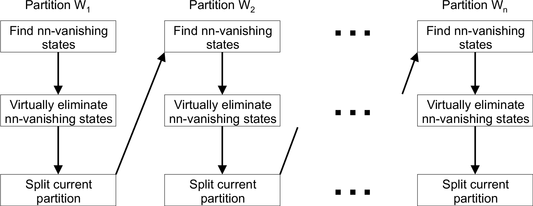
Refer to caption
Figure 2: Proposed algorithm

This paper is a major rework of our report [7]. While the algorithm is completely the same, the correctness proofs of the previous paper relied heavily on results of [1, 2]. The present paper provides a new line of argumentation and new proofs, independent of Thm. 2 of [1, 2] .

The paper is organised as follows: In Sec. 2 we present the necessary preliminaries and recall a mapping from MA to PA from [1]. Sec. 3 recapitulates some facts on weak and naïve weak bisimulation for MA. In Sec. 4 we define different notions of vanishing states and use them to relate weak bisimulation and naïve weak bisimulation. Sec. 5 discusses properties of vanishing states and provides the main theorems. Sec. 6 describes our decision algorithm for weak MA bisimulation that heavily relies on Sec. 4 and Sec. 5. In Sec. 7 we briefly discuss the applicability of our concepts and our decision algorithm to the weak bisimulation published in [6]. In Sec. 8 we compare our concepts to a recently published alternative approach [8] for deciding weak MA bisimulation. Finally, Sec. 9 concludes the paper.

2 Preliminaries

This section introduces some common notations on distributions, defines Markov Automata following [1, 2] and recalls the mapping from Markov Automata to probabilistic automata which is used in Sec. 3 to define weak bisimulation for Markov Automata.

2.1 Probability (Sub-)Distributions

First we define the notion of discrete subdistribution and related terms and notations: A mapping μ:S→[0,1]\mu:S\rightarrow[0,1] is called (discrete) subdistribution, if ∑s∈Sμ⁡(s)≤1\sum_{s\in S}\mu(s)\leq 1. As usual we write μ⁡(S′)\mu(S^{\prime}) for ∑s∈S′μ⁡(s)\sum_{s\in S^{\prime}}\mu(s). The support of μ\mu is defined as S​u​p​p​(μ):={s∈S∣μ⁡(s)>0}Supp(\mu):=\{\,s\in S\mid\mu(s)>0\,\}. The empty subdistribution μ∅\mu_{\emptyset} is defined by S​u​p​p​(μ∅)=∅Supp(\mu_{\emptyset})=\emptyset. The size of μ\mu is defined as |μ|:=μ⁡(S)|\mu|:=\mu(S). A subdistribution μ\mu is called distribution if |μ|=1|\mu|=1. The sets Dist⁡(S)\mathrm{Dist}(S) and SubDist⁡(S)\mathrm{SubDist}(S) denote distributions and subdistributions defined over the set SS. Let Δs∈Dist⁡(S)\Delta_{s}\in\mathrm{Dist}(S) denote the Dirac distribution on ss, i.e. Δs​(s)=1\Delta_{s}(s)=1. For two subdistributions μ\mu, μ′\mu^{\prime} the sum μ′′:=μ⊕μ′\mu^{\prime\prime}:=\mu\oplus\mu^{\prime} is defined as μ′′​(s):=μ⁡(s)+μ′​(s)\mu^{\prime\prime}(s):=\mu(s)+\mu^{\prime}(s) (as long as |μ′′|≤1|\mu^{\prime\prime}|\leq 1). As long as c⋅|μ|≤1c\cdot|\mu|\leq 1, we denote by c​μc\mu the subdistribution defined by (c​μ)​(s):=c⋅μ​(s)(c\mu)(s):=c\cdot\mu(s). For a subdistribution μ\mu and a state s∈S​u​p​p​(μ)s\in Supp(\mu) we define μ−s\mu-s by

(μ−s)​(t)={μ⁡(t) for ​t≠s0 for ​t=s(\mu-s)(t)=\begin{cases}\mu(t)&\text{ for }t\neq s\\ 0&\text{ for }t=s\end{cases}

Occasionally, we will also need the lifting of relations to distributions:

Definition 1 (Lifting of equivalence relations to distributions).

An equivalence relation R⊆S×SR\subseteq S\times S is lifted to D​i​s​t​(S)×D​i​s​t​(S)Dist(S)\times Dist(S) in the following way: For μ,γ∈D​i​s​t​(S)\mu,\gamma\in Dist(S) we write μ≡Rγ\mu\equiv_{R}\gamma (or simply, by abuse of notation, μ𝑅γ\mu\mathbin{R}\gamma) if and only if for each equivalence class C∈S/R:μ⁡(C)=γ⁡(C)C\in\nicefrac{{S}}{{R}}:\mu(C)=\gamma(C).

2.2 Markov and Probabilistic Automata

The definition of Markov Automata we use is the one from [1, 2].

Definition 2 (Markov Automata [1]).

A Markov automaton MA is a tuple (S,Act,            ,                 ,s0)(S,Act,\mathrel{\raisebox{1.63612pt}{\hbox to15.8pt{\vbox to3.2pt{\pgfpicture\makeatletter\hbox{\hskip 6.9pt\lower-2.7pt\hbox to0.0pt{\lxSVG@begingroup@{_scopebegin=1} \lxSVG@begingroup@{stroke=#000000} \lxSVG@begingroup@{fill=#000000} \lxSVG@setlinewidth{\the\pgflinewidth}\lxSVG@begingroup@{stroke-width=0.4pt} \lx@inpgf@ignorespaces\nullfont\hbox to0.0pt{\lxSVG@begingroup@{_scopebegin=1} {{}}\lx@inpgf@ignorespaces\hbox{\hbox{{\lxSVG@begingroup@{_scopebegin=1} {{}{}{{ {}{}}}{ {}{}} {{}{{\lx@inpgf@ignorespaces}}}{{}{\lx@inpgf@ignorespaces}}{}{{}{\lx@inpgf@ignorespaces}} {\lx@inpgf@ignorespaces }{{{{\lx@inpgf@ignorespaces}}\lxSVG@begingroup@{_scopebegin=1} \lxSVG@transformcm{1.0}{0.0}{0.0}{1.0}{0.0pt}{0.0pt}\lxSVG@begingroup@{transform=matrix(1.0 0.0 0.0 1.0 0 0)} \pgfsys@hbox{62}\lxSVG@closescope }}} \lxSVG@closescope }}} {{\lx@inpgf@ignorespaces}{}}{{\lx@inpgf@ignorespaces}}\lx@inpgf@ignorespaces\hbox{\hbox{{\lxSVG@begingroup@{_scopebegin=1} {{}{{}}{}{}} \lxSVG@closescope }}} { {}}{}{{\lx@inpgf@ignorespaces}{}}{{}}{}{}{{\lx@inpgf@ignorespaces}}\lx@inpgf@ignorespaces\hbox{\hbox{{\lxSVG@begingroup@{_scopebegin=1} {{}{{}}{}{}} \lxSVG@closescope }}} { {}}{}{{}}{}{}{{}}{}{}\lxSVG@stroke\lxSVG@drawpath@unclipped{M 3.74 -2.35}{fill:none} \lx@inpgf@ignorespaces\hbox{\hbox{{\lxSVG@begingroup@{_scopebegin=1} {\lx@inpgf@ignorespaces}{{}}{}{{}} {}{}{}{{ {{} {}{}{} {} {}{}{} \lxSVG@fill}} }{}{}{{}}\lxSVG@stroke\lxSVG@drawpath@unclipped{M 3.74 -2.35 L 7.06 -2.35}{fill:none} {{}{{}}{}{}{{}}{{{\lx@inpgf@ignorespaces}}{{{\lx@inpgf@ignorespaces}}{\lxSVG@begingroup@{_scopebegin=1} \lxSVG@transformcm{1.0}{0.0}{0.0}{1.0}{5.10005pt}{-1.7pt}\lxSVG@begingroup@{transform=matrix(1.0 0.0 0.0 1.0 7.06 -2.35)} \lxSVG@begingroup@{_scopebegin=1} \lxSVG@drawpath@unclipped{M 4.98 0 C 3.51 0.28 1.11 1.11 -0.55 2.08 L -0.55 -2.08 C 1.11 -1.11 3.51 -0.28 4.98 0}{stroke:none} \lxSVG@closescope \lxSVG@closescope }}{{\lx@inpgf@ignorespaces}}}}\lx@inpgf@ignorespaces \lxSVG@closescope }}} {{}}{}{{\lx@inpgf@ignorespaces}{}}{{}}{}{}{{}}{}{ {}}{}{{}}{} {}{}{}\lxSVG@stroke\lxSVG@drawpath@unclipped{M -9.27 -2.35 L 3.74 -2.35}{fill:none} \lx@inpgf@ignorespaces { {}}{}{{\lx@inpgf@ignorespaces}{}}{{}}{}{}{{}}{}{{{}}{\lx@inpgf@ignorespaces}{}{\lx@inpgf@ignorespaces}{}{}{}{}{}}\lxSVG@fill\lxSVG@drawpath@unclipped{M 2.35 -2.35 M 3.74 -2.35 C 3.74 -1.59 3.12 -0.97 2.35 -0.97 C 1.59 -0.97 0.97 -1.59 0.97 -2.35 C 0.97 -3.12 1.59 -3.74 2.35 -3.74 C 3.12 -3.74 3.74 -3.12 3.74 -2.35 Z M 2.35 -2.35}{stroke:none} \lx@inpgf@ignorespaces \lxSVG@closescope {\lx@inpgf@ignorespaces}{\lx@inpgf@ignorespaces}{\lx@inpgf@ignorespaces}\hss}\lxSVG@discardpath\lxSVG@closescope \hss}}\lxSVG@closescope\endpgfpicture}}}},\mathrel{\raisebox{2.36806pt}{\hbox to15.8pt{\vbox to2.4pt{\pgfpicture\makeatletter\hbox{\hskip 6.9pt\lower-1.9pt\hbox to0.0pt{\lxSVG@begingroup@{_scopebegin=1} \lxSVG@begingroup@{stroke=#000000} \lxSVG@begingroup@{fill=#000000} \lxSVG@setlinewidth{\the\pgflinewidth}\lxSVG@begingroup@{stroke-width=0.4pt} \lx@inpgf@ignorespaces\nullfont\hbox to0.0pt{\lxSVG@begingroup@{_scopebegin=1} {{}}\lx@inpgf@ignorespaces\hbox{\hbox{{\lxSVG@begingroup@{_scopebegin=1} {{}{}{{ {}{}}}{ {}{}} {{}{{\lx@inpgf@ignorespaces}}}{{}{\lx@inpgf@ignorespaces}}{}{{}{\lx@inpgf@ignorespaces}} {\lx@inpgf@ignorespaces }{{{{\lx@inpgf@ignorespaces}}\lxSVG@begingroup@{_scopebegin=1} \lxSVG@transformcm{1.0}{0.0}{0.0}{1.0}{0.0pt}{0.0pt}\lxSVG@begingroup@{transform=matrix(1.0 0.0 0.0 1.0 0 0)} \pgfsys@hbox{62}\lxSVG@closescope }}} \lxSVG@closescope }}} {{\lx@inpgf@ignorespaces}{}}{{\lx@inpgf@ignorespaces}}\lx@inpgf@ignorespaces\hbox{\hbox{{\lxSVG@begingroup@{_scopebegin=1} {{}{{}}{}{}} \lxSVG@closescope }}} { {}}{}{{\lx@inpgf@ignorespaces}{}}{{}}{}{}{{\lx@inpgf@ignorespaces}}\lx@inpgf@ignorespaces\hbox{\hbox{{\lxSVG@begingroup@{_scopebegin=1} {{}{{}}{}{}} \lxSVG@closescope }}} { {}}{}{{}}{}{}{{}}{}{}\lxSVG@stroke\lxSVG@drawpath@unclipped{M 3.74 -2.35}{fill:none} \lx@inpgf@ignorespaces\hbox{\hbox{{\lxSVG@begingroup@{_scopebegin=1} {\lx@inpgf@ignorespaces}{{}}{}{{}} {}{}{}{}{}{}{}{}{{}}\lxSVG@stroke\lxSVG@drawpath@unclipped{M 3.74 -2.35 L 7.06 -2.35}{fill:none} {{}{{}}{}{}{{}}{{{\lx@inpgf@ignorespaces}}{{{\lx@inpgf@ignorespaces}}{\lxSVG@begingroup@{_scopebegin=1} \lxSVG@transformcm{1.0}{0.0}{0.0}{1.0}{-2.89983pt}{-1.7pt}\lxSVG@begingroup@{transform=matrix(1.0 0.0 0.0 1.0 -4.01 -2.35)} \lxSVG@begingroup@{_scopebegin=1} \lxSVG@drawpath@unclipped{M 4.98 0 C 3.51 0.28 1.11 1.11 -0.55 2.08 L -0.55 -2.08 C 1.11 -1.11 3.51 -0.28 4.98 0}{stroke:none} \lxSVG@closescope \lxSVG@closescope }}{{\lx@inpgf@ignorespaces}}{{{\lx@inpgf@ignorespaces}}{\lxSVG@begingroup@{_scopebegin=1} \lxSVG@transformcm{1.0}{0.0}{0.0}{1.0}{1.10011pt}{-1.7pt}\lxSVG@begingroup@{transform=matrix(1.0 0.0 0.0 1.0 1.52 -2.35)} \lxSVG@begingroup@{_scopebegin=1} \lxSVG@drawpath@unclipped{M 4.98 0 C 3.51 0.28 1.11 1.11 -0.55 2.08 L -0.55 -2.08 C 1.11 -1.11 3.51 -0.28 4.98 0}{stroke:none} \lxSVG@closescope \lxSVG@closescope }}{{\lx@inpgf@ignorespaces}}{{{\lx@inpgf@ignorespaces}}{\lxSVG@begingroup@{_scopebegin=1} \lxSVG@transformcm{1.0}{0.0}{0.0}{1.0}{5.10005pt}{-1.7pt}\lxSVG@begingroup@{transform=matrix(1.0 0.0 0.0 1.0 7.06 -2.35)} \lxSVG@begingroup@{_scopebegin=1} \lxSVG@drawpath@unclipped{M 4.98 0 C 3.51 0.28 1.11 1.11 -0.55 2.08 L -0.55 -2.08 C 1.11 -1.11 3.51 -0.28 4.98 0}{stroke:none} \lxSVG@closescope \lxSVG@closescope }}{{\lx@inpgf@ignorespaces}}}}\lx@inpgf@ignorespaces \lxSVG@closescope }}} {{}}{}{{\lx@inpgf@ignorespaces}{}}{{}}{}{}{{}}{}{ {}}{}{{}}{} {}{}{}\lxSVG@stroke\lxSVG@drawpath@unclipped{M -9.27 -2.35 L 3.74 -2.35}{fill:none} \lx@inpgf@ignorespaces \lxSVG@closescope {\lx@inpgf@ignorespaces}{\lx@inpgf@ignorespaces}{\lx@inpgf@ignorespaces}\hss}\lxSVG@discardpath\lxSVG@closescope \hss}}\lxSVG@closescope\endpgfpicture}}}},s_{0}), where

  • •

    SS is a nonempty finite set of states,

  • •

    A​c​tAct is a set of actions containing the internal action τ\tau,

  • •

                ⊆S×Act×Dist(S)\mathrel{\raisebox{1.63612pt}{\hbox to15.8pt{\vbox to3.2pt{\pgfpicture\makeatletter\hbox{\hskip 6.9pt\lower-2.7pt\hbox to0.0pt{\lxSVG@begingroup@{_scopebegin=1} \lxSVG@begingroup@{stroke=#000000} \lxSVG@begingroup@{fill=#000000} \lxSVG@setlinewidth{\the\pgflinewidth}\lxSVG@begingroup@{stroke-width=0.4pt} \lx@inpgf@ignorespaces\nullfont\hbox to0.0pt{\lxSVG@begingroup@{_scopebegin=1} {{}}\lx@inpgf@ignorespaces\hbox{\hbox{{\lxSVG@begingroup@{_scopebegin=1} {{}{}{{ {}{}}}{ {}{}} {{}{{\lx@inpgf@ignorespaces}}}{{}{\lx@inpgf@ignorespaces}}{}{{}{\lx@inpgf@ignorespaces}} {\lx@inpgf@ignorespaces }{{{{\lx@inpgf@ignorespaces}}\lxSVG@begingroup@{_scopebegin=1} \lxSVG@transformcm{1.0}{0.0}{0.0}{1.0}{0.0pt}{0.0pt}\lxSVG@begingroup@{transform=matrix(1.0 0.0 0.0 1.0 0 0)} \pgfsys@hbox{62}\lxSVG@closescope }}} \lxSVG@closescope }}} {{\lx@inpgf@ignorespaces}{}}{{\lx@inpgf@ignorespaces}}\lx@inpgf@ignorespaces\hbox{\hbox{{\lxSVG@begingroup@{_scopebegin=1} {{}{{}}{}{}} \lxSVG@closescope }}} { {}}{}{{\lx@inpgf@ignorespaces}{}}{{}}{}{}{{\lx@inpgf@ignorespaces}}\lx@inpgf@ignorespaces\hbox{\hbox{{\lxSVG@begingroup@{_scopebegin=1} {{}{{}}{}{}} \lxSVG@closescope }}} { {}}{}{{}}{}{}{{}}{}{}\lxSVG@stroke\lxSVG@drawpath@unclipped{M 3.74 -2.35}{fill:none} \lx@inpgf@ignorespaces\hbox{\hbox{{\lxSVG@begingroup@{_scopebegin=1} {\lx@inpgf@ignorespaces}{{}}{}{{}} {}{}{}{}{}{}{{}}\lxSVG@stroke\lxSVG@drawpath@unclipped{M 3.74 -2.35 L 7.06 -2.35}{fill:none} {{}{{}}{}{}{{}}{{{\lx@inpgf@ignorespaces}}{{{\lx@inpgf@ignorespaces}}{\lxSVG@begingroup@{_scopebegin=1} \lxSVG@transformcm{1.0}{0.0}{0.0}{1.0}{5.10005pt}{-1.7pt}\lxSVG@begingroup@{transform=matrix(1.0 0.0 0.0 1.0 7.06 -2.35)} \lxSVG@begingroup@{_scopebegin=1} \lxSVG@drawpath@unclipped{M 4.98 0 C 3.51 0.28 1.11 1.11 -0.55 2.08 L -0.55 -2.08 C 1.11 -1.11 3.51 -0.28 4.98 0}{stroke:none} \lxSVG@closescope \lxSVG@closescope }}{{\lx@inpgf@ignorespaces}}}}\lx@inpgf@ignorespaces \lxSVG@closescope }}} {{}}{}{{\lx@inpgf@ignorespaces}{}}{{}}{}{}{{}}{}{ {}}{}{{}}{} {}{}{}\lxSVG@stroke\lxSVG@drawpath@unclipped{M -9.27 -2.35 L 3.74 -2.35}{fill:none} \lx@inpgf@ignorespaces { {}}{}{{\lx@inpgf@ignorespaces}{}}{{}}{}{}{{}}{}{{{}}{\lx@inpgf@ignorespaces}{}{\lx@inpgf@ignorespaces}{}{}{}{}{}}\lxSVG@fill\lxSVG@drawpath@unclipped{M 2.35 -2.35 M 3.74 -2.35 C 3.74 -1.59 3.12 -0.97 2.35 -0.97 C 1.59 -0.97 0.97 -1.59 0.97 -2.35 C 0.97 -3.12 1.59 -3.74 2.35 -3.74 C 3.12 -3.74 3.74 -3.12 3.74 -2.35 Z M 2.35 -2.35}{stroke:none} \lx@inpgf@ignorespaces \lxSVG@closescope {\lx@inpgf@ignorespaces}{\lx@inpgf@ignorespaces}{\lx@inpgf@ignorespaces}\hss}\lxSVG@discardpath\lxSVG@closescope \hss}}\lxSVG@closescope\endpgfpicture}}}}\subseteq S\times Act\times\mathrm{Dist}(S) a set of action-labelled probabilistic transitions,

  • •

                     ⊆S×ℝ≥0×S\mathrel{\raisebox{2.36806pt}{\hbox to15.8pt{\vbox to2.4pt{\pgfpicture\makeatletter\hbox{\hskip 6.9pt\lower-1.9pt\hbox to0.0pt{\lxSVG@begingroup@{_scopebegin=1} \lxSVG@begingroup@{stroke=#000000} \lxSVG@begingroup@{fill=#000000} \lxSVG@setlinewidth{\the\pgflinewidth}\lxSVG@begingroup@{stroke-width=0.4pt} \lx@inpgf@ignorespaces\nullfont\hbox to0.0pt{\lxSVG@begingroup@{_scopebegin=1} {{}}\lx@inpgf@ignorespaces\hbox{\hbox{{\lxSVG@begingroup@{_scopebegin=1} {{}{}{{ {}{}}}{ {}{}} {{}{{\lx@inpgf@ignorespaces}}}{{}{\lx@inpgf@ignorespaces}}{}{{}{\lx@inpgf@ignorespaces}} {\lx@inpgf@ignorespaces }{{{{\lx@inpgf@ignorespaces}}\lxSVG@begingroup@{_scopebegin=1} \lxSVG@transformcm{1.0}{0.0}{0.0}{1.0}{0.0pt}{0.0pt}\lxSVG@begingroup@{transform=matrix(1.0 0.0 0.0 1.0 0 0)} \pgfsys@hbox{62}\lxSVG@closescope }}} \lxSVG@closescope }}} {{\lx@inpgf@ignorespaces}{}}{{\lx@inpgf@ignorespaces}}\lx@inpgf@ignorespaces\hbox{\hbox{{\lxSVG@begingroup@{_scopebegin=1} {{}{{}}{}{}} \lxSVG@closescope }}} { {}}{}{{\lx@inpgf@ignorespaces}{}}{{}}{}{}{{\lx@inpgf@ignorespaces}}\lx@inpgf@ignorespaces\hbox{\hbox{{\lxSVG@begingroup@{_scopebegin=1} {{}{{}}{}{}} \lxSVG@closescope }}} { {}}{}{{}}{}{}{{}}{}{}\lxSVG@stroke\lxSVG@drawpath@unclipped{M 3.74 -2.35}{fill:none} \lx@inpgf@ignorespaces\hbox{\hbox{{\lxSVG@begingroup@{_scopebegin=1} {\lx@inpgf@ignorespaces}{{}}{}{{}} {}{}{}{}{}{}{}{}{{}}\lxSVG@stroke\lxSVG@drawpath@unclipped{M 3.74 -2.35 L 7.06 -2.35}{fill:none} {{}{{}}{}{}{{}}{{{\lx@inpgf@ignorespaces}}{{{\lx@inpgf@ignorespaces}}{\lxSVG@begingroup@{_scopebegin=1} \lxSVG@transformcm{1.0}{0.0}{0.0}{1.0}{-2.89983pt}{-1.7pt}\lxSVG@begingroup@{transform=matrix(1.0 0.0 0.0 1.0 -4.01 -2.35)} \lxSVG@begingroup@{_scopebegin=1} \lxSVG@drawpath@unclipped{M 4.98 0 C 3.51 0.28 1.11 1.11 -0.55 2.08 L -0.55 -2.08 C 1.11 -1.11 3.51 -0.28 4.98 0}{stroke:none} \lxSVG@closescope \lxSVG@closescope }}{{\lx@inpgf@ignorespaces}}{{{\lx@inpgf@ignorespaces}}{\lxSVG@begingroup@{_scopebegin=1} \lxSVG@transformcm{1.0}{0.0}{0.0}{1.0}{1.10011pt}{-1.7pt}\lxSVG@begingroup@{transform=matrix(1.0 0.0 0.0 1.0 1.52 -2.35)} \lxSVG@begingroup@{_scopebegin=1} \lxSVG@drawpath@unclipped{M 4.98 0 C 3.51 0.28 1.11 1.11 -0.55 2.08 L -0.55 -2.08 C 1.11 -1.11 3.51 -0.28 4.98 0}{stroke:none} \lxSVG@closescope \lxSVG@closescope }}{{\lx@inpgf@ignorespaces}}{{{\lx@inpgf@ignorespaces}}{\lxSVG@begingroup@{_scopebegin=1} \lxSVG@transformcm{1.0}{0.0}{0.0}{1.0}{5.10005pt}{-1.7pt}\lxSVG@begingroup@{transform=matrix(1.0 0.0 0.0 1.0 7.06 -2.35)} \lxSVG@begingroup@{_scopebegin=1} \lxSVG@drawpath@unclipped{M 4.98 0 C 3.51 0.28 1.11 1.11 -0.55 2.08 L -0.55 -2.08 C 1.11 -1.11 3.51 -0.28 4.98 0}{stroke:none} \lxSVG@closescope \lxSVG@closescope }}{{\lx@inpgf@ignorespaces}}}}\lx@inpgf@ignorespaces \lxSVG@closescope }}} {{}}{}{{\lx@inpgf@ignorespaces}{}}{{}}{}{}{{}}{}{ {}}{}{{}}{} {}{}{}\lxSVG@stroke\lxSVG@drawpath@unclipped{M -9.27 -2.35 L 3.74 -2.35}{fill:none} \lx@inpgf@ignorespaces \lxSVG@closescope {\lx@inpgf@ignorespaces}{\lx@inpgf@ignorespaces}{\lx@inpgf@ignorespaces}\hss}\lxSVG@discardpath\lxSVG@closescope \hss}}\lxSVG@closescope\endpgfpicture}}}}\subseteq S\times\mathbb{R}_{\geq 0}\times S a set of Markovian timed transitions and

  • •

    s0∈Ss_{0}\in S the initial state.

A state in a MA is called stable if it has no emanating τ\tau transitions, otherwise it is called unstable. A stable state ss will be denoted by s↓s\hskip-2.84544pt\downarrow.

In order to make our decision algorithm feasible we assume in the following that, in contrast to the original definition from [1, 2], all sets in Definition 2 are finite. This means that there are finitely many states, finitely many actions and finitely many transitions.

For simplicity we define probabilistic automata (PA) in terms of MA.

Definition 3.

A probabilistic automaton (PA) is a MA P=(S,A​c​t,→,∅,s0)P=(S,Act,\mathord{\rightarrow},\emptyset,s_{0}). We also write P=(S,Act,→,s0)P=(S,Act,\rightarrow,s_{0}) if the context is clear.

This definition corresponds to a simple probabilistic automaton in the sense of Segala [9].

For the mapping from MA to PA introduced in [1] we need to define the probability distribution on successor states. In contrast to [1, 2, 10], our definition of successor distribution also takes care of the case r​a​t​e​(s)=0rate(s)=0.

Definition 4 (modified11 1 The original definition from [1, 2, 10] is problematic, as for r​a​t​e​(s)=0rate(s)=0 the fraction 00\frac{0}{0} is not defined (this case is treated separately in our definition), and for infinite sets                  \mathrel{\raisebox{2.36806pt}{\hbox to15.8pt{\vbox to2.4pt{\pgfpicture\makeatletter\hbox{\hskip 6.9pt\lower-1.9pt\hbox to0.0pt{\lxSVG@begingroup@{_scopebegin=1} \lxSVG@begingroup@{stroke=#000000} \lxSVG@begingroup@{fill=#000000} \lxSVG@setlinewidth{\the\pgflinewidth}\lxSVG@begingroup@{stroke-width=0.4pt} \lx@inpgf@ignorespaces\nullfont\hbox to0.0pt{\lxSVG@begingroup@{_scopebegin=1} {{}}\lx@inpgf@ignorespaces\hbox{\hbox{{\lxSVG@begingroup@{_scopebegin=1} {{}{}{{ {}{}}}{ {}{}} {{}{{\lx@inpgf@ignorespaces}}}{{}{\lx@inpgf@ignorespaces}}{}{{}{\lx@inpgf@ignorespaces}} {\lx@inpgf@ignorespaces }{{{{\lx@inpgf@ignorespaces}}\lxSVG@begingroup@{_scopebegin=1} \lxSVG@transformcm{1.0}{0.0}{0.0}{1.0}{0.0pt}{0.0pt}\lxSVG@begingroup@{transform=matrix(1.0 0.0 0.0 1.0 0 0)} \pgfsys@hbox{62}\lxSVG@closescope }}} \lxSVG@closescope }}} {{\lx@inpgf@ignorespaces}{}}{{\lx@inpgf@ignorespaces}}\lx@inpgf@ignorespaces\hbox{\hbox{{\lxSVG@begingroup@{_scopebegin=1} {{}{{}}{}{}} \lxSVG@closescope }}} { {}}{}{{\lx@inpgf@ignorespaces}{}}{{}}{}{}{{\lx@inpgf@ignorespaces}}\lx@inpgf@ignorespaces\hbox{\hbox{{\lxSVG@begingroup@{_scopebegin=1} {{}{{}}{}{}} \lxSVG@closescope }}} { {}}{}{{}}{}{}{{}}{}{}\lxSVG@stroke\lxSVG@drawpath@unclipped{M 3.74 -2.35}{fill:none} \lx@inpgf@ignorespaces\hbox{\hbox{{\lxSVG@begingroup@{_scopebegin=1} {\lx@inpgf@ignorespaces}{{}}{}{{}} {}{}{}{}{}{}{}{}{{}}\lxSVG@stroke\lxSVG@drawpath@unclipped{M 3.74 -2.35 L 7.06 -2.35}{fill:none} {{}{{}}{}{}{{}}{{{\lx@inpgf@ignorespaces}}{{{\lx@inpgf@ignorespaces}}{\lxSVG@begingroup@{_scopebegin=1} \lxSVG@transformcm{1.0}{0.0}{0.0}{1.0}{-2.89983pt}{-1.7pt}\lxSVG@begingroup@{transform=matrix(1.0 0.0 0.0 1.0 -4.01 -2.35)} \lxSVG@begingroup@{_scopebegin=1} \lxSVG@drawpath@unclipped{M 4.98 0 C 3.51 0.28 1.11 1.11 -0.55 2.08 L -0.55 -2.08 C 1.11 -1.11 3.51 -0.28 4.98 0}{stroke:none} \lxSVG@closescope \lxSVG@closescope }}{{\lx@inpgf@ignorespaces}}{{{\lx@inpgf@ignorespaces}}{\lxSVG@begingroup@{_scopebegin=1} \lxSVG@transformcm{1.0}{0.0}{0.0}{1.0}{1.10011pt}{-1.7pt}\lxSVG@begingroup@{transform=matrix(1.0 0.0 0.0 1.0 1.52 -2.35)} \lxSVG@begingroup@{_scopebegin=1} \lxSVG@drawpath@unclipped{M 4.98 0 C 3.51 0.28 1.11 1.11 -0.55 2.08 L -0.55 -2.08 C 1.11 -1.11 3.51 -0.28 4.98 0}{stroke:none} \lxSVG@closescope \lxSVG@closescope }}{{\lx@inpgf@ignorespaces}}{{{\lx@inpgf@ignorespaces}}{\lxSVG@begingroup@{_scopebegin=1} \lxSVG@transformcm{1.0}{0.0}{0.0}{1.0}{5.10005pt}{-1.7pt}\lxSVG@begingroup@{transform=matrix(1.0 0.0 0.0 1.0 7.06 -2.35)} \lxSVG@begingroup@{_scopebegin=1} \lxSVG@drawpath@unclipped{M 4.98 0 C 3.51 0.28 1.11 1.11 -0.55 2.08 L -0.55 -2.08 C 1.11 -1.11 3.51 -0.28 4.98 0}{stroke:none} \lxSVG@closescope \lxSVG@closescope }}{{\lx@inpgf@ignorespaces}}}}\lx@inpgf@ignorespaces \lxSVG@closescope }}} {{}}{}{{\lx@inpgf@ignorespaces}{}}{{}}{}{}{{}}{}{ {}}{}{{}}{} {}{}{}\lxSVG@stroke\lxSVG@drawpath@unclipped{M -9.27 -2.35 L 3.74 -2.35}{fill:none} \lx@inpgf@ignorespaces \lxSVG@closescope {\lx@inpgf@ignorespaces}{\lx@inpgf@ignorespaces}{\lx@inpgf@ignorespaces}\hss}\lxSVG@discardpath\lxSVG@closescope \hss}}\lxSVG@closescope\endpgfpicture}}}} the exit rate may not converge (this case is not problematic for us, as we deal with finite sets). Both issues have no impact on the decision algorithm presented here, but the first issue has an impact on the compositionality of MA bisimulation in general. For a detailed explanation of why compositionality is lost with the original definitions of [1, 2, 10] we refer to Appendix A of [7]. version of Definition 3 in [1]).

Let M=(S,A​c​t,            ,                 ,s0)M=(S,Act,\mathord{\mathrel{\raisebox{1.63612pt}{\hbox to15.8pt{\vbox to3.2pt{\pgfpicture\makeatletter\hbox{\hskip 6.9pt\lower-2.7pt\hbox to0.0pt{\lxSVG@begingroup@{_scopebegin=1} \lxSVG@begingroup@{stroke=#000000} \lxSVG@begingroup@{fill=#000000} \lxSVG@setlinewidth{\the\pgflinewidth}\lxSVG@begingroup@{stroke-width=0.4pt} \lx@inpgf@ignorespaces\nullfont\hbox to0.0pt{\lxSVG@begingroup@{_scopebegin=1} {{}}\lx@inpgf@ignorespaces\hbox{\hbox{{\lxSVG@begingroup@{_scopebegin=1} {{}{}{{ {}{}}}{ {}{}} {{}{{\lx@inpgf@ignorespaces}}}{{}{\lx@inpgf@ignorespaces}}{}{{}{\lx@inpgf@ignorespaces}} {\lx@inpgf@ignorespaces }{{{{\lx@inpgf@ignorespaces}}\lxSVG@begingroup@{_scopebegin=1} \lxSVG@transformcm{1.0}{0.0}{0.0}{1.0}{0.0pt}{0.0pt}\lxSVG@begingroup@{transform=matrix(1.0 0.0 0.0 1.0 0 0)} \pgfsys@hbox{62}\lxSVG@closescope }}} \lxSVG@closescope }}} {{\lx@inpgf@ignorespaces}{}}{{\lx@inpgf@ignorespaces}}\lx@inpgf@ignorespaces\hbox{\hbox{{\lxSVG@begingroup@{_scopebegin=1} {{}{{}}{}{}} \lxSVG@closescope }}} { {}}{}{{\lx@inpgf@ignorespaces}{}}{{}}{}{}{{\lx@inpgf@ignorespaces}}\lx@inpgf@ignorespaces\hbox{\hbox{{\lxSVG@begingroup@{_scopebegin=1} {{}{{}}{}{}} \lxSVG@closescope }}} { {}}{}{{}}{}{}{{}}{}{}\lxSVG@stroke\lxSVG@drawpath@unclipped{M 3.74 -2.35}{fill:none} \lx@inpgf@ignorespaces\hbox{\hbox{{\lxSVG@begingroup@{_scopebegin=1} {\lx@inpgf@ignorespaces}{{}}{}{{}} {}{}{}{}{}{}{{}}\lxSVG@stroke\lxSVG@drawpath@unclipped{M 3.74 -2.35 L 7.06 -2.35}{fill:none} {{}{{}}{}{}{{}}{{{\lx@inpgf@ignorespaces}}{{{\lx@inpgf@ignorespaces}}{\lxSVG@begingroup@{_scopebegin=1} \lxSVG@transformcm{1.0}{0.0}{0.0}{1.0}{5.10005pt}{-1.7pt}\lxSVG@begingroup@{transform=matrix(1.0 0.0 0.0 1.0 7.06 -2.35)} \lxSVG@begingroup@{_scopebegin=1} \lxSVG@drawpath@unclipped{M 4.98 0 C 3.51 0.28 1.11 1.11 -0.55 2.08 L -0.55 -2.08 C 1.11 -1.11 3.51 -0.28 4.98 0}{stroke:none} \lxSVG@closescope \lxSVG@closescope }}{{\lx@inpgf@ignorespaces}}}}\lx@inpgf@ignorespaces \lxSVG@closescope }}} {{}}{}{{\lx@inpgf@ignorespaces}{}}{{}}{}{}{{}}{}{ {}}{}{{}}{} {}{}{}\lxSVG@stroke\lxSVG@drawpath@unclipped{M -9.27 -2.35 L 3.74 -2.35}{fill:none} \lx@inpgf@ignorespaces { {}}{}{{\lx@inpgf@ignorespaces}{}}{{}}{}{}{{}}{}{{{}}{\lx@inpgf@ignorespaces}{}{\lx@inpgf@ignorespaces}{}{}{}{}{}}\lxSVG@fill\lxSVG@drawpath@unclipped{M 2.35 -2.35 M 3.74 -2.35 C 3.74 -1.59 3.12 -0.97 2.35 -0.97 C 1.59 -0.97 0.97 -1.59 0.97 -2.35 C 0.97 -3.12 1.59 -3.74 2.35 -3.74 C 3.12 -3.74 3.74 -3.12 3.74 -2.35 Z M 2.35 -2.35}{stroke:none} \lx@inpgf@ignorespaces \lxSVG@closescope {\lx@inpgf@ignorespaces}{\lx@inpgf@ignorespaces}{\lx@inpgf@ignorespaces}\hss}\lxSVG@discardpath\lxSVG@closescope \hss}}\lxSVG@closescope\endpgfpicture}}}}},\mathord{\mathrel{\raisebox{2.36806pt}{\hbox to15.8pt{\vbox to2.4pt{\pgfpicture\makeatletter\hbox{\hskip 6.9pt\lower-1.9pt\hbox to0.0pt{\lxSVG@begingroup@{_scopebegin=1} \lxSVG@begingroup@{stroke=#000000} \lxSVG@begingroup@{fill=#000000} \lxSVG@setlinewidth{\the\pgflinewidth}\lxSVG@begingroup@{stroke-width=0.4pt} \lx@inpgf@ignorespaces\nullfont\hbox to0.0pt{\lxSVG@begingroup@{_scopebegin=1} {{}}\lx@inpgf@ignorespaces\hbox{\hbox{{\lxSVG@begingroup@{_scopebegin=1} {{}{}{{ {}{}}}{ {}{}} {{}{{\lx@inpgf@ignorespaces}}}{{}{\lx@inpgf@ignorespaces}}{}{{}{\lx@inpgf@ignorespaces}} {\lx@inpgf@ignorespaces }{{{{\lx@inpgf@ignorespaces}}\lxSVG@begingroup@{_scopebegin=1} \lxSVG@transformcm{1.0}{0.0}{0.0}{1.0}{0.0pt}{0.0pt}\lxSVG@begingroup@{transform=matrix(1.0 0.0 0.0 1.0 0 0)} \pgfsys@hbox{62}\lxSVG@closescope }}} \lxSVG@closescope }}} {{\lx@inpgf@ignorespaces}{}}{{\lx@inpgf@ignorespaces}}\lx@inpgf@ignorespaces\hbox{\hbox{{\lxSVG@begingroup@{_scopebegin=1} {{}{{}}{}{}} \lxSVG@closescope }}} { {}}{}{{\lx@inpgf@ignorespaces}{}}{{}}{}{}{{\lx@inpgf@ignorespaces}}\lx@inpgf@ignorespaces\hbox{\hbox{{\lxSVG@begingroup@{_scopebegin=1} {{}{{}}{}{}} \lxSVG@closescope }}} { {}}{}{{}}{}{}{{}}{}{}\lxSVG@stroke\lxSVG@drawpath@unclipped{M 3.74 -2.35}{fill:none} \lx@inpgf@ignorespaces\hbox{\hbox{{\lxSVG@begingroup@{_scopebegin=1} {\lx@inpgf@ignorespaces}{{}}{}{{}} {}{}{}{}{}{}{}{}{{}}\lxSVG@stroke\lxSVG@drawpath@unclipped{M 3.74 -2.35 L 7.06 -2.35}{fill:none} {{}{{}}{}{}{{}}{{{\lx@inpgf@ignorespaces}}{{{\lx@inpgf@ignorespaces}}{\lxSVG@begingroup@{_scopebegin=1} \lxSVG@transformcm{1.0}{0.0}{0.0}{1.0}{-2.89983pt}{-1.7pt}\lxSVG@begingroup@{transform=matrix(1.0 0.0 0.0 1.0 -4.01 -2.35)} \lxSVG@begingroup@{_scopebegin=1} \lxSVG@drawpath@unclipped{M 4.98 0 C 3.51 0.28 1.11 1.11 -0.55 2.08 L -0.55 -2.08 C 1.11 -1.11 3.51 -0.28 4.98 0}{stroke:none} \lxSVG@closescope \lxSVG@closescope }}{{\lx@inpgf@ignorespaces}}{{{\lx@inpgf@ignorespaces}}{\lxSVG@begingroup@{_scopebegin=1} \lxSVG@transformcm{1.0}{0.0}{0.0}{1.0}{1.10011pt}{-1.7pt}\lxSVG@begingroup@{transform=matrix(1.0 0.0 0.0 1.0 1.52 -2.35)} \lxSVG@begingroup@{_scopebegin=1} \lxSVG@drawpath@unclipped{M 4.98 0 C 3.51 0.28 1.11 1.11 -0.55 2.08 L -0.55 -2.08 C 1.11 -1.11 3.51 -0.28 4.98 0}{stroke:none} \lxSVG@closescope \lxSVG@closescope }}{{\lx@inpgf@ignorespaces}}{{{\lx@inpgf@ignorespaces}}{\lxSVG@begingroup@{_scopebegin=1} \lxSVG@transformcm{1.0}{0.0}{0.0}{1.0}{5.10005pt}{-1.7pt}\lxSVG@begingroup@{transform=matrix(1.0 0.0 0.0 1.0 7.06 -2.35)} \lxSVG@begingroup@{_scopebegin=1} \lxSVG@drawpath@unclipped{M 4.98 0 C 3.51 0.28 1.11 1.11 -0.55 2.08 L -0.55 -2.08 C 1.11 -1.11 3.51 -0.28 4.98 0}{stroke:none} \lxSVG@closescope \lxSVG@closescope }}{{\lx@inpgf@ignorespaces}}}}\lx@inpgf@ignorespaces \lxSVG@closescope }}} {{}}{}{{\lx@inpgf@ignorespaces}{}}{{}}{}{}{{}}{}{ {}}{}{{}}{} {}{}{}\lxSVG@stroke\lxSVG@drawpath@unclipped{M -9.27 -2.35 L 3.74 -2.35}{fill:none} \lx@inpgf@ignorespaces \lxSVG@closescope {\lx@inpgf@ignorespaces}{\lx@inpgf@ignorespaces}{\lx@inpgf@ignorespaces}\hss}\lxSVG@discardpath\lxSVG@closescope \hss}}\lxSVG@closescope\endpgfpicture}}}}},s_{0}) be a MA. Define

r​a​t​e​(s,s′):=∑(s,λ,s′)∈                 λrate(s,s^{\prime}):=\sum_{(s,\lambda,s^{\prime})\in\mathrel{\raisebox{1.65764pt}{\hbox to15.8pt{\vbox to2.4pt{\pgfpicture\makeatletter\hbox{\hskip 6.9pt\lower-1.9pt\hbox to0.0pt{\lxSVG@begingroup@{_scopebegin=1} \lxSVG@begingroup@{stroke=#000000} \lxSVG@begingroup@{fill=#000000} \lxSVG@setlinewidth{\the\pgflinewidth}\lxSVG@begingroup@{stroke-width=0.4pt} \lx@inpgf@ignorespaces\nullfont\hbox to0.0pt{\lxSVG@begingroup@{_scopebegin=1} {{}}\lx@inpgf@ignorespaces\hbox{\hbox{{\lxSVG@begingroup@{_scopebegin=1} {{}{}{{ {}{}}}{ {}{}} {{}{{\lx@inpgf@ignorespaces}}}{{}{\lx@inpgf@ignorespaces}}{}{{}{\lx@inpgf@ignorespaces}} {\lx@inpgf@ignorespaces }{{{{\lx@inpgf@ignorespaces}}\lxSVG@begingroup@{_scopebegin=1} \lxSVG@transformcm{1.0}{0.0}{0.0}{1.0}{0.0pt}{0.0pt}\lxSVG@begingroup@{transform=matrix(1.0 0.0 0.0 1.0 0 0)} \pgfsys@hbox{62}\lxSVG@closescope }}} \lxSVG@closescope }}} {{\lx@inpgf@ignorespaces}{}}{{\lx@inpgf@ignorespaces}}\lx@inpgf@ignorespaces\hbox{\hbox{{\lxSVG@begingroup@{_scopebegin=1} {{}{{}}{}{}} \lxSVG@closescope }}} { {}}{}{{\lx@inpgf@ignorespaces}{}}{{}}{}{}{{\lx@inpgf@ignorespaces}}\lx@inpgf@ignorespaces\hbox{\hbox{{\lxSVG@begingroup@{_scopebegin=1} {{}{{}}{}{}} \lxSVG@closescope }}} { {}}{}{{}}{}{}{{}}{}{}\lxSVG@stroke\lxSVG@drawpath@unclipped{M 3.74 -2.35}{fill:none} \lx@inpgf@ignorespaces\hbox{\hbox{{\lxSVG@begingroup@{_scopebegin=1} {\lx@inpgf@ignorespaces}{{}}{}{{}} {}{}{}{}{}{}{}{}{{}}\lxSVG@stroke\lxSVG@drawpath@unclipped{M 3.74 -2.35 L 7.06 -2.35}{fill:none} {{}{{}}{}{}{{}}{{{\lx@inpgf@ignorespaces}}{{{\lx@inpgf@ignorespaces}}{\lxSVG@begingroup@{_scopebegin=1} \lxSVG@transformcm{1.0}{0.0}{0.0}{1.0}{-2.89983pt}{-1.7pt}\lxSVG@begingroup@{transform=matrix(1.0 0.0 0.0 1.0 -4.01 -2.35)} \lxSVG@begingroup@{_scopebegin=1} \lxSVG@drawpath@unclipped{M 4.98 0 C 3.51 0.28 1.11 1.11 -0.55 2.08 L -0.55 -2.08 C 1.11 -1.11 3.51 -0.28 4.98 0}{stroke:none} \lxSVG@closescope \lxSVG@closescope }}{{\lx@inpgf@ignorespaces}}{{{\lx@inpgf@ignorespaces}}{\lxSVG@begingroup@{_scopebegin=1} \lxSVG@transformcm{1.0}{0.0}{0.0}{1.0}{1.10011pt}{-1.7pt}\lxSVG@begingroup@{transform=matrix(1.0 0.0 0.0 1.0 1.52 -2.35)} \lxSVG@begingroup@{_scopebegin=1} \lxSVG@drawpath@unclipped{M 4.98 0 C 3.51 0.28 1.11 1.11 -0.55 2.08 L -0.55 -2.08 C 1.11 -1.11 3.51 -0.28 4.98 0}{stroke:none} \lxSVG@closescope \lxSVG@closescope }}{{\lx@inpgf@ignorespaces}}{{{\lx@inpgf@ignorespaces}}{\lxSVG@begingroup@{_scopebegin=1} \lxSVG@transformcm{1.0}{0.0}{0.0}{1.0}{5.10005pt}{-1.7pt}\lxSVG@begingroup@{transform=matrix(1.0 0.0 0.0 1.0 7.06 -2.35)} \lxSVG@begingroup@{_scopebegin=1} \lxSVG@drawpath@unclipped{M 4.98 0 C 3.51 0.28 1.11 1.11 -0.55 2.08 L -0.55 -2.08 C 1.11 -1.11 3.51 -0.28 4.98 0}{stroke:none} \lxSVG@closescope \lxSVG@closescope }}{{\lx@inpgf@ignorespaces}}}}\lx@inpgf@ignorespaces \lxSVG@closescope }}} {{}}{}{{\lx@inpgf@ignorespaces}{}}{{}}{}{}{{}}{}{ {}}{}{{}}{} {}{}{}\lxSVG@stroke\lxSVG@drawpath@unclipped{M -9.27 -2.35 L 3.74 -2.35}{fill:none} \lx@inpgf@ignorespaces \lxSVG@closescope {\lx@inpgf@ignorespaces}{\lx@inpgf@ignorespaces}{\lx@inpgf@ignorespaces}\hss}\lxSVG@discardpath\lxSVG@closescope \hss}}\lxSVG@closescope\endpgfpicture}}}}}\lambda

and r​a​t​e​(s):=∑s′∈Sr​a​t​e​(s,s′)rate(s):=\sum_{s^{\prime}\in S}rate(s,s^{\prime}) which is called the exit rate of state ss. The probability distributions PsP_{s} are defined in the following way:

Ps:={s′↦r​a​t​e​(s,s′)r​a​t​e​(s) for ​r​a​t​e​(s)≠0Δs otherwiseP_{s}:=\begin{cases}s^{\prime}\mapsto\frac{rate(s,s^{\prime})}{rate(s)}&\text{ for }rate(s)\neq 0\\ \Delta_{s}&\text{ otherwise}\end{cases}

2.3 A mapping from MA to PA

The remarkable idea of [1] is to define bisimulations on MA using a mapping from MA to PA. The basic ingredient is a set of special actions, denoted by χ(.)\chi(.), that cover timed behaviour. In the setting of [1, 2] countable action sets are mapped to uncountable action sets by definition, as for every real number a new action name is introduced. In order to keep the action set finite to retain algorithmic tractability, we redefine A​c​tχAct^{\chi} in the context of a fixed MA:

Definition 5.

Let M=(S,Act,            ,                 ,s0)M=(S,Act,\mathrel{\raisebox{1.63612pt}{\hbox to15.8pt{\vbox to3.2pt{\pgfpicture\makeatletter\hbox{\hskip 6.9pt\lower-2.7pt\hbox to0.0pt{\lxSVG@begingroup@{_scopebegin=1} \lxSVG@begingroup@{stroke=#000000} \lxSVG@begingroup@{fill=#000000} \lxSVG@setlinewidth{\the\pgflinewidth}\lxSVG@begingroup@{stroke-width=0.4pt} \lx@inpgf@ignorespaces\nullfont\hbox to0.0pt{\lxSVG@begingroup@{_scopebegin=1} {{}}\lx@inpgf@ignorespaces\hbox{\hbox{{\lxSVG@begingroup@{_scopebegin=1} {{}{}{{ {}{}}}{ {}{}} {{}{{\lx@inpgf@ignorespaces}}}{{}{\lx@inpgf@ignorespaces}}{}{{}{\lx@inpgf@ignorespaces}} {\lx@inpgf@ignorespaces }{{{{\lx@inpgf@ignorespaces}}\lxSVG@begingroup@{_scopebegin=1} \lxSVG@transformcm{1.0}{0.0}{0.0}{1.0}{0.0pt}{0.0pt}\lxSVG@begingroup@{transform=matrix(1.0 0.0 0.0 1.0 0 0)} \pgfsys@hbox{62}\lxSVG@closescope }}} \lxSVG@closescope }}} {{\lx@inpgf@ignorespaces}{}}{{\lx@inpgf@ignorespaces}}\lx@inpgf@ignorespaces\hbox{\hbox{{\lxSVG@begingroup@{_scopebegin=1} {{}{{}}{}{}} \lxSVG@closescope }}} { {}}{}{{\lx@inpgf@ignorespaces}{}}{{}}{}{}{{\lx@inpgf@ignorespaces}}\lx@inpgf@ignorespaces\hbox{\hbox{{\lxSVG@begingroup@{_scopebegin=1} {{}{{}}{}{}} \lxSVG@closescope }}} { {}}{}{{}}{}{}{{}}{}{}\lxSVG@stroke\lxSVG@drawpath@unclipped{M 3.74 -2.35}{fill:none} \lx@inpgf@ignorespaces\hbox{\hbox{{\lxSVG@begingroup@{_scopebegin=1} {\lx@inpgf@ignorespaces}{{}}{}{{}} {}{}{}{}{}{}{{}}\lxSVG@stroke\lxSVG@drawpath@unclipped{M 3.74 -2.35 L 7.06 -2.35}{fill:none} {{}{{}}{}{}{{}}{{{\lx@inpgf@ignorespaces}}{{{\lx@inpgf@ignorespaces}}{\lxSVG@begingroup@{_scopebegin=1} \lxSVG@transformcm{1.0}{0.0}{0.0}{1.0}{5.10005pt}{-1.7pt}\lxSVG@begingroup@{transform=matrix(1.0 0.0 0.0 1.0 7.06 -2.35)} \lxSVG@begingroup@{_scopebegin=1} \lxSVG@drawpath@unclipped{M 4.98 0 C 3.51 0.28 1.11 1.11 -0.55 2.08 L -0.55 -2.08 C 1.11 -1.11 3.51 -0.28 4.98 0}{stroke:none} \lxSVG@closescope \lxSVG@closescope }}{{\lx@inpgf@ignorespaces}}}}\lx@inpgf@ignorespaces \lxSVG@closescope }}} {{}}{}{{\lx@inpgf@ignorespaces}{}}{{}}{}{}{{}}{}{ {}}{}{{}}{} {}{}{}\lxSVG@stroke\lxSVG@drawpath@unclipped{M -9.27 -2.35 L 3.74 -2.35}{fill:none} \lx@inpgf@ignorespaces { {}}{}{{\lx@inpgf@ignorespaces}{}}{{}}{}{}{{}}{}{{{}}{\lx@inpgf@ignorespaces}{}{\lx@inpgf@ignorespaces}{}{}{}{}{}}\lxSVG@fill\lxSVG@drawpath@unclipped{M 2.35 -2.35 M 3.74 -2.35 C 3.74 -1.59 3.12 -0.97 2.35 -0.97 C 1.59 -0.97 0.97 -1.59 0.97 -2.35 C 0.97 -3.12 1.59 -3.74 2.35 -3.74 C 3.12 -3.74 3.74 -3.12 3.74 -2.35 Z M 2.35 -2.35}{stroke:none} \lx@inpgf@ignorespaces \lxSVG@closescope {\lx@inpgf@ignorespaces}{\lx@inpgf@ignorespaces}{\lx@inpgf@ignorespaces}\hss}\lxSVG@discardpath\lxSVG@closescope \hss}}\lxSVG@closescope\endpgfpicture}}}},\mathrel{\raisebox{2.36806pt}{\hbox to15.8pt{\vbox to2.4pt{\pgfpicture\makeatletter\hbox{\hskip 6.9pt\lower-1.9pt\hbox to0.0pt{\lxSVG@begingroup@{_scopebegin=1} \lxSVG@begingroup@{stroke=#000000} \lxSVG@begingroup@{fill=#000000} \lxSVG@setlinewidth{\the\pgflinewidth}\lxSVG@begingroup@{stroke-width=0.4pt} \lx@inpgf@ignorespaces\nullfont\hbox to0.0pt{\lxSVG@begingroup@{_scopebegin=1} {{}}\lx@inpgf@ignorespaces\hbox{\hbox{{\lxSVG@begingroup@{_scopebegin=1} {{}{}{{ {}{}}}{ {}{}} {{}{{\lx@inpgf@ignorespaces}}}{{}{\lx@inpgf@ignorespaces}}{}{{}{\lx@inpgf@ignorespaces}} {\lx@inpgf@ignorespaces }{{{{\lx@inpgf@ignorespaces}}\lxSVG@begingroup@{_scopebegin=1} \lxSVG@transformcm{1.0}{0.0}{0.0}{1.0}{0.0pt}{0.0pt}\lxSVG@begingroup@{transform=matrix(1.0 0.0 0.0 1.0 0 0)} \pgfsys@hbox{62}\lxSVG@closescope }}} \lxSVG@closescope }}} {{\lx@inpgf@ignorespaces}{}}{{\lx@inpgf@ignorespaces}}\lx@inpgf@ignorespaces\hbox{\hbox{{\lxSVG@begingroup@{_scopebegin=1} {{}{{}}{}{}} \lxSVG@closescope }}} { {}}{}{{\lx@inpgf@ignorespaces}{}}{{}}{}{}{{\lx@inpgf@ignorespaces}}\lx@inpgf@ignorespaces\hbox{\hbox{{\lxSVG@begingroup@{_scopebegin=1} {{}{{}}{}{}} \lxSVG@closescope }}} { {}}{}{{}}{}{}{{}}{}{}\lxSVG@stroke\lxSVG@drawpath@unclipped{M 3.74 -2.35}{fill:none} \lx@inpgf@ignorespaces\hbox{\hbox{{\lxSVG@begingroup@{_scopebegin=1} {\lx@inpgf@ignorespaces}{{}}{}{{}} {}{}{}{}{}{}{}{}{{}}\lxSVG@stroke\lxSVG@drawpath@unclipped{M 3.74 -2.35 L 7.06 -2.35}{fill:none} {{}{{}}{}{}{{}}{{{\lx@inpgf@ignorespaces}}{{{\lx@inpgf@ignorespaces}}{\lxSVG@begingroup@{_scopebegin=1} \lxSVG@transformcm{1.0}{0.0}{0.0}{1.0}{-2.89983pt}{-1.7pt}\lxSVG@begingroup@{transform=matrix(1.0 0.0 0.0 1.0 -4.01 -2.35)} \lxSVG@begingroup@{_scopebegin=1} \lxSVG@drawpath@unclipped{M 4.98 0 C 3.51 0.28 1.11 1.11 -0.55 2.08 L -0.55 -2.08 C 1.11 -1.11 3.51 -0.28 4.98 0}{stroke:none} \lxSVG@closescope \lxSVG@closescope }}{{\lx@inpgf@ignorespaces}}{{{\lx@inpgf@ignorespaces}}{\lxSVG@begingroup@{_scopebegin=1} \lxSVG@transformcm{1.0}{0.0}{0.0}{1.0}{1.10011pt}{-1.7pt}\lxSVG@begingroup@{transform=matrix(1.0 0.0 0.0 1.0 1.52 -2.35)} \lxSVG@begingroup@{_scopebegin=1} \lxSVG@drawpath@unclipped{M 4.98 0 C 3.51 0.28 1.11 1.11 -0.55 2.08 L -0.55 -2.08 C 1.11 -1.11 3.51 -0.28 4.98 0}{stroke:none} \lxSVG@closescope \lxSVG@closescope }}{{\lx@inpgf@ignorespaces}}{{{\lx@inpgf@ignorespaces}}{\lxSVG@begingroup@{_scopebegin=1} \lxSVG@transformcm{1.0}{0.0}{0.0}{1.0}{5.10005pt}{-1.7pt}\lxSVG@begingroup@{transform=matrix(1.0 0.0 0.0 1.0 7.06 -2.35)} \lxSVG@begingroup@{_scopebegin=1} \lxSVG@drawpath@unclipped{M 4.98 0 C 3.51 0.28 1.11 1.11 -0.55 2.08 L -0.55 -2.08 C 1.11 -1.11 3.51 -0.28 4.98 0}{stroke:none} \lxSVG@closescope \lxSVG@closescope }}{{\lx@inpgf@ignorespaces}}}}\lx@inpgf@ignorespaces \lxSVG@closescope }}} {{}}{}{{\lx@inpgf@ignorespaces}{}}{{}}{}{}{{}}{}{ {}}{}{{}}{} {}{}{}\lxSVG@stroke\lxSVG@drawpath@unclipped{M -9.27 -2.35 L 3.74 -2.35}{fill:none} \lx@inpgf@ignorespaces \lxSVG@closescope {\lx@inpgf@ignorespaces}{\lx@inpgf@ignorespaces}{\lx@inpgf@ignorespaces}\hss}\lxSVG@discardpath\lxSVG@closescope \hss}}\lxSVG@closescope\endpgfpicture}}}},s_{0}) be a MA. Assume ∀r∈ℝ≥0 χ(r)∉Act\forall r\in\mathbb{R}_{\geq 0}\text{ }\chi(r)\notin Act and define ℛ​𝒯:={r​a​t​e​(s)|s∈S}\mathcal{RT}:=\{rate(s)|s\in S\} (which is finite). Then we define A​c​tχ⁡(ℛ​𝒯)={χ⁡(r)|r∈ℛ​𝒯}Act^{\chi(\mathcal{RT})}=\{\chi(r)|r\in\mathcal{RT}\} and A​c​tχ:=A​c​t∪A​c​tχ⁡(ℛ​𝒯)Act^{\chi}:=Act\cup Act^{\chi(\mathcal{RT})}.

There is a mapping from MA to PA (adapted from [1]) where we use Definition 4:

Definition 6.

Let M=(S,Act,            ,                 ,s0)M=(S,Act,\mathrel{\raisebox{1.63612pt}{\hbox to15.8pt{\vbox to3.2pt{\pgfpicture\makeatletter\hbox{\hskip 6.9pt\lower-2.7pt\hbox to0.0pt{\lxSVG@begingroup@{_scopebegin=1} \lxSVG@begingroup@{stroke=#000000} \lxSVG@begingroup@{fill=#000000} \lxSVG@setlinewidth{\the\pgflinewidth}\lxSVG@begingroup@{stroke-width=0.4pt} \lx@inpgf@ignorespaces\nullfont\hbox to0.0pt{\lxSVG@begingroup@{_scopebegin=1} {{}}\lx@inpgf@ignorespaces\hbox{\hbox{{\lxSVG@begingroup@{_scopebegin=1} {{}{}{{ {}{}}}{ {}{}} {{}{{\lx@inpgf@ignorespaces}}}{{}{\lx@inpgf@ignorespaces}}{}{{}{\lx@inpgf@ignorespaces}} {\lx@inpgf@ignorespaces }{{{{\lx@inpgf@ignorespaces}}\lxSVG@begingroup@{_scopebegin=1} \lxSVG@transformcm{1.0}{0.0}{0.0}{1.0}{0.0pt}{0.0pt}\lxSVG@begingroup@{transform=matrix(1.0 0.0 0.0 1.0 0 0)} \pgfsys@hbox{62}\lxSVG@closescope }}} \lxSVG@closescope }}} {{\lx@inpgf@ignorespaces}{}}{{\lx@inpgf@ignorespaces}}\lx@inpgf@ignorespaces\hbox{\hbox{{\lxSVG@begingroup@{_scopebegin=1} {{}{{}}{}{}} \lxSVG@closescope }}} { {}}{}{{\lx@inpgf@ignorespaces}{}}{{}}{}{}{{\lx@inpgf@ignorespaces}}\lx@inpgf@ignorespaces\hbox{\hbox{{\lxSVG@begingroup@{_scopebegin=1} {{}{{}}{}{}} \lxSVG@closescope }}} { {}}{}{{}}{}{}{{}}{}{}\lxSVG@stroke\lxSVG@drawpath@unclipped{M 3.74 -2.35}{fill:none} \lx@inpgf@ignorespaces\hbox{\hbox{{\lxSVG@begingroup@{_scopebegin=1} {\lx@inpgf@ignorespaces}{{}}{}{{}} {}{}{}{}{}{}{{}}\lxSVG@stroke\lxSVG@drawpath@unclipped{M 3.74 -2.35 L 7.06 -2.35}{fill:none} {{}{{}}{}{}{{}}{{{\lx@inpgf@ignorespaces}}{{{\lx@inpgf@ignorespaces}}{\lxSVG@begingroup@{_scopebegin=1} \lxSVG@transformcm{1.0}{0.0}{0.0}{1.0}{5.10005pt}{-1.7pt}\lxSVG@begingroup@{transform=matrix(1.0 0.0 0.0 1.0 7.06 -2.35)} \lxSVG@begingroup@{_scopebegin=1} \lxSVG@drawpath@unclipped{M 4.98 0 C 3.51 0.28 1.11 1.11 -0.55 2.08 L -0.55 -2.08 C 1.11 -1.11 3.51 -0.28 4.98 0}{stroke:none} \lxSVG@closescope \lxSVG@closescope }}{{\lx@inpgf@ignorespaces}}}}\lx@inpgf@ignorespaces \lxSVG@closescope }}} {{}}{}{{\lx@inpgf@ignorespaces}{}}{{}}{}{}{{}}{}{ {}}{}{{}}{} {}{}{}\lxSVG@stroke\lxSVG@drawpath@unclipped{M -9.27 -2.35 L 3.74 -2.35}{fill:none} \lx@inpgf@ignorespaces { {}}{}{{\lx@inpgf@ignorespaces}{}}{{}}{}{}{{}}{}{{{}}{\lx@inpgf@ignorespaces}{}{\lx@inpgf@ignorespaces}{}{}{}{}{}}\lxSVG@fill\lxSVG@drawpath@unclipped{M 2.35 -2.35 M 3.74 -2.35 C 3.74 -1.59 3.12 -0.97 2.35 -0.97 C 1.59 -0.97 0.97 -1.59 0.97 -2.35 C 0.97 -3.12 1.59 -3.74 2.35 -3.74 C 3.12 -3.74 3.74 -3.12 3.74 -2.35 Z M 2.35 -2.35}{stroke:none} \lx@inpgf@ignorespaces \lxSVG@closescope {\lx@inpgf@ignorespaces}{\lx@inpgf@ignorespaces}{\lx@inpgf@ignorespaces}\hss}\lxSVG@discardpath\lxSVG@closescope \hss}}\lxSVG@closescope\endpgfpicture}}}},\mathrel{\raisebox{2.36806pt}{\hbox to15.8pt{\vbox to2.4pt{\pgfpicture\makeatletter\hbox{\hskip 6.9pt\lower-1.9pt\hbox to0.0pt{\lxSVG@begingroup@{_scopebegin=1} \lxSVG@begingroup@{stroke=#000000} \lxSVG@begingroup@{fill=#000000} \lxSVG@setlinewidth{\the\pgflinewidth}\lxSVG@begingroup@{stroke-width=0.4pt} \lx@inpgf@ignorespaces\nullfont\hbox to0.0pt{\lxSVG@begingroup@{_scopebegin=1} {{}}\lx@inpgf@ignorespaces\hbox{\hbox{{\lxSVG@begingroup@{_scopebegin=1} {{}{}{{ {}{}}}{ {}{}} {{}{{\lx@inpgf@ignorespaces}}}{{}{\lx@inpgf@ignorespaces}}{}{{}{\lx@inpgf@ignorespaces}} {\lx@inpgf@ignorespaces }{{{{\lx@inpgf@ignorespaces}}\lxSVG@begingroup@{_scopebegin=1} \lxSVG@transformcm{1.0}{0.0}{0.0}{1.0}{0.0pt}{0.0pt}\lxSVG@begingroup@{transform=matrix(1.0 0.0 0.0 1.0 0 0)} \pgfsys@hbox{62}\lxSVG@closescope }}} \lxSVG@closescope }}} {{\lx@inpgf@ignorespaces}{}}{{\lx@inpgf@ignorespaces}}\lx@inpgf@ignorespaces\hbox{\hbox{{\lxSVG@begingroup@{_scopebegin=1} {{}{{}}{}{}} \lxSVG@closescope }}} { {}}{}{{\lx@inpgf@ignorespaces}{}}{{}}{}{}{{\lx@inpgf@ignorespaces}}\lx@inpgf@ignorespaces\hbox{\hbox{{\lxSVG@begingroup@{_scopebegin=1} {{}{{}}{}{}} \lxSVG@closescope }}} { {}}{}{{}}{}{}{{}}{}{}\lxSVG@stroke\lxSVG@drawpath@unclipped{M 3.74 -2.35}{fill:none} \lx@inpgf@ignorespaces\hbox{\hbox{{\lxSVG@begingroup@{_scopebegin=1} {\lx@inpgf@ignorespaces}{{}}{}{{}} {}{}{}{}{}{}{}{}{{}}\lxSVG@stroke\lxSVG@drawpath@unclipped{M 3.74 -2.35 L 7.06 -2.35}{fill:none} {{}{{}}{}{}{{}}{{{\lx@inpgf@ignorespaces}}{{{\lx@inpgf@ignorespaces}}{\lxSVG@begingroup@{_scopebegin=1} \lxSVG@transformcm{1.0}{0.0}{0.0}{1.0}{-2.89983pt}{-1.7pt}\lxSVG@begingroup@{transform=matrix(1.0 0.0 0.0 1.0 -4.01 -2.35)} \lxSVG@begingroup@{_scopebegin=1} \lxSVG@drawpath@unclipped{M 4.98 0 C 3.51 0.28 1.11 1.11 -0.55 2.08 L -0.55 -2.08 C 1.11 -1.11 3.51 -0.28 4.98 0}{stroke:none} \lxSVG@closescope \lxSVG@closescope }}{{\lx@inpgf@ignorespaces}}{{{\lx@inpgf@ignorespaces}}{\lxSVG@begingroup@{_scopebegin=1} \lxSVG@transformcm{1.0}{0.0}{0.0}{1.0}{1.10011pt}{-1.7pt}\lxSVG@begingroup@{transform=matrix(1.0 0.0 0.0 1.0 1.52 -2.35)} \lxSVG@begingroup@{_scopebegin=1} \lxSVG@drawpath@unclipped{M 4.98 0 C 3.51 0.28 1.11 1.11 -0.55 2.08 L -0.55 -2.08 C 1.11 -1.11 3.51 -0.28 4.98 0}{stroke:none} \lxSVG@closescope \lxSVG@closescope }}{{\lx@inpgf@ignorespaces}}{{{\lx@inpgf@ignorespaces}}{\lxSVG@begingroup@{_scopebegin=1} \lxSVG@transformcm{1.0}{0.0}{0.0}{1.0}{5.10005pt}{-1.7pt}\lxSVG@begingroup@{transform=matrix(1.0 0.0 0.0 1.0 7.06 -2.35)} \lxSVG@begingroup@{_scopebegin=1} \lxSVG@drawpath@unclipped{M 4.98 0 C 3.51 0.28 1.11 1.11 -0.55 2.08 L -0.55 -2.08 C 1.11 -1.11 3.51 -0.28 4.98 0}{stroke:none} \lxSVG@closescope \lxSVG@closescope }}{{\lx@inpgf@ignorespaces}}}}\lx@inpgf@ignorespaces \lxSVG@closescope }}} {{}}{}{{\lx@inpgf@ignorespaces}{}}{{}}{}{}{{}}{}{ {}}{}{{}}{} {}{}{}\lxSVG@stroke\lxSVG@drawpath@unclipped{M -9.27 -2.35 L 3.74 -2.35}{fill:none} \lx@inpgf@ignorespaces \lxSVG@closescope {\lx@inpgf@ignorespaces}{\lx@inpgf@ignorespaces}{\lx@inpgf@ignorespaces}\hss}\lxSVG@discardpath\lxSVG@closescope \hss}}\lxSVG@closescope\endpgfpicture}}}},s_{0}) be a MA. Define the transitions →\rightarrow as follows: For s∈Ss\in S define

s→αμ​ if ​{α∈A​c​t​ and ​s    α           μs↓,α=χ⁡(r​a​t​e​(s))∈A​c​tχ⁡(ℛ​𝒯)​ and ​μ=Pss\stackrel{{\scriptstyle\alpha}}{{\rightarrow}}\mu\text{ if }\begin{cases}\alpha\in Act\text{ and }s\mathrel{\raisebox{1.63612pt}{\hbox to16pt{\vbox to5.21pt{\pgfpicture\makeatletter\hbox{\hskip 6.99937pt\lower-3.70694pt\hbox to0.0pt{\lxSVG@begingroup@{_scopebegin=1} \lxSVG@begingroup@{stroke=#000000} \lxSVG@begingroup@{fill=#000000} \lxSVG@setlinewidth{\the\pgflinewidth}\lxSVG@begingroup@{stroke-width=0.4pt} \lx@inpgf@ignorespaces\nullfont\hbox to0.0pt{\lxSVG@begingroup@{_scopebegin=1} {{}}\lx@inpgf@ignorespaces\hbox{\hbox{{\lxSVG@begingroup@{_scopebegin=1} {{}{}{{ {}{}}}{ {}{}} {{}{{\lx@inpgf@ignorespaces}}}{{}{\lx@inpgf@ignorespaces}}{}{{}{\lx@inpgf@ignorespaces}} {\lx@inpgf@ignorespaces }{{{{\lx@inpgf@ignorespaces}}\lxSVG@begingroup@{_scopebegin=1} \lxSVG@transformcm{1.0}{0.0}{0.0}{1.0}{-2.59938pt}{-1.50694pt}\lxSVG@begingroup@{transform=matrix(1.0 0.0 0.0 1.0 -3.6 -2.09)} \pgfsys@hbox{62}\lxSVG@closescope }}} \lxSVG@closescope }}} {{\lx@inpgf@ignorespaces}{}}{{\lx@inpgf@ignorespaces}}\lx@inpgf@ignorespaces\hbox{\hbox{{\lxSVG@begingroup@{_scopebegin=1} {{}{{}}{}{}} \lxSVG@closescope }}} { {}}{}{{\lx@inpgf@ignorespaces}{}}{{}}{}{}{{\lx@inpgf@ignorespaces}}\lx@inpgf@ignorespaces\hbox{\hbox{{\lxSVG@begingroup@{_scopebegin=1} {{}{{}}{}{}} \lxSVG@closescope }}} { {}}{}{{}}{}{}{{}}{}{}\lxSVG@stroke\lxSVG@drawpath@unclipped{M 3.87 -3.75}{fill:none} \lx@inpgf@ignorespaces\hbox{\hbox{{\lxSVG@begingroup@{_scopebegin=1} {\lx@inpgf@ignorespaces}{{}}{}{{}} {}{}{}{}{}{}{{}}\lxSVG@stroke\lxSVG@drawpath@unclipped{M 3.87 -3.75 L 7.19 -3.75}{fill:none} {{}{{}}{}{}{{}}{{{\lx@inpgf@ignorespaces}}{{{\lx@inpgf@ignorespaces}}{\lxSVG@begingroup@{_scopebegin=1} \lxSVG@transformcm{1.0}{0.0}{0.0}{1.0}{5.19943pt}{-2.70694pt}\lxSVG@begingroup@{transform=matrix(1.0 0.0 0.0 1.0 7.19 -3.75)} \lxSVG@begingroup@{_scopebegin=1} \lxSVG@drawpath@unclipped{M 4.98 0 C 3.51 0.28 1.11 1.11 -0.55 2.08 L -0.55 -2.08 C 1.11 -1.11 3.51 -0.28 4.98 0}{stroke:none} \lxSVG@closescope \lxSVG@closescope }}{{\lx@inpgf@ignorespaces}}}}\lx@inpgf@ignorespaces \lxSVG@closescope }}} {{}}{}{{\lx@inpgf@ignorespaces}{}}{{}}{}{}{{}}{}{ {}}{}{{}}{} {}{}{}\lxSVG@stroke\lxSVG@drawpath@unclipped{M -9.41 -3.75 L 3.87 -3.75}{fill:none} \lx@inpgf@ignorespaces { {}}{}{{\lx@inpgf@ignorespaces}{}}{{}}{}{}{{}}{}{{{}}{\lx@inpgf@ignorespaces}{}{\lx@inpgf@ignorespaces}{}{}{}{}{}}\lxSVG@fill\lxSVG@drawpath@unclipped{M 2.49 -3.75 M 3.87 -3.75 C 3.87 -2.98 3.25 -2.36 2.49 -2.36 C 1.73 -2.36 1.11 -2.98 1.11 -3.75 C 1.11 -4.51 1.73 -5.13 2.49 -5.13 C 3.25 -5.13 3.87 -4.51 3.87 -3.75 Z M 2.49 -3.75}{stroke:none} \lx@inpgf@ignorespaces \lxSVG@closescope {\lx@inpgf@ignorespaces}{\lx@inpgf@ignorespaces}{\lx@inpgf@ignorespaces}\hss}\lxSVG@discardpath\lxSVG@closescope \hss}}\lxSVG@closescope\endpgfpicture}}}}\mu\\ s\hskip-2.84544pt\downarrow,\alpha=\chi(rate(s))\in Act^{\chi(\mathcal{RT})}\text{ and }\mu=P_{s}\end{cases}

Then the mapping 𝒫​𝒜:M​A→P​A\mathcal{PA}:MA\rightarrow PA is defined by M↦(S,Actχ,→,∅,s0)M\mapsto(S,Act^{\chi},\rightarrow,\emptyset,s_{0}).

Note that every timed transition is part of a special χ⁡(⋅)\chi(\cdot) action. So the set of actions is increased by the mapping 𝒫​𝒜​(⋅)\mathcal{PA}(\cdot), but no timed transition remains in the image. For more details on the procedure we refer to [1].

Refer to caption
(a) M1=𝒫​𝒜​(M1)M_{1}=\mathcal{PA}(M_{1})
Refer to caption
(b) M2M_{2}
Refer to caption
(c) 𝒫​𝒜\mathcal{PA}(M2M_{2})
Figure 3: MA to PA transformations
Example 1.

Two special cases are given in Fig. 3. M1M_{1} (Fig. 3a) has a τ\tau loop, so no timed transition (i.e. χ⁡(⋅)\chi(\cdot)) exists after the transformation, i.e.  𝒫​𝒜​(M1)=M1\mathcal{PA}(M_{1})=M_{1}. In the example M2M_{2} (Fig. 3b) uu is a stable state and therefore the transformation leads to a χ\chi transition with exit rate 0 (Fig. 3c).

Refer to caption
(a) M3M_{3}
Refer to caption
(b) PA which is not in 𝒫​𝒜​(M​A)\mathcal{PA}(MA)
Figure 4: MA to PA transformations - continued
Lemma 1.

The mapping 𝒫​𝒜:M​A→P​A\mathcal{PA}:MA\rightarrow PA is neither injective nor surjective.

Proof.

It is not surjective, as a Markovian race condition is always converted to a deterministic χ\chi transition. That means for example the PA in Fig. 4b is not in 𝒫​𝒜​(M​A)\mathcal{PA}(MA). It is also not injective, as M3M_{3} in Fig. 4a is not equal to M1M_{1} in Fig. 3a, but 𝒫​𝒜​(M1)=𝒫​𝒜​(M3)=M1\mathcal{PA}(M_{1})=\mathcal{PA}(M_{3})=M_{1}. ∎

2.4 Weak transitions

In the following we use the definitions and terminology of [11], but we leave out the definitions for labelled transition systems. Given a transition t​r=(s,a,μ)tr=(s,a,\mu), we denote ss by s​o​u​r​c​e​(t​r)source(tr) and μ\mu by μt​r\mu_{tr}. Consider a PA P=(S,A​c​t,T,∅,s0){P}=(S,Act,\mathit{{T}},\emptyset,{s}_{0}) (with transition relation TT). An execution fragment of PP is a finite or infinite sequence α=q0a1q1a2q2⋯\alpha=q_{0}a_{1}q_{1}a_{2}q_{2}\cdots of alternating states and actions, starting with a state and, if the sequence is finite, ending in a state, where each (qi,ai+1,μi+1)∈T(q_{i},a_{i+1},\mu_{i+1})\in T and μi+1​(qi+1)>0\mu_{i+1}(q_{i+1})>0. State q0q_{0}, the first state of α\alpha, is denoted by f​s​t​a​t​e​(α)fstate(\alpha). If α\alpha is a finite sequence, then the last state of α\alpha is denoted by l​s​t​a​t​e​(α)lstate(\alpha). An execution of PP is an execution fragment of PP where q0=s0q_{0}=s_{0}. We let f​r​a​g​s​(P)frags(P) denote the set of execution fragments of PP and f​r​a​g​s∗​(P)frags^{\ast}(P) the set of finite execution fragments of PP. Similarly, we let e​x​e​c​s​(P)execs(P) denote the set of executions of PP and e​x​e​c​s∗​(P)execs^{\ast}(P) the set of finite executions. Execution fragment α\alpha is a prefix of execution fragment α′\alpha^{\prime}, denoted α≤α′\alpha\leq\alpha^{\prime}, if sequence α\alpha is a prefix of sequence α′\alpha^{\prime}.

The trace of an execution fragment α\alpha, written t​r​a​c​e​(α)trace(\alpha), is the sequence of actions obtained by restricting α\alpha to the set of external actions, i.e. A​c​t∖{τ}Act\setminus\{\tau\}. For a set EE of executions of a PA PP, t​r​a​c​e​s​(E)traces(E) is the set of traces of the executions in EE. We say that β\beta is a trace of a PA PP if there is an execution α\alpha of PP with t​r​a​c​e​(α)=βtrace(\alpha)=\beta. Let t​r​a​c​e​s​(P)traces(P) denote the set of traces of PP.

A scheduler for a PA PP is a function σ:f​r​a​g​s∗​(P)→SubDist⁡(T)\sigma:frags^{\ast}(P)\rightarrow\mathrm{SubDist}(T) such that t​r∈s​u​p​p​(σ⁡(α))tr\in supp(\sigma(\alpha)) implies that s​o​u​r​c​e​(t​r)=l​s​t​a​t​e​(α)source(tr)=lstate(\alpha). This means that the image σ⁡(α)\sigma(\alpha) is a discrete subdistribution over transitions. The defect of the subdistribution, i.e. 1−|σ⁡(α)|1-|\sigma(\alpha)| is used for stopping in the current state. A scheduler σ\sigma is said to be deterministic if for each finite execution fragment α\alpha either σ​(α)​(T)=0\sigma(\alpha)(T)=0 or σ⁡(α)=Δt​r\sigma(\alpha)=\Delta_{tr} (Dirac measure for t​rtr) for some t​r∈Ttr\in T. In other words, a deterministic scheduler is the entity that resolves nondeterminism in a probabilistic automaton by choosing randomly either to stop or to perform one of the transitions that are enabled from the current state. A scheduler is called memoryless if it depends only on the last state of its argument, that is, for each pair α1\alpha_{1}, α2\alpha_{2} of finite execution fragments, if l​s​t​a​t​e​(α1)=l​s​t​a​t​e​(α2)lstate(\alpha_{1})=lstate(\alpha_{2}), then σ⁡(α1)=σ⁡(α2)\sigma(\alpha_{1})=\sigma(\alpha_{2}). A scheduler is called determinate if its choice depends only on the current trace and on the last state of its argument, that is, for each pair α1\alpha_{1}, α2\alpha_{2} of finite execution fragments, if t​r​a​c​e​(α1)=t​r​a​c​e​(α2)trace(\alpha_{1})=trace(\alpha_{2}) and l​s​t​a​t​e​(α1)=l​s​t​a​t​e​(α2)lstate(\alpha_{1})=lstate(\alpha_{2}), then σ⁡(α1)=σ⁡(α2)\sigma(\alpha_{1})=\sigma(\alpha_{2}). Following [4] we call a deterministic determinate scheduler a Dirac determinate scheduler.

A scheduler σ\sigma and a discrete initial probability measure μ0∈Dist⁡(S)\mu_{0}\in\mathrm{Dist}(S) induce a measure ϵ\epsilon on the sigma-field generated by cones of execution fragments as follows. If α\alpha is a finite execution fragment, then the cone of α\alpha is defined by Cα={α′∈f​r​a​g​s​(P)|α≤α′}C_{\alpha}=\{\alpha^{\prime}\in frags(P)|\alpha\leq\alpha^{\prime}\}. The measure ϵ\epsilon of a cone CαC_{\alpha} is defined recursively: If α=s\alpha=s for some s∈Ss\in S we define ϵ⁡(Cα)=μ0​(s)\epsilon(C_{\alpha})=\mu_{0}(s). If α\alpha is of the form α′​a′​s′\alpha^{\prime}a^{\prime}s^{\prime}, ϵ⁡(Cα)\epsilon(C_{\alpha}) is defined by the equation

ϵ⁡(Cα)=ϵ⁡(Cα′)⋅∑t​r∈T⁡(a′)σ⁡(α′)​(t​r)​μt​r​(s′),\epsilon(C_{\alpha})=\epsilon(C_{\alpha^{\prime}})\cdot\sum_{tr\in T(a^{\prime})}\sigma(\alpha^{\prime})(tr)\mu_{tr}(s^{\prime}),

where T⁡(a′)T(a^{\prime}) denotes the set of transitions of TT that are labelled by a′a^{\prime}. Standard measure theoretical arguments ensure that ϵ\epsilon is well defined. We call the measure ϵ\epsilon a probabilistic execution fragment of PP, and we say that ϵ\epsilon is generated by σ\sigma and μ0\mu_{0}.

Consider a probabilistic execution fragment ϵ\epsilon of a PA PP, with first state ss, i.e. μ0=Δs\mu_{0}=\Delta_{s}, that assigns probability 1 to the set of all finite execution fragments α\alpha with trace t​r​a​c​e​(α)=βtrace(\alpha)=\beta for some β∈(A​c​t∖{τ})∗\beta\in(Act\setminus\{\tau\})^{\ast}. Let μ\mu be the discrete measure defined by μ⁡(s′)=ϵ⁡({α|l​s​t​a​t​e​(α)=s′})\mu(s^{\prime})=\epsilon(\{\alpha|lstate(\alpha)=s^{\prime}\}). Then s⇒βCμs\stackrel{{\scriptstyle\beta}}{{\Rightarrow}}_{C}\mu is a weak combined transition of PP. We call ϵ\epsilon a representation of s⇒βCμs\stackrel{{\scriptstyle\beta}}{{\Rightarrow}}_{C}\mu. If s⇒βCμs\stackrel{{\scriptstyle\beta}}{{\Rightarrow}}_{C}\mu is induced by a deterministic scheduler, we also write s⇒βμs\stackrel{{\scriptstyle\beta}}{{\Rightarrow}}\mu. In case t​r​a​c​e​(α)trace(\alpha) is empty we write s⇒τCμs\stackrel{{\scriptstyle\tau}}{{\Rightarrow}}_{C}\mu.

Let {s→aμi}i∈I\{s\stackrel{{\scriptstyle a}}{{\rightarrow}}\mu_{i}\}_{i\in I} be a collection of transitions of a PA PP, and let {ci}i∈I\{c_{i}\}_{i\in I} be a collection of probabilities such that ∑i∈Ici=1\sum_{i\in I}c_{i}=1. Then the triple (s,a,∑i∈Ici​μi)(s,a,\sum_{i\in I}c_{i}\mu_{i}) is called a (strong) combined transition of PP and we write s→a∑i∈IC⁡ci​μis\stackrel{{\scriptstyle a}}{{\rightarrow}}_{C}\sum_{i\in I}c_{i}\mu_{i}. We say that there is a hyper-transition from μ⇒aCμ′\mu\stackrel{{\scriptstyle a}}{{\Rightarrow}}_{C}\mu^{\prime}, if there exists a family of weak combined transitions {s⇒Caμs}s∈S​u​p​p​(μ)\{s\stackrel{{\scriptstyle a}}{{\Rightarrow}}_{C}\mu_{s}\}_{s\in Supp(\mu)} such that μ′=∑s∈S​u​p​p​(μ)μ⁡(s)⋅μs\mu^{\prime}=\sum_{s\in Supp(\mu)}\mu(s)\cdot\mu_{s}.

3 Relating naïve weak & weak bisimulation

Remember that for a MA MM its transitions have been defined by means of 𝒫​𝒜​(M)\mathcal{PA}(M), so in the following it is safe to assume that all Markov Automata are represented by their PA images. All calculations will be made in this context.

Note that, in contrast to the transition tree notation of [1, 2, 12], we do not need the notation ⇒α^\stackrel{{\scriptstyle\hat{\alpha}}}{{\Rightarrow}} (which includes the possibility of zero steps in the case α=τ\alpha=\tau) as our definition of ⇒α\stackrel{{\scriptstyle\alpha}}{{\Rightarrow}} also includes this case22 2 Definition 10 in [1, 2] erroneously uses α\alpha instead of α^\hat{\alpha}. .

The relation defined in the following is called “weak probabilistic bisimulation” [4] in the context of PA:

Definition 7 (Naïve weak bisimulation in the spirit of [13]).

An equivalence relation ℛ\mathcal{R} on the set of states SS of a MA M=(S,Act,            ,                 ,s0)M=(S,Act,\mathrel{\raisebox{1.63612pt}{\hbox to15.8pt{\vbox to3.2pt{\pgfpicture\makeatletter\hbox{\hskip 6.9pt\lower-2.7pt\hbox to0.0pt{\lxSVG@begingroup@{_scopebegin=1} \lxSVG@begingroup@{stroke=#000000} \lxSVG@begingroup@{fill=#000000} \lxSVG@setlinewidth{\the\pgflinewidth}\lxSVG@begingroup@{stroke-width=0.4pt} \lx@inpgf@ignorespaces\nullfont\hbox to0.0pt{\lxSVG@begingroup@{_scopebegin=1} {{}}\lx@inpgf@ignorespaces\hbox{\hbox{{\lxSVG@begingroup@{_scopebegin=1} {{}{}{{ {}{}}}{ {}{}} {{}{{\lx@inpgf@ignorespaces}}}{{}{\lx@inpgf@ignorespaces}}{}{{}{\lx@inpgf@ignorespaces}} {\lx@inpgf@ignorespaces }{{{{\lx@inpgf@ignorespaces}}\lxSVG@begingroup@{_scopebegin=1} \lxSVG@transformcm{1.0}{0.0}{0.0}{1.0}{0.0pt}{0.0pt}\lxSVG@begingroup@{transform=matrix(1.0 0.0 0.0 1.0 0 0)} \pgfsys@hbox{62}\lxSVG@closescope }}} \lxSVG@closescope }}} {{\lx@inpgf@ignorespaces}{}}{{\lx@inpgf@ignorespaces}}\lx@inpgf@ignorespaces\hbox{\hbox{{\lxSVG@begingroup@{_scopebegin=1} {{}{{}}{}{}} \lxSVG@closescope }}} { {}}{}{{\lx@inpgf@ignorespaces}{}}{{}}{}{}{{\lx@inpgf@ignorespaces}}\lx@inpgf@ignorespaces\hbox{\hbox{{\lxSVG@begingroup@{_scopebegin=1} {{}{{}}{}{}} \lxSVG@closescope }}} { {}}{}{{}}{}{}{{}}{}{}\lxSVG@stroke\lxSVG@drawpath@unclipped{M 3.74 -2.35}{fill:none} \lx@inpgf@ignorespaces\hbox{\hbox{{\lxSVG@begingroup@{_scopebegin=1} {\lx@inpgf@ignorespaces}{{}}{}{{}} {}{}{}{}{}{}{{}}\lxSVG@stroke\lxSVG@drawpath@unclipped{M 3.74 -2.35 L 7.06 -2.35}{fill:none} {{}{{}}{}{}{{}}{{{\lx@inpgf@ignorespaces}}{{{\lx@inpgf@ignorespaces}}{\lxSVG@begingroup@{_scopebegin=1} \lxSVG@transformcm{1.0}{0.0}{0.0}{1.0}{5.10005pt}{-1.7pt}\lxSVG@begingroup@{transform=matrix(1.0 0.0 0.0 1.0 7.06 -2.35)} \lxSVG@begingroup@{_scopebegin=1} \lxSVG@drawpath@unclipped{M 4.98 0 C 3.51 0.28 1.11 1.11 -0.55 2.08 L -0.55 -2.08 C 1.11 -1.11 3.51 -0.28 4.98 0}{stroke:none} \lxSVG@closescope \lxSVG@closescope }}{{\lx@inpgf@ignorespaces}}}}\lx@inpgf@ignorespaces \lxSVG@closescope }}} {{}}{}{{\lx@inpgf@ignorespaces}{}}{{}}{}{}{{}}{}{ {}}{}{{}}{} {}{}{}\lxSVG@stroke\lxSVG@drawpath@unclipped{M -9.27 -2.35 L 3.74 -2.35}{fill:none} \lx@inpgf@ignorespaces { {}}{}{{\lx@inpgf@ignorespaces}{}}{{}}{}{}{{}}{}{{{}}{\lx@inpgf@ignorespaces}{}{\lx@inpgf@ignorespaces}{}{}{}{}{}}\lxSVG@fill\lxSVG@drawpath@unclipped{M 2.35 -2.35 M 3.74 -2.35 C 3.74 -1.59 3.12 -0.97 2.35 -0.97 C 1.59 -0.97 0.97 -1.59 0.97 -2.35 C 0.97 -3.12 1.59 -3.74 2.35 -3.74 C 3.12 -3.74 3.74 -3.12 3.74 -2.35 Z M 2.35 -2.35}{stroke:none} \lx@inpgf@ignorespaces \lxSVG@closescope {\lx@inpgf@ignorespaces}{\lx@inpgf@ignorespaces}{\lx@inpgf@ignorespaces}\hss}\lxSVG@discardpath\lxSVG@closescope \hss}}\lxSVG@closescope\endpgfpicture}}}},\mathrel{\raisebox{2.36806pt}{\hbox to15.8pt{\vbox to2.4pt{\pgfpicture\makeatletter\hbox{\hskip 6.9pt\lower-1.9pt\hbox to0.0pt{\lxSVG@begingroup@{_scopebegin=1} \lxSVG@begingroup@{stroke=#000000} \lxSVG@begingroup@{fill=#000000} \lxSVG@setlinewidth{\the\pgflinewidth}\lxSVG@begingroup@{stroke-width=0.4pt} \lx@inpgf@ignorespaces\nullfont\hbox to0.0pt{\lxSVG@begingroup@{_scopebegin=1} {{}}\lx@inpgf@ignorespaces\hbox{\hbox{{\lxSVG@begingroup@{_scopebegin=1} {{}{}{{ {}{}}}{ {}{}} {{}{{\lx@inpgf@ignorespaces}}}{{}{\lx@inpgf@ignorespaces}}{}{{}{\lx@inpgf@ignorespaces}} {\lx@inpgf@ignorespaces }{{{{\lx@inpgf@ignorespaces}}\lxSVG@begingroup@{_scopebegin=1} \lxSVG@transformcm{1.0}{0.0}{0.0}{1.0}{0.0pt}{0.0pt}\lxSVG@begingroup@{transform=matrix(1.0 0.0 0.0 1.0 0 0)} \pgfsys@hbox{62}\lxSVG@closescope }}} \lxSVG@closescope }}} {{\lx@inpgf@ignorespaces}{}}{{\lx@inpgf@ignorespaces}}\lx@inpgf@ignorespaces\hbox{\hbox{{\lxSVG@begingroup@{_scopebegin=1} {{}{{}}{}{}} \lxSVG@closescope }}} { {}}{}{{\lx@inpgf@ignorespaces}{}}{{}}{}{}{{\lx@inpgf@ignorespaces}}\lx@inpgf@ignorespaces\hbox{\hbox{{\lxSVG@begingroup@{_scopebegin=1} {{}{{}}{}{}} \lxSVG@closescope }}} { {}}{}{{}}{}{}{{}}{}{}\lxSVG@stroke\lxSVG@drawpath@unclipped{M 3.74 -2.35}{fill:none} \lx@inpgf@ignorespaces\hbox{\hbox{{\lxSVG@begingroup@{_scopebegin=1} {\lx@inpgf@ignorespaces}{{}}{}{{}} {}{}{}{}{}{}{}{}{{}}\lxSVG@stroke\lxSVG@drawpath@unclipped{M 3.74 -2.35 L 7.06 -2.35}{fill:none} {{}{{}}{}{}{{}}{{{\lx@inpgf@ignorespaces}}{{{\lx@inpgf@ignorespaces}}{\lxSVG@begingroup@{_scopebegin=1} \lxSVG@transformcm{1.0}{0.0}{0.0}{1.0}{-2.89983pt}{-1.7pt}\lxSVG@begingroup@{transform=matrix(1.0 0.0 0.0 1.0 -4.01 -2.35)} \lxSVG@begingroup@{_scopebegin=1} \lxSVG@drawpath@unclipped{M 4.98 0 C 3.51 0.28 1.11 1.11 -0.55 2.08 L -0.55 -2.08 C 1.11 -1.11 3.51 -0.28 4.98 0}{stroke:none} \lxSVG@closescope \lxSVG@closescope }}{{\lx@inpgf@ignorespaces}}{{{\lx@inpgf@ignorespaces}}{\lxSVG@begingroup@{_scopebegin=1} \lxSVG@transformcm{1.0}{0.0}{0.0}{1.0}{1.10011pt}{-1.7pt}\lxSVG@begingroup@{transform=matrix(1.0 0.0 0.0 1.0 1.52 -2.35)} \lxSVG@begingroup@{_scopebegin=1} \lxSVG@drawpath@unclipped{M 4.98 0 C 3.51 0.28 1.11 1.11 -0.55 2.08 L -0.55 -2.08 C 1.11 -1.11 3.51 -0.28 4.98 0}{stroke:none} \lxSVG@closescope \lxSVG@closescope }}{{\lx@inpgf@ignorespaces}}{{{\lx@inpgf@ignorespaces}}{\lxSVG@begingroup@{_scopebegin=1} \lxSVG@transformcm{1.0}{0.0}{0.0}{1.0}{5.10005pt}{-1.7pt}\lxSVG@begingroup@{transform=matrix(1.0 0.0 0.0 1.0 7.06 -2.35)} \lxSVG@begingroup@{_scopebegin=1} \lxSVG@drawpath@unclipped{M 4.98 0 C 3.51 0.28 1.11 1.11 -0.55 2.08 L -0.55 -2.08 C 1.11 -1.11 3.51 -0.28 4.98 0}{stroke:none} \lxSVG@closescope \lxSVG@closescope }}{{\lx@inpgf@ignorespaces}}}}\lx@inpgf@ignorespaces \lxSVG@closescope }}} {{}}{}{{\lx@inpgf@ignorespaces}{}}{{}}{}{}{{}}{}{ {}}{}{{}}{} {}{}{}\lxSVG@stroke\lxSVG@drawpath@unclipped{M -9.27 -2.35 L 3.74 -2.35}{fill:none} \lx@inpgf@ignorespaces \lxSVG@closescope {\lx@inpgf@ignorespaces}{\lx@inpgf@ignorespaces}{\lx@inpgf@ignorespaces}\hss}\lxSVG@discardpath\lxSVG@closescope \hss}}\lxSVG@closescope\endpgfpicture}}}},s_{0}) is called naïve weak bisimulation if and only if x​ℛ​yx\mathcal{R}y implies for all α∈A​c​tχ\alpha\in Act^{\chi}: (x→αμ)(x\stackrel{{\scriptstyle\alpha}}{{\rightarrow}}\mu) implies (y⇒Cαμ′)(y\stackrel{{\scriptstyle\alpha}}{{\Rightarrow}}_{C}\mu^{\prime}) with μ≡Rμ′\mu\equiv_{R}\mu^{\prime} (note that the transitions are regarded in 𝒫​𝒜​(M)\mathcal{PA}(M)). If xx and yy are contained in a naïve weak bisimulation relation, we write x≈naïveyx\approx_{\text{na\"{i}ve}}y. Two MA are called naïvely weakly bisimilar if their initial states are related by a naïve weak bisimulation relation on the direct sum of their states.

We would like to mention that modulo naïve weak bisimulation it is possible to omit τ\tau-loops in the image 𝒫​𝒜​(⋅)\mathcal{PA}(\cdot). The property whether a state is stable or unstable can still be recovered by looking for the presence (or absence) of χ\chi transitions.

The authors of [1, 2] argued that the (state-based) notion of naïve weak bisimulation is too fine. Therefore they defined the coarser notion of (distribution-based) weak bisimulation:

Definition 8 (Weak bisimulation [1, 2]).

A relation ℛ\mathcal{R} on sub-distributions over the set of states SS of a MA M=(S,Act,            ,                 ,s0)M=(S,Act,\mathrel{\raisebox{1.63612pt}{\hbox to15.8pt{\vbox to3.2pt{\pgfpicture\makeatletter\hbox{\hskip 6.9pt\lower-2.7pt\hbox to0.0pt{\lxSVG@begingroup@{_scopebegin=1} \lxSVG@begingroup@{stroke=#000000} \lxSVG@begingroup@{fill=#000000} \lxSVG@setlinewidth{\the\pgflinewidth}\lxSVG@begingroup@{stroke-width=0.4pt} \lx@inpgf@ignorespaces\nullfont\hbox to0.0pt{\lxSVG@begingroup@{_scopebegin=1} {{}}\lx@inpgf@ignorespaces\hbox{\hbox{{\lxSVG@begingroup@{_scopebegin=1} {{}{}{{ {}{}}}{ {}{}} {{}{{\lx@inpgf@ignorespaces}}}{{}{\lx@inpgf@ignorespaces}}{}{{}{\lx@inpgf@ignorespaces}} {\lx@inpgf@ignorespaces }{{{{\lx@inpgf@ignorespaces}}\lxSVG@begingroup@{_scopebegin=1} \lxSVG@transformcm{1.0}{0.0}{0.0}{1.0}{0.0pt}{0.0pt}\lxSVG@begingroup@{transform=matrix(1.0 0.0 0.0 1.0 0 0)} \pgfsys@hbox{62}\lxSVG@closescope }}} \lxSVG@closescope }}} {{\lx@inpgf@ignorespaces}{}}{{\lx@inpgf@ignorespaces}}\lx@inpgf@ignorespaces\hbox{\hbox{{\lxSVG@begingroup@{_scopebegin=1} {{}{{}}{}{}} \lxSVG@closescope }}} { {}}{}{{\lx@inpgf@ignorespaces}{}}{{}}{}{}{{\lx@inpgf@ignorespaces}}\lx@inpgf@ignorespaces\hbox{\hbox{{\lxSVG@begingroup@{_scopebegin=1} {{}{{}}{}{}} \lxSVG@closescope }}} { {}}{}{{}}{}{}{{}}{}{}\lxSVG@stroke\lxSVG@drawpath@unclipped{M 3.74 -2.35}{fill:none} \lx@inpgf@ignorespaces\hbox{\hbox{{\lxSVG@begingroup@{_scopebegin=1} {\lx@inpgf@ignorespaces}{{}}{}{{}} {}{}{}{}{}{}{{}}\lxSVG@stroke\lxSVG@drawpath@unclipped{M 3.74 -2.35 L 7.06 -2.35}{fill:none} {{}{{}}{}{}{{}}{{{\lx@inpgf@ignorespaces}}{{{\lx@inpgf@ignorespaces}}{\lxSVG@begingroup@{_scopebegin=1} \lxSVG@transformcm{1.0}{0.0}{0.0}{1.0}{5.10005pt}{-1.7pt}\lxSVG@begingroup@{transform=matrix(1.0 0.0 0.0 1.0 7.06 -2.35)} \lxSVG@begingroup@{_scopebegin=1} \lxSVG@drawpath@unclipped{M 4.98 0 C 3.51 0.28 1.11 1.11 -0.55 2.08 L -0.55 -2.08 C 1.11 -1.11 3.51 -0.28 4.98 0}{stroke:none} \lxSVG@closescope \lxSVG@closescope }}{{\lx@inpgf@ignorespaces}}}}\lx@inpgf@ignorespaces \lxSVG@closescope }}} {{}}{}{{\lx@inpgf@ignorespaces}{}}{{}}{}{}{{}}{}{ {}}{}{{}}{} {}{}{}\lxSVG@stroke\lxSVG@drawpath@unclipped{M -9.27 -2.35 L 3.74 -2.35}{fill:none} \lx@inpgf@ignorespaces { {}}{}{{\lx@inpgf@ignorespaces}{}}{{}}{}{}{{}}{}{{{}}{\lx@inpgf@ignorespaces}{}{\lx@inpgf@ignorespaces}{}{}{}{}{}}\lxSVG@fill\lxSVG@drawpath@unclipped{M 2.35 -2.35 M 3.74 -2.35 C 3.74 -1.59 3.12 -0.97 2.35 -0.97 C 1.59 -0.97 0.97 -1.59 0.97 -2.35 C 0.97 -3.12 1.59 -3.74 2.35 -3.74 C 3.12 -3.74 3.74 -3.12 3.74 -2.35 Z M 2.35 -2.35}{stroke:none} \lx@inpgf@ignorespaces \lxSVG@closescope {\lx@inpgf@ignorespaces}{\lx@inpgf@ignorespaces}{\lx@inpgf@ignorespaces}\hss}\lxSVG@discardpath\lxSVG@closescope \hss}}\lxSVG@closescope\endpgfpicture}}}},\mathrel{\raisebox{2.36806pt}{\hbox to15.8pt{\vbox to2.4pt{\pgfpicture\makeatletter\hbox{\hskip 6.9pt\lower-1.9pt\hbox to0.0pt{\lxSVG@begingroup@{_scopebegin=1} \lxSVG@begingroup@{stroke=#000000} \lxSVG@begingroup@{fill=#000000} \lxSVG@setlinewidth{\the\pgflinewidth}\lxSVG@begingroup@{stroke-width=0.4pt} \lx@inpgf@ignorespaces\nullfont\hbox to0.0pt{\lxSVG@begingroup@{_scopebegin=1} {{}}\lx@inpgf@ignorespaces\hbox{\hbox{{\lxSVG@begingroup@{_scopebegin=1} {{}{}{{ {}{}}}{ {}{}} {{}{{\lx@inpgf@ignorespaces}}}{{}{\lx@inpgf@ignorespaces}}{}{{}{\lx@inpgf@ignorespaces}} {\lx@inpgf@ignorespaces }{{{{\lx@inpgf@ignorespaces}}\lxSVG@begingroup@{_scopebegin=1} \lxSVG@transformcm{1.0}{0.0}{0.0}{1.0}{0.0pt}{0.0pt}\lxSVG@begingroup@{transform=matrix(1.0 0.0 0.0 1.0 0 0)} \pgfsys@hbox{62}\lxSVG@closescope }}} \lxSVG@closescope }}} {{\lx@inpgf@ignorespaces}{}}{{\lx@inpgf@ignorespaces}}\lx@inpgf@ignorespaces\hbox{\hbox{{\lxSVG@begingroup@{_scopebegin=1} {{}{{}}{}{}} \lxSVG@closescope }}} { {}}{}{{\lx@inpgf@ignorespaces}{}}{{}}{}{}{{\lx@inpgf@ignorespaces}}\lx@inpgf@ignorespaces\hbox{\hbox{{\lxSVG@begingroup@{_scopebegin=1} {{}{{}}{}{}} \lxSVG@closescope }}} { {}}{}{{}}{}{}{{}}{}{}\lxSVG@stroke\lxSVG@drawpath@unclipped{M 3.74 -2.35}{fill:none} \lx@inpgf@ignorespaces\hbox{\hbox{{\lxSVG@begingroup@{_scopebegin=1} {\lx@inpgf@ignorespaces}{{}}{}{{}} {}{}{}{}{}{}{}{}{{}}\lxSVG@stroke\lxSVG@drawpath@unclipped{M 3.74 -2.35 L 7.06 -2.35}{fill:none} {{}{{}}{}{}{{}}{{{\lx@inpgf@ignorespaces}}{{{\lx@inpgf@ignorespaces}}{\lxSVG@begingroup@{_scopebegin=1} \lxSVG@transformcm{1.0}{0.0}{0.0}{1.0}{-2.89983pt}{-1.7pt}\lxSVG@begingroup@{transform=matrix(1.0 0.0 0.0 1.0 -4.01 -2.35)} \lxSVG@begingroup@{_scopebegin=1} \lxSVG@drawpath@unclipped{M 4.98 0 C 3.51 0.28 1.11 1.11 -0.55 2.08 L -0.55 -2.08 C 1.11 -1.11 3.51 -0.28 4.98 0}{stroke:none} \lxSVG@closescope \lxSVG@closescope }}{{\lx@inpgf@ignorespaces}}{{{\lx@inpgf@ignorespaces}}{\lxSVG@begingroup@{_scopebegin=1} \lxSVG@transformcm{1.0}{0.0}{0.0}{1.0}{1.10011pt}{-1.7pt}\lxSVG@begingroup@{transform=matrix(1.0 0.0 0.0 1.0 1.52 -2.35)} \lxSVG@begingroup@{_scopebegin=1} \lxSVG@drawpath@unclipped{M 4.98 0 C 3.51 0.28 1.11 1.11 -0.55 2.08 L -0.55 -2.08 C 1.11 -1.11 3.51 -0.28 4.98 0}{stroke:none} \lxSVG@closescope \lxSVG@closescope }}{{\lx@inpgf@ignorespaces}}{{{\lx@inpgf@ignorespaces}}{\lxSVG@begingroup@{_scopebegin=1} \lxSVG@transformcm{1.0}{0.0}{0.0}{1.0}{5.10005pt}{-1.7pt}\lxSVG@begingroup@{transform=matrix(1.0 0.0 0.0 1.0 7.06 -2.35)} \lxSVG@begingroup@{_scopebegin=1} \lxSVG@drawpath@unclipped{M 4.98 0 C 3.51 0.28 1.11 1.11 -0.55 2.08 L -0.55 -2.08 C 1.11 -1.11 3.51 -0.28 4.98 0}{stroke:none} \lxSVG@closescope \lxSVG@closescope }}{{\lx@inpgf@ignorespaces}}}}\lx@inpgf@ignorespaces \lxSVG@closescope }}} {{}}{}{{\lx@inpgf@ignorespaces}{}}{{}}{}{}{{}}{}{ {}}{}{{}}{} {}{}{}\lxSVG@stroke\lxSVG@drawpath@unclipped{M -9.27 -2.35 L 3.74 -2.35}{fill:none} \lx@inpgf@ignorespaces \lxSVG@closescope {\lx@inpgf@ignorespaces}{\lx@inpgf@ignorespaces}{\lx@inpgf@ignorespaces}\hss}\lxSVG@discardpath\lxSVG@closescope \hss}}\lxSVG@closescope\endpgfpicture}}}},s_{0}) is called weak bisimulation if for all (μ1,μ2)∈ℛ(\mu_{1},\mu_{2})\in\mathcal{R} it holds that (transitions regarded in 𝒫​𝒜​(M)\mathcal{PA}(M))

  1. A.)

    |μ1|=|μ2||\mu_{1}|=|\mu_{2}|

  2. B.)

    ∀t∈Supp(μ1),∀α∈Actχ:∃μ2g,μ2s:μ2⇒Cμ2g⊕μ2s\forall t\in Supp(\mu_{1}),\forall\alpha\in Act^{\chi}:\exists\mu_{2}^{g},\mu_{2}^{s}:\mu_{2}\Rightarrow_{C}\mu_{2}^{g}\oplus\mu_{2}^{s} such that

    1. (i)

      (μ1​(t)⋅Δt)​ℛ​μ2g(\mu_{1}(t)\cdot\Delta_{t})\mathcal{R}\mu_{2}^{g} and (μ1−t)​ℛ​μ2s(\mu_{1}-t)\mathcal{R}\mu_{2}^{s}

    2. (ii)

      whenever (t→αμ1′)(t\stackrel{{\scriptstyle\alpha}}{{\rightarrow}}\mu^{\prime}_{1}), then (∃μ2′:μ2g⇒Cαμ2′(\exists\mu_{2}^{\prime}:\mu_{2}^{g}\stackrel{{\scriptstyle\alpha}}{{\Rightarrow}}_{C}\mu_{2}^{\prime} and OPEN(μ1​(t)⋅μ1′)​ℛ​μ2′)(\mu_{1}(t)\cdot\mu^{\prime}_{1})\mathcal{R}\mu_{2}^{\prime})

  3. C.)

    a symmetric condition with μ1\mu_{1} and μ2\mu_{2} interchanged (roles of left-hand side and right-hand side also interchanged)

Two distributions μ\mu, γ\gamma are called weakly bisimilar (with respect to some MA MM), written μ≈γ\mu\approx\gamma, if the pair (μ,γ)(\mu,\gamma) is contained in a weak bisimulation relation (with respect to MM). Two states are called weakly bisimilar if their corresponding Dirac distributions are weakly bisimilar. We write s≈Δts\approx_{\Delta}t for Δs≈Δt\Delta_{s}\approx\Delta_{t}. Two MA are called weakly bisimilar if their initial states are weakly bisimilar in the direct sum of the MA.

Thm. 1 in [1, 2] shows that ≈\approx is an equivalence relation (and therefore also ≈Δ\approx_{\Delta}).

The following statement is a corollary of Thm. 2 in [1, 2]. As we show in A that Lemma 16 in [2] (and therefore also Thm. 2 in [1, 2]) must be considered unproven, we give an independent proof of the following statement.

Lemma 2 (Corollary of Thm. 2 in [1, 2]).

If two MA are naïvely weakly bisimilar, they are also weakly bisimilar.

Proof.

We provide a direct proof of this statement. Let P=(S,Actχ,→,∅,s0)P=(S,Act^{\chi},\rightarrow,\emptyset,s_{0}), P′=(S′,Actχ,→′,∅,s0′)P^{\prime}=(S^{\prime},Act^{\chi},\rightarrow^{\prime},\emptyset,s^{\prime}_{0}). We directly construct a weak bisimulation relation R′R^{\prime} out of a given naïve weak bisimulation relation R⊆S×S′R\subseteq S\times S^{\prime}. R′={(μ1,μ2)∣μ1∈SubDist(S),μ2∈SubDist(S′),μ1≡Rμ2}R^{\prime}=\{\,(\mu_{1},\mu_{2})\mid\mu_{1}\in\mathrm{SubDist}(S),\mu_{2}\in\mathrm{SubDist}(S^{\prime}),\mu_{1}\equiv_{R}\mu_{2}\ \,\}. We show that this is indeed a weak bisimulation. To simplify matters, we assume that we work on the quotient with respect to ≈naïve\approx_{\text{na\"{i}ve}} of the direct sum of SS and S′S^{\prime}. Now we may verify the condition for weak bisimulation. Assume that (μ1,μ2)∈R′(\mu_{1},\mu_{2})\in R^{\prime}. By μ1≡Rμ2\mu_{1}\equiv_{R}\mu_{2} it is clear that |μ1|=|μ2||\mu_{1}|=|\mu_{2}|. Now choose an arbitrary s∈S​u​p​p​(μ1)s\in Supp(\mu_{1}) and let μ1​(s)=c\mu_{1}(s)=c. Again by μ1≡Rμ2\mu_{1}\equiv_{R}\mu_{2} we find also s∈S​u​p​p​(μ2)s\in Supp(\mu_{2}) and we may choose μ2g=c​Δs\mu_{2}^{g}=c\Delta_{s} (the fact that we may consider the same state ss in both S​u​p​p​(μ1)Supp(\mu_{1}) and S​u​p​p​(μ2CLOSESupp(\mu_{2}) holds only for quotients – in the general case we must find bisimilar states with the same probability mass cc). Of course also the remaining parts μ1−s\mu_{1}-s and μ2s\mu_{2}^{s} (where μ2=μ2g⊕μ2s\mu_{2}=\mu_{2}^{g}\oplus\mu_{2}^{s}) must be in relation, as μ1≡Rμ2\mu_{1}\equiv_{R}\mu_{2}. Finally it is clear that whenever s→aμ1′s\stackrel{{\scriptstyle a}}{{\rightarrow}}{\mu^{\prime}_{1}}, then also μ2g⇒aCμ′′\mu_{2}^{g}\stackrel{{\scriptstyle a}}{{\Rightarrow}}_{C}\mu^{\prime\prime} with (c⋅μ1′,μ′′)∈R′(c\cdot\mu^{\prime}_{1},\mu^{\prime\prime})\in R^{\prime} by naïve weak bisimilarity and the construction of R′R^{\prime}. The same holds with the roles of μ1\mu_{1} and μ2\mu_{2} interchanged, so the claim is shown. ∎

A precalculation of the elimination procedure presented later in this paper is the “rescaling” procedure.

Remark 1.

Combined transitions ⇒C\Rightarrow_{C} can be used to rescale loops. A basic example is given in Fig. 5. A Dirac determinate scheduler choosing the transition s→τ13​Δx⊕13​Δs⊕13​Δys\stackrel{{\scriptstyle\tau}}{{\rightarrow}}\frac{1}{3}\Delta_{x}\oplus\frac{1}{3}\Delta_{s}\oplus\frac{1}{3}\Delta_{y} with probability one and stopping in states xx and yy leads to the weak transition s⇒τ12​Δx⊕12​Δys\stackrel{{\scriptstyle\tau}}{{\Rightarrow}}\frac{1}{2}\Delta_{x}\oplus\frac{1}{2}\Delta_{y}. To mimic the τ\tau transition of ss, tt has to perform a transition combined of 23\frac{2}{3} times t→12​Δx⊕12​Δyt\rightarrow\frac{1}{2}\Delta_{x}\oplus\frac{1}{2}\Delta_{y} and 13\frac{1}{3} times t⇒Δtt\Rightarrow\Delta_{t}. Without using combined transitions tt could not mimick this transition of ss.

Refer to caption
Figure 5: Resolving a τ\tau loop

For many of the proofs in this paper we are only interested in properties “up to an equivalence relation RR”, which motivates the following definition. In the quotient automaton, no two distinct states ss, tt exist with s​R​tsR\,t.

Definition 9 (Quotient automaton).

Let P=(S,A​c​t,T,∅,s0){P}=(S,Act,\mathit{{T}},\emptyset,{s}_{0}) be a PA and RR an equivalence relation over SS. The equivalence class of a state ss is denoted by [s]R[s]_{R} (when the context is clear we write [s][s] instead of [s]R[s]_{R}). We write P/R\nicefrac{{P}}{{R}} to denote the quotient automaton of PP with respect to RR, that is

P/R=(S/R,A​c​t,T/R,[s0]R)\nicefrac{{P}}{{R}}=(\nicefrac{{S}}{{R}},Act,\nicefrac{{\mathit{{T}}}}{{R}},[{s}_{0}]_{R})

with T/R⊆S/R×A​c​t×Dist⁡(S/R)\nicefrac{{\mathit{{T}}}}{{R}}\subseteq\nicefrac{{S}}{{R}}\times Act\times\mathrm{Dist}(\nicefrac{{S}}{{R}}) such that ([s]R,a,μ)∈T/R([s]_{R},a,\mu)\in\nicefrac{{\mathit{{T}}}}{{R}} if and only if there exists a state s′∈[s]Rs^{\prime}\in[s]_{R} such that (s′,a,μ′)∈T(s^{\prime},a,\mu^{\prime})\in\mathit{{T}} and ∀[t]R∈S/R:μ⁡([t]R)=∑t′∈[t]Rμ′​(t′)\forall[t]_{R}\in\nicefrac{{S}}{{R}}:\mu([t]_{R})=\sum_{t^{\prime}\in[t]_{R}}\mu^{\prime}(t^{\prime}). We call an automaton a quotient with respect to RR or, if RR is clear, just a quotient, if it holds that PP and P/R\nicefrac{{P}}{{R}} coincide (up to a renaming of the set of states).

Definition 10 (Reachable states).

Let P=(S,A​c​t,T,∅,s0){P}=(S,Act,\mathit{{T}},\emptyset,{s}_{0}) be a PA, S′⊆SS^{\prime}\subseteq S its set of reachable states, i.e. those states that can be reached with non-zero probability by a scheduler starting from s0{s}_{0}. Let T′:=T|S′×A​c​t×Dist⁡(S′)\mathit{{T}}^{\prime}:=\mathit{{T}}|_{S^{\prime}\times Act\times\mathrm{Dist}(S^{\prime})} be the restriction of the transition relation to S′S^{\prime}. We define r⁡(P):=(S′,A​c​t,T′,s0)r(P):=(S^{\prime},Act,\mathit{{T}}^{\prime},{s}_{0}) and call it the reachable fragment of PP.

As bisimulation only focuses on the reachable fragment of the state space, we assume from now on that by quotient we always mean the reachable part of the quotient, i.e. r⁡(P/R)r(\nicefrac{{P}}{{R}}).

4 Vanishing states and vanishing representations

We now introduce a notion of vanishing states in the context of MA.

Definition 11.

Given a PA P=(S,A​c​t,T,∅,s0)P=(S,Act,T,\emptyset,s_{0}), and t∉St\notin S, we define the following renamings:

  • •

    for each v∈Sv\in S,

    v⁡[t/s]={tif v=s,votherwise.v{[t/s]}=\begin{cases}t&\text{if $v=s$,}\\ v&\text{otherwise.}\end{cases}

    The set of all renamed states is denoted by S⁡[t/s]S{[t/s]};

  • •

    for each ν∈Dist⁡(S)\nu\in\mathrm{Dist}(S) and v∈S⁡[t/s]v\in S{[t/s]},

    ν​[t/s]​(v)={ν⁡(s)if v=t,ν⁡(v)otherwise;\nu{[t/s]}(v)=\begin{cases}\nu(s)&\text{if $v=t$,}\\ \nu(v)&\text{otherwise;}\end{cases}
  • •

    for each (v,a,ν)∈T(v,a,\nu)\in T, (v,a,ν)​[t/s]=(v⁡[t/s],a,ν⁡[t/s])(v,a,\nu){[t/s]}=(v{[t/s]},a,\nu{[t/s]}). The set of all renamed transitions is denoted by T⁡[t/s]T{[t/s]}.

  • •

    (S⁡[t/s],s0​[t/s],A​c​t,T⁡[t/s])(S{[t/s]},{s}_{0}{[t/s]},Act,\mathit{{T}}{[t/s]}) is denoted by P⁡[t/s]{P}{[t/s]}.

Definition 12 (Emanating Internal Weak Combined Transitions).

Given a PA P=(S,A​c​t,T,∅,s0){P}=(S,Act,T,\emptyset,s_{0}) and a state s∈Ss\in S, we denote by ℭ⁡(s)\mathfrak{C}(s) the set {(s,τ,ν)∣s⟹Cτν}\{\,(s,\tau,\nu)\mid s\stackrel{{\scriptstyle\tau}}{{\Longrightarrow}}_{\mathrm{C}}\nu\,\} of internal weak combined transitions emanating from ss. Further, we denote by 𝔖⁡(s)\mathfrak{S}(s) the set {(s,a,ν)∣s⟶aν,a∈Act}\{\,(s,a,\nu)\mid s\stackrel{{\scriptstyle a}}{{\longrightarrow}}\nu,a\in Act\,\} of strong transitions emanating from ss.

Definition 13 (local change of transitions).

Let P=(S,A​c​t,T,∅,s0)P=(S,Act,T,\emptyset,s_{0}) be a PA and s∈Ss\in S.

For any 𝔗⊆ℭ⁡(s)\mathfrak{T}\subseteq\mathfrak{C}(s) we define the PA

P⁡(𝔗)=(S,A​c​t,(T∖𝔖⁡(s)∪𝔗),∅,s0)​.P(\mathfrak{T})=(S,Act,(T\setminus\mathfrak{S}(s)\cup\mathfrak{T}),\emptyset,s_{0})\text{.}

If 𝔗={(s,τ,ν)}\mathfrak{T}=\{(s,\tau,\nu)\} we also write P(s,ν){P}_{(s,\nu)} – or simply P′P^{\prime} if the context is clear – instead of P⁡({(s,τ,ν)})P(\{(s,\tau,\nu)\}).

Definition 14 (vanishing states).

Let P=(S,A​c​t,T,∅,s0)P=(S,Act,T,\emptyset,s_{0}) be a PA. Let s∈Ss\in S be unstable and ℭ⁡(s)\mathfrak{C}(s) as in Def. 12. State ss is called

trivially vanishing

if 𝔖⁡(s)={(s,τ,ν)}\mathfrak{S}(s)=\{(s,\tau,\nu)\} for some ν∈Dist⁡(S)\nu\in\mathrm{Dist}(S).

vanishing

if there exists (s,τ,ν)∈ℭ⁡(s)(s,\tau,\nu)\in\mathfrak{C}(s) such that s≈Δts\approx_{\Delta}t when comparing P⁡[t/s]P{[t/s]} and P(s,ν){P}_{(s,\nu)} for t∉St\notin S. In this case P(s,ν)P_{(s,\nu)} – or (s,ν)(s,\nu), for short – is called a vanishing representation of ss.

non-naïvely vanishing

or nn-vanishing, for short, if it is vanishing and there is a vanishing representation P(s,ν){P}_{(s,\nu)} such that there exists t∈Supp⁡(ν)t\in\mathrm{Supp}(\nu) such that s≉Δts\not\approx_{\Delta}t.

naïvely vanishing

if it is vanishing, but not nn-vanishing, i.e. for all vanishing representations P(s,ν){P}_{(s,\nu)} it holds that for all t∈Supp(ν):s≈Δtt\in\mathrm{Supp}(\nu):s\approx_{\Delta}t.

A state that is not vanishing is called tangible. A state that is not nn-vanishing is called nn-tangible33 3 Note that in [7] we used the term “tangible” for describing “nn-tangible”. For a more readable notation we distinguish now between tangible and nn-tangible..

Trivially vanishing states correspond to vanishing markings in GSPNs [14], provided that they are well-defined, i.e. there is no non-determinism [15]. Vanishing states extend this idea to the presence of non-determinism: for a vanishing state, emanating non-deterministic transitions can be bisimilarly reduced to a single deterministic transition. Non-naively vanishing states can be transformed to a distribution, such that the equivalence class with respect to ≈Δ\approx_{\Delta} changes. It will turn out that this is essentially the difference to state-based bisimulations.

According to the definition, the set of states can be partitioned in two ways: vanishing vs. tangible, or nn-vanishing vs. nn-tangible. This classification of states is illustrated in Fig. 6 and Fig. 7. By definition, any vanishing representation of a naïvely vanishing state cannot change the equivalence class with respect to ≈Δ\approx_{\Delta}. For that reason, naïvely vanishing states do not have to be eliminated in order to reduce the problem to naïve bisimulation. We will show later that the only obstacle are nn-vanishing states. The next example shows basic representatives of the different types of vanishing states.

Refer to caption
Figure 6: Partition of state space into vanishing and tangible states
Refer to caption
Figure 7: Partition of state space into nn-vanishing and nn-tangible states
Example 2.

Assume that p∈(0,1)p\in(0,1). State EE in Fig. 8a is trivially vanishing since it only has an emanating τ\tau transition, and it is naïvely vanishing, as it holds that E≈ΔC≈ΔDE\approx_{\Delta}C\approx_{\Delta}D. A non-trivially and naïvely vanishing state EE is given in Fig. 8b. Note that all non-τ\tau transitions emanating from EE may be omitted as they can be mimicked by appropriate weak transitions. The automaton in Fig. 8a is the corresponding vanishing representation, so naïvety follows as in this case. EE is naïvely vanishing as it turns out to be in the same class as CC and DD modulo weak bisimulation. For the next example, first note that in Fig. 8c CC and DD cannot be weakly bisimilar (because CC can only perform the cc to AA, while DD can additionally perform the dd to BB). As EE is trivially vanishing we notice that it is also nn-vanishing, because EE moves to the distribution p​ΔC⊕(1−p)​ΔDp\Delta_{C}\oplus(1-p)\Delta_{D}, where C≉DC\not\approx D. Moreover, since in Fig. 8c DD is not vanishing (and EE is nn-vanishing), we have that E≉DE\not\approx D. In the last example in Fig. 8d we see that EE is not trivially vanishing as there is more than one emanating transition. Still it is easy to verify that the automaton in Fig. 8c is a vanishing representation, as the Dirac determinate scheduler choosing the transition E→p​ΔC⊕(1−p)​ΔDE\rightarrow p\Delta_{C}\oplus(1-p)\Delta_{D} with probability 1, D→ΔED\rightarrow\Delta_{E} with probability 1, and stopping in all other states realises the transition E⇒τΔCE\stackrel{{\scriptstyle\tau}}{{\Rightarrow}}\Delta_{C}.

Refer to caption
(a) E trivially & naïvely vanishing
Refer to caption
(b) E non-trivially & naïvely vanishing
Refer to caption
(c) E trivially & nn-vanishing
Refer to caption
(d) E non-trivially & nn-vanishing
Figure 8: Examples of vanishing states
Definition 15 (Elimination of vanishing states).

Let P=(S,Act,→,∅,s0)P=(S,Act,\rightarrow,\emptyset,s_{0}) be a PA. Let s∈Ss\in S be a vanishing state and let s→τv​a​nνs\stackrel{{\scriptstyle\tau}}{{\rightarrow}}_{van}\nu be the only transition emanating from ss in the vanishing representation P′=P(s,ν)=(S,Act,→v​a​n,∅,s0)P^{\prime}=P_{(s,\nu)}=(S,Act,\rightarrow_{van},\emptyset,s_{0}). The elimination of ss is defined by two steps:

  1. 1.

    Rescaling (cf. Remark 1):

    →r​e​s={→v​a​n∖{(s,τ,ν)} if ​ν=Δs(→v​a​n∖{(s,τ,ν)})⊎{(s,τ,11−ν⁡(s)(ν−s))} otherwise\rightarrow_{res}=\begin{cases}\rightarrow_{van}\setminus\{(s,\tau,\nu)\}&\text{ if }\nu=\Delta_{s}\\ (\rightarrow_{van}\setminus\{(s,\tau,\nu)\})\uplus\{(s,\tau,\frac{1}{1-\nu(s)}(\nu-s))\}&\text{ otherwise}\end{cases}
  2. 2.

    Elimination (only performed if after rescaling a transition s→τr​e​sνr​e​ss\stackrel{{\scriptstyle\tau}}{{\rightarrow}}_{res}\nu_{res} remains):

    Ps^={(S∖{s},Act,→e​l,∅,s0) if ​s≠s0((S∖{s0})⊎{s0∘},Act,→e​l⊎{(s0∘,τ,νr​e​s)},∅,s0∘) if ​s=s0​ and ∃t→r​e​sγ:s0∈Supp(γ)P′otherwiseP^{\widehat{s}}=\begin{cases}(S\setminus\{s\},Act,\rightarrow_{el},\emptyset,s_{0})&\text{ if }s\neq s_{0}\\ ((S\setminus\{s_{0}\})\uplus\{s_{0}^{\circ}\},Act,\rightarrow_{el}\uplus\{(s_{0}^{\circ},\tau,\nu_{res})\},\emptyset,s_{0}^{\circ})&\text{ if }s=s_{0}\text{ and }\\ &\exists t\rightarrow_{res}\gamma:s_{0}\in Supp(\gamma)\\ P^{\prime}&\text{otherwise}\end{cases}

where →e​l:={(t,α,μ′)∣t→r​e​sαμ,t∈S∖{s},μ′:=μs→νr​e​s}\rightarrow_{el}:=\{\,(t,\alpha,\mu^{\prime})\mid t\stackrel{{\scriptstyle\alpha}}{{\rightarrow}}_{res}\mu,t\in S\setminus\{s\},\mu^{\prime}:=\mu_{s\rightarrow\nu_{res}}\,\}. Here μs→νr​e​s\mu_{s\rightarrow\nu_{res}} denotes the replacement of every occurrence of ss by the corresponding distribution νr​e​s\nu_{res}:

Without loss of generality let μ\mu be of the form μ:=csΔs⊕(⊕i∈I,si≠sciΔsi)\mu:=c_{s}\Delta_{s}\oplus(\oplus_{i\in I,s_{i}\neq s}c_{i}\Delta_{s_{i}}) and ν\nu be of the form ν=⊕j∈J,sj≠sdjΔsj\nu=\oplus_{j\in J,s_{j}\neq s}d_{j}\Delta_{s_{j}}. Then we define μs→ν:=cs(⊕j∈J,sj≠sdjΔsj)⊕(⊕i∈I,si≠sciΔsi)\mu_{s\rightarrow\nu}:=c_{s}(\oplus_{j\in J,s_{j}\neq s}d_{j}\Delta_{s_{j}})\oplus(\oplus_{i\in I,s_{i}\neq s}c_{i}\Delta_{s_{i}}).

We omit the (s,τ,Δs)(s,\tau,\Delta_{s}) transition from the set of transitions for the purpose of minimality of the resulting PA. One could also just add the loop case to the case where P′P^{\prime} is not changed. Note that even when loops are removed, all information about the MA may be safely recovered. Such a state without loop is a deadlock in PA and no longer vanishing according to our definition (note that there cannot be any other competing transition, as we then could not get the vanishing representation with the τ\tau loop). Looking back to the MA setting it is clear that ss must be an unstable state as it does not have the χ⁡(0)\chi(0) transition. We will see later when we describe the decision algorithm that we basically treat all nn-vanishing states as if they were starting states, i.e. we consider them as transient copies.

Example 3.

To explain Definition 15 we give the following examples. The first example is the most common one (cf. Fig. 9a): The vanishing state ss is neither the initial state nor does it have a probability-one-self-loop. Therefore the elimination is straightforward: Redirect all incoming arcs according to the vanishing representation (cf. Fig. 9b). The next example is the probability-one-self-loop case (cf. Fig. 9c): It does not matter whether the vanishing state ss is the initial state or not, the self-loop is removed by the rescaling operation (cf. 9d). In the third example we have a vanishing initial state with incoming transition(s) (cf. Fig. 9e). We add a copy s0∘s_{0}^{\circ} of the initial state and eliminate the old initial state s0s_{0} (cf. Fig. 9f). Note also that when ss is a vanishing initial state but it has no incoming transitions, then nothing is changed (without a figure).

Refer to caption
(a) Case 1
Refer to caption
(b) Case 1 eliminated
Refer to caption
(c) Case 2
Refer to caption
(d) Case 2 eliminated
Refer to caption
(e) Case 3
Refer to caption
(f) Case 3 eliminated
Figure 9: Different cases of eliminations
Lemma 3 (Elimination does not destroy weak bisimilarity).

For every vanishing state ss it holds that P≈P′s^P\approx P^{\prime\widehat{s}}

Proof.

By definition P≈P′P\approx P^{\prime}. With the same arguments as in [1] (proof of Thm. 7) it follows that P′≈P′s^P^{\prime}\approx P^{\prime\widehat{s}}. So by transitivity of ≈\approx the claim follows. ∎

The following lemma helps to understand the difference between naïvely vanishing and nn-vanishing states.

Lemma 4.

For every vanishing representation (s,τ,μ)(s,\tau,\mu) that renders state ss nn-vanishing there must be at least two distinct states t1,t2∈S​u​p​p​(μ)t_{1},t_{2}\in Supp(\mu) such that t1≉Δst_{1}\not\approx_{\Delta}s, t2≉Δst_{2}\not\approx_{\Delta}s and t1≉Δt2t_{1}\not\approx_{\Delta}t_{2}.

Proof.

Let (s,τ,μ)(s,\tau,\mu) be the vanishing representation and assume that there is only one state t∈S​u​p​p​(μ)t\in Supp(\mu) such that t≉Δst\not\approx_{\Delta}s. Without loss of generality, we may work on the quotient with respect to ≈Δ\approx_{\Delta}. Further we may assume that μ\mu is rescaled, i.e. s∉S​u​p​p​(μ)s\notin Supp(\mu)44 4 For otherwise pretend that ss is the initial state and eliminate it, i.e. replace it by a transient copy. By Lemma 3 it is clear that bisimilarity is not lost by this operation.. Therefore we may assume that μ=Δt\mu=\Delta_{t}. Thus we obtain the vanishing representation s→τΔts\stackrel{{\scriptstyle\tau}}{{\rightarrow}}\Delta_{t} from which it would follow that s≈Δts\approx_{\Delta}t, which is a contradiction. ∎

Lemma 5.

It is not always possible to eliminate all naïvely vanishing states, but by elimination it is always possible to reach an automaton without naïvely vanishing states.

Proof.

A trivial example is given in Fig. 10. Here both ss and s′s^{\prime} are naïvely vanishing. But only either ss or s′s^{\prime} may be eliminated (it is easy to see that after the first elimination, the other state is no longer vanishing but has become tangible). ∎

Refer to caption
Figure 10: Two naïvely vanishing states
Lemma 6.

All nn-vanishing states can be eliminated (except for a nn-vanishing initial state which can only be made transient).

Proof.

We show that the situation described in the proof of Lemma 5, cannot occur for nn-vanishing states. I.e. we show that the elimination of a nn-vanishing state ss may not cause another nn-vanishing state s′s^{\prime} to lose its property of being nn-vanishing. Again we work on the quotient with respect to ≈Δ\approx_{\Delta}. Assume that ss is nn-vanishing with vanishing representation (s,τ,μ)(s,\tau,\mu). Let s′s^{\prime} be another nn-vanishing state with vanishing representation (s′,τ,γ)(s^{\prime},\tau,\gamma). In the case s∉S​u​p​p​(γ)s\not\in Supp(\gamma) the elimination of ss will not affect s′s^{\prime}. In the case s∈S​u​p​p​(γ)s\in Supp(\gamma) the elimination of ss will cause ss to be replaced by μ\mu in the vanishing representation of s′s^{\prime}. We denote the resulting vanishing representation of s′s^{\prime} as (s′,τ,γ′)(s^{\prime},\tau,\gamma^{\prime})55 5 The resulting distribution γ′\gamma^{\prime} is still bisimilar to the original one because of Lemma 4.. Since according to Lemma 4 we know that S​u​p​p​(μ)Supp(\mu) still contains at least two states t1t_{1} and t2t_{2} such that t1≉Δt2t_{1}\not\approx_{\Delta}t_{2}, we conclude that γ′\gamma^{\prime} contains at least one state (t1t_{1} or t2t_{2}) that is not in the ≈Δ\approx_{\Delta} relation with s′s^{\prime}. Thus, after the elimination of state ss, state s′s^{\prime} is still nn-vanishing. ∎

Directly from the proof of Lemma 6 we may deduce:

Corollary 1.

The property of a state ss being nn-vanishing is not destroyed by other states being eliminated.

Example 4.

This example shows that it is not enough to consider only strong emanating transitions when searching for vanishing representations such that non-bisimilar states are reached. Assume that p∈(0,1)p\in(0,1). We start with the automaton in Fig. 11a. Clearly both states EE and FF are trivially vanishing. Considering only strong transitions we see that EE is nn-vanishing (vanishing representation P(E,p​ΔC⊕(1−p)​ΔD)P_{(E,p\Delta_{C}\oplus(1-p)\Delta_{D})}), while FF would be erroneously detected as naïvely vanishing with its vanishing representation P(F,ΔE)P_{(F,\Delta_{E})}. After elimination of EE we obtain the automaton in Fig. 11b. As elimination leads to bisimilar results (Lemma 3) we see – after possibly rescaling the transition emanating from DD leading to Fig. 11c – that also FF must be nn-vanishing with vanishing representation P(F,p​ΔC⊕(1−p)​ΔD)P_{(F,p\Delta_{C}\oplus(1-p)\Delta_{D})}.

Refer to caption
(a) E and F trivially vanishing
Refer to caption
(b) E eliminated
Refer to caption
(c) D rescaled
Figure 11: Examples of nn-vanishing states

We saw that all nn-vanishing states of an automaton may be eliminated, but not necessarily all naïvely vanishing states. That is why we introduce m≤nm\leq n in the following definition.

Definition 16.

Let P=(S,Act,→,∅,s0)P=(S,Act,\rightarrow,\emptyset,s_{0}). Let Sv={s1v,…,snv}S^{v}=\{s^{v}_{1},\ldots,s^{v}_{n}\} be the set of vanishing states. Denote by P^\widehat{P} the complete elimination of PP, i.e.  P^:=(…​(P′si1v^)′si2v^​…)′simv^\widehat{P}:=(\ldots(P^{\prime\widehat{s^{v}_{i_{1}}}})^{\prime\widehat{s^{v}_{i_{2}}}}\ldots)^{\prime\widehat{s^{v}_{i_{m}}}}, m≤nm\leq n, ij∈{1,…,n}i_{j}\in\{1,\ldots,n\} for all j∈{1,…,m}j\in\{1,\ldots,m\}, such that P^\widehat{P} contains no more vanishing states. Let P^∗\widehat{P}^{\ast} denote the elimination of all nn-vanishing states.

Using this definition, we can state the following important lemma:

Lemma 7 (Complete elimination and bisimilarity).

For two PA P1P_{1} and P2P_{2} it holds: P1≈P2⇔P^1≈P^2⇔P^1∗≈P^2∗P_{1}\approx P_{2}\Leftrightarrow\widehat{P}_{1}\approx\widehat{P}_{2}\Leftrightarrow\widehat{P}^{\ast}_{1}\approx\widehat{P}^{\ast}_{2}

Proof.

By Lemma 3 we know that elimination preserves weak bisimilarity. The following diagrams show this by the right arrows.

P1\textstyle{P_{1}\ignorespaces\ignorespaces\ignorespaces\ignorespaces\ignorespaces\ignorespaces\ignorespaces\ignorespaces}≈\scriptstyle{\approx}P^1∗\textstyle{\widehat{P}^{\ast}_{1}\ignorespaces\ignorespaces\ignorespaces\ignorespaces\ignorespaces\ignorespaces\ignorespaces\ignorespaces}≈\scriptstyle{\approx}P^1\textstyle{\widehat{P}_{1}\ignorespaces\ignorespaces\ignorespaces\ignorespaces}P2\textstyle{P_{2}\ignorespaces\ignorespaces\ignorespaces\ignorespaces}≈\scriptstyle{\approx}P^2∗\textstyle{\widehat{P}^{\ast}_{2}\ignorespaces\ignorespaces\ignorespaces\ignorespaces}≈\scriptstyle{\approx}P^2\textstyle{\widehat{P}_{2}}

As soon as one of the down arrows is a weak bisimulation, by transitivity of weak bisimulation we immediately get that the other two arrows are also weak bisimulations. ∎

Remark 2.

In every example from [1], elimination leads to isomorphic automata (assuming that we replace vanishing initial states by their vanishing representation).

It is clear by Lemma 2 that P^1≈naïveP^2⇒P^1≈P^2\widehat{P}_{1}\approx_{\text{na\"{i}ve}}\widehat{P}_{2}\Rightarrow\widehat{P}_{1}\approx\widehat{P}_{2} and therefore (by Lemma 7) P1≈P2P_{1}\approx P_{2}. Now we try to understand why it is also the case that P1≈P2⇒P^1≈naïveP^2P_{1}\approx P_{2}\Rightarrow\widehat{P}_{1}\approx_{\text{na\"{i}ve}}\widehat{P}_{2}.

5 Canonical vanishing representations and properties of vanishing states

In this section we prove that every nn-vanishing state ss has a vanishing representation (s,τ,μ)(s,\tau,\mu) where S​u​p​p​(μ)Supp(\mu) only consists of nn-tangible states and the weak transition s⇒τμs\stackrel{{\scriptstyle\tau}}{{\Rightarrow}}\mu is driven by a Dirac determinate scheduler (i.e. it is not a combined transition).

Lemma 8 (Vanishing representations don’t need nn-vanishing states).

Every nn-vanishing state ss has a vanishing representation (s,τ,μ′)(s,\tau,\mu^{\prime}) where S​u​p​p​(μ′)Supp(\mu^{\prime}) does not contain any nn-vanishing state (i.e. only nn-tangible states are in S​u​p​p​(μ′)Supp(\mu^{\prime})).

Proof.

Let ss be nn-vanishing with vanishing representation (s,τ,μ)(s,\tau,\mu). We assume that s∉S​u​p​p​(μ)s\not\in Supp(\mu), otherwise rescale. If S​u​p​p​(μ)Supp(\mu) does not contain any nn-vanishing state we are done. Otherwise we perform “successive” eliminations (and possibly rescalings) of the nn-vanishing states in μ\mu until all nn-vanishing states are eliminated. In detail: Replace all nn-vanishing states in S​u​p​p​(μ)Supp(\mu) by their vanishing representations, leading to a new vanishing representation (s,τ,μ′)(s,\tau,\mu^{\prime}) of state ss. If s∈S​u​p​p​(μ′)s\in Supp(\mu^{\prime}) then rescale. In case S​u​p​p​(μ′)Supp(\mu^{\prime}) contains only nn-tangible states we are finished. Otherwise set μ:=μ′\mu:=\mu^{\prime} and perform another round of elimination / rescaling. The finally resulting vanishing representation (s,τ,μ′)(s,\tau,\mu^{\prime}) has only nn-tangible states. The procedure terminates according to Lemma 6. ∎

Theorem 1 (nn-vanishing states correspond to “real” distributions).

Let P=(S,A​c​t,T,∅,s0)P=(S,Act,T,\emptyset,s_{0}) be a PA. A state s∈Ss\in S is nn-vanishing iff there exists a distribution μ\mu such that Δs≈μ\Delta_{s}\approx\mu but ∃t∈S​u​p​p​(μ)\exists t\in Supp(\mu) such that s≉Δts\not\approx_{\Delta}t.

Proof.

⇒\Rightarrow Assume that ss is nn-vanishing, then we may use the vanishing representation. Let (s,τ,μ′)(s,\tau,\mu^{\prime}) be the vanishing representation of ss. Then we have both Δs≈Δμ′\Delta_{s}\approx_{\Delta}\mu^{\prime} (which follows directly from the definition of weak bisimilarity) and ∃t∈S​u​p​p​(μ′)\exists t\in Supp(\mu^{\prime}) such that s≉Δts\not\approx_{\Delta}t. Therefore we can use μ=μ′\mu=\mu^{\prime} to satisfy the right hand side of the Theorem.

⇐\Leftarrow Without loss of generality we may work on quotients with respect to ≈Δ\approx_{\Delta}. Assume that on the quotient it holds that μ=⊕i∈{0,…,n}diΔti\mu=\oplus_{i\in\{0,\ldots,n\}}d_{i}\Delta_{t_{i}} for some n∈ℕn\in\mathbb{N} (ti≠tjt_{i}\neq t_{j} whenever i≠ji\neq j) and without loss of generality we assume that t0≉Δst^{0}\not\approx_{\Delta}s. Firstly, we show that there must be a weak combined transition s⇒τCγs\stackrel{{\scriptstyle\tau}}{{\Rightarrow}}_{C}\gamma with ∃x∈Supp(γ):x≉Δs\exists x\in Supp(\gamma):x\not\approx_{\Delta}s and Δs≈γ\Delta_{s}\approx\gamma: From Δs≈μ\Delta_{s}\approx\mu we get by [2, Lemma 11] a transition s⇒τCγ=⊕i∈{0,…,n}γis\stackrel{{\scriptstyle\tau}}{{\Rightarrow}}_{C}\gamma=\oplus_{i\in\{0,\ldots,n\}}\gamma_{i} such that for all i∈{0,…,n}i\in\{0,\ldots,n\} we get di​Δti≈γid_{i}\Delta_{t_{i}}\approx\gamma_{i}. First note that by [2, Lemma 9] we get Δs≈γ\Delta_{s}\approx\gamma, as from di​Δti≈γid_{i}\Delta_{t_{i}}\approx\gamma_{i} it follows that μ=⊕i∈{0,…,n}diΔti≈⊕i∈{0,…,n}γi=γ\mu=\oplus_{i\in\{0,\ldots,n\}}d_{i}\Delta_{t_{i}}\approx\oplus_{i\in\{0,\ldots,n\}}\gamma_{i}=\gamma and we have Δs≈μ\Delta_{s}\approx\mu as a precondition. So also Δs≈γ\Delta_{s}\approx\gamma. For (s,τ,γ)(s,\tau,\gamma) being a vanishing representation and ss being nn-vanishing, it remains to show that there exists some x∈S​u​p​p​(γ)x\in Supp(\gamma) such that s≉Δxs\not\approx_{\Delta}x. Assume that this is not the case, i.e. ∀x∈Supp(γ):x≈Δs\forall x\in Supp(\gamma):x\approx_{\Delta}s. Now assume that γi=⊕j∈Jibi​jΔxi​j\gamma_{i}=\oplus_{j\in J_{i}}b_{ij}\Delta_{x_{ij}} (xi​j≠xi​kx_{ij}\neq x_{ik} whenever j≠kj\neq k). But then we have

d0​Δs≉d0​Δt0≈⊕j∈J0b0​jΔx0​j⏟γ0≈d0​Δsd_{0}\Delta_{s}\not\approx d_{0}\Delta_{t^{0}}\approx\underbrace{\oplus_{j\in J_{0}}b_{0j}\Delta_{x_{0j}}}_{\gamma_{0}}\approx d_{0}\Delta_{s}

which is a contradiction (the rightmost ≈\approx follows from ∑j∈J0b0​j=d0\sum_{j\in J_{0}}b_{0j}=d_{0} and that for all x0​jx_{0j} we have x0​j≈Δsx_{0j}\approx_{\Delta}s, therefore γ0≈d0​Δs\gamma_{0}\approx d_{0}\Delta_{s}). So we conclude that there must be a x∈S​u​p​p​(γ)x\in Supp(\gamma) such that x≉Δsx\not\approx_{\Delta}s. Therefore we have a transition s⇒τCγs\stackrel{{\scriptstyle\tau}}{{\Rightarrow}}_{C}\gamma with Δs≈γ\Delta_{s}\approx\gamma and ∃x∈Supp(γ):s≉Δx\exists x\in Supp(\gamma):s\not\approx_{\Delta}x.

Secondly, we have to show that (s,γ)(s,\gamma) is a vanishing representation, i.e. that s≈Δts\approx_{\Delta}t when comparing P⁡[t/s]P{[t/s]} and P(s,ν){P}_{(s,\nu)}. So we have to show that when only using the transition (s,τ,γ)(s,\tau,\gamma) all other transitions emanating from tt can be mimicked and thus omitted. Now let t→aρt\stackrel{{\scriptstyle a}}{{\rightarrow}}\rho be an arbitrary transition from P⁡[t/s]P{[t/s]}. By Δt≈γ\Delta_{t}\approx\gamma we get directly from Definition 8 a hypertransition γ⇒aCρ′\gamma\stackrel{{\scriptstyle a}}{{\Rightarrow}}_{C}\rho^{\prime} such that ρ≈ρ′\rho\approx\rho^{\prime}. It remains to show that γ⇒aCρ′\gamma\stackrel{{\scriptstyle a}}{{\Rightarrow}}_{C}\rho^{\prime} is possible in P(s,ν){P}_{(s,\nu)} (i.e. without using the transition t→aρt\stackrel{{\scriptstyle a}}{{\rightarrow}}\rho). If there was a transition γ⇒τCΔt\gamma\stackrel{{\scriptstyle\tau}}{{\Rightarrow}}_{C}\Delta_{t}, this would be a contradiction to the existence of ∃x∈Supp(γ):x≉Δt\exists x\in Supp(\gamma):x\not\approx_{\Delta}t because all states in S​u​p​p​(γ)Supp(\gamma) would be bisimilar to tt due to the loop t⇒τCγ⇒τCΔtt\stackrel{{\scriptstyle\tau}}{{\Rightarrow}}_{C}\gamma\stackrel{{\scriptstyle\tau}}{{\Rightarrow}}_{C}\Delta_{t}. Therefore we know that such a transition does not exist66 6 So the probability for returning to ss is strictly smaller than one.. That means we may successively substitute every occurrence of t→aρt\stackrel{{\scriptstyle a}}{{\rightarrow}}\rho by the transition t⇒τCγ⇒aCρ′t\stackrel{{\scriptstyle\tau}}{{\Rightarrow}}_{C}\gamma\stackrel{{\scriptstyle a}}{{\Rightarrow}}_{C}\rho^{\prime}. Note that such a substitution clearly does not change bisimilarity, as the substituted distribution is bisimilar (by [2, Lemma 9] distributions containing those different subdistributions will still be bisimilar). The successive substitutions make the probability of choosing t→aρt\stackrel{{\scriptstyle a}}{{\rightarrow}}\rho tend to zero, i.e. this transition is not needed. As our example transition was general (and not equal to t⇒γt\Rightarrow\gamma), we see that state tt must be nn-vanishing. ∎

Example 5.

A basic example of this kind of substitution used in the proof is given in Fig. 12.

Refer to caption
Figure 12: Example for the substitution of transitions

Let (s,p​ΔC⊕(1−p)​ΔD)(s,p\Delta_{C}\oplus(1-p)\Delta_{D}) be the candidate for the vanishing representation. We have to show that s→cΔAs\stackrel{{\scriptstyle c}}{{\rightarrow}}\Delta_{A} is superfluous. According to the construction of the previous proof we get a hypertransition pΔC⊕(1−p)ΔD⇒CcΔAp\Delta_{C}\oplus(1-p)\Delta_{D}\stackrel{{\scriptstyle c}}{{\Rightarrow}}_{C}\Delta_{A}. We assume that this hypertransition is driven by the transitions ΔC→cΔA\Delta_{C}\stackrel{{\scriptstyle c}}{{\rightarrow}}\Delta_{A} and ΔD→τΔs→cΔA\Delta_{D}\stackrel{{\scriptstyle\tau}}{{\rightarrow}}\Delta_{s}\stackrel{{\scriptstyle c}}{{\rightarrow}}\Delta_{A}. This leads us to the sequence of transitions s→τ(p​ΔC⊕(1−p)​ΔD)⇒τ(p​ΔC⊕(1−p)​Δs)→cΔAs\stackrel{{\scriptstyle\tau}}{{\rightarrow}}(p\Delta_{C}\oplus(1-p)\Delta_{D})\stackrel{{\scriptstyle\tau}}{{\Rightarrow}}(p\Delta_{C}\oplus(1-p)\Delta_{s})\stackrel{{\scriptstyle c}}{{\rightarrow}}\Delta_{A}, where s→cΔAs\stackrel{{\scriptstyle c}}{{\rightarrow}}\Delta_{A} is taken with probability (1−p)<1(1-p)<1, as assumed. So in the next substitution step, we may use s→τ(p​ΔC⊕(1−p)​ΔD)⇒τ(p​ΔC⊕(1−p)​Δs)⇒τ(p⁡(2−p)​ΔC⊕(1−p)2​Δs)→cΔAs\stackrel{{\scriptstyle\tau}}{{\rightarrow}}(p\Delta_{C}\oplus(1-p)\Delta_{D})\stackrel{{\scriptstyle\tau}}{{\Rightarrow}}(p\Delta_{C}\oplus(1-p)\Delta_{s})\stackrel{{\scriptstyle\tau}}{{\Rightarrow}}(p(2-p)\Delta_{C}\oplus(1-p)^{2}\Delta_{s})\stackrel{{\scriptstyle c}}{{\rightarrow}}\Delta_{A}, that is we utilise s→cΔAs\stackrel{{\scriptstyle c}}{{\rightarrow}}\Delta_{A} only with probability (1−p)2(1-p)^{2}. Taking this to infinity means that the transition s→cΔAs\stackrel{{\scriptstyle c}}{{\rightarrow}}\Delta_{A} is indeed redundant, so (s,p​ΔC⊕(1−p)​ΔD)(s,p\Delta_{C}\oplus(1-p)\Delta_{D}) is really a vanishing representation.

The following corollary states that all states within an equivalence class with respect to ≈Δ\approx_{\Delta} are either nn-vanishing or not.

Corollary 2.

Let P=(S,Act,→,∅,s0)P=(S,Act,\rightarrow,\emptyset,s_{0}) be a PA. If s∈Ss\in S is nn-vanishing and s≈Δts\approx_{\Delta}t then tt is also nn-vanishing.

Proof.

It follows from Thm. 1 that there exists a distribution μ\mu such that Δs≈μ\Delta_{s}\approx\mu but ∃x∈S​u​p​p​(μ)\exists x\in Supp(\mu) with s≉Δxs\not\approx_{\Delta}x. The assumption s≈Δts\approx_{\Delta}t yields, by transitivity of ≈\approx (cf. Thm. 1 in [1, 2]), that Δt≈μ\Delta_{t}\approx\mu. Still t≉Δxt\not\approx_{\Delta}x, for otherwise s≈Δt≈Δxs\approx_{\Delta}t\approx_{\Delta}x which would be a contradiction to the nn-vanishing property of ss. So, again by Thm. 1, we find that tt must be nn-vanishing, too. ∎

The following theorem states that the nn-vanishing states are the “obstacle” between “weak bisimulation” and “naïve weak bisimulation”. This theorem renders Thm. 2 in [1, 2] more precisely.

Theorem 2.

It holds that P1≈P2⇔P^∗1≈naïveP^∗2P_{1}\approx P_{2}\Leftrightarrow\widehat{P}^{\ast}_{1}\approx_{\text{na\"{i}ve}}\widehat{P}^{\ast}_{2}.

Proof.

⇐\Leftarrow is immediate by Lemma 2 and Lemma 7.
⇒\Rightarrow From Lemma 7 we already know P1≈P2⇔P^1∗≈P^2∗P_{1}\approx P_{2}\Leftrightarrow\widehat{P}^{\ast}_{1}\approx\widehat{P}^{\ast}_{2}. So it remains to show that P^1∗≈P^2∗\widehat{P}^{\ast}_{1}\approx\widehat{P}^{\ast}_{2} is already a naïve weak bisimulation. By the definition of weak bisimilarity (Definition 8) it follows that whenever s≈Δts\approx_{\Delta}t then for every s→aμs\stackrel{{\scriptstyle a}}{{\rightarrow}}\mu we find t⇒aCγt\stackrel{{\scriptstyle a}}{{\Rightarrow}}_{C}\gamma with μ≈γ\mu\approx\gamma (and vice versa). By Lemma 6 and Definition 15 it is clear that neither P^1∗\widehat{P}^{\ast}_{1} nor P^2∗\widehat{P}^{\ast}_{2} contain any nn-vanishing states (the only exception are, if present, nn-vanishing initial states, which then must be transient). We have to show that μ≈γ\mu\approx\gamma already coincide on classes, i.e. the weak bisimulation is already naïve. Assume that we split μ\mu according to its support: μ=⊕i∈IciΔsi\mu=\oplus_{i\in I}c_{i}\Delta_{s_{i}}, then with Lemma 11 of [2] we get a hypertransition γ⇒Cγ′=⊕i∈Iciγ′i\gamma\Rightarrow_{C}\gamma^{\prime}=\oplus_{i\in I}c_{i}\gamma^{\prime}_{i} with Δsi≈γi′\Delta_{s_{i}}\approx\gamma^{\prime}_{i}. By assumption sis_{i} cannot be nn-vanishing (only the initial state could be, but si≠s0s_{i}\neq s_{0} as it is a target state of some transition and s0s_{0} is transient). Now it is clear that for all states x∈S​u​p​p​(γi′)x\in Supp(\gamma^{\prime}_{i}) it must hold that x≈Δsix\approx_{\Delta}s_{i} – for otherwise by Thm. 1 sis_{i} would be nn-vanishing, which is a contradiction. Summing up, we have t⇒aCγ′t\stackrel{{\scriptstyle a}}{{\Rightarrow}}_{C}\gamma^{\prime} and μ≡≈Δγ′\mu\equiv_{\approx_{\Delta}}\gamma^{\prime}. We can use the same argumentation for t→aγt\stackrel{{\scriptstyle a}}{{\rightarrow}}\gamma to find s⇒aCμ′s\stackrel{{\scriptstyle a}}{{\Rightarrow}}_{C}\mu^{\prime} with γ≡≈Δμ′\gamma\equiv_{\approx_{\Delta}}\mu^{\prime} and we conclude that ≈Δ\approx_{\Delta} is already a naïve weak bisimulation relation.

∎

The following lemma will be used in the proof of Lemma 10, which shows that it suffices to consider Dirac determinate schedulers when trying to identify nn-vanishing states. Note that, since Lemma 9 assumes that the PA at hand is a quotient with respect to ≈Δ\approx_{\Delta}, it cannot contain any naïvely vanishing states.

Lemma 9.

Let P=(S,Act,→,∅,s0)P=(S,Act,\rightarrow,\emptyset,s_{0}) a PA that is a quotient with respect to ≈Δ\approx_{\Delta}. Let ss be a nn-vanishing state. For a vanishing representation (s,τ,μ)(s,\tau,\mu) where S​u​p​p​(μ)Supp(\mu) contains only nn-tangible states it holds that μ\mu is uniquely defined, i.e. there is no other vanishing representation (s,τ,γ)(s,\tau,\gamma) with μ≠γ\mu\neq\gamma where S​u​p​p​(γ)Supp(\gamma) contains only nn-tangible states. (Such a vanishing representation (s,τ,μ)(s,\tau,\mu) is called canonical.)

Proof.

Let P′=(S,Act,→,∅,s0)P^{\prime}=(S,Act,\rightarrow,\emptyset,s_{0}) be a quotient with respect to ≈Δ\approx_{\Delta}, s∈Ss\in S nn-vanishing and assume that there exist different vanishing representations (s,τ,μ)(s,\tau,\mu) and (s,τ,γ)(s,\tau,\gamma), where S​u​p​p​(μ)Supp(\mu) and S​u​p​p​(γ)Supp(\gamma) contain only nn-tangible states. We now pretend that ss is the starting state, i.e. consider the automaton P=(S,Act,→,∅,s)P=(S,Act,\rightarrow,\emptyset,s). According to Thm. 2 it must hold that P(s,μ)^∗≈naïveP(s,γ)^∗\widehat{P_{(s,\mu)}}^{\ast}\approx_{\text{na\"{i}ve}}\widehat{P_{(s,\gamma)}}^{\ast}. It is easy to see that (s,τ,μ)(s,\tau,\mu) and (s,τ,γ)(s,\tau,\gamma) are not changed by the elimination procedure77 7 The transitions corresponding to the vanishing representations must already be rescaled as ss is nn-vanishing while all states in the support of γ\gamma and μ\mu are nn-tangible, so it holds that s∉S​u​p​p​(μ)s\notin Supp(\mu) and s∉S​u​p​p​(γ)s\notin Supp(\gamma). No state in the support of these distributions will have been eliminated.. As μ\mu and γ\gamma do not coincide and there are no other emanating transitions of state ss, Thm. 1 of [16] tells us that the corresponding Normal Form cannot have an emanating τ\tau transition from ss. A contradiction to the nn-vanishing property of ss. ∎

The use of combined transitions ℭ⁡(s)\mathfrak{C}(s) for vanishing representations is not necessary, as the following lemma shows:

Lemma 10 (Considering Dirac determinate schedulers is sufficient to find nn-vanishing states).

Every nn-vanishing state ss has a vanishing representation (s,τ,μ)(s,\tau,\mu) where s⇒τμs\stackrel{{\scriptstyle\tau}}{{\Rightarrow}}\mu is driven by a Dirac determinate scheduler.

Proof.

Let P0=(S,Act,→,∅,s0)P^{0}=(S,Act,\rightarrow,\emptyset,s_{0}) be a PA. In the following we assume that we work on quotients with respect to ≈Δ\approx_{\Delta}. We will show that any vanishing representation (s,τ,μ)(s,\tau,\mu) of nn-vanishing state ss can be transformed to a vanishing representation (s,τ,μ′)(s,\tau,\mu^{\prime}) where s⇒τCμ′s\stackrel{{\scriptstyle\tau}}{{\Rightarrow}}_{C}{\mu^{\prime}} starts with a strong non-combined transition. Let {(s,τ,ν)∣s⟶τν}={(s,τ,ν1),…,(s,τ,νn)}\{\,(s,\tau,\nu)\mid s\stackrel{{\scriptstyle\tau}}{{\longrightarrow}}\nu\,\}=\{(s,\tau,\nu_{1}),\ldots,(s,\tau,\nu_{n})\}. Assume now that we have a vanishing representation (s,τ,μ)(s,\tau,\mu) where the first strong step of s→τCν⇒τCμs\stackrel{{\scriptstyle\tau}}{{\rightarrow}}_{C}\nu\stackrel{{\scriptstyle\tau}}{{\Rightarrow}}_{C}\mu leads to a non-trivial combination ν=∑i∈Ici​νi\nu=\sum_{i\in I}c_{i}\nu_{i} where I⊆{1,…,n}I\subseteq\{1,\ldots,n\} and 0<ci<10<c_{i}<1 for all i∈Ii\in I. Now we pretend for the moment that ss is the starting state, i.e. we consider the automaton P=(S,Act,→,∅,s)P=(S,Act,\rightarrow,\emptyset,s). Fix for every nn-vanishing state tt a vanishing representation (t,τ,μt)(t,\tau,\mu_{t}) with support in nn-tangible states (which is unique according to Lemma 9). Now we perform two different kinds of eliminations:

  1. 1.

    P^∗\widehat{P}^{\ast}, i.e. the usual elimination from Def. 15

  2. 2.

    P(s)^∗\widehat{P_{(s)}}^{\ast}, which means we make ss transient by elimination but keep all τ\tau-transitions emanating from ss, i.e. we do not move to its vanishing representation. (All nn-vanishing states apart from ss are eliminated as usual.)

By construction, all transitions in P^∗\widehat{P}^{\ast} and P(s)^∗\widehat{P_{(s)}}^{\ast} lead to distributions whose support consists only of nn-tangible states (this will be denoted by the superscript “nn-tang”). As the common starting point for reaching eliminations P^∗\widehat{P}^{\ast} and P(s)^∗\widehat{P_{(s)}}^{\ast} is the automaton PP, we get by Thm 2 that P^∗≈naïveP(s)^∗\widehat{P}^{\ast}\approx_{\text{na\"{i}ve}}\widehat{P_{(s)}}^{\ast}, so the resulting transition in P(s)^∗\widehat{P_{(s)}}^{\ast} emanating from ss leading to nn-tangible states must still be a vanishing representation. In P^∗\widehat{P}^{\ast} the transitions s→τνis\stackrel{{\scriptstyle\tau}}{{\rightarrow}}\nu_{i} are transformed to strong non-combined transitions s→τνinn-tangs\stackrel{{\scriptstyle\tau}}{{\rightarrow}}\nu^{\texttt{nn-tang}}_{i}. In P(s)^∗\widehat{P_{(s)}}^{\ast} the transition s→τCνs\stackrel{{\scriptstyle\tau}}{{\rightarrow}}_{C}\nu is transformed to a strong (possibly combined) transition s→τCνnn-tangs\stackrel{{\scriptstyle\tau}}{{\rightarrow}}_{C}\nu^{\texttt{nn-tang}}. Now we need the following reduction argument: If there are i,ji,j such that νinn-tang=νjnn-tang\nu^{\texttt{nn-tang}}_{i}=\nu^{\texttt{nn-tang}}_{j}, then we can substitute νi\nu_{i} by νj\nu_{j} in ν=∑i∈Ici​νi\nu=\sum_{i\in I}c_{i}\nu_{i} without losing the property of (s,τ,ν)(s,\tau,\nu) being the first step of a vanishing representation (by Thm. 1). (As an example we have in Fig. 13 the distributions ν1=23​Δx⊕13​ΔC\nu_{1}=\frac{2}{3}\Delta_{x}\oplus\frac{1}{3}\Delta_{C} and ν2=13​ΔA⊕23​Δy\nu_{2}=\frac{1}{3}\Delta_{A}\oplus\frac{2}{3}\Delta_{y}, which leads to ν1nn-tang=ν2nn-tang=13​ΔA⊕13​ΔB⊕13​ΔC\nu^{\texttt{nn-tang}}_{1}=\nu^{\texttt{nn-tang}}_{2}=\frac{1}{3}\Delta_{A}\oplus\frac{1}{3}\Delta_{B}\oplus\frac{1}{3}\Delta_{C} — therefore we may substitute ν1\nu_{1} by ν2\nu_{2} in ν=∑i∈Ici​νi\nu=\sum_{i\in I}c_{i}\nu_{i}).

Refer to caption
Figure 13: Coinciding νinn-tang\nu^{\texttt{nn-tang}}_{i} and νjnn-tang\nu^{\texttt{nn-tang}}_{j}

If after this reduction argument, the vanishing representation has a strong transition as first step, we are done. Otherwise we may assume that ν=∑i∈I∗ci∗​νi\nu=\sum_{i\in I^{*}}c^{*}_{i}\nu_{i} with I∗⊆II^{*}\subseteq I, where νinn-tang≠νjnn-tang\nu^{\texttt{nn-tang}}_{i}\neq\nu^{\texttt{nn-tang}}_{j} for i≠ji\neq j. As for every nn-vanishing state tt a unique vanishing representation (t,τ,μt)(t,\tau,\mu_{t}) was chosen, it must hold that νnn-tang=∑i∈I∗ci∗​νinn-tang\nu^{\texttt{nn-tang}}=\sum_{i\in I^{*}}c^{*}_{i}\nu^{\texttt{nn-tang}}_{i} (with the same coefficents ci∗c^{*}_{i} as above). As ss is transient in P^∗\widehat{P}^{\ast} and P(s)^∗\widehat{P_{(s)}}^{\ast} by definition, all transitions emanating from ss in these eliminated automata must be rescaled. Now we may apply Thm. 1 of [16] to see that the corresponding normal form (whose set of transitions must be from the intersection of the transition sets of P^∗\widehat{P}^{\ast} and P(s)^∗\widehat{P_{(s)}}^{\ast}) cannot have an emanating τ\tau transition from ss88 8 The only possible vanishing representation on the quotient would be (s,τ,Δs)(s,\tau,\Delta_{s}), which clearly doesn’t satisfy the nn-vanishing property.. This is a contradiction to the nn-vanishing property of ss. This means that the first step of a transition leading to a vanishing representation must be non-combined, i.e. some ci∗=1c^{*}_{i}=1 in the sum above. As the same argument holds for the other nn-vanishing states, we see that with Lemma 8 a vanishing representation (s,τ,ρ)(s,\tau,\rho) for ss with some t∈Supp(ρ):s≉Δtt\in Supp(\rho):s\not\approx_{\Delta}t can be reached from ss by Dirac Determinate schedulers. ∎

It can be shown that as long as there are no probability-one τ\tau-loops, the elimination procedure is unique. At the presence of such loops the elimination procedure is unique up to isomorphism [17].

Corollary 3.

It holds that P1≈P2⇔P^1≈naïveP^2P_{1}\approx P_{2}\Leftrightarrow\widehat{P}_{1}\approx_{\text{na\"{i}ve}}\widehat{P}_{2}.

Proof.

⇐\Leftarrow is immediate by Lemma 2 and Lemma 7.
⇒\Rightarrow Using Thm. 2 we know that after elimination of nn-vanishing states ≈Δ\approx_{\Delta} is already a näive weak bisimulation, so it only remains to show that P^∗1≈naïveP^∗2⇔P^1≈naïveP^2\widehat{P}^{*}_{1}\approx_{\text{na\"{i}ve}}\widehat{P}^{*}_{2}\Leftrightarrow\widehat{P}_{1}\approx_{\text{na\"{i}ve}}\widehat{P}_{2}. This is true since eliminating any naïvely vanishing states from P^1∗\widehat{P}^{*}_{1} or P^2∗\widehat{P}^{*}_{2} does not change the behaviour with respect to ≈Δ\approx_{\Delta}, so it is still a naïve weak bisimulation. ∎

6 A partition refinement algorithm

With Lemma 10 we can find nn-tangible states and Th. 2 reduces the problem to naïve weak bisimulation. For the description of the partition refinement algorithm below we need the convex sets S⁡(x,a)⊆ℝnS(x,a)\subseteq\mathbb{R}^{n} introduced by [4]. For details on how to calculate those sets we refer to [4].

Example 6.

For the MA given in Fig. 14a the set S⁡(s1,τ)S(s_{1},\tau) is given by the shaded triangle in Fig. 14b. This triangle encodes all distributions that are reachable via a (weak) combined τ\tau transition starting from s1s_{1}.

Refer to caption
(a) Example automaton
Refer to caption
(b) S⁡(s1,τ)S(s_{1},\tau)
Figure 14: Example for reachable distributions
Remark 3.

It was shown in [4] that each convex set is the convex hull (CHull) of distributions (i.e. points in ℝn\mathbb{R}^{n}) generated by Dirac determinate schedulers. It is shown there that the extremal points (i.e. generators) of the convex hull can be found by a linear program and that the complexity of calculating the sets S⁡(s,a)S(s,a) is exponential for the weak case. This is one of the reasons why our algorithm also has exponential complexity (see Sec. 6.2).

Given a set S⁡(s,a)⊆ℝnS(s,a)\subseteq\mathbb{R}^{n}, it may be restricted, which is an essential ingredient of our decision algorithm.

Definition 17 (Restriction of convex sets).

We define

S⁡(s,a)|xi=0:={(x1,…,xn)∈S⁡(s,a)|xi=0}S(s,a)|_{x_{i}=0}:=\{(x_{1},\ldots,x_{n})\in S(s,a)|x_{i}=0\}

Multiple restrictions can also be realised. Especially, we define a restriction to a set of “nn-tangible” states S⁡(s,a)|S𝑛𝑛−𝑡𝑎𝑛𝑔𝑖𝑏𝑙𝑒S(s,a)|_{S_{\mathit{nn-tangible}}} by requiring that xi=0x_{i}=0 for all nn-vanishing states xix_{i}.

Note that the restriction of convex sets is still convex by definition.

Lemma 11.

Restriction of S⁡(s,a)S(s,a) to the set of nn-tangible states corresponds to virtual elimination of nn-vanishing states.

Proof.

In the elimination procedure we redirect transitions according to the vanishing representation. The vanishing state is no longer reached and can be removed from the state space (or alternatively: its probability can be restricted to zero). All other transitions that can be realised from a nn-vanishing state ss using other transitions than the one belonging to the vanishing representation can be weakly emulated by using the vanishing representation as a first step. The only exception to keep in mind is when considering the sets S⁡(s,a)S(s,a) where ss itself is nn-vanishing. There normally Δs\Delta_{s} must be in S⁡(s,τ)S(s,\tau) (as of course always s⇒τΔss\stackrel{{\scriptstyle\tau}}{{\Rightarrow}}\Delta_{s}). As ss is nn-vanishing, there must also be a vanishing representation consisting of nn-tangible states which uniquely identifies ss (cf. Lemma 8 and Lemma 9). Note that it holds that S⁡(s,τ)=C​H​u​l​l​(Δs,S⁡(s,τ)|p​r​o​b​(s)=0)S(s,\tau)=CHull(\Delta_{s},S(s,\tau)|_{prob(s)=0}) and therefore S⁡(s,τ)S(s,\tau) is uniquely determined by the set S⁡(s,τ)|p​r​o​b​(s)=0S(s,\tau)|_{prob(s)=0}. Similar considerations apply also for the case a≠τa\neq\tau: nn-vanishing states are identified by their vanishing representations consisting of nn-tangible states. ∎

The last missing part for setting up the algorithm is to show how it can be fitted to a partition refinement algorithm. This can be seen in Fig. 15. The underlying idea is to treat every nn-vanishing state in the elimination as if it were an initial state (i.e. eliminate it, but leave a transient copy in the transition system). Note, however, that the algorithm does not perform a real elimination, but only a “virtual” elimination (by considering the restricted S⁡(s,a)S(s,a)-sets). But now it is clear by Thm. 2 that the bisimulation problems we have to solve are naïve weak bisimulations that can be treated by the Segala/Cattani algorithm. For example, in Fig. 15 one trivially sees that EE and FF are naïvely weakly bisimilar. But after a splitting occurred, we have to verify if all nn-vanishing states are still nn-vanishing with respect to the new partition. This justifies the iterative scheme sketched in Fig. 2.

Refer to caption
(a) E and F nn-vanishing
Refer to caption
(b) E eliminated (treating it as if it were a starting state)
Figure 15: Rendering nn-vanishing states transient

So the proposed algorithm for deciding whether two MA are weakly bisimilar looks as follows:

  1. 1.

    Start with the initial partition 𝒲={S1⊎S2}\mathcal{W}=\{S_{1}\uplus S_{2}\}.

  2. 2.

    For all states ss and actions aa calculate the convex sets S⁡(s,a)S(s,a) (cf. [4]) and for every (Dirac determinate) weak transition (s,τ,ν)(s,\tau,\nu) calculate Sν​(s,a)S_{\nu}(s,a) (Sν​(s,a)S_{\nu}(s,a) denotes the convex set calculated for the PA (P1⊎P2)(s,ν)(P_{1}\uplus P_{2})_{(s,\nu)}, that is the direct sum of automata P1P_{1} and P2P_{2} where we move to the vanishing representation (s,ν)(s,\nu)).

  3. 3.

    Set S𝑛𝑛−𝑡𝑎𝑛𝑔𝑖𝑏𝑙𝑒=∅S_{\mathit{nn-tangible}}=\emptyset.

  4. 4.

    For all states ss that are not in S𝑛𝑛−𝑡𝑎𝑛𝑔𝑖𝑏𝑙𝑒S_{\mathit{nn-tangible}}

    • •

      Check whether ss can leave its equivalence class in 𝒲\mathcal{W} by a (Dirac determinate) weak transition (s,τ,ν)(s,\tau,\nu) such that (modulo 𝒲\mathcal{W})
      S⁡(s,a)|S𝑛𝑛−𝑡𝑎𝑛𝑔𝑖𝑏𝑙𝑒=Sν​(s,a)|S𝑛𝑛−𝑡𝑎𝑛𝑔𝑖𝑏𝑙𝑒S(s,a)|_{S_{\mathit{nn-tangible}}}=S_{\nu}(s,a)|_{S_{\mathit{nn-tangible}}} for all a∈A​c​ta\in Act. This is a vanishing representation of nn-vanishing state ss with respect to 𝒲\mathcal{W}.

    • •

      If no vanishing representation with respect to the current partition 𝒲\mathcal{W} can be found, then ss must be nn-tangible with respect to 𝒲\mathcal{W}. Add state ss to S𝑛𝑛−𝑡𝑎𝑛𝑔𝑖𝑏𝑙𝑒S_{\mathit{nn-tangible}}.

    • •

      Cross-check all other states if they also become nn-tangible as an effect of ss being nn-tangible.

  5. 5.

    Find a new splitter (in the sense of [4]) with respect to the current partition and the current set of nn-tangible states, i.e. a tuple (C,a,𝒲)(C,a,\mathcal{W}) which indicates that class CC needs to be refined w.r.t. a weak aa transition.

  6. 6.

    Refine the partition according to the splitter and start next round at step 3.

The algorithm is depicted in Alg. 1. By D​i​r​a​c​D​e​t​(s,τ)DiracDet(s,\tau) we mean all distributions ν\nu induced by s⇒νs\Rightarrow\nu by means of a Dirac determinate scheduler. It remains to define the ComputeInfo algorithm, FindWeakSplit algorithm and the Refine algorithm. As the Refine algorithm is standard, we omit it from this paper. The routine ComputeInfo just calculates the convex sets S⁡(s,a)S(s,a) according to Remark 3. The routine FindWeakSplit given in Alg. 2 looks very much like the one given in [4] but it only “sees” nn-tangible states that are provided as an additional parameter to the routine.

Lemma 12.

The algorithm in Alg. 1 calculates the coarsest partition with respect to ≈Δ\approx_{\Delta}.

Proof.

The claim follows by the correctness of the naïve weak bisimulation algorithm given in [4]. The only special case to consider is when a nn-vanishing and a nn-tangible state are detected in the same class. This case is not problematic due to the following reasoning: the nn-vanishing state can leave its class towards an equivalent distribution (i.e. a distribution weakly bisimilar to the Dirac distribution on the nn-vanishing state) which consists of at least two other classes (cf. Lemma 4). In contrast, the nn-tangible state either cannot leave its class at all, or it can leave its class but thereby losing bisimilarity. As the classes are refined and never merged, by the above reasoning nn-vanishing and nn-tangible states cannot be bisimilar and may always be split. Therefore the special case that an nn-tangible state ss has Δs\Delta_{s} in S⁡(s,τ)|S𝑛𝑛−𝑡𝑎𝑛𝑔𝑖𝑏𝑙𝑒S(s,\tau)|_{S_{\mathit{nn-tangible}}}, whereas – due to restriction – for an nn-vanishing state tt, Δt\Delta_{t} is not in S⁡(s,τ)|S𝑛𝑛−𝑡𝑎𝑛𝑔𝑖𝑏𝑙𝑒S(s,\tau)|_{S_{\mathit{nn-tangible}}} is not problematic as it allows for separating nn-vanishing from nn-tangible states. Similar considerations apply to the case a=τa=\tau, which we do not discuss explicitly.

Once the algorithm terminates, there is no class containing both nn-vanishing and nn-tangible states. When restricting to the nn-tangible fraction of successor states (which corresponds by Lemma 11 to elimination of nn-vanishing states), the states within one class are naïvely weakly bisimilar (this follows from the algorithm given in [4]). Furthermore, our algorithm calculates for each nn-vanishing state the canonical vanishing representation consisting of nn-tangible states only (cf. Lemma 8). Summing up, this means (by Thm. 2) weak bisimilarity when considering both nn-tangible and nn-vanishing states (i.e. without restrictions). ∎

Algorithm 1 DecideWeakBisim
0:  Two MA as PA P1=(S1,Act1,→1,∅,s0)P_{1}=(S_{1},Act_{1},\rightarrow_{1},\emptyset,s_{0}), P2=(S2,Act2,→2,∅,t0)P_{2}=(S_{2},Act_{2},\rightarrow_{2},\emptyset,t_{0})
1:  S=S1⊎S2S=S_{1}\uplus S_{2}, 𝒲={S}\mathcal{W}=\{S\}, A​c​t=A​c​t1∪A​c​t2Act=Act_{1}\cup Act_{2}
2:  for s∈Ss\in S, a∈A​c​ta\in Act, ν∈𝐷𝑖𝑟𝑎𝑐𝐷𝑒𝑡⁡(s,τ)\nu\in\mathit{DiracDet}(s,\tau) do
3:   S⁡(s,a)=𝐶𝑜𝑚𝑝𝑢𝑡𝑒𝐼𝑛𝑓𝑜⁡(s,a)S(s,a)=\mathit{ComputeInfo}(s,a) on (P1⊎P2)(P_{1}\uplus P_{2})
4:   Sν​(s,a)=𝐶𝑜𝑚𝑝𝑢𝑡𝑒𝐼𝑛𝑓𝑜⁡(s,a)S_{\nu}(s,a)=\mathit{ComputeInfo}(s,a) on (P1⊎P2)(s,ν)(P_{1}\uplus P_{2})_{(s,\nu)}
5:  end for
6:  while 𝒲\mathcal{W} changes do
7:   S𝑛𝑛−𝑡𝑎𝑛𝑔𝑖𝑏𝑙𝑒:=∅S_{\mathit{nn-tangible}}:=\emptyset
8:   while S𝑛𝑛−𝑡𝑎𝑛𝑔𝑖𝑏𝑙𝑒S_{\mathit{nn-tangible}} changes do
9:    for s∈S∖S𝑛𝑛−𝑡𝑎𝑛𝑔𝑖𝑏𝑙𝑒s\in S\setminus S_{\mathit{nn-tangible}} do
10:     for ν∈𝐷𝑖𝑟𝑎𝑐𝐷𝑒𝑡⁡(s,τ)\nu\in\mathit{DiracDet}(s,\tau) where ∃x∈S​u​p​p​(ν):[x]𝒲≠[s]𝒲\exists x\in Supp(\nu):[x]_{\mathcal{W}}\neq[s]_{\mathcal{W}} do
11:      if ∀a∈A​c​t:(S⁡(s,a)|S𝑛𝑛−𝑡𝑎𝑛𝑔𝑖𝑏𝑙𝑒)/𝒲=(Sν​(s,a)|S𝑛𝑛−𝑡𝑎𝑛𝑔𝑖𝑏𝑙𝑒)/𝒲\forall a\in Act:(S(s,a)|_{S_{\mathit{nn-tangible}}})/\mathcal{W}=(S_{\nu}(s,a)|_{S_{\mathit{nn-tangible}}})/\mathcal{W} then
12:       vanishing representation found break
13:      end if
14:     end for
15:     if no vanishing representation found then
16:      S𝑛𝑛−𝑡𝑎𝑛𝑔𝑖𝑏𝑙𝑒:=S𝑛𝑛−𝑡𝑎𝑛𝑔𝑖𝑏𝑙𝑒∪{s}S_{\mathit{nn-tangible}}:=S_{\mathit{nn-tangible}}\cup\{s\}
17:     end if
18:    end for
19:   end while
20:   (C,a,𝒲)=𝐹𝑖𝑛𝑑𝑊𝑒𝑎𝑘𝑆𝑝𝑙𝑖𝑡⁡(S𝑛𝑛−𝑡𝑎𝑛𝑔𝑖𝑏𝑙𝑒,𝒲,S,A​c​t,S⁡(⋅,⋅))(C,a,\mathcal{W})=\mathit{FindWeakSplit}(S_{\mathit{nn-tangible}},\mathcal{W},S,Act,S(\cdot,\cdot))
21:   𝒲=𝑅𝑒𝑓𝑖𝑛𝑒⁡(C,a,𝒲)\mathcal{W}=\mathit{Refine}(C,a,\mathcal{W})
22:  end while
23:  P1≈P2P_{1}\approx P_{2} iff [s0]𝒲=[t0]𝒲[s_{0}]_{\mathcal{W}}=[t_{0}]_{\mathcal{W}}
Algorithm 2 FindWeakSplit (Find weak bisimulation splitter)
0:  nn-tangible states S𝑛𝑛−𝑡𝑎𝑛𝑔𝑖𝑏𝑙𝑒S_{\mathit{nn-tangible}}, partition 𝒲\mathcal{W}, states SS, actions A​c​tAct, Info S⁡(⋅,⋅)S(\cdot,\cdot)
1:  for Ci∈𝒲C_{i}\in\mathcal{W}, s,t∈Cis,t\in C_{i}, a∈A​c​ta\in Act do
2:   if (S⁡(s,a)|S𝑛𝑛−𝑡𝑎𝑛𝑔𝑖𝑏𝑙𝑒)/𝒲≠(S⁡(t,a)|S𝑛𝑛−𝑡𝑎𝑛𝑔𝑖𝑏𝑙𝑒)/𝒲(S(s,a)|_{S_{\mathit{nn-tangible}}})/\mathcal{W}\neq(S(t,a)|_{S_{\mathit{nn-tangible}}})/\mathcal{W} then
3:    return (Ci,a,𝒲)(C_{i},a,\mathcal{W})
4:   end if
5:  end for
Remark 4.

The algorithm detects nn-vanishing states and finds their vanishing representations (regarding the most recent partition 𝒲\mathcal{W}). Therefore, at the end of the algorithm, we will be able to really (i.e. not virtually) eliminate all nn-vanishing states and reach a form where only nn-tangible states are present (with the only exception of a nn-vanishing initial state, which can only be rendered transient) and where for every equivalence class only one state is used. This can be regarded as a kind of normal form.

6.1 Example

Suppose we are given the MA in Fig. 16a (there already transformed to a PA P) where p,q∈(0,1)p,q\in(0,1). This automaton can be seen as a condensed form of two separate automata (starting with s1s_{1} and t1t_{1}, thus these are indicated as initial states), where states AA and BB have been identified (to keep things short – if there were two copies of A and B: one for the left and one for the right automaton, they would be grouped in the course of the algorithm). We want to show that s1≈Δt1s_{1}\approx_{\Delta}t_{1}.

Refer to caption
(a) Non-trivial example
Refer to caption
(b) 𝒲0\mathcal{W}_{0}
Refer to caption
(c) 𝒲1\mathcal{W}_{1}
Refer to caption
(d) 𝒲2\mathcal{W}_{2}
Figure 16: Example and partitions during algorithm run

We assume that p=q=12p=q=\frac{1}{2}, as the pictures are easier to draw in that case, but we would like to stress that the same arguments work for all other choices (as long as pp and qq are not equal to 00 or 11).

Remark 5.

In the following graphical representations of the convex sets, we add dots for every result of a Dirac determinate scheduler (according to [4]) whenever we draw the convex sets of reachable distributions as subsets of ℝn\mathbb{R}^{n}. Dots that are not extremal points may safely be omitted, as they can be reached as convex combinations of the extremal points.

First round: Start with the partition 𝒲0={{s1,s2,t1,A,B}}\mathcal{W}_{0}=\{\{s_{1},s_{2},t_{1},A,B\}\} (cf. Fig. 16b). Observe that in the loop from line 9 to line 18 we can never find a vanishing representation of a nn-vanishing state, as no state may leave its equivalence class with some probability greater than zero. Therefore we get S𝑛𝑛−𝑡𝑎𝑛𝑔𝑖𝑏𝑙𝑒={s1,s2,t1,A,B}S_{\mathit{nn-tangible}}=\{s_{1},s_{2},t_{1},A,B\}.

Now we have to find a splitter with respect to (S𝑛𝑛−𝑡𝑎𝑛𝑔𝑖𝑏𝑙𝑒,𝒲0)(S_{\mathit{nn-tangible}},\mathcal{W}_{0}). Suppose that we check the sets S⁡(⋅,b)/𝒲0S(\cdot,b)/\mathcal{W}_{0}. Here we see that:

S⁡(x,b)/𝒲0={[Uncaptioned image]for ​x∈{B,s1,s2,t1}∅otherwiseS(x,b)/\mathcal{W}_{0}=\begin{cases}\includegraphics[width=85.35826pt]{firstset}&\text{for }x\in\{B,s_{1},s_{2},t_{1}\}\\ \emptyset&\text{otherwise}\end{cases}

So we have found a splitter. Refining according to ({s1,s2,t1,A,B},b,𝒲0)(\{s_{1},s_{2},t_{1},A,B\},b,\mathcal{W}_{0}) leads to 𝒲1={{s1,s2,t1,B},{A}}\mathcal{W}_{1}=\{\{s_{1},s_{2},t_{1},B\},\{A\}\} (cf. Fig. 16c).

Second round: We first have to detect the nn-vanishing states with respect to the current partition. We calculate S⁡(x,τ)S(x,\tau) for every state, verify if it is possible to reach another equivalence class and see whether one single τ\tau transition suffices. The values of S⁡(x,τ)S(x,\tau) are given in Tab. 1.

xx S⁡(x,τ)/𝒲1S(x,\tau)/\mathcal{W}_{1} xx S⁡(x,τ)/𝒲1S(x,\tau)/\mathcal{W}_{1} xx S⁡(x,τ)/𝒲1S(x,\tau)/\mathcal{W}_{1}
[Uncaptioned image] [Uncaptioned image] [Uncaptioned image]
s1s_{1} t1t_{1} s2s_{2}
[Uncaptioned image] [Uncaptioned image]
BB AA
Table 1: S⁡(x,τ)S(x,\tau)

Firstly notice that both AA and BB cannot be nn-vanishing, as they have no possibility of leaving their equivalence classes. Notice also, that even if s2s_{2} is trivially vanishing, as it has only one single emanating τ\tau transition, we cannot detect it as nn-vanishing (the only vanishing representation that leaves the class would be P(s2,13​ΔA⊕23​ΔB)P_{(s_{2},\frac{1}{3}\Delta_{A}\oplus\frac{2}{3}\Delta_{B})}, but S⁡(s2,b)/𝒲1≠S13​ΔA⊕23​ΔB​(s2,b)/𝒲1S(s_{2},b)/\mathcal{W}_{1}\neq S_{\frac{1}{3}\Delta_{A}\oplus\frac{2}{3}\Delta_{B}}(s_{2},b)/\mathcal{W}_{1}). Regarding s1s_{1} we see that we cannot omit transition s1→τ12​ΔA⊕12​Δs2s_{1}\stackrel{{\scriptstyle\tau}}{{\rightarrow}}{\frac{1}{2}\Delta_{A}\oplus\frac{1}{2}\Delta_{s_{2}}}, as S(Δs2)​(s1,τ)/𝒲1=S⁡(B,τ)/𝒲1≠S⁡(s1,τ)S_{(\Delta_{s_{2}})}(s_{1},\tau)/\mathcal{W}_{1}=S(B,\tau)/\mathcal{W}_{1}\neq S(s_{1},\tau). But notice also that s1→τΔs2s_{1}\stackrel{{\scriptstyle\tau}}{{\rightarrow}}\Delta_{s_{2}} cannot be omitted, as S⁡(s1,b)/𝒲1=S⁡(B,τ)/𝒲1S(s_{1},b)/\mathcal{W}_{1}=S(B,\tau)/\mathcal{W}_{1}, but S(12​ΔA⊕12​Δs2)​(s1,b)/𝒲1=∅S_{(\frac{1}{2}\Delta_{A}\oplus\frac{1}{2}\Delta_{s_{2}})}(s_{1},b)/\mathcal{W}_{1}=\emptyset. So we see that s1s_{1} cannot be nn-vanishing. With the same argument we see that also t1t_{1} cannot be nn-vanishing. Therefore we get S𝑛𝑛−𝑡𝑎𝑛𝑔𝑖𝑏𝑙𝑒={s1,s2,t1,A,B}S_{\mathit{nn-tangible}}=\{s_{1},s_{2},t_{1},A,B\}.

Now we look for splitters with respect to (𝒲1,S𝑛𝑛−𝑡𝑎𝑛𝑔𝑖𝑏𝑙𝑒)(\mathcal{W}_{1},S_{\mathit{nn-tangible}}). Looking at C={s1,s2,t1,B}C=\{s_{1},s_{2},t_{1},B\} we see in routine FindWeakSplit that we can use a splitter (C,τ,𝒲1)(C,\tau,\mathcal{W}_{1}) and get the partition 𝒲2={{s1,t1},{s2},{A},{B}}\mathcal{W}_{2}=\{\{s_{1},t_{1}\},\{s_{2}\},\{A\},\{B\}\} (cf. Fig. 16d, note that S⁡(s1,τ)/𝒲1=S⁡(t1,τ)/𝒲1S(s_{1},\tau)/\mathcal{W}_{1}=S(t_{1},\tau)/\mathcal{W}_{1}, as (12,12)(\frac{1}{2},\frac{1}{2}) is not a generator of the convex set).

Third round: We first have to detect nn-vanishing states. It is clear that s2s_{2} must be nn-vanishing as it can leave its class and only has a single outgoing τ\tau transition. With the same arguments as above we see that both s1s_{1} and t1t_{1} must be nn-tangible. So we get S𝑛𝑛−𝑡𝑎𝑛𝑔𝑖𝑏𝑙𝑒={s1,t1,A,B}S_{\mathit{nn-tangible}}=\{s_{1},t_{1},A,B\}.

Now we again can look for splitters, but have to consider the restriction to S𝑛𝑛−𝑡𝑎𝑛𝑔𝑖𝑏𝑙𝑒S_{\mathit{nn-tangible}}. Notice that with coordinates [s1]=[t1][s_{1}]=[t_{1}], [s2][s_{2}], [A][A], [B][B] we have

S⁡(s1,τ)/𝒲2=C​H​u​l​l​((1000),(0100),(0001),(012120),(002313)).S(s_{1},\tau)/\mathcal{W}_{2}=CHull(\left(\begin{array}[]{c}1\\ 0\\ 0\\ 0\end{array}\right),\left(\begin{array}[]{c}0\\ 1\\ 0\\ 0\end{array}\right),\left(\begin{array}[]{c}0\\ 0\\ 0\\ 1\end{array}\right),\left(\begin{array}[]{c}0\\ \frac{1}{2}\\ \frac{1}{2}\\ 0\end{array}\right),\left(\begin{array}[]{c}0\\ 0\\ \frac{2}{3}\\ \frac{1}{3}\end{array}\right)).

We want to calculate the restriction S⁡(s1,τ)|S𝑛𝑛−𝑡𝑎𝑛𝑔𝑖𝑏𝑙𝑒/𝒲2S(s_{1},\tau)|_{S_{\mathit{nn-tangible}}}/\mathcal{W}_{2}. Let us for the moment ignore the vertex [s1]∈S⁡(s1,τ)/𝒲2[s_{1}]\in S(s_{1},\tau)/\mathcal{W}_{2}. Then we get the picture in Fig. 17a for S⁡(s1,τ)|s1=0/𝒲2S(s_{1},\tau)|_{s_{1}=0}/\mathcal{W}_{2}.

Refer to caption
(a) S⁡(s1,τ)|s1=0/𝒲2S(s_{1},\tau)|_{s_{1}=0}/\mathcal{W}_{2}
Refer to caption
(b) S⁡(s1,τ)|s1,s2=0/𝒲2S(s_{1},\tau)|_{s_{1},s_{2}=0}/\mathcal{W}_{2}
Refer to caption
(c) S⁡(s1,τ)|S𝑛𝑛−𝑡𝑎𝑛𝑔𝑖𝑏𝑙𝑒/𝒲2S(s_{1},\tau)|_{S_{\mathit{nn-tangible}}}/\mathcal{W}_{2}
Figure 17: Convex sets

We see that the restriction of this set to S𝑛𝑛−𝑡𝑎𝑛𝑔𝑖𝑏𝑙𝑒S_{\mathit{nn-tangible}} gives only the line from (0,0,1)(0,0,1) to (0,23,13)(0,\frac{2}{3},\frac{1}{3}) (cf. Fig. 17b), therefore we conclude that S⁡(s1,τ)|S𝑛𝑛−𝑡𝑎𝑛𝑔𝑖𝑏𝑙𝑒/𝒲2S(s_{1},\tau)|_{S_{\mathit{nn-tangible}}}/\mathcal{W}_{2} is the set given in Fig. 17c. We get the same set for S⁡(t1,τ)|S𝑛𝑛−𝑡𝑎𝑛𝑔𝑖𝑏𝑙𝑒/𝒲2S(t_{1},\tau)|_{S_{\mathit{nn-tangible}}}/\mathcal{W}_{2} (here, no nn-vanishing state has to be ignored). Looking at all other sets S⁡(⋅,⋅)S(\cdot,\cdot) we find no other splitter, so 𝒲2\mathcal{W}_{2} cannot be refined.

With the partition 𝒲2\mathcal{W}_{2} and the set of stable states S𝑛𝑛−𝑡𝑎𝑛𝑔𝑖𝑏𝑙𝑒S_{\mathit{nn-tangible}} we have reached our fixed point, the algorithm terminates and we see that s1s_{1} and t1t_{1} are still in the same partition, so they are weakly bisimilar.

Remark 6 (Optimisations).

A few optimisations can be performed:

  • •

    In every round states without other τ\tau transitions than the loop will always be detected as stable, so this set can be separated as a preprocessing step.

  • •

    All states with only one single outgoing τ\tau transitions and without non-τ\tau transitions can safely be eliminated in advance (cf. Lemma 3).

6.2 Complexity considerations

Our algorithm needs to compute the sets S⁡(s,a)S(s,a) and Sν​(s,a)S_{\nu}(s,a) for all s∈Ss\in S, a∈A​c​ta\in Act and all distributions ν\nu that can be reached from ss by a τ\tau transition driven by a Dirac determinate scheduler. The sets have to be considered with respect to certain partitions. According to Sec. 7 in [4] the problem of finding one of the above sets is already exponential. Further the Dirac determinate schedulers needed to find nn-vanishing states are also exponentially many, as pointed out in Example 1 of [4]. The restriction operation to nn-tangible states is negligible, as the generating points of the above sets, that have non-zero probabilities for nn-tangible states, can simply be omitted to describe the restricted sets.

7 Relation to Deng-Hennessy bisimulation

Recently an alternative distribution-based bisimulation ≈b​i​s\approx_{bis} for Markov Automata has been defined [6]. One key property of μ≈b​i​sγ\mu\approx_{bis}\gamma is that whenever μ⇒aC⊕i∈Ipiμi\mu\stackrel{{\scriptstyle a}}{{\Rightarrow}}_{C}\oplus_{i\in I}p_{i}\mu_{i} then also γ⇒aC⊕i∈Ipiγi\gamma\stackrel{{\scriptstyle a}}{{\Rightarrow}}_{C}\oplus_{i\in I}p_{i}\gamma_{i} where μi≈b​i​sγi\mu_{i}\approx_{bis}\gamma_{i} for all i∈Ii\in I and vice versa. This assumption can be directly fed into the proof of our Thm. 2 (instead of having to use Lemma 11 from [2]). The reduction to Dirac determinate schedulers works similarly as for the bisimulation ≈\approx, as we (as well as [16]) only use standard arguments for PA which also apply to the Deng-Hennessy setting. Therefore we conclude that our approach is also capable of deciding ≈b​i​s\approx_{bis}.

8 Related work

Recently, in [8] an alternative approach has been presented to solve the weak bisimulation problem for MA. We now sum up the analogies and differences, omitting the proofs. In the approach of [8], MEC contractedness plays a crucial role:

Definition 18 (Maximal End Components, Definitions 6 and 7 in [8]).

Given a PA P=(S,A​c​t,T,s0)P=(S,Act,T,s_{0}), a maximal end component (mec) is a maximal set C⊆SC\subseteq S such that for each s,t∈C:s⇒τCΔts,t\in C:s\stackrel{{\scriptstyle\tau}}{{\Rightarrow}}_{C}\Delta_{t} and t⇒τCΔst\stackrel{{\scriptstyle\tau}}{{\Rightarrow}}_{C}\Delta_{s}. A PA P=(S,A​c​t,T,s0)P=(S,Act,T,s_{0}) is called mec-contracted, if for each pair of states (s,t)∈S×S(s,t)\in S\times S it holds that (s⇒CτΔt(s\stackrel{{\scriptstyle\tau}}{{\Rightarrow}}_{C}\Delta_{t} and t⇒CτΔs)⇒s=tt\stackrel{{\scriptstyle\tau}}{{\Rightarrow}}_{C}\Delta_{s})\Rightarrow s=t.

Definition 19 (Behaviourally pivotal state [8]).

We call a state s behaviourally pivotal, if s→τμs\stackrel{{\scriptstyle\tau}}{{\rightarrow}}\mu implies that ss and μ\mu are not observation equivalent, i.e. Δs≉μ\Delta_{s}\not\approx\mu. It is not behaviourally pivotal if there exists (at least) one transition s→τμs\stackrel{{\scriptstyle\tau}}{{\rightarrow}}\mu such that Δs≈μ\Delta_{s}\approx\mu.

Lemma 13 (Relating vanishing states to the definitions of [8]).

On MEC-contracted PA, “vanishing” corresponds to “not behaviourally pivotal” and “tangible” corresponds to “behaviourally pivotal”.

Note that MEC-contractedness is crucial for this coincidence. Omitting this precondition, the definitions are different: Even if “not behaviourally pivotal” is defined for arbitrary PA, the definition only makes sense for MEC-contracted PA. Look at the PA given in Fig. 18. Of course ss and s′s^{\prime} are in the same class with respect to ≈Δ\approx_{\Delta}. Therefore both ss and s′s^{\prime} are not behaviourally pivotal, but it does not make sense to think about ignoring both of them. In the context of vanishing states we see that ss is tangible while s′s^{\prime} is trivially vanishing. The state s′s^{\prime} can be safely ignored, that is: eliminated.

Refer to caption
Figure 18: Not behaviourally pivotal vs. vanishing states

Note that for MEC-contracted PA this problem doesn’t arise. Our approach has a finer granularity: The set of vanishing states is split into the nn-vanishing and naïvely vanishing states. We show in our approach that classes of nn-tangible states (where also naïvely vanishing states belong to) cannot “vanish”, whereas classes of nn-vanishing states can “vanish” without losing weak bisimilarity. Lacking this fundamental difference makes the approach of [8] unnecessarily complicated.

Looking at preserving transitions defined in [8], the picture is similar.

Definition 20 (Preserving Transitions (adapted from [8])).

Let BB be an equivalence relation on SS. A set PP of τ\tau-transitions in TT is called preserving with respect to BB if for all (s,τ,γ)∈P(s,\tau,\gamma)\in P it holds that whenever s⇒aCμs\stackrel{{\scriptstyle a}}{{\Rightarrow}}_{C}\mu then there exist μ′\mu^{\prime}, γ′\gamma^{\prime} such that μ⇒τ|PCμ′\mu\stackrel{{\scriptstyle\tau|_{P}}}{{\Rightarrow}}_{C}\mu^{\prime} and γ⇒aCγ′\gamma\stackrel{{\scriptstyle a}}{{\Rightarrow}}_{C}\gamma^{\prime} and μ′≡Bγ′\mu^{\prime}\equiv_{B}\gamma^{\prime}. Here |P|_{P} means that we only use transitions from the set PP.

Lemma 14 (Relating vanishing representations to the definitions of [8]).

On a MEC-contracted PA, let ss be a vanishing (i.e. not behaviourally pivotal) state. Then a “vanishing representation” s→τμs\stackrel{{\scriptstyle\tau}}{{\rightarrow}}{\mu} corresponds to a “preserving transition”.

Note that it is important that we use strong transitions, as preserving transitions are defined as a subset of the set of transitions TT (no weak transitions allowed). It can be shown that every vanishing state has such a vanishing representation99 9 When searching for nn-vanishing states, it is not enough to consider only these strong transitions, as example 4 shows.. Similar to the definition of not behaviourally pivotal states, also the definition of preserving transitions only makes sense for MEC-contracted PA: The restriction to the set PP of preserving transitions is not required for the τ\tau parts of the weak aa transition from γ\gamma to γ′\gamma^{\prime} in Definition 20. Therefore this definition would render the set of all τ\tau transitions in Fig. 19 as “preserving”, but still the aa transition from ss can clearly not be left out, as from γ=12​ΔC⊕12​ΔD\gamma=\frac{1}{2}\Delta_{C}\oplus\frac{1}{2}\Delta_{D} still the aa transition from ss must be used in order to mimick the transition to 12​ΔA⊕12​ΔB\frac{1}{2}\Delta_{A}\oplus\frac{1}{2}\Delta_{B}.

Refer to caption
Figure 19: A not contracted example

In the context of vanishing states it is clear that there is no vanishing representation for ss, as then clearly the aa transition would get lost.

We collect the following important differences and coincidences from our approach to the approach of [8]:

  • •

    The results of [8] only apply to MEC-contracted PA/MA, while our approach does not preassume MEC-contracted MAs, it is a general approach.

  • •

    The concept of preserving transitions – which remains rather unspecific in [8] and has to be tackled by a brute force attack over all possible subsets – is nicely explained by our concept of vanishing representations consisting of strong transitions. Especially we have shown that it is enough to consider those sets of preserving transitions where each not behaviourally pivotal state has only one emanating preserving transition (this is a direct consequence of our Lemma 10).

  • •

    The definitions of [8] only characterise “vanishing” states, but do not distinguish between nn-vanishing and naïvely vanishing states. Therefore that work is lacking the main result similar to our Thm. 1 (nn-vanishing states are the missing part when switching from state-based to distribution-based bisimulations) and Thm. 2 (after elimination of nn-vanishing states, a weak bisimulation will be a naïve weak bisimulation).

  • •

    With our theory we can easily explain the so-called “pitfalls” described in [8], Example 6 and 7. We show that these are no pitfalls at all in the context of nn-vanishing states in B.

  • •

    Regarding the complexity, even if not explicitly mentioned in [8] (but as a consequence of the broken “strong challenger characterisation”), all Dirac determinate schedulers have to be considered for deciding weak bisimilarity between two states. In other words this means that also there the sets S⁡(s,a)S(s,a) are constructed. Therefore, the approach of [8] lies in the same complexity class as our approach.

9 Conclusion

We have shown that weak and naïve weak bisimulation for MA are closely related by an appropriate formulation of elimination and that the two notations coincide, when no non-naïvely vanishing states are present. We have presented an algorithm for deciding weak MA bisimilarity that, as a by-product, finds non-naïvely vanishing states and their corresponding vanishing representations. This can also be used to define normal forms for MA. Even with the magnificent results of [5] it remains an open question whether weak MA bisimulation can be decided in polynomial time.

Acknowledgements: Cordial thanks to Andrea Turrini for giving a beautiful and more readable reformulation of our original definition of nn-vanishing states [7] and some interesting discussions on Markov Automata and bisimulations. We would also like to thank the anonymous reviewers of Information and Computation who indicated problems in the proof of the main Theorem, which finally uncovered a problem in Lemma 16 of [2] and lead to our new proofs of the main Theorems that are independent of [2].

Deutsche Forschungsgemeinschaft (DFG) supported this work under grant SI 710/7-1, and we also acknowledge support by the DFG/NWO Bilateral Research Programme ROCKS.

References

  • [1] C. Eisentraut, H. Hermanns, L. Zhang, On Probabilistic Automata in Continuous Time, in: Proceedings of the 2010 25th Annual IEEE Symposium on Logic in Computer Science, LICS ’10, IEEE Computer Society, Washington, DC, USA, 2010, pp. 342–351.
  • [2] C. Eisentraut, H. Hermanns, L. Zhang, On Probabilistic Automata in Continuous Time, http://www.avacs.org/fileadmin/Publikationen/Open/avacs_technical_report_062.pdf, Reports of SFB/TR 14 AVACS 62 (2010).
  • [3] M. Ajmone Marsan, G. Balbo, G. Conte, S. Donatelli, G. Franceschinis, Modelling with Generalized Stochastic Petri Nets, Wiley Series in Parallel Computing, 1995.
  • [4] S. Cattani, R. Segala, Decision Algorithms for Probabilistic Bisimulation, in: L. Brim, P. Jancar, M. Kretínský, A. Kucera (Eds.), CONCUR, Vol. 2421 of Lecture Notes in Computer Science, Springer, 2002, pp. 371–385.
  • [5] H. Hermanns, A. Turrini, Deciding Probabilistic Automata Weak Bisimulation in Polynomial Time, in: D. D’Souza, T. Kavitha, J. Radhakrishnan (Eds.), IARCS Annual Conference on Foundations of Software Technology and Theoretical Computer Science (FSTTCS 2012), Vol. 18 of Leibniz International Proceedings in Informatics (LIPIcs), Schloss Dagstuhl–Leibniz-Zentrum fuer Informatik, Dagstuhl, Germany, 2012, pp. 435–447. doi:http://dx.doi.org/10.4230/LIPIcs.FSTTCS.2012.435.
    URL http://drops.dagstuhl.de/opus/volltexte/2012/3879
  • [6] Y. Deng, M. Hennessy, On the semantics of Markov automata, in: Proceedings of the 38th international conference on Automata, languages and programming - Volume Part II, ICALP’11, Springer-Verlag, Berlin, Heidelberg, 2011, pp. 307–318.
  • [7] J. Schuster, M. Siegle, Markov Automata: Deciding Weak Bisimulation by means of “non-naïvely” Vanishing States, http://arxiv.org/abs/1205.6192, Revised version with appendix on compositionality (initial version May 2012) (2013).
  • [8] C. Eisentraut, H. Hermanns, J. Krämer, A. Turrini, L. Zhang, Deciding Bisimilarities on Distributions, in: 10th International Conference on Quantitative Evaluation of SysTems (QEST 2013), 2013, pp. 72–88.
  • [9] R. Segala, Modeling and Verification of Randomized Distributed Real-Time Systems, Ph.D. thesis, Department of Electrical Engineering and Computer Science, Massachusetts Institute of Technology (1995).
  • [10] H. Hatefi, H. Hermanns, Model Checking Algorithms for Markov Automata, ECEASST 53.
  • [11] N. A. Lynch, R. Segala, F. W. Vaandrager, Observing Branching Structure through Probabilistic Contexts, SIAM J. Comput. 37 (4) (2007) 977–1013.
  • [12] C. Eisentraut, H. Hermanns, L. Zhang, Concurrency and Composition in a Stochastic World, in: P. Gastin, F. Laroussinie (Eds.), CONCUR 2010 - Concurrency Theory, Vol. 6269 of Lecture Notes in Computer Science, Springer Berlin / Heidelberg, 2010, pp. 21–39.
  • [13] R. Segala, N. A. Lynch, Probabilistic Simulations for Probabilistic Processes, Nord. J. Comput. 2 (2) (1995) 250–273.
  • [14] M. Ajmone Marsan, S. Donatelli, F. Neri, GSPN models of Markovian multiserver multiqueue systems, Performance Evaluation 11 (1990) 227–240.
  • [15] G. Ciardo, R. Zijal, Well-defined stochastic Petri nets, in: Proceedings of the 4th International Workshop on Modeling, Analysis, and Simulation of Computer and Telecommunications Systems, MASCOTS ’96, IEEE Computer Society, Washington, DC, USA, 1996, pp. 274–280.
  • [16] C. Eisentraut, H. Hermanns, J. Schuster, A. Turrini, L. Zhang, The Quest for Minimal Quotients for Probabilistic Automata, in: Tools and Algorithms for the Construction and Analysis of Systems - 19th International Conference, TACAS 2013, Vol. 7795 of LNCS, Springer, 2013, pp. 16–31.
  • [17] J. Schuster, Towards faster numerical solution of Continuous Time Markov Chains stored by symbolic data structures, Ph.D. thesis, Universität der Bundeswehr München (2011).

Appendix A “Continuous” vs. “nn-vanishing” states

Thm. 2 in [1, 2] relies on Lemma 16 of [2]. There, the concept of “continuous” states is introduced and used for proving a key property of weak bisimulation. However, this appendix points out a counterexample, thus [2, Lemma 16] and therefore Thm. 2 in [2, 1] have to be considered as yet unproven. But in this appendix we also show that with the notion of nn-vanishing states it is possible to prove [2, Lemma 16], thus that the lemma and Thm. 2 in [2, 1] are now known to be indeed correct.

Definition 21 (Continuous state [2]).

P=(S,A​c​t,T,∅,s0)P=(S,Act,T,\emptyset,s_{0}) be a PA. A state s∈Ss\in S that has a transition s→νs\rightarrow\nu where Δs≈ν\Delta_{s}\approx\nu , but ∃t∈S​u​p​p​(ν)\exists t\in Supp(\nu) such that s≉Δts\not\approx_{\Delta}t is called a continuous state.

In order to compare the concepts of “continuous” and “nn-vanishing” states, it is convenient to have an alternative characterisation of nn-vanishing states. By Thm. 1 and Lemma 10 we see that we could alternatively define nn-vanishing states in the following way:

Definition 22 (nn-vanishing state – alternative definition to Definition 14).

P=(S,A​c​t,T,∅,s0)P=(S,Act,T,\emptyset,s_{0}) be a PA. A state s∈Ss\in S that has a (non-combined!) weak transition s⇒νs\Rightarrow\nu where Δs≈ν\Delta_{s}\approx\nu but ∃t∈S​u​p​p​(ν)\exists t\in Supp(\nu) such that s≉Δts\not\approx_{\Delta}t is called a nn-vanishing state.

So we see that the set of continuous states is in general smaller than the set of nn-vanishing states (strong transition s→τνs\stackrel{{\scriptstyle\tau}}{{\rightarrow}}\nu vs. weak transition s⇒τνs\stackrel{{\scriptstyle\tau}}{{\Rightarrow}}\nu). With this knowledge, we can give a simple example that renders the proof of [2, Lemma 16] wrong.

Example 7 (Counterexample: Weak transitions not considered).

The proof of [2, Lemma 16] consists of two steps. The first step constructs canonical transitions that resolve “continuous” states μ⇒μ∗\mu\Rightarrow\mu^{\ast} and γ⇒γ∗\gamma\Rightarrow\gamma^{\ast} (where μ∗≈μ\mu^{\ast}\approx\mu and γ∗≈γ\gamma^{\ast}\approx\gamma) using Dirac determinate schedulers. In the second step it is shown that every further transition μ∗⇒Cμ′\mu^{\ast}\Rightarrow_{C}\mu^{\prime} (where μ′≈μ∗\mu^{\prime}\approx\mu^{\ast}) and analogously γ∗⇒γ′\gamma^{\ast}\Rightarrow\gamma^{\prime} (where γ′≈γ∗\gamma^{\prime}\approx\gamma^{\ast}) do not change the equivalence classes. Assume we are given the automata in Fig. 20. The states ss, s′s^{\prime} and tt are nn-vanishing. Assume that μ=Δs\mu=\Delta_{s}, γ=Δt\gamma=\Delta_{t}. According to [2] we see that tt and s′s^{\prime} are continuous while ss is not. By the construction from [2] we would get then μ∗=μ\mu^{\ast}=\mu (no state in μ\mu can change its equivalence class with a strong transition) and γ∗=12​ΔA⊕12​ΔB\gamma^{\ast}=\frac{1}{2}\Delta_{A}\oplus\frac{1}{2}\Delta_{B}. But now it is trivially wrong that μ∗\mu^{\ast} and γ∗\gamma^{\ast} coincide on classes, as ss is clearly nn-vanishing while AA and BB are not. Therefore the proof of [2, Lemma 16] is incorrect.

Refer to caption
(a) ss and s′s^{\prime} nn-vanishing
Refer to caption
(b) tt nn-vanishing
Figure 20: Examples of vanishing states

Still, [2, Lemma 16] remains correct, and its correctness can be proven in the nn-vanishing context: We can substitute every nn-vanishing state by its canonical vanishing representation consisting of nn-tangible states, and the resulting distributions are naïvely weakly bisimilar (with respect to the lifting of ≈naïve\approx_{\text{na\"{i}ve}} to distributions). This is, with the help of our notion of nn-vanishing states, now proven by Lemma 8 and Thm. 2. The fact that non-combined transitions can be used in this lemma is now proven by our Lemma 10.

Appendix B Examples from [8]

The following two examples from [8] are called “pitfalls” there. We show why – in the context of the nn-vanishing state concept – these pitfalls are no pitfalls at all.

B.1 Strong challenger characterisation

Refer to caption
Figure 21: Example 6 from [8] – ss and tt in one class

In example 6 of [8] (cf. Fig. 21) it is clear that the preserving-approach fails as long as vv remains absorbing: States ss and tt belong to one class with respect to ≈Δ\approx_{\Delta}. It can be easily verified that both states cannot be vanishing, as no vanishing representation can be found. As both states are tangible, they actually don’t need a special treatment in our algorithm. Note that “preserving transitions” in our understanding are only necessary for nn-vanishing states and not for all vanishing states in order to solve the decision problem.

B.2 Brute force attack for “preserving” transitions

The problem of example 7 of [8], as exemplified by Fig. 22, doesn’t hit the bull’s eye. The basic question is not “which transitions can be omitted?” (or alternatively “which transitions are preserving?”). The first question must rather be “are states ss and tt nn-vanishing or not?”. If they are nn-tangible, not any transition may be omitted. If they are nn-vanishing, Lemma 10 justifies that for both states the same transition must be omitted (as long as the successor distributions are not bisimilar), as Fig. 22 shows (assume that the “triangle” (“pentagon”) distribution from [8] corresponds to state C (D) in our example. Obviously the automaton is MEC-contracted. Clearly states AA, BB and CC are not weakly bisimilar. Assume that p∈(0,1)p\in(0,1). Then D is trivially nn-vanishing. Further it is clear that the τ\tau transitions from ss and tt to CC can be omitted, as they may be weakly mimicked. But then (and only then) we have vanishing representations of states ss and tt. So we conclude that the statement in [8] that “Then, clearly, none of the transitions is preserving” is in general wrong. It rather depends on the context whether ss or tt are nn-vanishing or not.

Refer to caption
Figure 22: An instance of Example 7 from [8] – nn-vanishing case