Probes on D3-D7 Quark-Gluon Plasmas
Abstract
We study the holographic dual model of quenched flavors immersed in a quark-gluon plasma with massless dynamical quarks in the Veneziano limit. This is modeled by embedding a probe D7 brane in a background where the backreaction of massless D7 branes has been taken into account. The background, and hence the effects, are perturbative in the Veneziano parameter , therefore giving small shifts of all magnitudes like the constituent mass, the quark condensate, and several transport coefficients. We provide qualitative results for the effect of flavor degrees of freedom on the probes. For example, the meson melting temperature is enhanced, while the screening length is diminished. The drag force is also enhanced.
Keywords
AdS/CFT correspondence, Energy loss in plasmas, Flavor physics1 Introduction and results
Since the times of Rutherford’s experiment, the most direct way of obtaining valuable information about the microscopic structure of a chunk of matter consists in sending hard probes that penetrate the system and, thereafter, analyzing the outcome. Nowadays, the quark-gluon plasma remains a challenging system for which a vast amount of data keeps accumulating along the last five years. The peculiarity of the heavy ion experiments performed at RHIC and CERN is that the probes are created spontaneously inside the plasma, and not introduced by hand by the experimenters.
From these data, we have been able to see that many static and dynamical properties of probe quarks and mesons are dramatically affected when immersed in a high density and temperature medium. Examples of phenomenologically relevant properties include the screening of the quark-antiquark potential, the melting of mesons (but not of glueballs) at a certain temperature, or the dramatic jet suppression effects observed on back to back hard probes. It makes sense to ask how much of these effects can be ascribed to the quarks that live in the fundamental representation, and how much to the gluons, in the adjoint.
The quark-gluon plasma should be described by a ground state of a theory which contains dynamical quarks and gluons. At least for temperatures at or above the deconfinement transition MeV, the quarks and can be considered to be massless, and therefore fully dynamical. The strange quark, , with mass MeV should also be considered dynamical, albeit not massless in the same context. For the and quarks the assumption that they are quenched is justified by their heaviness, and the probes discussed in the present analysis may be interpreted as describing the phenomenology of these quarks. The quark is too massive to be included in the regime of validity of our model, as discussed in the text (actually, the quark is on the edge of the regime of validity).
The problem of the propagation of probes inside a plasma is addressed in this paper by using the AdS/CFT correspondence. Our analysis is a continuation of the work initiated in [1]. The holographic setup consists of a solution to type IIB supergravity in the presence of D7 sources which are dual to massless matter transforming in the fundamental representation (quarks). It can be seen as a deformation of SYM where D7 branes are introduced in the Veneziano limit: with fixed. Using the presence of a large number of sources we smear them along their 2-dimensional transverse space, recovering some isometries of the internal space present in the unflavored type IIB solution. The geometry is dual to a field theory in which the beta function is positive. Therefore there is a Landau pole where a UV completion is needed. As we will review below, this is captured by the supergravity solution, and limits the current approach to phenomenology in the far IR limit of the theory. On top of this background we will consider a finite number of massive probe D7s. We are interested in the dynamics of these flavors, since they will give information about the behavior of massive quenched quarks in a plasma of dynamical massless quarks and gluons.
The paper is structured as follows. In section 2 we shall review the background and its properties. We will also choose a criterium for comparing two theories, one without and one with dynamical flavor. The aim is to discriminate between replacing degrees of freedom (from adjoint to fundamental) from merely piling them up. In section 3 we will discuss the embedding of D7 probes in this background. The effect of the unquenched massless flavors is to induce logarithmic corrections to the profile which, in principle, should affect the expression for the quark condensate. Deprived of a direct dictionary, in section 4 we will show how to extract the correct value of the condensate from the renormalized boundary action. Furthermore, by studying the condensate, we observed that the phase transition between a confined and a deconfined flavor (meson melting point) occurs at lower values of the quotient . Finally, we also argue that the constituent mass can be computed reliably for masses not very large as compared to the temperature, and see how the presence of a sea of quarks increases it.
In section 5 we address the problem of the conductivity of a current on the D7 probe. In order to do this, we shall accommodate for an additional non-vanishing value of the component of the world-volume gauge field. This study suggests that the fundamental (quarkonic) degrees of freedom present in the background have larger cross section than the adjoint (gluonic) degrees of freedom. This point is supported also by the study of the drag force of heavy quarks. Furthermore, the pair production of quarks is shown to contribute less to the polarization of the vacuum than the pair production of gluons.
Section 6 is devoted to the quark-antiquark potential. This is performed in the standard way by looking at the spatial Wilson line for long times, and confirms, as was found in similar cases, that the dynamical flavors tend to screen the color charge.
Finally, in sections 7 and 8 we study the problem of energy loss of probes in the plasma, due to the drag force and the jet quenching effect respectively. In both cases the presence of fundamental matter enhances the loss of energy, thus suppressing back-to-back jets and stopping heavy quarks moving through the plasma. In this last case the heavy quark, modeled holographically by a string hanging from a brane near the boundary, feels an effective temperature which is larger in the presence of unquenched flavor with respect to the unflavored case, and this leads to a larger absorption of momentum by the presence of a larger black hole in the worldsheet of the string.
2 The flavored SYM gravitational dual
The gravitational background we will consider was proposed in [1] as a holographic dual to a quark-gluon plasma with unquenched, massless flavors in the Veneziano limit and finite, with () the number of color (flavor) degrees of freedom.
This scenario corresponds to a solution of type IIB supergravity in 10 dimensions with D7 flavor branes. Those branes act as sources in the supergravity action for the RR field strength, and backreact into the geometry created by a stack of coincident D3 branes at the tip of a Calabi-Yau (CY) cone. The flavor branes are smeared along their transverse directions to recover (some of) the isometries of the Sasaki-Einstein (SE) manifold that defines the base of the CY cone. The construction is very general and can accommodate any 5 dimensional SE manifold , for which the metric can be written as a fiber bundle over a 4 dimensional Kähler-Einstein (KE) space
| (1) |
where is the Kähler-Einstein potential, i.e., with the Kähler-Einstein form. Despite its generality, it is useful to keep two main examples in mind. The first one, , is the usual original standard example of holographic dual to supersymmetric gauge theory, where the base KE space is . The second is the singular conifold , which is dual to the Klebanov-Witten quiver, and the KE base is , in this case.
The 10d metric ansatz introduced in [1] is given by the following line element
| (2) |
The RR field strength sourced by the smeared D7 brane squashes the fiber relative to the base in (1). Hence the difference is a measure of the backreaction of the flavor branes onto the geometry, which will be parameterized by a dimensionless parameter . The configuration breaks the supersymmetries from to . Furthermore, finite temperature will break all supersymmetries. To keep the discussion short we will specialize to the case of .
The solution to the sourced IIB system depends on a dimensionful (energy) scale11 1 Actually, the solution depends also on a UV scale, , acting as a Wilsonian renormalization scale, from which a completion of the theory is needed. We will comment later on this., , and a dimensionless parameter, . The scale is the horizon location and sets the temperature scale , with the curvature of the manifold. The second parameter, , is proportional to the number density of flavor branes
| (3) |
where is the “running” ’t Hooft parameter evaluated at the IR scale .
In the case of the five sphere, the SE manifold corresponds to , so the KE metric is given by , where22 2 The ranges of the angles in and the fiber are and .
| (4) | |||||
| (5) |
For the ansatz (2), we have the perturbative solution [1]
| (6) | |||||
| (7) | |||||
| (8) | |||||
| (9) | |||||
| (10) |
Here we absorbed the constant in the definition of the dilaton field . The RR field strength has the form , with a constant proportional to the number of “flavor” D7 branes, . For the self-dual RR field strength one has the usual ansatz with a constant proportional to the number of “color” D3 branes, , and the volume form of the SE manifold .
The above solution should be understood as an effective IR one in the Wilsonian sense. Namely, the perturbative solution that the reader can find in [1] contains another scale, , beyond which the solution itself should be replaced by the correct UV completion ( would be the analog of the Z boson mass for the Fermi theory of electro-weak interactions). One can show that the dilaton blows up at a radius . From here we see that, besides the possibility of obtaining a perturbative solution, another reason to keep is to have the scale of the Landau pole exponentially separated from the Wilsonian cutoff scale. The bad UV behavior of the solution is understandable on physical grounds, and signals the fact that the beta function is positive on the QFT side. Hence, the physical coupling constant is known to diverge at a certain UV (Landau) pole. In the spirit of effective theories, we expect that IR observables are mildly affected by whatever UV completion is added. In fact, as explained in [1], all corrections to physical results computed at a scale are modulated by factors . Therefore, if we insist in investigating the far IR limit of the theory, , we can discard the corrections coming from the UV completion. This has been realized formally, in the solution (6)-(10), by sending . The thermodynamic quantities that were evaluated in [1] are an example of IR quantities that do not depend on the UV completion. The temperature of this background is obtained from the absence of conical singularities after Wick-rotating the time direction by
| (11) |
Also the energy density can be adequately described within the present framework, giving
| (12) |
The present paper deals with comparisons of quantities as computed in two different theories, one with flavor and the other one without flavor. Still there are several parameters that can be chosen to be equal in both theories. In [1, 2] an extensive discussion has been provided on the different possible choices. Here we will stick to one choice, by keeping the temperature and the energy density fixed. From (11) and (12) this simply amounts to shifting the value of and suitably.
| (13) | |||||
| (14) |
with
| (15) |
the values in the flavorless background. In this way, rather than merely piling up degrees of freedom, we are partially replacing adjoints by fundamentals while keeping a measure of the total sum of them unaltered33 3 Alternatively, the entropy density could have been chosen but results remain unchanged up to first order in , as and only differ at order . For example, we will also need to shift the ’t Hooft coupling
| (16) |
The fact that the solution (6)-(10) is perturbative in adds another source of divergence in the large limit, coming from the truncation of the series at a finite order. Terms of the form stop being perturbative corrections unless ( for , see section 6 of [1]). In particular this implies we should not consider placing arbitrarily massive probe quarks in this background, as the point of maximum approach of the D7 should be way below for the computations to be reliable.
3 D7 probes on the flavored background
In this section, and due to computational limitations, we will restrict ourselves to ther first order in for the backreacted solution. We will consider a class of embeddings for the probe D7 branes that, apart from extending along the Minkowski 4-space, wrap a non-compact cycle in the cone
| (17) |
For example, in the supersymmetric case, the embeddings are given by , where the mass of the probe quark is proportional to and, hence, massless embeddings have . For a general profile, , the induced metric will read from (4)
| (18) | |||||
Notice that, when the backreaction vanishes, , the probe brane wraps an , but this is no longer the case when corrections are present. The lagrangian density for D7 probe branes in the Einstein frame is
| (19) |
with being the tension of the D7-brane and is the RR eight-form potential (see below). Hatted are pull-back quantities in the worldvolume of the probe brane. Computing the determinant of the metric (18), the lagrangian density of the D7-brane reads
| (20) |
Let us now analyze the WZ term. First of all, we take the RR nine-form field strength in the Einstein frame as , where we substituted in the form sourced by the background D7-branes. The corresponding is
| (21) |
We can define the potential as and the corresponding WZ lagrangian density is
| (22) |
Rewriting the dilaton by expressing explicitly its value at the horizon, , and using the definition , we arrive at the total 8 dimensional lagrangian density
| (23) | |||||
It will be useful to make the following change of variable in order to make contact with the notation used in the literature44 4 This is exactly the same function that is called that appears in [3]. Clearly massless embeddings have .. The dimensionless action density, , acquires the following form after integrating in , and and
| (24) | |||||
where we have defined the short hand notation . Notice than in (24) the integral is dimensionless thanks to the factor which has been added by hand for convenience. The prefactor, which gives the right dimension 3 to the action density , reads
| (25) | |||||
with
| (26) |
Expressing (25) in terms of field theoretical quantities was made by means of the relations , , and , as well as (13)-(16) which will be used extensively during this note.
The equations of motion for the embedding can be derived from (24). After inserting the perturbative solutions given above for the metric components and dilaton, the equations of motion can be expanded in powers of . A perturbative solution for the embedding involves an ansatz
| (27) |
where each function solves the equations of motion at a given order . As mentioned above, we shall only compute up to and consider this as the first order correction to the physics of the probe induced by the flavored background.
4 Flavor corrections to mass and condensate
In the previous section we have displayed an effective gravitational solution where we have decoupled the UV Landau pole by sending it to . In [1] this solution was shown to provide sensible results for IR quantities of the dual field theory. In particular the thermodynamics as well as the hydrodynamics [4] are found. It seems natural to expect difficulties when addressing questions which involve a proper treatment of the UV divergences through holographic renormalization. It is the purpose of this section to elaborate on such aspects for the probe branes.
Central to the discussion is the choice of integration constants. The perturbative expansion of the equation of motion for the embedding profile, , leads to a tower of second-order ordinary differential equations for the components . A series solution around the UV, , depends on two constants, related to the bare mass of the quark , and the condensate in a way that we will clarify. The value of the constituent quark mass is a natural boundary condition to choose and, naively, the value of the condensate would be the second condition to impose. However, a generic value of leads to a divergent solution for the bulk field in the IR of the theory. This can be avoided by imposing regularity in the IR as the second boundary condition.
Numerically it is easier to start the integration from the IR towards the UV. Then regularity is satisfied by construction, and the series solution around the IR limit depends upon a single integration constant, , which parametrizes the condition we impose there. For example, consider the unflavored component . Depending on whether we are dealing with a black hole or a Minkowski embeddings [5], the integration constant can be the insertion angle of the D7 brane when it pierces the horizon , or the minimum distance between the probe D7 and the color D3 branes, defined by , respectively.
Concerning , the first order correction in to the embedding profile, it is governed by a second-order, linear, non-homogeneous differential equation. As before, we integrate numerically from the IR towards the UV with adequate boundary conditions. For black hole embeddings we chose and for Minkowski embeddings , so that both the anchoring point and the minimal distance are fully encoded in .
Up to the first correction in flavor backreaction the embedding profile has an expansion for large given by
| (28) | |||||
where the constants , , and all depend on and can be extracted from a fit to the numerical integration. We see the appearance of logarithmic terms in the expansion. A similar effect has been observed in various situations before. In [6, 7] it was seen to arise from a coupling to the Ricci scalar in four dimensional space. Our situation here is more akin to the one in [8]. Observe that we obtain logarithms contributing both to the mass term and to the condensate, so the proper identification of lagrangian mass and condensate are suspect. However, we shall argue later that, for such an embedding, the quark bare mass is indeed given by the sum55 5 In fact, one can perform a reparameterization of the radial coordinate , such that the logarithmic term that shifts disappears.
Conversely, we may be interested in seeing how the D7 profile is modified by the addition of flavors for a fixed value of . This amounts to shifting , in such a way that stays invariant. This is important, for example, in order to deduce how the presence of flavors modifies the constituent mass, 66 6 In [9] the constituent mass is denoted rest mass .. This is only defined for Minkowski embeddings, and is obtained from the Nambu-Goto action for a fundamental string that stretches from the horizon up to the point of nearest approximation of the D7 brane to the origin. The relevant calculation is
| (29) | |||||
In the flavorless limit , the above expression allows for a physical definition of the bare quark mass. In that case, the UV regime is safe and conformal and, thus, in the limit of very high masses as compared with the plasma temperature , the constituent mass and the quark mass should become the same. From (28) in the unflavored limit, we see that the definition of the minimum distance leads to . Hence
| (30) |
This result also holds in the limit , as can be seen from the exact supersymmetric embedding: .
When is not zero this nice matching is lost. Naively we would expect the large mass limit to give , since a very heavy quark should decouple both from thermal fluctuations as well as from the massless quarks in the sea. However taking the limit of large in (29) gives a divergent result. This is, as adverted, one of the drawbacks that arise from truncating the perturbative expansion in powers of . Hence cannot be trusted beyond . For an (which would correspond to a realistic regime with and ) this gives a safe range for . In this range we must anyway resort to numerical analysis.

This means in the context of the present analysis, we should only consider quark masses bound as GeV (taking for the critical temperature MeV as the lowest possible physical value). In the plot of figure 1 we see the influence of the massless unquenched flavors on of the quenched probe in the advocated restricted range. The generic lesson is that fundamental degrees of freedom contribute more than adjoint ones to the constituent mass.
4.1 Holographic renormalization, quark mass and condensate
In this section we will justify the aforementioned identification of the bare mass. We will moreover provide an expression for the quark condensate. First of all, let us deal with the on-shell action. After inserting the asymptotic expansion (28) into the action (24), we obtain quartic and quadratic divergences that can be tamed with a standard counterterm first proposed in [10] and, in a similar context to ours, in [11]
| (31) |
with the determinant of the induced metric on the hypersurface, which is a convenient (large) cutoff. The subtraction removes all power like divergences, but leaves a logarithmic one. This last can be eliminated with an additional counterterm of the form
| (32) |
It is remarkable that this divergence is proportional to and, hence, only pops up upon turning on the temperature. In the supersymmetric case, the addition of (31) is just enough. It is unclear to us what can be the source of this new divergence, although there might be several possibilities (see for example [12, 13]). The important fact to stress is that, unlike the case in [8], this counterterm is totally independent of the details of the probe brane profile. Therefore, it will not affect the computation of the condensate.
Let us now proceed to compute the 1-point function. One would naively consider with as a correct prescription for the condensate. In this sense the renormalized action is not useful, as it does not exhibit the form of a product of source times v.e.v. where . As very well explained in [3], the point is that both and depend implicitly on and through the fact that all of them are controlled by a single parameter: either for Minkowski, or for black-hole embeddings. Hence it will be convenient to think of as parameterized by . We compute , yielding
| (33) |
where is a cutoff radius, use of the Euler Lagrange equations of motion has been made, and an integration over all coordinates but has been understood in . As said before, does not contribute to this calculation since it does have any dependence on the embedding profile. The contribution at vanishes, and after adding up both terms the final result organizes in a neat form
| (34) |
Using the chain rule this gives the holographic dictionary we are after, if we interpret the bare quark mass as with
| (35) |


In figure 2 we have plotted the values of the condensate versus the mass. It is intriguing to observe that the effect of the massless backreacted flavors is to lower the curve in such a way that the condensate changes sign at a given value of the mass, whose position depends on . A similar effect occurs upon turning on a magnetic field as found in [14, 15]. Unlike those papers, here we cannot see if a spontaneous chiral symmetry breaking occurs for high values of , as this parameter is perturbative in our approach. The presence of unquenched matter also shifts the point of the meson-melting transition, such that for fixed the transition happens at a higher temperature77 7 Notice that, as compared with [3], our is a factor of larger. Expression (30) however is the same because in (28) we have absorbed a factor of in , as well as a factor in . This explains the discrepancy in the meson melting point, which is at for us instead of being at for them..
5 Conductivity and transport
The presence of massless fundamental degrees of freedom in the background has an impact on the transport properties of the probe brane. Fluctuations of the fields defined in the worldvolume of the probe D7 are sensitive to the corrections in the background fields (i.e., metric and dilaton), and so is the response of the system to these perturbations. The relations between these responses and the fluctuations sourcing them define the transport coefficients. A paradigmatic example is the (microscopic) conductivity, which relates, with the aid of linear response theory, the microcurrent induced in a system to the fluctuation of the electric field that causes it. In a homogeneous and isotropic medium this relation reads , where is the frequency of the fluctuation.
There are examples in the literature where the calculation of has been performed in different backgrounds. We refer to (some of) those works for details of the calculation that we only sketch in the this note. We will restrict our study to the DC limit of the conductivity an alternative approach can be used, as devised in [16], with a clear physical significance. This approach implies a macroscopic calculation of the conductivity in which one mimics an Ohm’s law experiment. Instead of studying fluctuations of the electric field in a setup where no background is present, one considers a worldvolume gauge field of the form In this expression is a constant electric field, that we align with the direction. The radial dependent fields and determine holographically the baryon density, , and charge current, , in the field theory [16]. From Ohm’s law we define the macroscopic conductivity as Using the membrane paradigm it has been shown that the macroscopic and microscopic conductivities are related as
| (36) |
but the macroscopic calculation is much neater and direct.
The calculation can be done for black hole embeddings only, since Minkowski embeddings represent an insulating phase where the conductivity vanishes due to the discrete spectrum. Following the standard procedure described in [16], we obtained the following result:
| (37) |
where and we have defined
| (38) |
To plot expression (37) we do not need to calculate the embedding profile in the presence of finite baryon density, if we want to plot the conductivity as a function of . This step becomes mandatory, though, if we want to trade the IR quantity, , for the physical UV one, , as the independent variable in fig. 3.88 8 Obtaining the modified embedding profile goes like in section 3, but with a non trivial gauge field . The presence of this field in the D7 action shows up in two places. The first one is in the DBI part of the action, which expands from into . As a consequence, the last square root in equation (20) should be modified as follows (39) The second contribution has to be considered when the unquenched fundamental matter has a net charge [2]. Then, in the Wess-Zumino part of the probe action there is a term coming from , where is the pullback of the background RR potential to the worldvolume of the probe brane. This gives a term proportional to , with the function taking into account the effects of the backreaction of charged D7 branes (see reference [2] for more details on this function). We will stick to the case in which the background is not charged, therefore and the WZ contribution does not get modifications.

As pointed out in [16], two different mechanisms for the conductivity can be identified in (37). One of them comes from the presence of a density of free charge carriers proportional to the density charge. Its contribution gives rise to the term under the square root. The other one remains even in the charge-less limit and is proportional to the temperature-dependent factor , signaling a thermal origin. The interesting fact pointed out in [16] is the presence of the modulating factor which suppresses this contribution for high masses (). This points to a Schwinger-like pair production of charged carriers as the mechanism behind this effect.
In (37) the correction to these terms due to the backreaction of flavor degrees of freedom is a decreasing one. For the term depending explicitly in , the electric field accelerates the valence charge carriers, and the drift of charged matter gives rise to a macroscopic current. As they move, they scatter against the bulk adjoint and fundamental degrees of freedom that can absorb momentum and energy from these carriers and, therefore, slow them down. The negative correction means that the fundamental degrees of freedom have a larger cross section than the gluonic ones they have replaced. As we will see, this is in agreement with the enhancement of the drag force on a heavy test quark.
Concerning the first term, we see that the correction is also negative , whereas we would expect the pair creation to be enhanced by the presence of charged massless fundamental matter that can run inside the loops. Here we have to stress the importance of the comparison scheme selected. We have chosen to keep invariant the energy density, and therefore the number of colors is diminished according to (14). Had we decided instead to compare two theories with the same number of colors, and just additional fundamentals, the correction to the first term would have been , hence positive in agreement with the aforementioned expectations. From the fact that the net correction is negative, we conclude that at fixed number of degrees of freedom the fundamental matter contribute less to the pair-production than the adjoint matter.
In figure 3 we plot the conductivity as a function of the quark mass for various values of the density . For the curves drop to zero conduction (insulator) at a point that drifts from downwards with . This is consistent with the shift in the meson melting transition point observed in fig. 2. We observe that at large mass the pair creation term is negligible and the conductivity approaches a constant .
6 Quark potential
It is well known that one can extract the potential energy of an external quark-antiquark pair from the expectation value of a Wilson loop operator
| (40) |
for a rectangular loop which is an infinite strip . Here is the quark-antiquark separation in Minkowski space. The classical calculation in [17, 18, 19, 20] can be easily adapted to the present setup. Since the only dimensionful parameter is the temperature, we expect on general grounds a screened Coulomb potential of the following form
| (41) |
where is a constant [20]. The idea here is to parametrize both and through the hanging string maximum depth
| (42) | |||||
| (43) | |||||
In this expression, is given by the point of minimum radius for the probe D7 for a given value of the bare mass parameter . It has to be obtained numerically by shooting from different minimal values of until, in the UV, the desired value of is hit.

In figure 4 we show the curves that correspond to the -potential for three values of . The curves have typical shape obtained in [19, 20], which have been interpreted as the thermal screening of the plasma over the Coulomb potential. They exhibit a cusp at a certain separation , beyond which the -shaped string embedding ceases to exist. This length is however larger than the dissociation or screening length , were the curve changes sign. Beyond this point, the dominant saddle point is that of a pair of disconnected strings hanging vertically down to the horizon.
In the figure, we observe how the addition of massless flavors moves the curve towards the left. Hence the onset of a flat potential occurs at a closer separation that in the unflavored case. This behavior is in agreement with the result obtained in [21] for the same calculation in the Klebanov-Witten model at zero temperature. We also notice the truncation of the curves in the left plot of their fig. 3, due to the horizon which triggers the screening by string splitting (the saddle point with two hanging strings becomes favorable). Hence the usual double valuedness leading to the cusp is in the unphysical region. This is a direct consequence of the fact that, keeping the temperature fixed, demands rising the value of the horizon radius, , in (13).
7 Drag force
Let us now turn our attention to the issue of energy loss of partons in this medium. In the real world, the QCD quark-gluon plasma appears to be strongly coupled [22]. Moreover a very efficient mechanism of energy loss must be at work in order to explain the phenomenon of jet quenching [23]. There are two main ways of addressing the computation of this coefficient within the holographic paradigm. One makes use of an eikonal approximation at high energy yielding a non-perturbative definition of as the coefficient of in an almost light-like Wilson loop with dimensions . The implementation of this proposal in the string theoretical framework was done for the first time in [24].
The other involves the picture of a quark traveling through the medium modeled entirely within a string theoretic framework. A parton moving inside the plasma is described by a macroscopic string attached to a probe flavor brane placed in the background that contains a black hole. The interaction with the medium is encoded in the string profile that dangles down the bulk and extends infinitely along the horizon. One searches for solutions for which the dynamics of the string endpoint, hence the quark, can be compared with a solution to the drag force equation
| (44) |
where is the friction coefficient, related to the mean decay time , and is an external force on the quark. As very neatly explained in [9], there are two simple solutions that one can readily device. The first one is stationary as a consequence of the constant worldsheet electric field that pulls the string endpoint
| (45) |
The string description of the dragging phenomenon embodies interesting predictions. Among them, an intriguing one is the appearance of a black hole in the pullback metric, for finite velocities of the quark. The horizon sits at a different radial position than that of the bulk metric, . As a consequence of this, the worldsheet and bulk Hawking temperatures differ by a velocity dependent factor . This worldsheet black hole is at the origin of the thermal fluctuations that are responsible, in the present setup, for the transverse momentum broadening of the heavy probes. Moreover, as remarked in [25, 26], this is the temperature that should be used in the relativistic version of the Einstein relations99 9 As we will explain in the next section, we checked that is indeed the temperature appearing in the Einstein relation for the correlators, even in the backreacted background, by using the Schwinger-Keldish formalism.. A general expression for arbitrary backgrounds can be found in equation (96). The flavor modification factor for this quantity is as follows:
| (46) |
The worldsheet temperature in the flavored background is higher than the supersymmetric limit (but still lower than the bulk temperature, as it is expected and shown in figure 5).

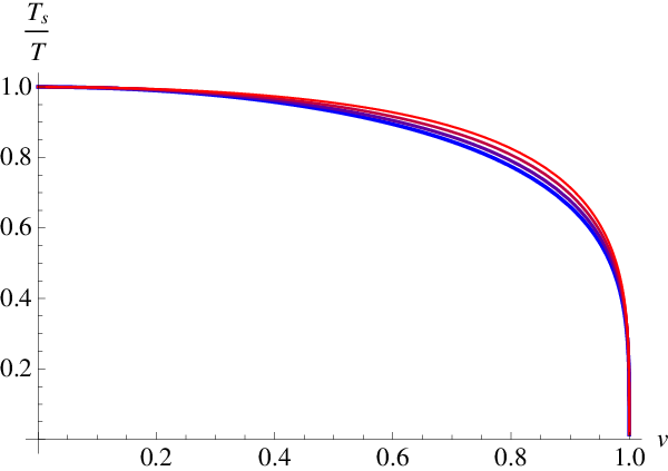
To keep the velocity constant, the momentum absorbed by the charged quark, sitting at the string end-point, is dissipated into the bulk and through the horizon by the trailing part of the string, at a constant rate. It is easy to work out a general expression for the drag force in an arbitrary (dilatonic) background (see also [27] and [26]).
| (47) |


As will be the case for quantities that do not need the D7 brane profile, we can give a result up to second order in
| (48) | |||||
with . Postulating a relativistic dispersion relation of the form for some kinetic mass , and inserting in (44) (with for a stationary solution), the above calculation of the drag force implies knowledge of the joint product of and
| (49) |
In the unflavored case, dual to supersymmetric Yang Mills theory, a value of was obtained that was independent both of the mass and of the velocity of the quark
| (50) |
a fact that contradicts the weak coupling prediction [28]. From (48) and (50) we see that, in the flavored background, acquires a logarithmic dependence on the velocity. The product is related to the quark diffusion constant:
| (51) |
where, as mentioned above, is the correct temperature to be used here. Of course this is only true if the Langevin equation is a realistic description of the difusion phenomenon. In fig. 6 we see the modification of this constant with the flavor density . In summary, fundamental flavors contribute more than adjoint matter to the drag force and they inhibit more the diffusion
| (52) | |||||
The friction coefficient is related to the relaxation time . In order to disentangle from the authors of [9] propose to consider a different kind of experiment, in which the string momentum decays exponentially to zero in the absence of drag. Then in (44) implies that for the probe quark. In the string picture this involves a quasinormal mode computation: the string has to fulfill outgoing boundary conditions at the horizon, and Neumann ones at the D7 brane. This cannot be done analytically for generic masses and, by construction, it only yields in the slow limit.


By solving analytically the limit of small masses (), the authors of [9] postulated the existence of an upper bound for the friction coefficient
| (53) |
For nonzero flavor density, we observe from figure 7, that the friction coefficient is decreased and, in particular, the bound is respected.
Combining the knowledge of with that of previously calculated in (49) allows to solve for the kinetic mass. This is, by definition, velocity independent, and should only depend upon the bare mass . The result is shown in the plot 8. Both the constituent mass, and the kinetic mass, increase as the flavor density is switched on. The blue curves were obtained in [9] and the continuous (dashed) blue curve represents the kinetic mass (constituent mass ) at zero flavor density. is a monotonous function of which has a minimum, for at . The purple curves plot the same magnitudes for . These curves are only trustable in this interval of masses.
8 Jet quenching
The jet quenching parameter measures the momentum broadening of a quark traversing the quark-gluon plasma. If we assume that the heavy quark undergoes a Langevin diffusion process inside the plasma, the diffusion constant associated to this process is simply related to the jet quenching parameter. At a classical level, the Langevin diffusion reduces to an ordinary diffusion process.
The Langevin quantum description implies the presence of a stochastic force acting on the quark, both in the direction longitudinal and transverse to the motion of the quark. Let us denote the two components of this force by respectively. The two-point correlator of this force defines the diffusion constant . Namely, at sufficiently long times (with respect to the typical correlation time of the medium, roughly the inverse temperature), we can write , for each longitudinal and transverse direction.
As it has been shown [29], this allows to determine the momentum broadening of the quark in terms of the diffusion constant. We adopt the definition of the jet quenching parameter as the average momentum squared of the quark divided by the distance the quark has travelled, . Keeping in mind the definition of the diffusion constant, the average momentum squared in the longitudinal and transverse directions can be obtained in terms of and respectively. This means that, for large enough times , the quark acquires a transverse momentum that averages to zero but has quantum fluctuations . The longitudinal momentum has a classical part related to the drag force and quantum fluctuations from the stochastic force .
The diffusion constants can be computed holographically using the prescription for the holographic retarded correlators [30]. In fact, they are given by the zero frequency limit of the imaginary part of the retarded correlator, . The procedure implies finding the solution for the trailing string fluctuations with appropriate boundary conditions and evaluate the bulk-to-boundary correlator that, in turn, yields the retarded correlator. We apply the steps of [29, 31, 25], where the authors obtained the diffusion constants for the plasma, to the background with backreacted flavors. The aim of this section is to compute the jet quenching parameters in the flavored background using the following formulae:
| (54) |
In order to compute the retarded correlator corresponding from the trailing string, the string ansatz must include the quantum fluctuations
| (55) |
By a change in the time coordinate , with [32], we obtain a quadratic action for the fluctuations with no mixed terms
| (56) |
with
and
| (60) | |||||
| (61) |
Here the subscript indicates functions evaluated at the worldsheet horizon . The retarded correlator is then obtained as
| (62) |
where is the retarded solution to the fluctuation equation, , with boundary conditions given by , at the boundary, and , at the worldsheet horizon. The fact that the fluctuations behave like infalling waves with temperature at the worldsheet horizon implies that appears in the aforementioned Einstein relation.
In fixing the boundary normalization condition, we assume that the fluctuation has a regular expansion in the UV. By this we mean that for large radii the leading behavior of is constant. Indeed, using the expressions (9)-(10) and expanding for a large enough such that , we arrive to the expected expansion for the wave function: . The normalization condition can be set at a cutoff radius (related to the probe quark mass by equation (29)). This avoids the problem of going beyond the truncated expansion in for the bulk fields and we can stay in the regime where . Moreover, the zero frequency limit of is independent of this cutoff. Hence we can consistently derive the diffusion constants (and consequently the jet quenching parameters) with a cutoff and arrive to a final cutoff-independent result.
In order to compute the zero frequency limit of the imaginary part of the retarded correlator we do not need the full solution, but only its asymptotics. Moreover, since is a conserved flux, it can be evaluated at an arbitrary point in the radial coordinate (not necessarily at the boundary). In particular, it is easier to evaluate it at the horizon, using the in-falling wave function expression . Substituting this asymptotic into the formula (62) for the retarded correlator and reminding the definition of the diffusion constant, we obtain
| (63) |
with defined by
| (64) |
The constant is evaluated by matching the low frequency limit of the retarded solution with the exact zero frequency solution and imposing the normalization condition. Summarizing the results of this computation, we get . Moreover, deriving the asymptotics of equation (8), we obtain and similarly for . Therefore, the diffusion constants and jet quenching parameters read
| (65) | |||||
| (66) | |||||
Here we used the asymptotic expansion of the background metric component and the relation between and . We remind that this expansion is valid as long as the velocity satisfies .
 |
 |
 |
 |
The corrections coming from the flavor backreaction in are the same as for the drag force with the addition of corrections coming from the worldsheet temperature in equation (96). We conclude that the jet quenching parameter related to the transverse momentum broadening in the flavored background is increased with respect to the value it takes in the unflavored background. The same conclusion applies to the momentum acquired in the longitudinal direction, since also for the corrections are always positive. Visually, this is shown in the plots of figure 9, where the ratio of the diffusion constants (equivalently the ratio of the jet quenching parameters) is represented.
In figure 10 the jet quenching parameters are plotted, relative to the transverse directions and the longitudinal direction respectively.
The Einstein relation in terms of the jet quenching parameter and the drag force can be written as
where we have to use the worldsheet temperature. This relation is well known to be valid in the supergravity dual, as well as in dilaton-gravity models such as [32], and remains unchanged in the backreacted background, order by order in .
9 Conclusions
The physics of quarks propagating through dense media is a subject of intense research nowadays. The fact that this problem, most probably, involves QCD at strong coupling implies a challenge to the traditional perturbative methods. Holography provides a valuable tool, in spite of the fact that the gravity dual model is only qualitatively related to quantum chromodynamics. The traditional objections to the presence of supersymmetry are bypassed at finite temperature, where supersymmetry is indeed broken. In the present work we have analyzed the properties of probes on a background that was constructed some time ago [1]. This background is analytic. However, the price to pay is that it is a perturbative deformation in powers of a parameter which is roughly the Veneziano parameter . The use of this dual geometry only makes sense in the spirit of effective field theory. The background comes with a cutoff , beyond which the predictions blow up because of the presence of a Landau pole. Conversely all the physical predictions at scales much lower than the cutoff are robust and unique up to corrections which die off with powers of . In the present context, the lowest cutoff energy that one can consider is given by the plasma temperature (or the horizon radius ). When examining the physics in the furthest possible IR, it makes sense to discard the UV corrections, or equivalently send , and work with the effective metric written in (6)-(10). To make sense of the analytic expansion in terms of the parameter , related to the Veneziano factor, the effective energy bound is . This implies that the mass of the quark probes cannot be taken to be very large, namely the relevant range for masses is GeV.
Given all this, and moreover, that among all possible “conifold like” models we have chosen the simplest one, namely , we shall only trust qualitatively our results. At a practical level this amounts to finding the sign of the first order correction to physically motivated quantities. Whether it is positive, negative or vanishing is all we can say within the present effective approach. Of course, as emphasized in the text, there is not a unique prescription as to what two theories should be compared. The choice both here and in [1], [2] has been to keep the total amount of degrees of freedom constant, as measured by the energy density. Using the entropy density would have given qualitatively equivalent results. The phenomenological outcome of this work can be summarized in few sentences. The effective thermal masses (constituent and kinetic ) increase in a flavored theory as compared with their values in an unflavored one. The meson melting transition occurs at a lower value of the ratio . For fixed quark mass this implies a higher temperature. The screening length is also diminished. The conductivity is reduced, which is consistent with the fact that the drag force increases. The flavor diffusion constant is lowered, but the broadening of jets, as parametrized by the jet quenching parameter, is enhanced. All in all, the consistent picture that arises seems to point out in the direction of saying that the fundamental degrees of freedom, have a larger cross section than the adjoint ones.
Acknowledgments
We would like to thank Aldo Cotrone, Elias Kiritsis, Nick Evans, Carlos Núñez, Francesco Nitti, Ioannis Papadimitriou, Alfonso V. Ramallo and Balt van Rees, for useful conversations and comments.
J.T.’s research is supported by the Netherlands Organization for Scientic Research (NWO) under the FOM Foundation research program. J.M. and L.M. are supported by the MICINN and FEDER (grant FPA2008-01838), the Spanish Consolider-Ingenio 2010 Programme CPAN (CSD2007-00042), and the Xunta de Galicia (Conselleria de Educación and grant INCITE09-206-121-PR).
Appendix A Derivation of the conductivity
We will mimic [16] to obtain the conductivity for the probe D7-brane. To simplify notation let us write for the pullback metric
| (67) |
where represent a 3-sphere wrapped by the probe brane, and the pullback metric components are related to the background 10d components given by
| (68) | |||||
| (69) |
We have field strength where, as explained in the main text, the gauge field is given by .
The action for the probe brane has the following form in Einstein frame
| (70) |
where is the induced line element in the Einstein frame, and . When evaluating the determinant in the DBI action, the compact space will factorize since does not take values along these directions, the contribution reads (with )
| (71) |
In this expression we have separated the radial dependence, , from the angular part. Altogether
| (72) |
hence
| (73) |
where , and we have used the factorization of the angular variables to obtain the volume of the 3-sphere, . Notice the length dimensions and .
There are first integrals of motion for , which are holographically related to the charge and current densities
| (74) |
with dimensions , since . Dividing by and defining the quantities and , we can express the radial derivatives of as
| (75) | |||||
| (76) |
One then defines a special locus (which we name singular shell) as the radius such that the numerator in the square root of vanishes, and fixes the value of to make the denominator vanish at the same point, to keep the gauge field real (and, therefore, the Legendre transformed action w.r.t stays real too)
| (77) | |||||
| (78) |
Equation (77) defines implicitely the sigular shell . Notice that for a metric in the form given in (68) we have, from equation (77), that the singular shell and the horizon radius are related by
| (79) |
From equations (77 -78), and using the definitions given in this appendix, we obtain the expression
| (80) |
Which gives the following expression in terms of the bulk components:
| (81) | |||||
Taking the limit is equivalent to taking the limit , where
| (82) |
and also
| (83) |
which gives the result quoted in (37). As a final remark concerning dimensions, notice that for the conductivity, , is consistent with Ohm’s law, since whereas .
Following again the procedure stablished by Karch and O’Bannon in [16] we can study the drag force from the conductivity. For very heavy carriers we expect a classical equation of forced motion
| (84) |
In the stationary situation, with , this will give rise to a steady current
| (85) |
with the density of charge carriers and their velocity. In the very massive probe limit we can discard the first term in the expression (80) and compare it with(85), obtaining
| (86) |
Using this result and the definition of the singular shell (77), as well as the explicit values of the induced metric components in terms of the bulk metric components we find that the velocity and drag force are given by
| (87) |
Appendix B Drag Force and Jet Quenching
Central to the discussion of all these effects is the action for a fundamental string
| (88) |
where the string worldsheet coordinates in the static gauge are labelled by and is the bulk metric in the Einstein frame defined in equation (2), with components given by equation (9). From here the momentum currents can be readily derived
| (89) |
Let us consider first the stationary solution: the ansatz for the classical trailing string reads
| (90) |
where is the velocity of the quark moving along the direction and determines its (steady state) position. The classical on-shell action for the trailing string only depends on the radial derivative of . Therefore, the momentum conjugate to , , is constant along the radial direction. Moreover, is related to the momentum loss of the quark, due to the friction of the medium as the quark is moving in the direction, . This is the drag force that we want to compute.
To proceed, we solve the equation for in terms of the constant and of the background metric. This yields
| (91) |
Reality of this expression is ensured if the denominator and the numerator both change sign simultaneously at the same point defined by
| (92) |
From the first equation and (6) we can solve for in terms of as with . Also, from the second, we have the following implicit expression for the drag force
| (93) |
Comparing (92) and (93) with (87), we find consistency provided .
In order to proceed with the fluctuations it is most convenient to go to a different gauge.
| (94) |
for which the induced metric is diagonal for the same trailing string ansatz as (90)
| (95) |
One sees that is the location of an event horizon of the induced worldsheet metric , for which, performing the standard manipulations one can compute the associated Hawking temperature
| (96) |
from which the result given in (46) follows upon expansion up to second order in This, as usual, defines the worldsheet temperature in terms of the bulk temperature .
In order to compute the jet quenching parameter, we have to resort to the analysis of fluctuations. The ansatz is
| (97) |
Expanding (88) to second order we have (in coordinates)
| (98) |
where the (diagonal) tensors are given in the main text (60) (61). Now we can derive the equations of motion in this gauge. Let
| (99) |
with
or, explicitly,
| (103) |
References
- (1) F. Bigazzi, A. L. Cotrone, J. Mas, A. Paredes, A. V. Ramallo, J. Tarrio, “D3-D7 Quark-Gluon Plasmas,” JHEP 0911, 117 (2009). [arXiv:0909.2865 [hep-th]].
- (2) F. Bigazzi, A. L. Cotrone, J. Mas, D. Mayerson and J. Tarrio, “D3-D7 Quark-Gluon Plasmas at Finite Baryon Density,” arXiv:1101.3560 [hep-th].
- (3) D. Mateos, R. C. Myers and R. M. Thomson, “Thermodynamics of the brane,” JHEP 0705, 067 (2007) [arXiv:hep-th/0701132].
- (4) F. Bigazzi, A. L. Cotrone and J. Tarrio, “Hydrodynamics of fundamental matter,” JHEP 1002 (2010) 083 [arXiv:0912.3256 [hep-th]].
- (5) D. Mateos, R. C. Myers and R. M. Thomson, “Holographic phase transitions with fundamental matter,” Phys. Rev. Lett. 97, 091601 (2006) [hep-th/0605046].
- (6) A. Karch and A. O’Bannon, “Chiral transition of N=4 super Yang-Mills with flavor on a 3-sphere,” Phys. Rev. D 74, 085033 (2006) [hep-th/0605120].
- (7) C. Hoyos, “Higher dimensional conformal field theories in the Coulomb branch,” Phys. Lett. B 696, 145 (2011) [arXiv:1010.4438 [hep-th]].
- (8) T. Albash and C. V. Johnson, “Dynamics of Fundamental Matter in N=2* Yang-Mills Theory,” JHEP 1104, 012 (2011) [arXiv:1102.0554 [hep-th]].
- (9) C. P. Herzog, A. Karch, P. Kovtun, C. Kozcaz and L. G. Yaffe, “Energy loss of a heavy quark moving through N = 4 supersymmetric Yang-Mills plasma”, JHEP 0607, 013 (2006) [arXiv:hep-th/0605158].
- (10) A. Karch, A. O’Bannon and K. Skenderis, “Holographic renormalization of probe D-branes in AdS/CFT,” JHEP 0604, 015 (2006) [arXiv:hep-th/0512125].
- (11) V. G. Filev and D. Zoakos, “Towards Unquenched Holographic Magnetic Catalysis,” JHEP 1108, 022 (2011) [arXiv:1106.1330 [hep-th]].
- (12) B. C. van Rees, “Holographic renormalization for irrelevant operators and multi-trace counterterms,” JHEP 1108, 093 (2011) [arXiv:1102.2239 [hep-th]].
- (13) I. Papadimitriou, “Holographic Renormalization of general dilaton-axion gravity,” JHEP 1108, 119 (2011) [arXiv:1106.4826 [hep-th]].
- (14) T. Albash, V. G. Filev, C. V. Johnson and A. Kundu, “Finite temperature large N gauge theory with quarks in an external magnetic field,” JHEP 0807, 080 (2008) [arXiv:0709.1547 [hep-th]].
- (15) J. Erdmenger, R. Meyer and J. P. Shock, “AdS/CFT with flavour in electric and magnetic Kalb-Ramond fields,” JHEP 0712, 091 (2007) [arXiv:0709.1551 [hep-th]].
- (16) A. Karch and A. O’Bannon, “Metallic AdS/CFT,” JHEP 0709, 024 (2007) [arXiv:0705.3870 [hep-th]].
- (17) J. M. Maldacena, “Wilson loops in large N field theories,” Phys. Rev. Lett. 80, 4859 (1998) [hep-th/9803002].
- (18) S. -J. Rey and J. -T. Yee, “Macroscopic strings as heavy quarks in large N gauge theory and anti-de Sitter supergravity,” Eur. Phys. J. C 22, 379 (2001) [hep-th/9803001].
- (19) S. -J. Rey, S. Theisen and J. -T. Yee, “Wilson-Polyakov loop at finite temperature in large N gauge theory and anti-de Sitter supergravity,” Nucl. Phys. B 527, 171 (1998) [hep-th/9803135].
- (20) A. Brandhuber, N. Itzhaki, J. Sonnenschein and S. Yankielowicz, “Wilson loops in the large N limit at finite temperature,” Phys. Lett. B 434, 36 (1998) [hep-th/9803137].
- (21) F. Bigazzi, A. L. Cotrone and A. Paredes, “Klebanov-Witten theory with massive dynamical flavors,” JHEP 0809, 048 (2008) [arXiv:0807.0298 [hep-th]].
- (22) E. V. Shuryak, “What RHIC experiments and theory tell us about properties of quark-gluon plasma?,” Nucl. Phys. A 750, 64 (2005) [arXiv:hep-ph/0405066].
- (23) R. Baier, Y. L. Dokshitzer, A. H. Mueller, S. Peigne and D. Schiff, “Radiative energy loss and p(T)-broadening of high energy partons in nuclei,” Nucl. Phys. B 484, 265 (1997) [arXiv:hep-ph/9608322].
- (24) H. Liu, K. Rajagopal and U. A. Wiedemann, “Calculating the jet quenching parameter from AdS/CFT”, Phys. Rev. Lett. 97, 182301 (2006) [arXiv:hep-ph/0605178].
- (25) G. C. Giecold, E. Iancu and A. H. Mueller, “Stochastic trailing string and Langevin dynamics from AdS/CFT,” JHEP 0907, 033 (2009) [arXiv:0903.1840 [hep-th]].
- (26) U. Giecold, E. Kiritsis, G. Michalogiorgakis and F. Nitti, “Thermal Transport and Drag Force in Improved Holographic QCD,” JHEP 0912 (2009) 056 [arXiv:0906.1890] [hep-ph].
- (27) C. P. Herzog, “Energy loss of heavy quarks from asymptotically AdS geometries,” JHEP 0609, 032 (2006) [arXiv:hep-th/0605191].
- (28) G. D. Moore and D. Teaney, “How much do heavy quarks thermalize in a heavy ion collision?,” Phys. Rev. C 71, 064904 (2005) [hep-ph/0412346].
- (29) S. S. Gubser, “Momentum fluctuations of heavy quarks in the gauge-string duality,” Nucl. Phys. B 790 (2008) 175 [arXiv:hep-th/0612143].
- (30) C. P. Herzog and D. T. Son, “Schwinger-Keldysh propagators from AdS/CFT correspondence,” JHEP 0303, 046 (2003) [arXiv:hep-th/0212072].
- (31) J. Casalderrey-Solana and D. Teaney, “Transverse momentum broadening of a fast quark in a N = 4 Yang Mills plasma,” JHEP 0704 (2007) 039 [arXiv:hep-th/0701123].
- (32) U. Gursoy, E. Kiritsis, L. Mazzanti and F. Nitti, “Langevin diffusion of heavy quarks in non-conformal holographic backgrounds,” JHEP 1012, 088 (2010) [arXiv:1006.3261 [hep-th]].