跳到论文正文
W Papers独立论文阅读器 arXiv:1205.6107 论文正文 计算阅读时间 · 0%
引用这篇论文根据当前论文元数据生成,正式投稿前建议核对。


License: arXiv.org perpetual non-exclusive license
arXiv:1205.6107v1 [math.NA] 28 May 2012

Ghost Force Influence of a Quasicontinuum Method in Two DimensionThanks: The work of Ming was partially supported by National Natural Science Foundation of China grants 10932011, by the funds from Creative Research Groups of China through grant 11021101, and by the support of CAS National Center for Mathematics and Interdisciplinary Sciences. The authors are grateful to Weinan E and Jianfeng Lu for helpful discussions.

Jingrun Chen Address: Institute of Computational Mathematics and Scientific/Engineering Computing, AMSS, Chinese Academy of Sciences, No. 55, Zhong-Guan-Cun East Road, Beijing, 100190, China Email address: chenjr@lsec.cc.ac.cn Current address: South Hall 6705, Mathematics Department, University of California, Santa Barbara, CA93106, USA Email address: cjr@math.ucsb.edu and Pingbing Ming Address: LSEC, Institute of Computational Mathematics and Scientific/Engineering Computing, AMSS, Chinese Academy of Sciences, No. 55 Zhong-Guan-Cun East Road, Beijing, 100190, China Email address: mpb@lsec.cc.ac.cn
Date: August 24, 2026
Abstract.

We derive an analytical expression for the solution of a two-dimensional quasicontinuum method with a planar interface. The expression is used to prove that the ghost force may lead to a finite size error for the gradient of the solution. We estimate the width of the interfacial layer induced by the ghost force is of 𝒪⁡(ε)\mathcal{O}(\sqrt{\varepsilon}\,) with ε\varepsilon the equilibrium bond length, which is much wider than that of the one-dimensional problem.

Key words and phrases: 
Quasicontinuum method, ghost force, interfacial layer
2000 Mathematics Subject Classification
65N30, 65N12, 65N06, 74G20, 74G15

1. Introduction

Multiscale methods have been developed to simulate mechanical behaviors of solids for several decades [14]. Combination of models at different scales greatly enhances the dimension of problems that computers can deal with. However, problems regarding the consistency, stability and convergence of the multiscale methods may arise from the coupling [3]. Taking the quasicontinuum (QC) method [17, 10] for example, one of the main issues is the so called ghost force problem [16], which is the artificial non-zero force that the atoms experience at the equilibrium state. In the language of numerical analysis, the scheme lacks consistency at the interface between the atomistic region and the continuum region [4]. For the one-dimensional problem, it has been shown in [15] that the ghost force may lead to a finite size error for the gradient of the solution. This generates an interfacial layer with width 𝒪⁡(ε​|ln⁡ε|)\mathcal{O}(\varepsilon\lvert\ln\varepsilon\rvert), out of which the error for the gradient of the solution is of 𝒪⁡(ε)\mathcal{O}(\varepsilon).

To understand the influence of the ghost force for high dimensional problems, we study a two-dimensional triangular lattice model with a QC approximation. This QC method couples the Cauchy-Born elasticity model and the atomistic model with a planar interface. Numerical results show that the ghost force may lead to a finite size error for the gradient of the solution as in the one-dimensional problem. The error profile exhibits a layer-like structure. It seems that the width of the interfacial layer induced by the ghost force is of 𝒪⁡(ε)\mathcal{O}(\sqrt{\varepsilon}), which is much wider than that of the one-dimensional problem.

To further characterize the influence of the ghost force, we introduce a square lattice model with a QC approximation. Compared to the triangular lattice model, this model can be solved analytically and the error profile exhibits a clear layer-like structure. Based on the analytical solution, we prove the error committed by the ghost force for the gradient of the solution is 𝒪⁡(1)\mathcal{O}(1) and the width of the induced interfacial layer is of 𝒪⁡(ε)\mathcal{O}(\sqrt{\varepsilon}), which are also confirmed by the numerical results.

The paper is organized as follows. Numerical results for the triangular model and the square lattice model with QC approximations are presented in § 2 and § 3, respectively. We derive an analytical expression of the solution of the square lattice model with a QC approximation in § 4. The main results of the paper are proved in § 5.

2. A quasicontinuum method for triangular lattice

2.1. Atomistic and continuum models

We consider the triangular lattice 𝕃\mathbb{L}, which can be written as

𝕃={x∈ℝ2∣x=ma1+na2,m,n∈ℤ}\mathbb{L}=\{\,x\in\mathbb{R}^{2}\,\mid\,x=ma_{1}+na_{2},\;m,n\in\mathbb{Z}\,\}

with the basis vectors a1=(1,0),a2=(1/2,3/2)a_{1}=(1,0),a_{2}=(1/2,\sqrt{3}/2). Define the unit cell of 𝕃\mathbb{L} as

Γ={x∈ℝ2∣x=c1a1+c2a2,−1/2≤c1,c2<1/2}.\Gamma=\{\,x\in\mathbb{R}^{2}\,\mid\,x=c_{1}a_{1}+c_{2}a_{2},\;-1/2\leq c_{1},c_{2}<1/2\,\}.

We shall consider lattice system ε​𝕃\varepsilon\mathbb{L} inside the domain Ω\Omega, and Ωε=Ω∩ε​𝕃\Omega_{\varepsilon}=\Omega\cap\varepsilon\mathbb{L}, where ε\varepsilon is the equilibrium bond length. Assume that the atoms are interacted with the potential function VV, which is usually a highly nonlinear function, e.g., the Lennard-Jones potential [12]. Denote by 𝒮1\mathcal{S}_{1} and 𝒮2\mathcal{S}_{2} the first and the second neighborhood interaction ranges; see Figure 1. In particular, we have

𝒮1\displaystyle\mathcal{S}_{1} =∪i=16si={a1,a2,−a1+a2,−a1,−a2,a1−a2},\displaystyle=\cup_{i=1}^{6}s_{i}=\{a_{1},a_{2},-a_{1}+a_{2},-a_{1},-a_{2},a_{1}-a_{2}\},
𝒮2\displaystyle\mathcal{S}_{2} =∪i=712si={a1+a2,−a1+2a2,−2a1+a2,−a1−a2,a1−2a2,2a1−a2}.\displaystyle=\cup_{i=7}^{12}s_{i}=\{a_{1}+a_{2},-a_{1}+2a_{2},-2a_{1}+a_{2},-a_{1}-a_{2},a_{1}-2a_{2},2a_{1}-a_{2}\}.

For μ∈ℤ2\mu\in\mathbb{Z}^{2}, the translation operator TεμT^{\mu}_{\varepsilon} is defined for any lattice function z:𝕃→ℝ2z:\mathbb{L}\to\mathbb{R}^{2} as

(Tεμ​z)​(x)=z⁡(x+ε​μ1​a1+ε​μ2​a2)for ​x∈𝕃.(T^{\mu}_{\varepsilon}z)(x)=z(x+\varepsilon\mu_{1}a_{1}+\varepsilon\mu_{2}a_{2})\quad\text{for }x\in\mathbb{L}.

We define the forward and backward discrete gradient operators as

Ds+=ε−1​(Tεμ−I)andDs−=ε−1​(I−Tεμ),D_{s}^{+}=\varepsilon^{-1}(T^{\mu}_{\varepsilon}-I)\qquad\text{and}\qquad D_{s}^{-}=\varepsilon^{-1}(I-T^{\mu}_{\varepsilon}),

where s=μ1​a1+μ2​a2s=\mu_{1}a_{1}+\mu_{2}a_{2} and II is the identity operator. We shall also use the short-hand D​z=(D1+​z,D2+​z)=(Ds1+​z,Ds2+​z)Dz=(D_{1}^{+}z,D_{2}^{+}z)=(D_{s_{1}}^{+}z,D_{s_{2}}^{+}z).

Refer to caption
Figure 1. The first and second neighborhood interaction ranges of the triangular lattice; 𝒮1={s1,⋯,s6}\mathcal{S}_{1}=\{s_{1},\cdots,s_{6}\} and 𝒮2={s7,⋯,s12}\mathcal{S}_{2}=\{s_{7},\cdots,s_{12}\}.

Consider an atomic system posed on Ωε\Omega_{\varepsilon}. The total energy is given by

(2.1) Eattot=12​∑x∈Ωε∑s∈𝒮1∪𝒮2V⁡(|Ds+​z​(x)|),E^{\text{tot}}_{\text{at}}=\dfrac{1}{2}\sum_{x\in\Omega_{\varepsilon}}\sum_{s\in\mathcal{S}_{1}\cup\mathcal{S}_{2}}V\left(\lvert D_{s}^{+}z(x)\rvert\right),

where VV is a potential function. In this paper, we only consider the pairwise potential function, and leave the discussion on the more general potential functions in future publication. The atomistic problem is to minimize the total energy subject to certain boundary conditions that will be specified later on.

Next we turn to the Cauchy-Born elasticity model [1, 6, 5, 7]. Given a 22 by 22 matrix AA, the stored energy density function is given by

Wcb​(A)=12​ϑ0​∑s∈𝒮1∪𝒮2V⁡(|s⋅A|),W_{\text{cb}}(A)=\dfrac{1}{2\vartheta_{0}}\sum_{s\in\mathcal{S}_{1}\cup\mathcal{S}_{2}}V(\lvert s\cdot A\rvert),

where ϑ0\vartheta_{0} is the area of the unit cell and ϑ0=3​ε2/2\vartheta_{0}=\sqrt{3}\varepsilon^{2}/2. The stored energy function is defined by

Ecbtot=∫ΩWcb​(∇z​(x))​𝑑x.E^{\text{tot}}_{\text{cb}}=\int_{\Omega}W_{\text{cb}}(\nabla z(x))\,\mathrm{d}\,x.

The continuum problem is to minimize the stored energy function subject to certain boundary conditions. We employ the standard P1P_{1} Lagrange finite element to approximate the Cauchy-Born elasticity model with the lattice 𝕃\mathbb{L} as the triangulation. The approximate stored energy function is

(2.2) Ecb,εtot=12​∑x∈Ωε∑i=16(V⁡(|Dsi+​z​(x)|)+V⁡(|(Dsi++Dsi+1+)​z​(x)|)).E^{\text{tot}}_{\text{cb},\varepsilon}=\dfrac{1}{2}\sum_{x\in\Omega_{\varepsilon}}\sum_{i=1}^{6}\left(V\left(\lvert D_{s_{i}}^{+}z(x)\rvert\right)+V\left(\lvert(D_{s_{i}}^{+}+D_{s_{i+1}}^{+})z(x)\rvert\right)\right).

One can see Ecb,εtotE^{\text{tot}}_{\text{cb},\varepsilon} reproduces the atomistic energy EattotE^{\text{tot}}_{\text{at}}; cf. (2.1), if only the nearest neighborhood interaction is considered.

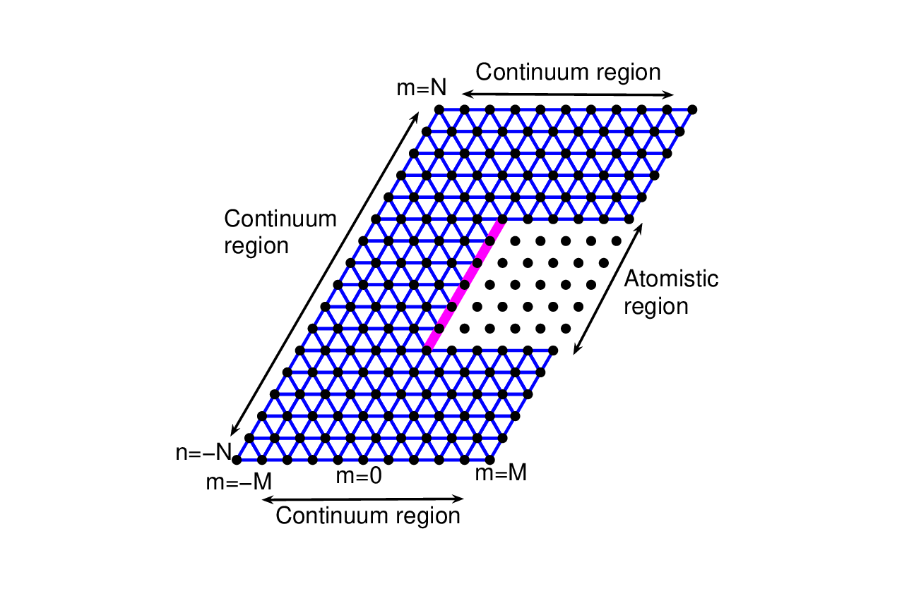
We study the quasicontinuum method [17]. Let ε=1/(2​M)\varepsilon=1/(2M). We assume that the interface between the continuum model and the atomistic model is x1=0x_{1}=0 as shown in Figure 2. The total energy of the QC method is

Eqctot\displaystyle E^{\text{tot}}_{\text{qc}} =12​∑x1≤−2​ε∑i=16(V⁡(|Dsi+​z​(x)|)+V⁡(|(Dsi++Dsi+1+)​z​(x)|))\displaystyle=\dfrac{1}{2}\sum_{x_{1}\leq-2\varepsilon}\sum_{i=1}^{6}\left(V\left(\lvert D_{s_{i}}^{+}z(x)\rvert\right)+V\left(\lvert(D_{s_{i}}^{+}+D_{s_{i+1}}^{+})z(x)\rvert\right)\right)
+12∑x1=−ε{∑i=16(V(|Dsi+z(x)|)+V(|(Dsi++Dsi+1+)z(x)|))+V(|Ds12+z(x)|)}\displaystyle\quad+\dfrac{1}{2}\sum_{x_{1}=-\varepsilon}\bigg\{\sum_{i=1}^{6}\left(V\left(\lvert D_{s_{i}}^{+}z(x)\rvert\right)+V\left(\lvert(D_{s_{i}}^{+}+D_{s_{i+1}}^{+})z(x)\rvert\right)\right)+V(\lvert D_{s_{12}}^{+}z(x)\rvert)\bigg\}
+12∑x1=0{∑s∈𝒮1V(|Ds+z(x)|)+∑i=24(V(|Dsi+z(x)|)+V(|(Dsi++Dsi+1+)z(x)|))\displaystyle\quad+\dfrac{1}{2}\sum_{x_{1}=0}\bigg\{\sum_{s\in\mathcal{S}_{1}}V\left(\lvert D_{s}^{+}z(x)\rvert\right)+\sum_{i=2}^{4}\left(V\left(\lvert D_{s_{i}}^{+}z(x)\rvert\right)+V\left(\lvert(D_{s_{i}}^{+}+D_{s_{i+1}}^{+})z(x)\rvert\right)\right)
+12V(|Ds7+z(x)|)+V(|Ds11+z(x)|)+V(|Ds12+z(x)|)}\displaystyle\phantom{+\dfrac{1}{2}\sum_{x_{1}=0}\bigg\{}\qquad+\dfrac{1}{2}V(\lvert D_{s_{7}}^{+}z(x)\rvert)+V(\lvert D_{s_{11}}^{+}z(x)\rvert)+V(\lvert D_{s_{12}}^{+}z(x)\rvert)\bigg\}
+12∑x1=ε{∑s∈𝒮1∪𝒮2V(|Ds+z(x)|)−12V(|Ds9+z(x)|)}\displaystyle\quad+\dfrac{1}{2}\sum_{x_{1}=\varepsilon}\bigg\{\sum_{s\in\mathcal{S}_{1}\cup\mathcal{S}_{2}}V\left(\lvert D_{s}^{+}z(x)\rvert\right)-\dfrac{1}{2}V(\lvert D_{s_{9}}^{+}z(x)\rvert)\bigg\}
+12∑x1≥2​ε∑s∈𝒮1∪𝒮2V(|Ds+z(x)|).\displaystyle\quad+\dfrac{1}{2}\sum_{x_{1}\geq 2\varepsilon}\sum_{s\in\mathcal{S}_{1}\cup\mathcal{S}_{2}}V\left(\lvert D_{s}^{+}z(x)\rvert\right).

The force at atom xx is defined by

ℱqc​[z]​(x)≡−∂Eqctot∂z⁡(x).\mathcal{F}_{\text{qc}}[z](x)\equiv-\dfrac{\partial E^{\text{tot}}_{\text{qc}}}{\partial z(x)}.

Since we only concern the influence of the ghost force, following [15], we assume that the potential function is a harmonic function, i.e.,

V⁡(r)=12​r2.V(r)=\dfrac{1}{2}{r^{2}}.

Without taking into account the external force, we write the equilibrium equations for the QC approximation as

ℱqc​[z]​(x)=0\mathcal{F}_{\text{qc}}[z](x)=0

with

ℱqc​[z]​(x)\displaystyle\mathcal{F}_{\text{qc}}[z](x) =−12​z​(x)+∑i=112z⁡(x+ε​si),\displaystyle=-12z(x)+\sum_{i=1}^{12}z(x+\varepsilon s_{i}), x∈Ωε,x1≤−2​ε,\displaystyle x\in\Omega_{\varepsilon},x_{1}\leq-2\varepsilon,
ℱqc​[z]​(x)\displaystyle\mathcal{F}_{\text{qc}}[z](x) =−24​z​(x)+4​∑i=16z⁡(x+ε​si),\displaystyle=-24z(x)+4\sum_{i=1}^{6}z(x+\varepsilon s_{i}), x∈Ωε,x1≥2​ε.\displaystyle x\in\Omega_{\varepsilon},x_{1}\geq 2\varepsilon.
Refer to caption
Figure 2. Schematic picture of Ωε\Omega_{\varepsilon}.

For x=(−ε,x2)x=(-\varepsilon,x_{2}),

ℱqc​[z]​(x)=−492​z​(x)+4​∑i=16z⁡(x+ε​si)+12​z​(x+ε​s12).\mathcal{F}_{\text{qc}}[z](x)=-\dfrac{49}{2}z(x)+4\sum_{i=1}^{6}z(x+\varepsilon s_{i})+\dfrac{1}{2}z(x+\varepsilon s_{12}).

For x=(0,x2)x=(0,x_{2}),

ℱqc​[z]​(x)\displaystyle\mathcal{F}_{\text{qc}}[z](x) =−18​z​(x)+[z⁡(x+ε​s1)+z⁡(x+ε​s6)]+52​[z⁡(x+ε​s2)+z⁡(x+ε​s5)]\displaystyle=-18z(x)+[z(x+\varepsilon s_{1})+z(x+\varepsilon s_{6})]+\dfrac{5}{2}[z(x+\varepsilon s_{2})+z(x+\varepsilon s_{5})]
+4​[z⁡(x+ε​s3)+z⁡(x+ε​s4)]+[z⁡(x+ε​s7)+z⁡(x+ε​s11)+z⁡(x+ε​s12)].\displaystyle\quad+4[z(x+\varepsilon s_{3})+z(x+\varepsilon s_{4})]+[z(x+\varepsilon s_{7})+z(x+\varepsilon s_{11})+z(x+\varepsilon s_{12})].

For x=(ε,x2)x=(\varepsilon,x_{2}),

ℱqc​[z]​(x)=−232​z​(x)+∑i=112z⁡(x+ε​si)−12​z​(x+ε​s9).\mathcal{F}_{\text{qc}}[z](x)=-\dfrac{23}{2}z(x)+\sum_{i=1}^{12}z(x+\varepsilon s_{i})-\dfrac{1}{2}z(x+\varepsilon s_{9}).

At the equilibrium state, we evaluate ℱqc\mathcal{F}_{\text{qc}} at z⁡(x)=xz(x)=x to get

ℱqc[x](x)={(−3ε/4,3ε/4),ifx1=−ε,(3ε/2,−3ε/2),ifx1=0,(−3ε/4,3ε/4),ifx1=ε,(0,0),otherwise.\mathcal{F}_{\text{qc}}[x](x)=\left\{\begin{aligned} (-3\varepsilon/4,\sqrt{3}\varepsilon/4),&\rm{\quad if\quad}x_{1}=-\varepsilon,\\ (3\varepsilon/2,-\sqrt{3}\varepsilon/2),&\rm{\quad if\quad}x_{1}=0,\\ (-3\varepsilon/4,\sqrt{3}\varepsilon/4),&\rm{\quad if\quad}x_{1}=\varepsilon,\\ (0,0),&\rm{\quad otherwise}.\end{aligned}\right.

The above equations imply z1​(x)=−3​z2​(x)z_{1}(x)=-\sqrt{3}z_{2}(x). Therefore, we only study the first component of z⁡(x)z(x) and neglect the subscript if no confusion will occur. The error of the displacement induced by the ghost force, denoted by y⁡(x)≡z⁡(x)−xy(x)\equiv z(x)-x, satisfies

(2.3) ℱqc​[y]​(x)=ℱqc​[z]​(x)−ℱqc​[x]​(x)=−ℱqc​[x]​(x)≡f⁡(x)\mathcal{F}_{\text{qc}}[y](x)=\mathcal{F}_{\text{qc}}[z](x)-\mathcal{F}_{\text{qc}}[x](x)=-\mathcal{F}_{\text{qc}}[x](x)\equiv f(x)

with

f(x)={3​ε/4, if ​x1=−ε,−3ε/2,ifx1=0,3​ε/4,ifx1=ε,0otherwise.f(x)=\left\{\begin{aligned} 3\varepsilon/4,&\text{\quad if\quad}x_{1}=-\varepsilon,\\ -3\varepsilon/2,&\rm{\quad if\quad}x_{1}=0,\\ 3\varepsilon/4,&\rm{\quad if\quad}x_{1}=\varepsilon,\\ 0&\rm{\quad otherwise}.\end{aligned}\right.

Boundary conditions need to be supplemented to close the system of equilibrium equations. Two types of boundary conditions will be considered in this paper. One is the periodic boundary condition in x2x_{2} direction while homogeneous Dirichlet boundary condition in x1x_{1} direction, which will be called periodic boundary condition if no confusion will occur. The other is the homogeneous Dirichlet boundary conditions in both x1x_{1} and x2x_{2} directions.

In what follows, we shall use a conventional notation y⁡(m,n)=y⁡(x)y(m,n)=y(x) with x=ε⁡(m​a1+n​a2)x=\varepsilon(ma_{1}+na_{2}).

2.2. Periodic boundary condition

The periodic boundary condition can be written as

{y⁡(−M,n)=0,n=−N,⋯,N,y⁡(m,n)=y⁡(m,2​N+n),m=−M,⋯,M,n=−N,⋯,N,y⁡(M,n)=y⁡(M+1,n)=0,n=−N,⋯,N.\left\{\begin{aligned} y(-M,n)&=0,&&n=-N,\cdots,N,\\ y(m,n)&=y(m,2N+n),&&m=-M,\cdots,M,n=-N,\cdots,N,\\ y(M,n)&=y(M+1,n)=0,&&n=-N,\cdots,N.\end{aligned}\right.

Observe that the solution of (2.3) with the periodic boundary condition takes a special form:

y⁡(x)=c​y​(x1),y(x)=cy(x_{1}),

namely, the solution is constant along x2x_{2} direction. Based on this observation, we conclude that the QC approximation with the periodic boundary condition reduces to a one-dimensional problem. The equilibrium equations satisfied by y⁡(x1)y(x_{1}) are as follows. In the continuum region, i.e., m=−M+1,⋯,−2m=-M+1,\cdots,-2,

8​y​(m+1)−16​y​(m)+8​y​(m−1)=0,8y(m+1)-16y(m)+8y(m-1)=0,

and in the atomistic region, i.e., m=2,⋯,M−1m=2,\cdots,M-1,

y⁡(m+2)+4​y​(m+1)−10​y​(m)+4​y​(m−1)+y⁡(m−2)=0.y(m+2)+4y(m+1)-10y(m)+4y(m-1)+y(m-2)=0.

The equations in the interfacial region are

{12​y​(1)+8​y​(0)−332​y​(−1)+8​y​(−2)=34​ε,y⁡(2)+4​y​(1)−13​y​(0)+8​y​(−1)=−32​ε,y⁡(3)+4​y​(2)−192​y​(1)+4​y​(0)+12​y​(−1)=34​ε.\left\{\begin{aligned} \dfrac{1}{2}y(1)+8y(0)-\dfrac{33}{2}y(-1)+8y(-2)&=\dfrac{3}{4}\varepsilon,\\ y(2)+4y(1)-13y(0)+8y(-1)&=-\dfrac{3}{2}\varepsilon,\\ y(3)+4y(2)-\dfrac{19}{2}y(1)+4y(0)+\dfrac{1}{2}y(-1)&=\dfrac{3}{4}\varepsilon.\end{aligned}\right.

The boundary condition is

y⁡(−M)=y⁡(M)=y⁡(M+1)=0.y(-M)=y(M)=y(M+1)=0.

The above equilibrium equations can also be obtained by considering a one-dimensional chain interacted with the following harmonic potential:

(2.4) V⁡({y})=k12​∑|i−j|=1|yi−yj|2+k22​∑|i−j|=2|yi−yj|2V(\{y\})=\dfrac{k_{1}}{2}\sum_{\lvert i-j\rvert=1}\lvert y_{i}-y_{j}\rvert^{2}+\dfrac{k_{2}}{2}\sum_{\lvert i-j\rvert=2}\lvert y_{i}-y_{j}\rvert^{2}

with k1=4k_{1}=4 and k2=1k_{2}=1. This is the model studied in [2].

2.3. Dirichlet boundary condition

The Dirichlet boundary condition can be written as

{y⁡(−M,n)=y⁡(M,n)=y⁡(M+1,n)=0,n=−N,⋯,N,y⁡(m,−N)=y⁡(m,N)=0,m=−M,⋯,−1,y⁡(m,−N−1)=y⁡(m,−N)=y⁡(m,N)=y⁡(m,N+1)=0,m=0,⋯,M.\left\{\begin{aligned} y(-M,n)&=y(M,n)=y(M+1,n)=0,&&n=-N,\cdots,N,\\ y(m,-N)&=y(m,N)=0,&&m=-M,\cdots,-1,\\ y(m,-N-1)&=y(m,-N)=y(m,N)=y(m,N+1)=0,&&m=0,\cdots,M.\end{aligned}\right.

This gives an essentially two-dimensional model. We show profiles of discrete gradients Ds1+​yD_{s_{1}}^{+}y and Ds2+​yD_{s_{2}}^{+}y in Figure 3 with M=N=20M=N=20. The profile of Ds1+​yD_{s_{1}}^{+}y is similar to that of the one-dimensional problem. However, if one zooms in the interface, there are some differences. To highlight the interface, for i=1,2i=1,2, we define

Ei={x∈Ωε∣|Dsi​y​(x)|≥c0​ε},E_{i}=\{\,x\in\Omega_{\varepsilon}\,\mid\,\lvert D_{s_{i}}y(x)\rvert\geq c_{0}\varepsilon\,\},

and let χEi\chi_{E_{i}} be their characteristic functions. We plot χEi​(x)\chi_{E_{i}}(x) in Figure 4 with M=N=640M=N=640 and c0=0.04c_{0}=0.04. In Figure 4(a), the width of the interface near the boundary is much wider than that in the interior domain. No interfacial layer for Ds2+​yD_{s_{2}}^{+}y is observed in Figure 4(b). Therefore, we only measure the width of the interfacial layer for Ds1+​yD_{s_{1}}^{+}y, which is defined by

maxn{|a1|ε\displaystyle\max_{n}\Big\{|a_{1}|\varepsilon [argmaxm{x=ma1ε+na2ε∈Ωε|χ1(x)=1}\displaystyle\big[\operatorname{argmax}_{m}\{x=ma_{1}\varepsilon+na_{2}\varepsilon\in\Omega_{\varepsilon}|\chi_{1}(x)=1\}
−argminm{x=ma1ε+na2ε∈Ωε|χ1(x)=1}]}.\displaystyle-\operatorname{argmin}_{m}\{x=ma_{1}\varepsilon+na_{2}\varepsilon\in\Omega_{\varepsilon}|\chi_{1}(x)=1\}\big]\Big\}.

Numerical results in Table 1 imply that the width of the interfacial layer scales 𝒪⁡(ε)\mathcal{O}(\sqrt{\varepsilon}), while the one-dimensional problem has an interfacial layer with 𝒪⁡(ε​|ln⁡ε|)\mathcal{O}(\varepsilon\lvert\ln\varepsilon\rvert) width [15, 2].

Refer to caption
(a) Ds1+​yD_{s_{1}}^{+}y
Refer to caption
(b) Ds2+​yD_{s_{2}}^{+}y
Figure 3. Profiles of the discrete gradients for triangular lattice with M=N=20M=N=20 under Dirichlet boundary condition.
Refer to caption
(a) χE1​(x)\chi_{E_{1}}(x)
Refer to caption
(b) χE2​(x)\chi_{E_{2}}(x)
Figure 4. Profiles of the characteristic functions for triangular lattice.
ε⁡(5×10⁻²)\varepsilon\;(5\times 10^{-2}) 202^{0} 2−12^{-1} 2−22^{-2} 2−32^{-3} 2−42^{-4} 2−52^{-5} Rate
Layer width(10−1)(10^{-1}) 3.53.5 2.32.3 1.51.5 0.940.94 0.630.63 0.520.52 0.570.57
Table 1. Width of the interfacial layer versus the equilibrium bond length ε\varepsilon for the triangular lattice with Dirichlet boundary condition.

One may doubt the above result could be caused by the boundary condition instead of the ghost force. To clarify this issue, we enlarge the continuum region to weaken the influence of the boundary condition. We set N=3​MN=3M and use different equilibrium equations for different regions as in Figure 5. Roughly speaking, along x2x_{2} direction, the original QC method is employed in the interior region, and the continuum model is padded in the outer region.

Refer to caption
Figure 5. Padding technique to remove the boundary effect.

We plot Ds1+​yD^{+}_{s_{1}}y, Ds2+​yD^{+}_{s_{2}}y, and their characteristic functions in Figure 6 and Figure 7. They are similar to those in Figure 3 and Figure 4.

Refer to caption
(a) Ds1+​yD_{s_{1}}^{+}y
Refer to caption
(b) Ds2+​yD_{s_{2}}^{+}y
Figure 6. Profiles of the discrete gradients for triangular lattice with M=20M=20 and padding technique under Dirichlet boundary condition.
Refer to caption
(a) χE1​(x)\chi_{E_{1}}(x)
Refer to caption
(b) χE2​(x)\chi_{E_{2}}(x)
Figure 7. Profiles of the characteristic functions for triangular lattice with padding technique.

Table 2 shows the width of the interfacial layer in terms of ε\varepsilon. Numerical results suggest that the width of the interfacial layer is still of 𝒪⁡(ε)\mathcal{O}(\sqrt{\varepsilon}\,), which is consistent with that in Table 1. Therefore, we conclude that the interface is caused by the ghost force instead of the boundary condition.

ε⁡(10−2)\varepsilon(10^{-2}) 1.71.7 0.830.83 0.410.41 0.210.21 0.100.10 Rate
Layer width(10−2)(10^{-2}) 9.29.2 8.38.3 4.84.8 3.33.3 2.32.3 0.530.53
Table 2. Width of the interfacial layer versus the equilibrium bond length ε\varepsilon by removing the effect of the boundary condition.

The QC approximation discussed in this section is quite realistic except the potential function as shown in [15], which however seems enough to characterize the influence of the ghost force. Unfortunately, it does not seem easy to solve this model analytically as we have done in [15] for the one-dimensional problem. In next section, we introduce a new QC method that can be solved analytically. We shall prove that this new QC method does capture the main feature of the ghost force for the triangular lattice model with a planar interface.

3. Square lattice model

We consider the square lattice with the harmonic potential. Compared to the standard interaction range of the square lattice, we assume a special interaction range as shown in Figure 8 (Left). Namely, the first and second neighborhood interactions in x1x_{1} direction, and the first neighborhood interaction in x2x_{2} direction are taken into account. This seemingly strange selection may be obtained from a rotated triangular lattice as in Figure 8 (Right). If we condense the interaction of the atoms 9,4,5,119,4,5,11 into one atom, and the atoms 8,2,1,128,2,1,12 into another, then we obtain a square lattice model with the special interaction range described above, which may be the underlying reason why it can be regarded as a surrogate model. We shall show in the next two sections that this model not only captures the main features of the triangular lattice model with the QC approximation as shown in Figure 2, but also lends itself theoretically tractable.

Refer to caption
Refer to caption
Figure 8. Interaction ranges. Left: First and second neighborhood interactions in x1x_{1} direction and first neighborhood interaction in x2x_{2} direction for square lattice; Right: First and second neighborhood interactions for triangular lattice in a rotated coordinate.

Proceeding along the same line that leads to (2.3), we obtain the equilibrium equations for the error y⁡(x)y(x).11 1 We actually multiply −1-1 on both sides of (2.3). In the continuum region, i.e., m=−M,⋯,−2m=-M,\cdots,-2 and n=−N,⋯,Nn=-N,\cdots,N,

12​yi​(m,n)\displaystyle 12y_{i}(m,n) −yi​(m,n−1)−yi​(m,n+1)−5​yi​(m−1,n)−5​yi​(m+1,n)\displaystyle-y_{i}(m,n-1)-y_{i}(m,n+1)-5y_{i}(m-1,n)-5y_{i}(m+1,n)
(3.1) =0,i=1,2,\displaystyle=0,\quad i=1,2,

and in the atomistic region, i.e., m=2,⋯,Mm=2,\cdots,M and n=−N,⋯,Nn=-N,\cdots,N,

6​yi​(m,n)\displaystyle 6y_{i}(m,n) −yi​(m,n−1)−yi​(m,n+1)−yi​(m−1,n)−yi​(m+1,n)\displaystyle-y_{i}(m,n-1)-y_{i}(m,n+1)-y_{i}(m-1,n)-y_{i}(m+1,n)
(3.2) −yi(m−2,n)−yi(m+2,n)=0,i=1,2.\displaystyle-y_{i}(m-2,n)-y_{i}(m+2,n)=0,\quad i=1,2.

The interface between the continuum model and the atomistic model is the line m=0m=0 as shown in Figure 9, and MM is assumed to be even for simplicity. The equilibrium equations for the layers m=−1,0m=-1,0 and 11 are as follows.

Refer to caption
Figure 9. Square lattice with a planar interface.

For layer m=−1m=-1 and n=−N,⋯,Nn=-N,\cdots,N,

252​yi​(−1,n)\displaystyle\frac{25}{2}y_{i}(-1,n) −yi​(−1,n−1)−yi​(−1,n+1)−5​yi​(−2,n)−5​yi​(0,n)\displaystyle-y_{i}(-1,n-1)-y_{i}(-1,n+1)-5y_{i}(-2,n)-5y_{i}(0,n)
(3.3) −12yi(1,n)=fi,i=1,2,\displaystyle-\frac{1}{2}y_{i}(1,n)=f_{i},\quad i=1,2,

where f1=−εf_{1}=-\varepsilon and f2=0f_{2}=0.

For layer m=0m=0 and n=−N,⋯,Nn=-N,\cdots,N,

9​yi​(0,n)\displaystyle 9y_{i}(0,n) −yi​(0,n−1)−yi​(0,n+1)−5​yi​(−1,n)−yi​(1,n)\displaystyle-y_{i}(0,n-1)-y_{i}(0,n+1)-5y_{i}(-1,n)-y_{i}(1,n)
(3.4) −yi(2,n)=fi,i=1,2,\displaystyle-y_{i}(2,n)=f_{i},\quad i=1,2,

where f1=2​εf_{1}=2\varepsilon and f2=0f_{2}=0.

For layer m=1m=1 and n=−N,⋯,Nn=-N,\cdots,N,

112​yi​(1,n)\displaystyle\frac{11}{2}y_{i}(1,n) −yi​(1,n−1)−yi​(1,n+1)−yi​(0,n)−yi​(2,n)\displaystyle-y_{i}(1,n-1)-y_{i}(1,n+1)-y_{i}(0,n)-y_{i}(2,n)
(3.5) −12yi(−1,n)−yi(3,n)=fi,i=1,2,\displaystyle-\frac{1}{2}y_{i}(-1,n)-y_{i}(3,n)=f_{i},\quad i=1,2,

where f1=−εf_{1}=-\varepsilon and f2=0f_{2}=0.

Observe that

y2=0.y_{2}=0.

Therefore, we only consider y1y_{1} and omit the subscript from now on.

We first impose the Dirichlet boundary condition in the x1x_{1} direction, and the periodic boundary condition in the x2x_{2} direction as

(3.6) {y⁡(−M,n)=y(M,n)=y(M+1,n)=0,n=−N,⋯,N,y⁡(m,n)=y(m,n+2N),m=−M,⋯,M,n=−N,⋯,N.\left\{\begin{aligned} y(-M,n)&=y(M,n)=y(M+1,n)=0,\quad n=-N,\cdots,N,\\ y(m,n)&=y(m,n+2N),\quad m=-M,\cdots,M,n=-N,\cdots,N.\end{aligned}\right.

Similar to the triangular lattice model, it is easy to check that the square lattice model reduces to a one-dimensional chain model with the following equilibrium equations and boundary condition.

5​y​(m+1)−10​y​(m)+5​y​(m−1)\displaystyle 5y(m+1)-10y(m)+5y(m-1) =0,m=−M+1,⋯,−2,\displaystyle=0,\;m=-M+1,\cdots,-2,
y⁡(m+2)+y⁡(m+1)−4​y​(m)+y⁡(m−1)+y⁡(m−2)\displaystyle y(m+2)+y(m+1)-4y(m)+y(m-1)+y(m-2) =0,m=2,⋯,M−1.\displaystyle=0,\;m=2,\cdots,M-1.

The equations for the interface are

{12​y​(1)+5​y​(0)−212​y​(−1)+5​y​(−2)=ε,y⁡(2)+y⁡(1)−7​y​(0)+5​y​(−1)=−2​ε,y⁡(3)+y⁡(2)−72​y​(1)+y⁡(0)+12​y​(−1)=ε.\left\{\begin{aligned} \dfrac{1}{2}y(1)+5y(0)-\dfrac{21}{2}y(-1)+5y(-2)&=\varepsilon,\\ y(2)+y(1)-7y(0)+5y(-1)&=-2\varepsilon,\\ y(3)+y(2)-\dfrac{7}{2}y(1)+y(0)+\dfrac{1}{2}y(-1)&=\varepsilon.\end{aligned}\right.

The boundary condition is

y⁡(−M)=y⁡(M)=y⁡(M+1)=0.y(-M)=y(M)=y(M+1)=0.

It is clear that the above model is exactly the same as that has been studied in [15], which can also be obtained from the one-dimensional model (2.4) with k1=k2=1k_{1}=k_{2}=1.

Therefore, we impose the Dirichlet boundary condition in both x1x_{1} and x2x_{2} directions as follows.

(3.7) {y⁡(−M,n)=y⁡(M,n)=y⁡(M+1,n)=0,n=−N,⋯,N,y⁡(m,−N)=y⁡(m,N)=0,m=−M,⋯,M.\left\{\begin{aligned} y(-M,n)&=y(M,n)=y(M+1,n)=0,&&n=-N,\cdots,N,\\ y(m,-N)&=y(m,N)=0,&&m=-M,\cdots,M.\end{aligned}\right.

Choosing M=N=20M=N=20, we show profiles of the discrete gradients Ds1+​yD_{s_{1}}^{+}y and Ds2+​yD_{s_{2}}^{+}y in Figure 10. The feature is similar to that of the triangular lattice model. To highlight the interface, we plot the characteristic functions χE1\chi_{E_{1}} and χE2\chi_{E_{2}} in Figure 11 with M=N=320M=N=320 and c0=0.04c_{0}=0.04.

Refer to caption
(a) Ds1+​yD_{s_{1}}^{+}y
Refer to caption
(b) Ds2+​yD_{s_{2}}^{+}y
Figure 10. Profiles of the discrete gradients of yy for square lattice with M=N=20M=N=20 under Dirichlet boundary condition.
Refer to caption
(a) χE1​(x)\chi_{E_{1}}(x)
Refer to caption
(b) χE2​(x)\chi_{E_{2}}(x)
Figure 11. Profiles of the characteristic functions for square lattice.

We report the width of the interfacial layer in Table 3. It is clear that the width of the interfacial layer is of 𝒪⁡(ε)\mathcal{O}(\sqrt{\varepsilon}\,), which is consistent with that of the triangular lattice. In § 5, we shall prove this fact.

ε⁡(5×10⁻²)\varepsilon\;(5\times 10^{-2}) 202^{0} 2−12^{-1} 2−22^{-2} 2−32^{-3} 2−42^{-4} Rate
Layer width(10−1)\;(10^{-1}) 88 5.55.5 3.633.63 2.562.56 1.841.84 0.530.53
Table 3. Width of interfacial layer versus the equilibrium bond length ε\varepsilon for square lattice.

4. Exact solution for the square lattice model

To find the exact solution of the QC approximation (3.1) – (3.5) with Dirichlet boundary condition (3.7), we follow the approach in [15]: firstly, we find the general expression for the solution of the continuum equation and the atomistic equation by separation of variables ansatz, with certain unspecified constants; secondly, we use the equations around the interface to determine these constants. The next lemma gives the general expression of the solution.

Lemma 4.1.

For m=−M,⋯,−1m=-M,\cdots,-1 and n=−N,⋯,Nn=-N,\cdots,N, we have

(4.1) y⁡(m,n)=∑k=12​N−1ak​sinh⁡[(M+m)​αk]​sin⁡k​π2​N​(N+n),y(m,n)=\sum_{k=1}^{2N-1}a_{k}\sinh[(M+m)\alpha_{k}]\sin\dfrac{k\pi}{2N}(N+n),

where

cosh⁡αk=1+λk5,λk=2​sin2⁡k​π4​N.\cosh\alpha_{k}=1+\dfrac{\lambda_{k}}{5},\qquad\lambda_{k}=2\sin^{2}\dfrac{k\pi}{4N}.

For m=0,⋯,Mm=0,\cdots,M and n=−N,⋯,Nn=-N,\cdots,N, we have

(4.2) y⁡(m,n)=∑k=12​N−1(bk​(−1)m​Fm​(γk,δk)+ck​fm​(γk,δk))​sin⁡k​π2​N​(N+n),y(m,n)=\sum_{k=1}^{2N-1}\left(b_{k}\bigl(-1\bigr)^{m}F_{m}(\gamma_{k},\delta_{k})+c_{k}f_{m}(\gamma_{k},\delta_{k})\right)\sin\dfrac{k\pi}{2N}(N+n),

where

(4.3) cosh⁡γk=1+25+8​λk4,cosh⁡δk=−1+25+8​λk4,\cosh\gamma_{k}=\dfrac{1+\sqrt{25+8\lambda_{k}}}{4},\quad\cosh\delta_{k}=\dfrac{-1+\sqrt{25+8\lambda_{k}}}{4},

and

(4.4) {Fm​(γ,δ)=sinh⁡[(M+1−m)​γ]+sinh⁡[(M−m)​γ]​cosh⁡δcosh⁡γ+cosh⁡δ−(−1)m​cosh⁡[(M−m)​δ]​sinh⁡γcosh⁡γ+cosh⁡δ,fm​(γ,δ)=Fm​(δ,γ).\left\{\begin{aligned} F_{m}(\gamma,\delta)&=\dfrac{\sinh[(M+1-m)\gamma]+\sinh[(M-m)\gamma]\cosh\delta}{\cosh\gamma+\cosh\delta}\\ &\quad-\bigl(-1\bigr)^{m}\dfrac{\cosh[(M-m)\delta]\sinh\gamma}{\cosh\gamma+\cosh\delta},\\ f_{m}(\gamma,\delta)&=F_{m}(\delta,\gamma).\end{aligned}\right.

The coefficients bkb_{k} and ckc_{k} are parameters to be determined; See; cf., (4.13).

Proof.

By separation of variables, we get (4.1).

The explicit expression for the solution of the atomistic model can also be obtained by separation of variables ansatz. Substituting y⁡(m,n)=f⁡(m)​g​(n)y(m,n)=f(m)g(n) into (3.2), we get

∑i=−22[f⁡(m+i)−f⁡(m)]​g​(n)+∑i=−11[g⁡(n+i)−g⁡(n)]​f​(m)=0.\sum_{i=-2}^{2}[f(m+i)-f(m)]g(n)+\sum_{i=-1}^{1}[g(n+i)-g(n)]f(m)=0.

By (3.7), we have

g⁡(−N)=g⁡(N)=0andf⁡(M)=f⁡(M+1)=0.g(-N)=g(N)=0\quad\text{and}\quad f(M)=f(M+1)=0.

We write the above equation as

∑i=−22[f⁡(m+i)−f⁡(m)]f⁡(m)+∑i=−11[g⁡(n+i)−g⁡(n)]g⁡(n)=0.\dfrac{\sum_{i=-2}^{2}[f(m+i)-f(m)]}{f(m)}+\dfrac{\sum_{i=-1}^{1}[g(n+i)-g(n)]}{g(n)}=0.

For λ∈ℝ\lambda\in\mathbb{R}, we get

{g⁡(n+1)+(2​λ−2)​g​(n)+g⁡(n−1)=0,f⁡(m+2)+f⁡(m+1)−(4+2​λ)​f​(m)+f⁡(m−1)+f⁡(m−2)=0.\left\{\begin{aligned} g(n+1)+(2\lambda-2)g(n)+g(n-1)&=0,\\ f(m+2)+f(m+1)-(4+2\lambda)f(m)+f(m-1)+f(m-2)&=0.\end{aligned}\right.

Using the boundary condition for gg, i.e., g⁡(N)=g⁡(−N)=0g(N)=g(-N)=0, we have, for any c∈ℝc\in\mathbb{R},

g⁡(n)=c​sin⁡k​π2​N​(n+N)andλ=2​sin2⁡k​π4​N.g(n)=c\sin\dfrac{k\pi}{2N}(n+N)\quad\text{and}\quad\lambda=2\sin^{2}\dfrac{k\pi}{4N}.

The characteristic equation for f⁡(m)f(m) is:

t2+t−2+t+t−1−2​(λ+2)=0.t^{2}+t^{-2}+t+t^{-1}-2(\lambda+2)=0.

Denote the roots of the above equation by t1,⋯,t4t_{1},\cdots,t_{4}. It is clear that

t1=−eγ,t2=−e−γ,t3=eδ,t4=e−δ,t_{1}=-e^{\gamma},\;t_{2}=-e^{-\gamma},\;t_{3}=e^{\delta},\;t_{4}=e^{-\delta},

with

2​cosh⁡γ\displaystyle 2\cosh\gamma =−s1,\displaystyle=-s_{1}, s1=−1−25+8​λ2,\displaystyle s_{1}=\dfrac{-1-\sqrt{25+8\lambda}}{2},
2​cosh⁡δ\displaystyle 2\cosh\delta =s2,\displaystyle=s_{2}, s2=−1+25+8​λ2.\displaystyle s_{2}=\dfrac{-1+\sqrt{25+8\lambda}}{2}.

This leads to

f⁡(m)\displaystyle f(m) =a​(−1)m​sinh⁡[(M−m)​γ]+b​(−1)m​cosh⁡[(M−m)​γ]\displaystyle=a\bigl(-1\bigr)^{m}\sinh[(M-m)\gamma]+b\bigl(-1\bigr)^{m}\cosh[(M-m)\gamma]
+c​sinh⁡[(M−m)​δ]+d​cosh⁡[(M−m)​δ]\displaystyle\quad+c\sinh[(M-m)\delta]+d\cosh[(M-m)\delta]

with constants a,b,ca,b,c and dd that will be determined by the following conditions

f⁡(M)=f⁡(M+1)=0.f(M)=f(M+1)=0.

Since MM is even, by f⁡(M)=0f(M)=0, we obtain

b=−d.b=-d.

By f⁡(M+1)=0f(M+1)=0, we obtain

a​sinh⁡γ−c​sinh⁡δ−b⁡(cosh⁡γ+cos⁡δ)=0.a\sinh\gamma-c\sinh\delta-b(\cosh\gamma+\cos\delta)=0.

Therefore,

b=a​sinh⁡γ−c​sinh⁡δcosh⁡γ+cosh⁡δ.b=\dfrac{a\sinh\gamma-c\sinh\delta}{\cosh\gamma+\cosh\delta}.

We write f⁡(m)f(m) as

f⁡(m)\displaystyle f(m) =a​(−1)m​sinh⁡[(M−m)​γ]+c​sinh⁡[(M−m)​δ]\displaystyle=a\bigl(-1\bigr)^{m}\sinh[(M-m)\gamma]+c\sinh[(M-m)\delta]
+a​sinh⁡γ−c​sinh⁡δcosh⁡γ+cosh⁡δ​{(−1)m​cosh⁡[(M−m)​γ]−cosh⁡[(M−m)​δ]}.\displaystyle\quad+\dfrac{a\sinh\gamma-c\sinh\delta}{\cosh\gamma+\cosh\delta}\Bigl\{\bigl(-1\bigr)^{m}\cosh[(M-m)\gamma]-\cosh[(M-m)\delta]\Bigr\}.

It is easy to rewrite f⁡(m)f(m) into a symmetrical form

f⁡(m)=a​(−1)m​Fm​(γ,δ)+c​Fm​(δ,γ),f(m)=a\bigl(-1\bigr)^{m}F_{m}(\gamma,\delta)+cF_{m}(\delta,\gamma),

where Fm​(γ,δ)F_{m}(\gamma,\delta) is given in (4.4), this gives (4.3). ∎

Remark 4.2.

The exact solution based on the series expansion is common in finite difference. We refer to [13] and [8] for a thorough discussion.

Next we use the interfacial equations (3.3) – (3.5) to determine the coefficients ak,bka_{k},b_{k} and ckc_{k}. Denote

ycb​(m,n)\displaystyle y_{\text{cb}}(m,n) =y⁡(m,n)−M≤m≤−1,−N≤n≤N,\displaystyle=y(m,n)\qquad-M\leq m\leq-1,-N\leq n\leq N,
yat​(m,n)\displaystyle y_{\text{at}}(m,n) =y⁡(m,n)0≤m≤M,−N≤n≤N.\displaystyle=y(m,n)\qquad 0\leq m\leq M,-N\leq n\leq N.

Though ycby_{\text{cb}} and yaty_{\text{at}} are only defined piecewisely, they actually admit a trivial extension for any (m,n)∈ℤ2(m,n)\in\mathbb{Z}^{2} as

(4.5) ℱε[ycb](m,n)=0,ℱat[yat](m,n)=0,for(m,n)∈ℤ2,\mathcal{F}_{\varepsilon}[y_{\text{cb}}](m,n)=0,\qquad\mathcal{F}_{\text{at}}[y_{\text{at}}](m,n)=0,\qquad\text{for}\quad(m,n)\in\mathbb{Z}^{2},

where

ℱε​[y]​(m,n)\displaystyle\mathcal{F}_{\varepsilon}[y](m,n) ≡12​y​(m,n)−y⁡(m,n−1)−y⁡(m,n+1)−5​y​(m−1,n)−5​y​(m+1,n),\displaystyle\equiv 12y(m,n)-y(m,n-1)-y(m,n+1)-5y(m-1,n)-5y(m+1,n),
ℱat​[y]​(m,n)\displaystyle\mathcal{F}_{\text{at}}[y](m,n) ≡6​y​(m,n)−y⁡(m,n−1)−y⁡(m,n+1)−y⁡(m−1,n)−y⁡(m+1,n)\displaystyle\equiv 6y(m,n)-y(m,n-1)-y(m,n+1)-y(m-1,n)-y(m+1,n)
−y⁡(m−2,n)−y⁡(m+2,n).\displaystyle\quad-y(m-2,n)-y(m+2,n).

This observation is crucial to simplify the equations around the interface.

The equation for m=−1m=-1 changes to

ℱε​[ycb​(1¯,n)]+5​(ycb−yat)​(0,n)+12​(ycb​(1¯,n)−yat​(1,n))=−ε.\mathcal{F}_{\varepsilon}[y_{\text{cb}}(\bar{1},n)]+5(y_{\text{cb}}-y_{\text{at}})(0,n)+\frac{1}{2}\Bigl(y_{\text{cb}}(\bar{1},n)-y_{\text{at}}(1,n)\Bigr)=-\varepsilon.

Using

ℱε​[ycb​(1¯,n)]=0,\mathcal{F}_{\varepsilon}[y_{\text{cb}}(\bar{1},n)]=0,

we have

(4.6) 5​(ycb−yat)​(0,n)+12​(ycb​(1¯,n)−yat​(1,n))=−ε.5(y_{\text{cb}}-y_{\text{at}})(0,n)+\frac{1}{2}\Bigl(y_{\text{cb}}(\bar{1},n)-y_{\text{at}}(1,n)\Bigr)=-\varepsilon.

Proceeding in the same fashion, we get

(4.7) yat​(1¯,n)−12​yat​(1,n)−12​ycb​(1¯,n)=−ε,\displaystyle y_{\text{at}}(\bar{1},n)-\frac{1}{2}y_{\text{at}}(1,n)-\frac{1}{2}y_{\text{cb}}(\bar{1},n)=-\varepsilon,
(4.8) 3​yat​(0,n)+yat​(1¯,n)+yat​(2¯,n)−5​ycb​(1¯,n)=2​ε.\displaystyle 3y_{\text{at}}(0,n)+y_{\text{at}}(\bar{1},n)+y_{\text{at}}(\bar{2},n)-5y_{\text{cb}}(\bar{1},n)=2\varepsilon.

In what follows, we use the above simplified interfacial equations and the representation formulas to determine ak,bka_{k},b_{k} and ckc_{k}.

Subtracting (4.7) from (4.6), we obtain

5​ycb​(0,n)+ycb​(1¯,n)=5​yat​(0,n)+yat​(1¯,n).5y_{\text{cb}}(0,n)+y_{\text{cb}}(\bar{1},n)=5y_{\text{at}}(0,n)+y_{\text{at}}(\bar{1},n).

Substituting (4.1) and (4.2) into the above equation, we get

(4.9) ak=bk​(5​F0−F1¯)​(γk,δk)+ck​(5​f0+f1¯)​(γk,δk)5​sinh⁡[M​αk]+sinh⁡[(M−1)​αk].a_{k}=\dfrac{b_{k}(5F_{0}-F_{\bar{1}})(\gamma_{k},\delta_{k})+c_{k}(5f_{0}+f_{\bar{1}})(\gamma_{k},\delta_{k})}{5\sinh[M\alpha_{k}]+\sinh[(M-1)\alpha_{k}]}.

Substituting (4.1) and (4.2) into (4.7), we get

∑k=12​N−1ℓk​sin⁡[k​π2​N​(n+N)]=−2​ε\sum_{k=1}^{2N-1}\ell_{k}\sin\left[\dfrac{k\pi}{2N}(n+N)\right]=-2\varepsilon

with

ℓk=−sinh⁡[(M−1)​αk]​ak+(−2​F1¯+F1)​(γk,δk)​bk+(2​f1¯−f1)​(γk,δk)​ck.\ell_{k}=-\sinh[(M-1)\alpha_{k}]a_{k}+(-2F_{\bar{1}}+F_{1})(\gamma_{k},\delta_{k})b_{k}+(2f_{\bar{1}}-f_{1})(\gamma_{k},\delta_{k})c_{k}.

Using the discrete Fourier transform, we get

ℓk=2×(−2​ε)2​N−1+1∑j=12​N−1sink​π​j2​N={−2​εN​cot⁡k​π4​N,if k is odd, 0,if k is even.\ell_{k}=\dfrac{2\times(-2\varepsilon)}{2N-1+1}\sum_{j=1}^{2N-1}\sin\dfrac{k\pi j}{2N}=\left\{\begin{aligned} -\dfrac{2\varepsilon}{N}\cot{\dfrac{k\pi}{4N}},&\quad\text{if $k$ is odd, }\\ 0,&\quad\text{if $k$ is even.}\end{aligned}\right.

This leads to

(4.10) Pk​bk+pk​ck=ℓk,P_{k}b_{k}+p_{k}c_{k}=\ell_{k},

where

(4.11) {Pk=[−2​F1¯+F1−ρk​(−F1¯+5​F0)]​(γk,δk),pk=[2​f1¯−f1−ρk​(f1¯+5​f0)]​(γk,δk),ρk=sinh⁡[(M−1)​αk]5​sinh⁡[M​αk]+sinh⁡[(M−1)​αk].\left\{\begin{aligned} P_{k}&=[-2F_{\bar{1}}+F_{1}-\rho_{k}(-F_{\bar{1}}+5F_{0})](\gamma_{k},\delta_{k}),\\ p_{k}&=[2f_{\bar{1}}-f_{1}-\rho_{k}(f_{\bar{1}}+5f_{0})](\gamma_{k},\delta_{k}),\\ \rho_{k}&=\dfrac{\sinh[(M-1)\alpha_{k}]}{5\sinh[M\alpha_{k}]+\sinh[(M-1)\alpha_{k}]}.\end{aligned}\right.

Using (4.7) and (4.8) to eliminate ycb​(1¯,n)y_{\text{cb}}(\bar{1},n), we obtain

3​yat​(0,n)−9​yat​(1¯,n)+yat​(2¯,n)+5​yat​(1,n)=12​ε.3y_{\text{at}}(0,n)-9y_{\text{at}}(\bar{1},n)+y_{\text{at}}(\bar{2},n)+5y_{\text{at}}(1,n)=12\varepsilon.

The coefficients bkb_{k} and ckc_{k} satisfy

(4.12) Rk​bk+rk​ck=−6​ℓk,R_{k}b_{k}+r_{k}c_{k}=-6\ell_{k},

where

{Rk=(3​F0+9​F1¯+F2¯−5​F1)​(γk,δk),rk=(3​f0−9​f1¯+f2¯+5​f1)​(γk,δk).\left\{\begin{aligned} R_{k}&=(3F_{0}+9F_{\bar{1}}+F_{\bar{2}}-5F_{1})(\gamma_{k},\delta_{k}),\\ r_{k}&=(3f_{0}-9f_{\bar{1}}+f_{\bar{2}}+5f_{1})(\gamma_{k},\delta_{k}).\end{aligned}\right.

To solve the linear system (4.10) and (4.12), we need to check whether Pk​rk−pk​RkP_{k}r_{k}-p_{k}R_{k} is nonzero for all kk. We shall prove in Lemma 5.6 that this is indeed the case. Therefore, we may solve (4.10) and (4.12) to obtain

(4.13) bk=rk+6​pkPk​rk−pk​Rk​ℓk,ck=−Rk+6​PkPk​rk−pk​Rk​ℓk.b_{k}=\dfrac{r_{k}+6p_{k}}{P_{k}r_{k}-p_{k}R_{k}}\ell_{k},\qquad c_{k}=-\dfrac{R_{k}+6P_{k}}{P_{k}r_{k}-p_{k}R_{k}}\ell_{k}.

Substituting the above equation into (4.9), we get

ak=(rk+6​pk)​(5​F0−F1¯)​(γk,δk)−(Rk+6​Pk)​(5​f0+f1¯)​(γk,δk)(5​sinh⁡[M​αk]+sinh⁡[(M−1)​αk])​(Pk​rk−pk​Rk)​ℓk.a_{k}=\dfrac{(r_{k}+6p_{k})(5F_{0}-F_{\bar{1}})(\gamma_{k},\delta_{k})-(R_{k}+6P_{k})(5f_{0}+f_{\bar{1}})(\gamma_{k},\delta_{k})}{(5\sinh[M\alpha_{k}]+\sinh[(M-1)\alpha_{k}])\bigl(P_{k}r_{k}-p_{k}R_{k}\bigr)}\ell_{k}.

To sum up, we obtain the representation formulas for the solution of the QC approximation by specifying the parameters ak,bka_{k},b_{k} and ckc_{k} in Lemma 4.1.

Theorem 4.3.

Let yy be the solution of (3.1) – (3.5). Then for m=−M,⋯,1¯m=-M,\cdots,\bar{1} and n=−N,⋯,Nn=-N,\cdots,N,

y⁡(m,n)\displaystyle y(m,n) =−2​εN∑k=1k​odd2​N−1𝒬kPk​rk−Rk​pksinh⁡[(M+m)​αk]sinh⁡[(M−1)​αk]ρk\displaystyle=-\dfrac{2\varepsilon}{N}\sum_{\begin{subarray}{c}k=1\\ k\;\text{odd}\end{subarray}}^{2N-1}\dfrac{\mathcal{Q}_{k}}{P_{k}r_{k}-R_{k}p_{k}}\dfrac{\sinh[(M+m)\alpha_{k}]}{\sinh[(M-1)\alpha_{k}]}\rho_{k}
(4.14) ×cot⁡k​π4​N​sin⁡[k​π2​N​(n+N)],\displaystyle\phantom{-\dfrac{2\varepsilon}{N}\sum_{k=1}^{2N-1}}\qquad\times\cot{\dfrac{k\pi}{4N}}\sin\left[\dfrac{k\pi}{2N}(n+N)\right],

where ρk\rho_{k} is given in (4.11)3.

For m=0,⋯,Mm=0,\cdots,M and n=−N,⋯,Nn=-N,\cdots,N,

(4.15) y(m,n)=−2​εN∑k=1k​odd2​N−1𝒬m,kPk​rk−Rk​pkcotk​π4​Nsin[k​π2​N(n+N)],y(m,n)=-\dfrac{2\varepsilon}{N}\sum_{\begin{subarray}{c}k=1\\ k\;\text{odd}\end{subarray}}^{2N-1}\dfrac{\mathcal{Q}_{m,k}}{P_{k}r_{k}-R_{k}p_{k}}\cot{\dfrac{k\pi}{4N}}\sin\left[\dfrac{k\pi}{2N}(n+N)\right],

where

Pk​rk−Rk​pk\displaystyle P_{k}r_{k}-R_{k}p_{k} =6​(8​ρk−1)​|F0−F1¯f0f1¯|+(25​ρk−3)​|−F1F0f1f0|−|−F1F2¯f1f2¯|\displaystyle=6(8\rho_{k}-1)\begin{vmatrix}F_{0}&-F_{\bar{1}}\\ f_{0}&f_{\bar{1}}\end{vmatrix}+(25\rho_{k}-3)\begin{vmatrix}-F_{1}&F_{0}\\ f_{1}&f_{0}\end{vmatrix}-\begin{vmatrix}-F_{1}&F_{\bar{2}}\\ f_{1}&f_{\bar{2}}\end{vmatrix}
+(2−ρk)​|−F1¯F2¯f1¯f2¯|+(5​ρk−1)​|−F1−F1¯f1f1¯|−5​ρk​|F0F2¯f0f2¯|,\displaystyle\quad+(2-\rho_{k})\begin{vmatrix}-F_{\bar{1}}&F_{\bar{2}}\\ f_{\bar{1}}&f_{\bar{2}}\end{vmatrix}+(5\rho_{k}-1)\begin{vmatrix}-F_{1}&-F_{\bar{1}}\\ f_{1}&f_{\bar{1}}\end{vmatrix}-5\rho_{k}\begin{vmatrix}F_{0}&F_{\bar{2}}\\ f_{0}&f_{\bar{2}}\end{vmatrix},

and

𝒬k\displaystyle\mathcal{Q}_{k} =12​|F0−F1¯f0f1¯|+5​|F0F2¯+F1f0f2¯−f1|+|−F1¯F2¯+F1f1¯f2¯−f1|,\displaystyle=12\begin{vmatrix}F_{0}&-F_{\bar{1}}\\ f_{0}&f_{\bar{1}}\end{vmatrix}+5\begin{vmatrix}F_{0}&F_{\bar{2}}+F_{1}\\ f_{0}&f_{\bar{2}}-f_{1}\end{vmatrix}+\begin{vmatrix}-F_{\bar{1}}&F_{\bar{2}}+F_{1}\\ f_{\bar{1}}&f_{\bar{2}}-f_{1}\end{vmatrix},

and

𝒬m,k\displaystyle\mathcal{Q}_{m,k} =3​(1−10​ρk)​|(−1)m​FmF0fmf0|\displaystyle=3(1-10\rho_{k})\begin{vmatrix}\bigl(-1\bigr)^{m}F_{m}&F_{0}\\ f_{m}&f_{0}\end{vmatrix}
+3​(1−2​ρk)​|(−1)m​Fm−F1¯fmf1¯|+|(−1)m​FmF2¯+F1fmf2¯−f1|.\displaystyle\quad+3(1-2\rho_{k})\begin{vmatrix}\bigl(-1\bigr)^{m}F_{m}&-F_{\bar{1}}\\ f_{m}&f_{\bar{1}}\end{vmatrix}+\begin{vmatrix}\bigl(-1\bigr)^{m}F_{m}&F_{\bar{2}}+F_{1}\\ f_{m}&f_{\bar{2}}-f_{1}\end{vmatrix}.

As an immediate consequence of the above theorem, the solution is symmetrical with respect to n=0n=0, i.e.,

(4.16) y⁡(m,n)=y⁡(m,−n),y(m,n)=y(m,-n),

which can be easily verified from the representation formulas (4.14) and (4.15).

5. Estimate of the QC Solution for the square lattice model

The main result of this section is the following pointwise estimate of the solution.

Theorem 5.1.

Let yy be the solution of (3.1) – (3.5). Then

(5.1) |D​y​(m,n)|\displaystyle\lvert Dy(m,n)\rvert ≤Cm2​exp⁡[−|m|6​5​N],m≤−1,\displaystyle\leq\dfrac{C}{m^{2}}\exp\left[-\dfrac{\lvert m\rvert}{6\sqrt{5}N}\right],\;m\leq-1,
(5.2) |D​y​(m,n)|\displaystyle\lvert Dy(m,n)\rvert ≤C⁡((3−52)m+1m2+1​exp⁡[−2​m15​N]),m≥0.\displaystyle\leq C\left(\left(\dfrac{3-\sqrt{5}}{2}\right)^{m}+\dfrac{1}{m^{2}+1}\exp\left[-\dfrac{2m}{15N}\right]\right),\;m\geq 0.

A direct consequence of the above theorem is the estimate of the width of the interfacial layer, that is, the region beyond which |D​y|=𝒪⁡(ε)\lvert Dy\rvert=\mathcal{O}(\varepsilon).

Corollary 5.2.

The width of the interfacial layer is 𝒪⁡(ε)\mathcal{O}(\sqrt{\varepsilon}).

We exploit the explicit expression of the solution in Theorem 4.3 to prove Theorem 5.1. Note that the terms Pk​rk−Rk​pk,𝒬kP_{k}r_{k}-R_{k}p_{k},\mathcal{Q}_{k} and 𝒬m,k\mathcal{Q}_{m,k} consist of the terms like (−1)m​Fm​fn−(−1)n​Fn​fm(-1)^{m}F_{m}f_{n}-(-1)^{n}F_{n}f_{m} for different integers mm and nn. The asymptotical behavior of such terms will be given in a series of lemmas, i.e., Lemma 5.6, Lemma 5.7 and Lemma 5.8. We begin with certain elementary estimates that will be frequently used later on.

Lemma 5.3.

For 1≤k≤2​N−11\leq k\leq 2N-1, there holds

(5.3) λk6\displaystyle\dfrac{\lambda_{k}}{6} ≤cosh⁡γk−32≤λk5,\displaystyle\leq\cosh\gamma_{k}-\dfrac{3}{2}\leq\dfrac{\lambda_{k}}{5},
(5.4) sinh⁡δk\displaystyle\sinh\delta_{k} ≥λk3,\displaystyle\geq\sqrt{\dfrac{\lambda_{k}}{3}},
(5.5) sinh⁡αk\displaystyle\sinh\alpha_{k} ≥2​λk5,sinh⁡αk2=λk10.\displaystyle\geq\sqrt{\dfrac{2\lambda_{k}}{5}},\quad\sinh\dfrac{\alpha_{k}}{2}=\sqrt{\dfrac{\lambda_{k}}{10}}.
Proof.

Invoking (4.3), we have

cosh⁡γk−32=14​(25+8​λk−5)=2​λk25+8​λk+5,\cosh\gamma_{k}-\dfrac{3}{2}=\dfrac{1}{4}\left(\sqrt{25+8\lambda_{k}}-5\right)=\dfrac{2\lambda_{k}}{\sqrt{25+8\lambda_{k}}+5},

which immediately implies (5.3).

The estimate (5.5) follows from (4.1) by definition.

Using (4.3), we have

(5.6) cosh⁡γk−cosh⁡δk=12,\cosh\gamma_{k}-\cosh\delta_{k}=\dfrac{1}{2},

which together with the definition leads to

sinh2⁡δk\displaystyle\sinh^{2}\delta_{k} =cosh2⁡δk−1=(cosh⁡γk−1/2)2−1\displaystyle=\cosh^{2}\delta_{k}-1=(\cosh\gamma_{k}-1/2)^{2}-1
=(cosh⁡γk+1/2)​(cosh⁡γk−3/2)\displaystyle=(\cosh\gamma_{k}+1/2)(\cosh\gamma_{k}-3/2)
=(cosh⁡γk−3/2+2)​(cosh⁡γk−3/2).\displaystyle=(\cosh\gamma_{k}-3/2+2)(\cosh\gamma_{k}-3/2).

Using (5.3), we have

sinh2⁡δk≥2​(cosh⁡γk−3/2)≥λk3.\sinh^{2}\delta_{k}\geq 2(\cosh\gamma_{k}-3/2)\geq\dfrac{\lambda_{k}}{3}.

This gives (5.4). ∎

To proceed further, we need the following estimates.

Lemma 5.4.

For 1≤k≤2​N−11\leq k\leq 2N-1, there holds

(5.7) exp⁡(−αk)\displaystyle\exp(-\alpha_{k}) ≤exp⁡[−k2​5​N],\displaystyle\leq\exp\Bigl[-\dfrac{k}{2\sqrt{5}N}\Bigr],
(5.8) exp⁡(−γk)\displaystyle\exp(-\gamma_{k}) ≤3−52,exp⁡(−δk)≤exp⁡[−k5​N].\displaystyle\leq\dfrac{3-\sqrt{5}}{2},\quad\exp(-\delta_{k})\leq\exp\Bigl[-\dfrac{k}{5N}\Bigr].
Proof.

We only prove (5.7). Other cases are similar.

Using (5.5) and cosh⁡αk≥1\cosh\alpha_{k}\geq 1, we have

exp⁡αk\displaystyle\exp\alpha_{k} =cosh⁡αk+sinh⁡αk\displaystyle=\cosh\alpha_{k}+\sinh\alpha_{k}
≥1+2​λk5\displaystyle\geq 1+\sqrt{\dfrac{2\lambda_{k}}{5}}
=1+25​sin⁡k​π4​N.\displaystyle=1+\dfrac{2}{\sqrt{5}}\sin\dfrac{k\pi}{4N}.

Using Jordan’s inequality

sin⁡x≥2π​xfor ​x∈[0,π/2],\sin x\geq\dfrac{2}{\pi}x\quad\text{for\quad}x\in[0,\pi/2],

we have

exp⁡αk≥1+k5​N.\exp\alpha_{k}\geq 1+\dfrac{k}{\sqrt{5}N}.

For any 0<x<2/50<x<2/\sqrt{5}, we have

ln⁡(1+x)≥x⁡(1−x/2)≥x⁡(1−1/5)≥x/2.\ln(1+x)\geq x(1-x/2)\geq x(1-1/\sqrt{5})\geq x/2.

Using the fact that k/(5​N)≤2/5k/(\sqrt{5}N)\leq 2/\sqrt{5} since 1≤k≤2​N−11\leq k\leq 2N-1, and combining the above two inequalities, we obtain

exp⁡(−αk)\displaystyle\exp(-\alpha_{k}) ≤(1+k5​N)−1=exp⁡[−ln⁡(1+k/(5​N))]\displaystyle\leq\left(1+\dfrac{k}{\sqrt{5}N}\right)^{-1}=\exp[-\ln(1+k/(\sqrt{5}N))]
≤exp⁡[−k2​5​N].\displaystyle\leq\exp\left[-\dfrac{k}{2\sqrt{5}N}\right].

∎

The next lemma concerns the estimate of ρk\rho_{k}.

Lemma 5.5.
(5.9) 0<1−6​ρk≤56​(λk5+1M−1+sinh⁡αk).0<1-6\rho_{k}\leq\dfrac{5}{6}\left(\dfrac{\lambda_{k}}{5}+\dfrac{1}{M-1}+\sinh\alpha_{k}\right).
Proof.

Using the definition of ρk\rho_{k}, we get

1−6​ρk=5​(sinh⁡[M​αk]−sinh⁡[(M−1)​αk])5​sinh⁡[M​αk]+sinh⁡[(M−1)​αk],1-6\rho_{k}=\dfrac{5\left(\sinh[M\alpha_{k}]-\sinh[(M-1)\alpha_{k}]\right)}{5\sinh[M\alpha_{k}]+\sinh[(M-1)\alpha_{k}]},

which implies the left hand side of (5.9). Moreover

1−6​ρk\displaystyle 1-6\rho_{k} ≤56​(sinh⁡[M​αk]sinh⁡[(M−1)​αk]−1)\displaystyle\leq\dfrac{5}{6}\left(\dfrac{\sinh[M\alpha_{k}]}{\sinh[(M-1)\alpha_{k}]}-1\right)
=56(coshαk−1+cot[(M−1)αk]sinhαk).\displaystyle=\dfrac{5}{6}\left(\cosh\alpha_{k}-1+\cot[(M-1)\alpha_{k}]\sinh\alpha_{k}\right).

Using cosh⁡t≤1+sinh⁡t\cosh t\leq 1+\sinh t for any t∈ℝt\in\mathbb{R}, we have

cot[(M−1)αk]sinhαk\displaystyle\cot[(M-1)\alpha_{k}]\sinh\alpha_{k} ≤sinh⁡αk+sinh⁡αksinh⁡[(M−1)​αk]\displaystyle\leq\sinh\alpha_{k}+\dfrac{\sinh\alpha_{k}}{\sinh[(M-1)\alpha_{k}]}
≤sinh⁡αk+1M−1,\displaystyle\leq\sinh\alpha_{k}+\dfrac{1}{M-1},

where we have used the elementary inequality

sinh⁡[M​t]sinh⁡t≥M.\dfrac{\sinh[Mt]}{\sinh t}\geq M.

Combining the above three inequalities, we obtain the right hand side of (5.9). ∎

By the definition of ρk\rho_{k} and the left hand side of (5.9), we get

(5.10) 0<ρk≤1/6.0<\rho_{k}\leq 1/6.

A direct calculation gives

(cosh⁡γ+cosh⁡δ)\displaystyle(\cosh\gamma+\cosh\delta) ((−1)m​Fm​fn−(−1)n​Fn​fm)\displaystyle\bigl((-1)^{m}F_{m}f_{n}-(-1)^{n}F_{n}f_{m}\bigr)
=A​sinh⁡[M​γ]​sinh⁡[M​δ]+B​cosh⁡[M​γ]​sinh⁡[M​δ]\displaystyle=A\sinh[M\gamma]\sinh[M\delta]+B\cosh[M\gamma]\sinh[M\delta]
+C​sinh⁡[M​γ]​cosh⁡[M​δ]+D​cosh⁡[M​γ]​cosh⁡[M​δ]\displaystyle\quad+C\sinh[M\gamma]\cosh[M\delta]+D\cosh[M\gamma]\cosh[M\delta]
−sinh⁡[(m−n)​δ]​sinh⁡γ+(−1)m+n​sinh⁡[(m−n)​γ]​sinh⁡δ,\displaystyle\quad-\sinh[(m-n)\delta]\sinh\gamma+(-1)^{m+n}\sinh[(m-n)\gamma]\sinh\delta,

where

A\displaystyle A =(−1)m​cosh⁡[m​γ]​cosh⁡[(n−1)​δ]+(−1)m​cosh⁡[n​δ]​cosh⁡[(m−1)​γ]\displaystyle=(-1)^{m}\cosh[m\gamma]\cosh[(n-1)\delta]+(-1)^{m}\cosh[n\delta]\cosh[(m-1)\gamma]
−(−1)n​cosh⁡[n​γ]​cosh⁡[(m−1)​δ]−(−1)n​cosh⁡[m​δ]​cosh⁡[(n−1)​γ],\displaystyle\quad-(-1)^{n}\cosh[n\gamma]\cosh[(m-1)\delta]-(-1)^{n}\cosh[m\delta]\cosh[(n-1)\gamma],

and

B\displaystyle B =−(−1)m​sinh⁡[m​γ]​cosh⁡[(n−1)​δ]−(−1)m​sinh⁡[(m−1)​γ]​cosh⁡[n​δ]\displaystyle=-(-1)^{m}\sinh[m\gamma]\cosh[(n-1)\delta]-(-1)^{m}\sinh[(m-1)\gamma]\cosh[n\delta]
+(−1)n​sinh⁡[n​γ]​cosh⁡[(m−1)​δ]+(−1)n​sinh⁡[(n−1)​γ]​cosh⁡[m​δ],\displaystyle\quad+(-1)^{n}\sinh[n\gamma]\cosh[(m-1)\delta]+(-1)^{n}\sinh[(n-1)\gamma]\cosh[m\delta],

and

C\displaystyle C =−(−1)m​cosh⁡[m​γ]​sinh⁡[(n−1)​δ]−(−1)m​cosh⁡[(m−1)​γ]​sinh⁡[n​δ]\displaystyle=-(-1)^{m}\cosh[m\gamma]\sinh[(n-1)\delta]-(-1)^{m}\cosh[(m-1)\gamma]\sinh[n\delta]
+(−1)n​cosh⁡[n​γ]​sinh⁡[(m−1)​δ]+(−1)n​cosh⁡[(n−1)​γ]​sinh⁡[m​δ],\displaystyle\quad+(-1)^{n}\cosh[n\gamma]\sinh[(m-1)\delta]+(-1)^{n}\cosh[(n-1)\gamma]\sinh[m\delta],

and

D\displaystyle D =(−1)m​sinh⁡[m​γ]​sinh⁡[(n−1)​δ]+(−1)m​sinh⁡[(m−1)​γ]​sinh⁡[n​δ]\displaystyle=(-1)^{m}\sinh[m\gamma]\sinh[(n-1)\delta]+(-1)^{m}\sinh[(m-1)\gamma]\sinh[n\delta]
−(−1)n​sinh⁡[n​γ]​sinh⁡[(m−1)​δ]−(−1)n​sinh⁡[(n−1)​γ]​sinh⁡[m​δ].\displaystyle\quad-(-1)^{n}\sinh[n\gamma]\sinh[(m-1)\delta]-(-1)^{n}\sinh[(n-1)\gamma]\sinh[m\delta].

The following lemma gives a lower bound for |Pk​rk−Rk​pk|\lvert P_{k}r_{k}-R_{k}p_{k}\rvert.

Lemma 5.6.

There holds

(5.11) (cosh⁡γk+cosh⁡δk)​|Pk​rk−Rk​pk|≥524​(1−exp⁡[−2​M5​N])​exp⁡[M⁡(γk+δk)].(\cosh\gamma_{k}+\cosh\delta_{k})\lvert P_{k}r_{k}-R_{k}p_{k}\rvert\geq\dfrac{5}{24}\left(1-\exp\left[-\dfrac{2M}{5N}\right]\right)\exp{[M(\gamma_{k}+\delta_{k})]}.
Proof.

A direct calculation gives

(cosh⁡γk+cosh⁡δk)​(Pk​rk−Rk​pk)\displaystyle\quad(\cosh\gamma_{k}+\cosh\delta_{k})(P_{k}r_{k}-R_{k}p_{k})
=Ak​sinh⁡[M​γk]​sinh⁡[M​δk]+Bk​cosh⁡[M​γk]​sinh⁡[M​δk]\displaystyle=A_{k}\sinh[M\gamma_{k}]\sinh[M\delta_{k}]+B_{k}\cosh[M\gamma_{k}]\sinh[M\delta_{k}]
+Ck​sinh⁡[M​γk]​cosh⁡[M​δk]+Dk​cosh⁡[M​γk]​cosh⁡[M​δk]\displaystyle\quad+C_{k}\sinh[M\gamma_{k}]\cosh[M\delta_{k}]+D_{k}\cosh[M\gamma_{k}]\cosh[M\delta_{k}]
+2(12+2λk−72ρk)sinhγksinhδk,\displaystyle\quad+2(12+2\lambda_{k}-72\rho_{k})\sinh\gamma_{k}\sinh\delta_{k},

where

Ak\displaystyle A_{k} =(4​λk2+3132​λk+315)​ρk−6​λk2−39​λk−1052,\displaystyle=\left(4\lambda_{k}^{2}+\dfrac{313}{2}\lambda_{k}+315\right)\rho_{k}-6\lambda_{k}^{2}-39\lambda_{k}-\dfrac{105}{2},
Bk\displaystyle B_{k} =(18λk+2254+(2294+2λk)25+8​λk)ρksinhγk\displaystyle=\left(18\lambda_{k}+\dfrac{225}{4}+\left(\dfrac{229}{4}+2\lambda_{k}\right)\sqrt{25+8\lambda_{k}}\right)\rho_{k}\sinh\gamma_{k}
+(252+4λk−(14+4λk)25+8​λk)sinhγk,\displaystyle\quad+\left(\dfrac{25}{2}+4\lambda_{k}-(14+4\lambda_{k})\sqrt{25+8\lambda_{k}}\right)\sinh\gamma_{k},
Ck\displaystyle C_{k} =(−18λk−2254+(2294+2λk)25+8​λk)ρksinhδk\displaystyle=\left(-18\lambda_{k}-\dfrac{225}{4}+\left(\dfrac{229}{4}+2\lambda_{k}\right)\sqrt{25+8\lambda_{k}}\right)\rho_{k}\sinh\delta_{k}
+(−252−4λk−(14+4λk)25+8​λk)sinhδk,\displaystyle\quad+\left(-\dfrac{25}{2}-4\lambda_{k}-(14+4\lambda_{k})\sqrt{25+8\lambda_{k}}\right)\sinh\delta_{k},
Dk\displaystyle D_{k} =((169+8λk)ρk−(74+20λk))sinhγksinhδk.\displaystyle=\left((169+8\lambda_{k})\rho_{k}-(74+20\lambda_{k})\right)\sinh\gamma_{k}\sinh\delta_{k}.

Using (5.10), we may show

(5.12) Ak,Bk,Ck,Dk<0.A_{k},B_{k},C_{k},D_{k}<0.

Using Dk<0D_{k}<0 and invoking (5.10) once again, we have

Dkcosh[Mγk]cosh[Mδk]+2(12+2λk−72ρk)sinhγksinhδk\displaystyle\quad D_{k}\cosh[M\gamma_{k}]\cosh[M\delta_{k}]+2(12+2\lambda_{k}-72\rho_{k})\sinh\gamma_{k}\sinh\delta_{k}
≤Dk+2(12+2λk−72ρk)sinhγksinhδk\displaystyle\leq D_{k}+2(12+2\lambda_{k}-72\rho_{k})\sinh\gamma_{k}\sinh\delta_{k}
=((169+8λk)ρk−(74+20λk)+2(12+2λk−72ρk))sinhγksinhδk\displaystyle=\left((169+8\lambda_{k})\rho_{k}-(74+20\lambda_{k})+2(12+2\lambda_{k}-72\rho_{k})\right)\sinh\gamma_{k}\sinh\delta_{k}
=((24+8λk)ρk−(50+16λk))sinhγksinhδk\displaystyle=\left((24+8\lambda_{k})\rho_{k}-(50+16\lambda_{k})\right)\sinh\gamma_{k}\sinh\delta_{k}
≤−(46+44λk/3)sinhγksinhδk\displaystyle\leq-(46+44\lambda_{k}/3)\sinh\gamma_{k}\sinh\delta_{k}
(5.13) <0,\displaystyle<0,

which together with (5.12) implies

(cosh⁡γk+cosh⁡δk)​(Pk​rk−Rk​pk)<0.(\cosh\gamma_{k}+\cosh\delta_{k})(P_{k}r_{k}-R_{k}p_{k})<0.

Combining the above equation with (5.12) and (5.13), we obtain

|(cosh⁡γk+cosh⁡δk)​(Pk​rk−Rk​pk)|=−(cosh⁡γk+cosh⁡δk)​(Pk​rk−Rk​pk)\displaystyle\left\lvert\,(\cosh\gamma_{k}+\cosh\delta_{k})(P_{k}r_{k}-R_{k}p_{k})\,\right\rvert=-(\cosh\gamma_{k}+\cosh\delta_{k})(P_{k}r_{k}-R_{k}p_{k})
=−Bk​cosh⁡[M​γk]​sinh⁡[M​δk]\displaystyle=-B_{k}\cosh[M\gamma_{k}]\sinh[M\delta_{k}]
−Ak​sinh⁡[M​γk]​sinh⁡[M​δk]−Ck​sinh⁡[M​γk]​cosh⁡[M​δk]\displaystyle\quad-A_{k}\sinh[M\gamma_{k}]\sinh[M\delta_{k}]-C_{k}\sinh[M\gamma_{k}]\cosh[M\delta_{k}]
+(−Dkcosh[Mγk]cosh[Mδk]−2(12+2λk−72ρk)sinhγksinhδk)\displaystyle\quad+\left(-D_{k}\cosh[M\gamma_{k}]\cosh[M\delta_{k}]-2(12+2\lambda_{k}-72\rho_{k})\sinh\gamma_{k}\sinh\delta_{k}\right)
(5.14) ≥|Bk|​cosh⁡[M​γk]​sinh⁡[M​δk].\displaystyle\geq\lvert B_{k}\rvert\cosh[M\gamma_{k}]\sinh[M\delta_{k}].

Using (5.9), we bound |Bk|\lvert B_{k}\rvert as

|Bk|\displaystyle\lvert B_{k}\rvert =−Bk\displaystyle=-B_{k}
=−(18λk+2254+(2294+2λk)25+8​λk)ρksinhγk\displaystyle=-\left(18\lambda_{k}+\dfrac{225}{4}+\left(\dfrac{229}{4}+2\lambda_{k}\right)\sqrt{25+8\lambda_{k}}\right)\rho_{k}\sinh\gamma_{k}
−(252+4λk−(14+4λk)25+8​λk)sinhγk\displaystyle\quad-\left(\dfrac{25}{2}+4\lambda_{k}-(14+4\lambda_{k})\sqrt{25+8\lambda_{k}}\right)\sinh\gamma_{k}
≥((10724+113λk)25+8​λk−1758−7λk)sinhγk.\displaystyle\geq\left(\left(\dfrac{107}{24}+\dfrac{11}{3}\lambda_{k}\right)\sqrt{25+8\lambda_{k}}-\dfrac{175}{8}-7\lambda_{k}\right)\sinh\gamma_{k}.

A direct calculation gives sinh⁡γk≥5/2\sinh\gamma_{k}\geq\sqrt{5}/2, which together with the above inequality yields

(5.15) |Bk|≥56.\lvert B_{k}\rvert\geq\dfrac{5}{6}.

By (5.8),

exp⁡[2​M​δk]≥exp⁡[2​k​M/(5​N)]≥exp⁡[2​M/(5​N)].\exp[2M\delta_{k}]\geq\exp[2kM/(5N)]\geq\exp[2M/(5N)].

It follows from the above inequality that

sinh⁡[M​δk]\displaystyle\sinh[M\delta_{k}] =12​exp⁡[M​δk]​(1−exp⁡[−2​M​δk])\displaystyle=\dfrac{1}{2}\exp[M\delta_{k}]\left(1-\exp[-2M\delta_{k}]\right)
≥12(1−exp[−2M/(5N)])exp[Mδk].\displaystyle\geq\dfrac{1}{2}\left(1-\exp[-2M/(5N)]\right)\exp[M\delta_{k}].

Substituting the above inequality and (5.15) into (5.14) implies (5.11). ∎

Next two lemmas concern the upper bounds of 𝒬k\mathcal{Q}_{k} and 𝒬m,k\mathcal{Q}_{m,k}. Instead of calculating all the coefficients of 𝒬k\mathcal{Q}_{k} and 𝒬m,k\mathcal{Q}_{m,k} as we have done for (cosh⁡γk+cosh⁡δk)​|Pk​rk−Rk​pk|(\cosh\gamma_{k}+\cosh\delta_{k})\lvert P_{k}r_{k}-R_{k}p_{k}\rvert, we consider the coefficients of the leading order terms of 𝒬k\mathcal{Q}_{k} and 𝒬m,k\mathcal{Q}_{m,k}. We write

(cosh⁡γ+cosh⁡δ)\displaystyle(\cosh\gamma+\cosh\delta) ((−1)m​Fm​fn−(−1)n​Fn​fm)\displaystyle\bigl((-1)^{m}F_{m}f_{n}-(-1)^{n}F_{n}f_{m}\bigr)
=14​(A+B+C+D)​eM⁡(γ+δ)\displaystyle=\dfrac{1}{4}(A+B+C+D)e^{M(\gamma+\delta)}
(5.16) +14​(−A−B+C+D)​eM⁡(γ−δ)+L.O.T.\displaystyle+\dfrac{1}{4}(-A-B+C+D)e^{M(\gamma-\delta)}+\text{L.O.T.}

with

(5.17) {A+B+C+D=(eγ+eδ)​((−1)m​e−(n​δ+m​γ)−(−1)n​e−(n​γ+m​δ)),−A−B+C+D=(eγ+e−δ)​(−(−1)m​en​δ−m​γ+(−1)n​em​δ−n​γ),\left\{\begin{aligned} A+B+C+D&=(e^{\gamma}+e^{\delta})\left((-1)^{m}e^{-(n\delta+m\gamma)}-(-1)^{n}e^{-(n\gamma+m\delta)}\right),\\ -A-B+C+D&=(e^{\gamma}+e^{-\delta})\left(-(-1)^{m}e^{n\delta-m\gamma}+(-1)^{n}e^{m\delta-n\gamma}\right),\end{aligned}\right.

and L.O.T. stands for the terms that are of lower order than eM⁡(γ+δ)e^{M(\gamma+\delta)} and eM⁡(γ−δ)e^{M(\gamma-\delta)}.

Using (4.14), we write (cosh⁡γk+cosh⁡δk)​𝒬k(\cosh\gamma_{k}+\cosh\delta_{k})\mathcal{Q}_{k} as

(cosh⁡γk+cosh⁡δk)​𝒬k=𝒬k0​exp​[M⁡(γk+δk)]+𝒬k1​exp​[M⁡(γk−δk)]+L.O.T.(\cosh\gamma_{k}+\cosh\delta_{k})\mathcal{Q}_{k}=\mathcal{Q}_{k}^{0}\exp[M(\gamma_{k}+\delta_{k})]+\mathcal{Q}_{k}^{1}\exp[M(\gamma_{k}-\delta_{k})]+\text{L.O.T.}

with

𝒬k0\displaystyle\mathcal{Q}_{k}^{0} =14(eγk+eδk){12(eγk+eδk)+5(e2​δk−e2​γk)−5(e−γk+e−δk)\displaystyle=\dfrac{1}{4}(e^{\gamma_{k}}+e^{\delta_{k}})\Bigl\{12(e^{\gamma_{k}}+e^{\delta_{k}})+5(e^{2\delta_{k}}-e^{2\gamma_{k}})-5(e^{-\gamma_{k}}+e^{-\delta_{k}})
−eγk+δk(eγk+eδk)+eγk−δk−eδk−γk},\displaystyle\phantom{(e^{\gamma_{k}}+e^{\delta_{k}})\Bigl\{12}\quad-e^{\gamma_{k}+\delta_{k}}(e^{\gamma_{k}}+e^{\delta_{k}})+e^{\gamma_{k}-\delta_{k}}-e^{\delta_{k}-\gamma_{k}}\Bigr\},
𝒬k1\displaystyle\mathcal{Q}_{k}^{1} =14(eγk+e−δk){−12(eγk+e−δk)+5(e2​γk−e−2​δk)+5(e−γk+eδk)\displaystyle=\dfrac{1}{4}(e^{\gamma_{k}}+e^{-\delta_{k}})\Bigl\{-12(e^{\gamma_{k}}+e^{-\delta_{k}})+5(e^{2\gamma_{k}}-e^{-2\delta_{k}})+5(e^{-\gamma_{k}}+e^{\delta_{k}})
+eγk−δk(eγk+e−δk)+e−γk−δk−eγk+δk}.\displaystyle\phantom{(e^{\gamma_{k}}+e^{-\delta_{k}})\Bigl\{12}\qquad+e^{\gamma_{k}-\delta_{k}}(e^{\gamma_{k}}+e^{-\delta_{k}})+e^{-\gamma_{k}-\delta_{k}}-e^{\gamma_{k}+\delta_{k}}\Bigr\}.

We have the following estimate for 𝒬k0\mathcal{Q}_{k}^{0}.

Lemma 5.7.

There exists CC such that

(5.18) |𝒬k0|+|𝒬k1|≤C​λk.\lvert\mathcal{Q}_{k}^{0}\rvert+\lvert\mathcal{Q}_{k}^{1}\rvert\leq C\sqrt{\lambda_{k}}.
Proof.

We only estimate 𝒬k0\mathcal{Q}_{k}^{0}, and 𝒬k1\mathcal{Q}_{k}^{1} can be bounded similarly. We firstly write 𝒬k0\mathcal{Q}_{k}^{0} as

𝒬k0\displaystyle\mathcal{Q}_{k}^{0} =14(eγk+eδk){(12+e−δk−e2​δk)eγk−(5+eδk)(e2​γk+e−γk)\displaystyle=\dfrac{1}{4}(e^{\gamma_{k}}+e^{\delta_{k}})\Bigl\{(12+e^{-\delta_{k}}-e^{2\delta_{k}})e^{\gamma_{k}}-(5+e^{\delta_{k}})(e^{2\gamma_{k}}+e^{-\gamma_{k}})
(5.19) +12eδk−5e−δk+5e2​δk}.\displaystyle\phantom{(e^{\gamma_{k}}+e^{\delta_{k}})\Bigl\{12}\quad+12e^{\delta_{k}}-5e^{-\delta_{k}}+5e^{2\delta_{k}}\Bigr\}.

By definition, we have

(5.20) cosh⁡[2​γk]=2​cosh2⁡γk−1=cosh⁡γk+λk+2,\cosh[2\gamma_{k}]=2\cosh^{2}\gamma_{k}-1=\cosh\gamma_{k}+\lambda_{k}+2,

which implies

e2​γk+e−γk\displaystyle e^{2\gamma_{k}}+e^{-\gamma_{k}} =cosh⁡[2​γk]+sinh⁡[2​γk]+cosh⁡γk−sinh⁡γk\displaystyle=\cosh[2\gamma_{k}]+\sinh[2\gamma_{k}]+\cosh\gamma_{k}-\sinh\gamma_{k}
=2coshγk+λk+2+sinhγk(2coshγk−1)\displaystyle=2\cosh\gamma_{k}+\lambda_{k}+2+\sinh\gamma_{k}(2\cosh\gamma_{k}-1)
=2(eγk+1)+λk+sinhγk(2coshγk−3).\displaystyle=2(e^{\gamma_{k}}+1)+\lambda_{k}+\sinh\gamma_{k}(2\cosh\gamma_{k}-3).

Substituting the above equation into (5.19) produces

𝒬k0\displaystyle\mathcal{Q}_{k}^{0} =14(eγk+eδk){(5−eγk)[2(eδk−1)−e−δk+e2​δk)]\displaystyle=\dfrac{1}{4}(e^{\gamma_{k}}+e^{\delta_{k}})\Bigl\{(5-e^{\gamma_{k}})[2(e^{\delta_{k}}-1)-e^{-\delta_{k}}+e^{2\delta_{k}})]
−(5+eδk)[λk+sinhγk(2coshγk−3)]}.\displaystyle\phantom{(e^{\gamma_{k}}+e^{\delta_{k}})\Bigl\{}\qquad-(5+e^{\delta_{k}})[\lambda_{k}+\sinh\gamma_{k}(2\cosh\gamma_{k}-3)]\Bigr\}.

Using (5.6), we get

2​(eδk−1)−e−δk+e2​δk\displaystyle 2(e^{\delta_{k}}-1)-e^{-\delta_{k}}+e^{2\delta_{k}} =(eδk−1)(3+2coshδk)\displaystyle=(e^{\delta_{k}}-1)(3+2\cosh\delta_{k})
=2​(cosh⁡γk+1)​(eδk−1).\displaystyle=2(\cosh\gamma_{k}+1)(e^{\delta_{k}}-1).

Combining the above two equations, we obtain

𝒬k0\displaystyle\mathcal{Q}_{k}^{0} =(eγk+eδk){2(5−eγk)(coshγk+1)(eδk−1)\displaystyle=(e^{\gamma_{k}}+e^{\delta_{k}})\Bigl\{2(5-e^{\gamma_{k}})(\cosh\gamma_{k}+1)(e^{\delta_{k}}-1)
(5.21) −(5+eδk)[λk+sinhγk(2coshγk−3)]}.\displaystyle\phantom{(e^{\gamma_{k}}+e^{\delta_{k}})\Bigl\{}\qquad-(5+e^{\delta_{k}})[\lambda_{k}+\sinh\gamma_{k}(2\cosh\gamma_{k}-3)]\Bigr\}.

Proceeding along the same way that leads to (5.21), we obtain

𝒬k1\displaystyle\mathcal{Q}_{k}^{1} =14(eγk+eδk){(5+e−δk)[λk+2sinhγk(2coshγk−3)]\displaystyle=\dfrac{1}{4}(e^{\gamma_{k}}+e^{\delta_{k}})\Bigl\{(5+e^{-\delta_{k}})[\lambda_{k}+2\sinh\gamma_{k}(2\cosh\gamma_{k}-3)]
(5.22) +(5−eγk)(1+3e−δk+e−2​δk)(eδk−1)}.\displaystyle\phantom{\dfrac{1}{4}(e^{\gamma_{k}}+e^{\delta_{k}})}\qquad+(5-e^{\gamma_{k}})(1+3e^{-\delta_{k}}+e^{-2\delta_{k}})(e^{\delta_{k}}-1)\Bigr\}.

Using (5.6) gives

eδk−1=cosh⁡δk+sinh⁡δk−1=cosh⁡γk−32+sinh⁡δk.e^{\delta_{k}}-1=\cosh\delta_{k}+\sinh\delta_{k}-1=\cosh\gamma_{k}-\dfrac{3}{2}+\sinh\delta_{k}.

Substituting the above equation into (5.21) and (5.22), and using the estimates (5.3) and (5.4), we obtain (5.18). ∎

Next we write (cosh⁡γk+cosh⁡δk)​𝒬m,k(\cosh\gamma_{k}+\cosh\delta_{k})\mathcal{Q}_{m,k} as

(cosh⁡γk+cosh⁡δk)​𝒬m,k\displaystyle(\cosh\gamma_{k}+\cosh\delta_{k})\mathcal{Q}_{m,k} =𝒬m,k0​exp⁡[M⁡(γk+δk)]\displaystyle=\mathcal{Q}_{m,k}^{0}\exp[M(\gamma_{k}+\delta_{k})]
+𝒬m,k1​exp⁡[M⁡(γk−δk)]+L.O.T.\displaystyle\quad+\mathcal{Q}_{m,k}^{1}\exp[M(\gamma_{k}-\delta_{k})]+\text{L.O.T.}

with

{𝒬m,k0=14​(eγk+eδk)​((−1)m​e−m​γk​𝒬1−e−m​δk​𝒬2),𝒬1=3​(1+eδk)+e2​δk−e−δk−6​ρk​(5+eδk),𝒬2=e2​γk+e−γk−3​(eγk−1)+6​ρk​(eγk−5),\left\{\begin{aligned} \mathcal{Q}_{m,k}^{0}&=\dfrac{1}{4}(e^{\gamma_{k}}+e^{\delta_{k}})\left((-1)^{m}e^{-m\gamma_{k}}\mathcal{Q}_{1}-e^{-m\delta_{k}}\mathcal{Q}_{2}\right),\\ \mathcal{Q}_{1}&=3(1+e^{\delta_{k}})+e^{2\delta_{k}}-e^{-\delta_{k}}-6\rho_{k}(5+e^{\delta_{k}}),\\ \mathcal{Q}_{2}&=e^{2\gamma_{k}}+e^{-\gamma_{k}}-3(e^{\gamma_{k}}-1)+6\rho_{k}(e^{\gamma_{k}}-5),\end{aligned}\right.

and

{𝒬m,k1=14​(eγk+e−δk)​(−(−1)m​e−m​γk​𝒬3−em​δk​𝒬4),𝒬3=3​(1−2​ρ)​(e−δk−1)+e−2​δk−eδk+6​(1−6​ρk),𝒬4=−𝒬2.\left\{\begin{aligned} \mathcal{Q}_{m,k}^{1}&=\dfrac{1}{4}(e^{\gamma_{k}}+e^{-\delta_{k}})\left(-(-1)^{m}e^{-m\gamma_{k}}\mathcal{Q}_{3}-e^{m\delta_{k}}\mathcal{Q}_{4}\right),\\ \mathcal{Q}_{3}&=3(1-2\rho)(e^{-\delta_{k}}-1)+e^{-2\delta_{k}}-e^{\delta_{k}}+6(1-6\rho_{k}),\\ \mathcal{Q}_{4}&=-\mathcal{Q}_{2}.\end{aligned}\right.

We have the following estimate for 𝒬m,k0\mathcal{Q}_{m,k}^{0} and 𝒬m,k1\mathcal{Q}_{m,k}^{1} .

Lemma 5.8.

There holds

(5.23) |𝒬1|+|𝒬2|+|𝒬3|+|𝒬4|≤C⁡(λk+1M−1).\lvert\mathcal{Q}_{1}\rvert+\lvert\mathcal{Q}_{2}\rvert+\lvert\mathcal{Q}_{3}\rvert+\lvert\mathcal{Q}_{4}\rvert\leq C\left(\sqrt{\lambda_{k}}+\dfrac{1}{M-1}\right).
Proof.

We only estimate 𝒬1\mathcal{Q}_{1} and 𝒬2\mathcal{Q}_{2}. The terms 𝒬3\mathcal{Q}_{3} and 𝒬4\mathcal{Q}_{4} can be bounded similarly.

Similar to (5.20), we have

cosh⁡[2​δk]=−cosh⁡δk+λk+2.\cosh[2\delta_{k}]=-\cosh\delta_{k}+\lambda_{k}+2.

Using the above equation, we write 𝒬1\mathcal{Q}_{1} as

𝒬1\displaystyle\mathcal{Q}_{1} =3​(1+cosh⁡δk+sinh⁡δk)−cosh⁡δk+λk+2+sinh⁡[2​δk]\displaystyle=3(1+\cosh\delta_{k}+\sinh\delta_{k})-\cosh\delta_{k}+\lambda_{k}+2+\sinh[2\delta_{k}]
−(cosh⁡δk−sinh⁡δk)−6​ρk​(5+eδk)\displaystyle\quad-(\cosh\delta_{k}-\sinh\delta_{k})-6\rho_{k}(5+e^{\delta_{k}})
=λk+5+coshδk+4sinhδk+sinh[2δk]−6ρk(5+eδk)\displaystyle=\lambda_{k}+5+\cosh\delta_{k}+4\sinh\delta_{k}+\sinh[2\delta_{k}]-6\rho_{k}(5+e^{\delta_{k}})
=λk+(5+eδk)(1−6ρk)+sinhδk(3+2coshδk).\displaystyle=\lambda_{k}+(5+e^{\delta_{k}})(1-6\rho_{k})+\sinh\delta_{k}(3+2\cosh\delta_{k}).

Using (5.20) and proceeding along the same line that leads to the above expression of 𝒬1\mathcal{Q}_{1}, we obtain

𝒬2\displaystyle\mathcal{Q}_{2} =2​cosh2⁡γk+2+sinh⁡[2​γk]−3​(cosh⁡γk+sinh⁡γk)+cosh⁡γk−sinh⁡γk\displaystyle=2\cosh^{2}\gamma_{k}+2+\sinh[2\gamma_{k}]-3(\cosh\gamma_{k}+\sinh\gamma_{k})+\cosh\gamma_{k}-\sinh\gamma_{k}
+6​ρk​(eγk−5)\displaystyle\quad+6\rho_{k}(e^{\gamma_{k}}-5)
=λk+5−coshγk+sinh[2γk]−4sinhγk+6ρk(eγk−5)\displaystyle=\lambda_{k}+5-\cosh\gamma_{k}+\sinh[2\gamma_{k}]-4\sinh\gamma_{k}+6\rho_{k}(e^{\gamma_{k}}-5)
=λk+(1−6ρk)(5−eγk)+2sinhγk(coshγk−3/2).\displaystyle=\lambda_{k}+(1-6\rho_{k})(5-e^{\gamma_{k}})+2\sinh\gamma_{k}(\cosh\gamma_{k}-3/2).

Using (5.3), (5.4) and (5.9), we get

|𝒬1|+|𝒬2|≤C⁡(λk+1M−1).\lvert\mathcal{Q}_{1}\rvert+\lvert\mathcal{Q}_{2}\rvert\leq C\left(\sqrt{\lambda_{k}}+\dfrac{1}{M-1}\right).

∎

To prove Theorem 5.1, we need the following identity that can be found in [9, p. 38, formula 1.353(1)].

Lemma 5.9.

For any ϱ∈(0,1)\varrho\in(0,1), we have

∑k=1Nϱ2​k−1​sin⁡[(2​k−1)​x]=(ϱ+ϱ3)​sin⁡x−ϱ2​N+1​sin⁡[(2​N+1)​x]+ϱ2​N+3​sin⁡[(2​N−1)​x]1−2​ϱ2​cos⁡[2​x]+ϱ4.\sum_{k=1}^{N}\varrho^{2k-1}\sin[(2k-1)x]=\dfrac{(\varrho+\varrho^{3})\sin x-\varrho^{2N+1}\sin[(2N+1)x]+\varrho^{2N+3}\sin[(2N-1)x]}{1-2\varrho^{2}\cos[2x]+\varrho^{4}}.

Based on the above estimates, we are ready to prove Theorem 5.1.

Proof of Theorem 5.1  Using (5.11) and (5.18), we have, for m≤−2m\leq-2,

(5.24) |D​y​(m,n)|≤CN​∑k=1k​odd2​N−1exp⁡(−|m|​αk)​sin⁡k​π2​N.\lvert Dy(m,n)\rvert\leq\dfrac{C}{N}\sum_{\begin{subarray}{c}k=1\\ k\;\text{odd}\end{subarray}}^{2N-1}\exp(-\lvert m\rvert\alpha_{k})\sin\dfrac{k\pi}{2N}.

By (5.11) and (5.23), we have, for m≥0m\geq 0,

(5.25) |D1​y​(m,n)|≤CN​∑k=1k​odd2​N−1(exp⁡(−m​γk)+exp⁡(−m​δk)​sin⁡k​π2​N),\displaystyle\lvert D_{1}y(m,n)\rvert\leq\dfrac{C}{N}\sum_{\begin{subarray}{c}k=1\\ k\;\text{odd}\end{subarray}}^{2N-1}\left(\exp(-m\gamma_{k})+\exp(-m\delta_{k})\sin\dfrac{k\pi}{2N}\right),
(5.26) |D2​y​(m,n)|≤CN​∑k=1k​odd2​N−1(exp⁡(−m​γk)​sin⁡k​π2​N+exp⁡(−m​δk)​sin⁡k​π2​N).\displaystyle\lvert D_{2}y(m,n)\rvert\leq\dfrac{C}{N}\sum_{\begin{subarray}{c}k=1\\ k\;\text{odd}\end{subarray}}^{2N-1}\left(\exp(-m\gamma_{k})\sin\dfrac{k\pi}{2N}+\exp(-m\delta_{k})\sin\dfrac{k\pi}{2N}\right).

Let ϱ=exp[−|m|/(25N)]\varrho=\exp[-\lvert m\rvert/(2\sqrt{5}N)] and x=π/[2​N]x=\pi/[2N], and using Lemma 5.9, we have

∑k=1k​odd2​N−1exp⁡(−|m|​αk)​sin⁡k​π2​N\displaystyle\sum_{\begin{subarray}{c}k=1\\ k\;\text{odd}\end{subarray}}^{2N-1}\exp(-\lvert m\rvert\alpha_{k})\sin\dfrac{k\pi}{2N} ≤∑k=1Nϱ2​k−1​sin⁡[(2​k−1)​x]\displaystyle\leq\sum_{k=1}^{N}\varrho^{2k-1}\sin[(2k-1)x]
=ϱ⁡(1+ϱ2)​(1+ϱ2​N)(1−ϱ2)2+4​ϱ2​sin2⁡x​sin⁡x\displaystyle=\dfrac{\varrho(1+\varrho^{2})(1+\varrho^{2N})}{(1-\varrho^{2})^{2}+4\varrho^{2}\sin^{2}x}\sin x
≤2​ϱ​(1+ϱ)2(1−ϱ2)2​sin⁡x\displaystyle\leq\dfrac{2\varrho(1+\varrho)^{2}}{(1-\varrho^{2})^{2}}\sin x
=2​ϱ(1−ϱ)2​sin⁡x.\displaystyle=\dfrac{2\varrho}{(1-\varrho)^{2}}\sin x.

Using Lozarević’s inequality [11]:

cosh⁡t≤(sinh⁡tt)3,t≠0,\cosh t\leq\left(\dfrac{\sinh t}{t}\right)^{3},\qquad t\not=0,

and the elementary inequality cosh⁡t≥et/2,t∈ℝ\cosh t\geq e^{t}/2,t\in\mathbb{R}, we obtain

2​ϱ(1−ϱ)2​sin⁡x\displaystyle\dfrac{2\varrho}{(1-\varrho)^{2}}\sin x =sin⁡π2​N2​sinh2⁡(|m|4​5​N)\displaystyle=\dfrac{\sin\dfrac{\pi}{2N}}{2\sinh^{2}\left(\dfrac{\lvert m\rvert}{4\sqrt{5}N}\right)}
≤π2​N(|m|4​5​N)2​cosh2/3⁡(|m|4​5​N)\displaystyle\leq\dfrac{\dfrac{\pi}{2N}}{\left(\dfrac{\lvert m\rvert}{4\sqrt{5}N}\right)^{2}\cosh^{2/3}\left(\dfrac{\lvert m\rvert}{4\sqrt{5}N}\right)}
≤22/3​40​π​Nm2​exp⁡[−|m|6​5​N]\displaystyle\leq\dfrac{2^{2/3}40\pi N}{m^{2}}\exp\left[-\dfrac{\lvert m\rvert}{6\sqrt{5}N}\right]
≤80​π​Nm2​exp⁡[−|m|6​5​N],\displaystyle\leq\dfrac{80\pi N}{m^{2}}\exp\left[-\dfrac{\lvert m\rvert}{6\sqrt{5}N}\right],

which together with (5.24) leads to(5.1).

For m≥1m\geq 1 and let ϱ=exp[−m/(5N)]\varrho=\exp[-m/(5N)], we immediately have (5.2).

The proof of the case when m=−1m=-1 can be done in the same way that leads to (5.1). We leave it to the interested readers. ∎

Proceeding along the same line that leads to Theorem 5.1, we have the following estimate on the solution.

Corollary 5.10.

There exists CC such that

|y⁡(m,n)|\displaystyle\lvert y(m,n)\rvert ≤C​ε|m|,m≤−1,\displaystyle\leq C\dfrac{\varepsilon}{\lvert m\rvert},\;m\leq-1,
|y⁡(m,n)|\displaystyle\lvert y(m,n)\rvert ≤C​ε​((3−52)m+1m+1),m≥0.\displaystyle\leq C\varepsilon\left(\left(\dfrac{3-\sqrt{5}}{2}\right)^{m}+\dfrac{1}{m+1}\right),\;m\geq 0.

The above estimate suggests that the ghost force actually induces a negligible error on the solution, which is as small as ε\varepsilon.

References

  • [1] M. Born and K. Huang, Dynamical Theory of Crystal Lattices, Oxford University Press, 1954.
  • [2] M. Dobson and M. Luskin, An analysis of the effect of ghost force oscillation on quasicontinuum error, Math. Model. Numer. Anal. 43 (2009), 591–604.
  • [3] W. E, Principles of Multiscale Modeling, Cambridge University Press, 2011.
  • [4] W. E, J. Lu, and J.Z. Yang, Uniform accuracy of the quasicontinuum method, Phys. Rev. B 74 (2006), 214115.
  • [5] W. E and P.B. Ming, Cauchy-Born rule and the stability of crystalline solids: static problems, Arch. Ration. Mech. Anal. 183 (2007), 241–297.
  • [6] J.L. Ericksen, The Cauchy and Born hypotheses for crystals, Phase Transformations and Material Instabilities in Solids, Gurtin, M.E. (Editor), Academic Press, 1984, pp. 61–77.
  • [7] by same author, On the Cauchy-Born rule, Math. Mech. Solids 13 (2008), 199–220.
  • [8] B.I. Henry and M.T. Batchelor, Random walks on finite lattice tubes, Physical Review E 68 (2003), 016112.
  • [9] A. Jeffrey and D. Zwillinger, Table of Integrals, Series, and Products, 7th eds., Elsevier (Singapore) Pte Ltd., 2007.
  • [10] J. Knap and M. Ortiz, An analysis of the quasicontinuum method, J. Mech. Phys. Solids 49 (2001), 1899–1923.
  • [11] I. Lazarević, Neke nejednakosti sa hiperbolickim funkcijama, Univerzitet u Beogradu. Publikacije Elektrotehničkog Fakulteta. Serija Matematika i Fizika 170 (1966), 41–48.
  • [12] J.E. Lennard-Jones, On the determination of molecular fields-ii. from the equation of state of a gas, Proc. Roy. Soc. London Ser. A 106 (1924), 463–477.
  • [13] W.H. McCrea and F.J.W. Whipple, Random paths in two and three dimensions, Proc. Roy. Soc. Edingburgh 60 (1940), 281–298.
  • [14] R. E. Miller and E. B. Tadmor, A unified framework and performance benchmark of fourteen multiscale atomistic/continuum coupling methods, Modelling Simul. Mater. Sci. Eng. 17 (2009), no. 5, 053001–053051.
  • [15] P.B. Ming and J.Z. Yang, Analysis of a one-dimensional nonlocal quasicontinuum method, Multiscale Model. Simul. 7 (2009), 1838–1875.
  • [16] V.B. Shenoy, R. Miller, E.B. Tadmor, D. Rodney, R. Phillips, and M. Ortiz, An adaptive finite element approach to atomic-scale mechanics – the quasicontinuum method, J. Mech. Phys. Solids 47 (1999), 611–642.
  • [17] E.B. Tadmor, M. Ortiz, and R. Phillips, Quasicontinuum analysis of defects in solids, Philos. Mag. A 73 (1996), 1529–1563.