Fixation of mutators in asexual populations: the role of genetic drift and epistasis
Abstract
We study the evolutionary dynamics of an asexual population of nonmutators and mutators on a class of epistatic fitness landscapes. We consider the situation in which all mutations are deleterious and mutators are produced from nonmutators continually at a constant rate. We find that in an infinitely large population, a minimum nonmutator-to-mutator conversion rate is required to fix the mutators but an arbitrarily small conversion rate results in the fixation of mutators in a finite population. We calculate analytical expressions for the mutator fraction at mutation-selection balance and fixation time for mutators in a finite population when the difference between the mutation rate for mutator and nonmutator is smaller (regime I) and larger (regime II) than the selection coefficient. Our main result is that in regime I, the mutator fraction and the fixation time are independent of epistasis but in regime II, mutators are rarer and take longer to fix when the decrease in fitness with the number of deleterious mutations occurs at an accelerating rate (synergistic epistasis) than at a diminishing rate (antagonistic epistasis). Our analytical results are compared with numerics and their implications are discussed.
KEY WORDS: mutators, genetic drift, epistasis, fixation time
Running Title : Fixation of mutators
Contact Information (for all authors)
Kavita Jain
postal address: Theoretical Sciences Unit and Evolutionary and Organismal Biology Unit, Jawaharlal Nehru Centre for Advanced Scientific Research, Jakkur P.O., Bangalore 560064, India
work telephone number: +91-80-22082948
E-mail:jain@jncasr.ac.in
Apoorva Nagar
postal address: Department of Physics, Indian Institute of Space Science and Technology, Valiamala P.O., Thiruvananthapuram, Kerala, India
work telephone number: +91-471-2568462
E-mail: madappu@hotmail.com
Mutators are those cells or genotypes that have a higher mutation rate than the wild type (Visser, 2002; Baer et al., 2007). While transient mutators arise and decline in response to an external perturbation such as stress, constitutive mutators carry defect(s) in proofreading and mismatch repair pathways and are heritable (Miller, 1996; Rosenberg et al., 1998). The latter class of mutators which we consider here have been seen in several microbial populations in natural (LeClerc et al., 1996; Matic et al., 1997; Oliver et al., 2000; Björkholm et al., 2001; Richardson et al., 2002) and experimental (Mao et al., 1997; Sniegowski et al., 1997; Boe et al., 2000) settings. The mutator fequency is seen to vary widely from less than a percent (Gross and Siegel, 1981; Tröbner and Piechocki, 1984; Mao et al., 1997) to hundred percent (Mao et al., 1997; Sniegowski et al., 1997).
As most mutations are deleterious (Drake et al., 1998), how do mutators manage to reach significant frequencies? In a maladapted population, while the mutators produce more deleterious mutations per generation compared to the nonmutators, they also give rise to rare beneficial mutations more often. In an asexual population in which the mutator and its effects remain linked, the mutator population can hitchhike (Smith and Haigh, 1974) with beneficial mutations to high frequencies and eventually get fixed (Sniegowski et al., 1997; Shaver et al., 2002). This situation has been a subject of many theoretical (Taddei et al., 1997; Tenaillon et al., 1999; Palmer and Lipsitch, 2006; Andre and Godelle, 2006) and experimental studies (Tröbner and Piechocki, 1984; Sniegowski et al., 1997; Cooper and Lenski, 2000; Shaver et al., 2002; Gentile et al., 2011).
Here we are interested in the dynamics of an asexual population of nonmutators and mutators after the adaptation process is over. We assume that only deleterious mutations can occur and neglect rare beneficial mutations arising due to back or compensatory mutations and the creation of nonmutators from mutators (Drake et al., 1998). In this setting, clearly the mutators cannot go to fixation by hitchhiking. However if the mutators are being continually produced and the population size is finite, it is obvious that they will eventually get fixed for arbitrarily small conversion rate. It is important to note that in an infinitely large population at mutation-selection balance, a minimum nonmutator-to-mutator conversion rate is required above which the mutators get fixed (Tannenbaum and Shakhnovich, 2005; Nagar and Jain, 2009).
Some recent works (Söderberg and Berg, 2011; Lynch, 2011) have studied the dynamics of mutator fixation in finite populations when beneficial mutations are absent assuming that the fitnesses do not interact epistatically and the mutational effects are weaker than the selective costs. However experiments indicate that epistasis is rather common (de Visser and Elena, 2007; Kouyos et al., 2007; Phillips, 2008) and theoretical studies have shown that it strongly affects both statics and dynamics (Jain, 2008; Jain, 2010). To our knowledge, the effect of epistatic interactions on mutator dynamics has not been explored in previous theoretical studies. On the experimental front, strong epistatic interactions between deleterious mutations have been observed in S. typhimurium for a broad range of mutation rates (Maisnier-Patin et al., 2005).
In this article, we consider the evolution of both infinitely large and finite sized populations on a class of epistatic fitness landscapes. The epistatic interaction between the fitnesses is antagonistic (synergistic) if the fitness of the double mutant is larger (smaller) than the sum of the fitnesses of the two single mutants. Using a continuous time, deterministic model, we first show that in an infinite population, a transition occurs at a critical conversion rate between a mixed state with both nonmutators and mutators and a pure mutator state for any epistasis. We then develop a diffusion theory to calculate the time to fix mutators when the conversion rate is small. We find that the fixation time depends weakly on the population size for small populations but grows exponentially fast for larger populations. The population size at which this crossover occurs and the growth rate of fixation time for large populations are governed by the mutator fraction at mutation-selection balance which we analytically calculate when mutational effects are weaker (regime I) and stronger (regime II) than the selective effects. We find that in regime I, the mutator fraction is independent of the epistasis parameter (see (24)) and as a consequence, the fixation time is also insensitive to epistasis. But in regime II, the mutator fraction exhibits a nontrivial dependence on epistasis (see (27)) and decreases as epistasis changes from antagonistic to synergistic. As a result, the fixation time for synergistically interacting fitnesses is larger than that for antagonistic ones. The implications of our results for the evolution of mutation rates are discussed.
Models
We consider a haploid, asexual population evolving on a fitness landscape in which the Malthusian fitness of a genotype carrying deleterious mutations is given by (Wiehe, 1997)
| (1) |
where is the cost of deleterious mutation and the parameter controls epistasis. If , there is no epistasis while and respectively correspond to antagonistic and synergistic epistasis. A deleterious mutation occurs at a rate for a nonmutator and for a mutator. Besides replication and mutation, a mutator is created from a nonmutator at a forward conversion rate but the reverse reaction is ignored since such events occur at a backward rate (Ninio, 1991; Boe et al., 2000).
We implement the stochastic dynamics of a population of fixed size using the standard Wright-Fisher process in which each individual in the new generation chooses a parent with a probability proportional to the parent’s fitness. Then the mutations chosen from a Poisson distribution with mean given by the parent’s mutation rate are introduced and finally a nonmutator offspring is converted into a mutator.
In an infinite population in which the time evolution occurs deterministically, the average fraction and of nonmutators and mutators respectively with deleterious mutations at time evolves according to the following coupled equations:
| (2) | |||||
| (3) |
In the above equations, the fractions and
| (4) |
is the population fitness which ensures that the normalisation condition is satisfied in all generations. The above equations can be derived using standard methods (Baake and Gabriel, 2000) starting from a discrete time model (Nagar and Jain, 2009).
Results
FIXATION OF MUTATORS IN INFINITE AND FINITE POPULATIONS
We first show that in an infinite population at mutation-selection balance, a minimum conversion rate is required to fix the mutators (Tannenbaum and Shakhnovich, 2005; Nagar and Jain, 2009). Although the nonmutator population carries less mutational load than the mutators, it suffers a loss due to the creation of mutators when the rate is nonzero. As a result, there is a transition at a critical conversion rate below which the population is in a mixed state composed of both nonmutator and mutator subpopulations and above which only mutators are present (see inset of Fig. 1).
To see this, consider the nonmutator and mutator frequencies at mutation-selection balance when they become time-independent. Then (2) and (3) reduce to
| (5) | |||||
| (6) |
Mixed state: It is clear from (5) that a nonzero distribution of nonmutators is possible only if the fraction is nonzero. For in (5), we immediately have
| (7) |
Thus the mean fitness in the mixed state is independent of the epistasis exponent , mutator rate and selection effect . This result is a simple generalisation of the well known result for (Kimura and Maruyama, 1966; Haigh, 1978).
Pure mutator state: If the nonmutator frequency in the fittest class is zero, (6) reduces to
| (8) |
where a tilde is used to refer to quantities in the pure mutator state. Equation (8) and its relatives have been studied extensively (Jain and Krug, 2007; Jain and Seetharaman, 2011) and it has been shown that an error threshold transition (Eigen, 1971) can occur in which a population localised around the fittest sequence gets delocalised beyond a critical mutation rate. For the fitness function (1), such a transition occurs in the special case of sharp peak fitness landscape () but the population remains in the localised state at any mutation rate for (Wiehe, 1997; Baake and Gabriel, 2000). Since the population fraction in the fittest class is nonzero in the localised state, using (8) for , we get
| (9) |
Critical conversion rate: As shown in the inset of Fig. 1, with increasing rate , the mixed state fitness decreases linearly until it reaches the pure mutator state fitness (Nagar and Jain, 2009). Matching the mean fitnesses (7) and (9) in the two states gives the critical forward conversion rate as
| (10) |
which does not depend on the epistasis parameter . (However for sharp peak fitness landscape, an additional critical conversion rate exists besides (10), which is discussed in Appendix A.)
While a minimum conversion rate is required to fix mutators in an infinitely large population, the mutators get fixed for any when the population is of finite size. Starting with a population of nonmutators each with fitness one, we follow the dynamics of the total nonmutator frequency where is the instantaneous fraction in the fitness class . As shown in Fig. 1, the fraction first relaxes to a value close to the deterministic nonmutator fraction (phase 1) about which it fluctuates (phase 2) until it enters the absorbing state with zero nonmutators (final state).
TIME TO FIX MUTATORS IN A FINITE POPULATION
Ignoring the time for the nonmutator population to relax to its deterministic frequency, we compute the time for the loss of nonmutators starting from deterministic fraction using a diffusion theory (Ewens, 1979). We begin by calculating the mutator fraction at mutation-selection balance as it is required to find the fixation time. In the following, we work in the biologically relevant limit (Ninio, 1991; Boe et al., 2000) and also assume that the epistasis exponent is nonzero and finite ().
Mutator fraction at mutation-selection balance
To calculate the mutator fraction, we first expand the population fractions in a power series about by writing
| (11) | |||||
| (12) |
where and respectively denote the th derivative of the nonmutator and mutator fraction with respect to rate evaluated at . Since for all (Nagar and Jain, 2009), the mutator fraction where we have neglected terms of order and higher in (12). On using (7), (11) and (12) in the steady state equation (6), a straightforward calculation shows that obeys the following equation:
| (13) |
where . Similarly using (5),(7) and (11), the equation for nonmutator fraction can be written as
| (14) |
which can be readily iterated to yield
| (15) |
where the fraction is given by
| (16) |
The sum on the right hand side (RHS) of the above equation does not appear to be known in terms of standard mathematical functions except for some special values of such as and (Jain, 2008). For the mutator fractions, (13) gives
| (17) |
On using in the above equation for , we get
| (18) |
For other fitness classes, on repeatedly iterating (17), we find that
| (19) |
Finally on summing over all the fitness classes, we obtain the mutator fraction to leading order in as
| (20) | |||||
| (21) |
where we have defined
| (22) |
To evaluate the mutator fraction in (21), we first estimate the product as explained in Appendix B. Using the result (51) in (21), we find that
| (23) |
Regime I: If , the dominant contribution to the inner sum on the RHS of (23) comes from the term with . Neglecting the summand with , we immediately obtain
| (24) |
Note that this solution is independent of the selective cost and the epistasis exponent .
Regime II: For , the evaluation of the double sum in (23) is nontrivial and we calculate the mutator fraction in this regime within a Gaussian approximation as explained in Appendix C. Plugging (52) and (56) in the expression (21) for mutator fraction and approximating the sums by integrals, we get
| (25) | |||||
| (26) |
where is the error function. For , the second integral on the RHS of the above equation vanishes and the first integral can be readily evaluated to give
| (27) |
For , we recover the known results (Nagar and Jain, 2009; Desai and Fisher, 2011).
Diffusion approximation for fixation time
We now develop a diffusion theory (Ewens, 1979) to estimate the average time to lose all the nonmutators. Using a backward Fokker-Planck equation, it can be shown that the average absorption time to the state with zero nonmutators starting from total nonmutator fraction is given by (Ewens, 1979; Jain, 2008)
| (28) |
where the function
| (29) |
and are drift and diffusion coefficients respectively.
To calculate an expression for the drift coefficient , we first sum over all in (2) and find that
| (30) |
where and . At mutation-selection balance, due to (7) and (30), the mean fitness of the nonmutator population is given by
| (31) |
Using the definition of drift coefficient (Ewens, 1979; Jain, 2008) and the result (30), we may write
| (32) | |||||
| (33) |
Since the above equation does not close in , we use a simple argument to find an approximate expression for (Stephan et al., 1993; Stephan and Kim, 2002). We first note that has two zeros namely and since the nonmutator fraction does not change with time in the absorbing state and (quasi)steady state. Therefore we can write
| (34) |
where is a proportionality constant which can be determined by considering the second factor on the RHS of (33) when the average population fraction is close to the mutation-selection balance (phase 2). Assuming that the population fitnesses and have the same functional form in phase 2 as in the time-independent steady state, we can express them in terms of as
| (35) | |||||
| (36) |
where we have used (31) and eliminated from (7) in favor of using . A power series expansion of the preceding equations in gives
| (37) |
On using the last expression in (33) and comparing it with (34), the constant is immediately determined.
Furthermore as the number of offspring produced per generation are distributed according to a binomial distribution, the variance in the offspring number gives (Jain, 2008)
| (38) |
Using the above expressions for and in (28), the fixation time for mutators can be estimated as described in Appendix D. The final result is
| (39) |
where the mutator fraction is given by (24) or (27). The fixation time obtained using the above expressions and numerical simulations is shown in Figs. 5 and 6 for representative values of . The following section discusses these results in more detail.
Discussion
In this article, we studied the dynamics of a population of nonmutators and mutators, starting from a well adapted population of nonmutators, when the mutations are unconditionally deleterious.
Effect of genetic drift
The nonmutator population decreases due to a conversion into mutator genotypes. But in an infinitely large population, this loss can be compensated if the conversion rate is sufficiently small. On a class of fitness landscapes defined by (1), a transition occurs at a critical rate between a mixed state with nonmutators and mutators and a pure mutator state (Tannenbaum and Shakhnovich, 2005; Nagar and Jain, 2009). Interestingly, the critical conversion rate given by (10) is independent of (but see Appendix A also). As the previous studies (Johnson, 1999; Desai and Fisher, 2011) on infinite populations worked exclusively in the small limit, the possibility of a transition was not realised. Using (Drake et al., 1998; Boe et al., 2000) and in (10), we find that the transition occcurs at which is several orders of magnitude larger than the spontaneous conversion rate estimated in E. coli (Ninio, 1991; Boe et al., 2000).
The difference between an infinite and finite population is that in the latter case, the nonmutators get wiped out for arbitrarily small in a finite time as illustrated in Fig. 1. If the conversion rate is set to zero in a finite population of nonmutators and mutators, either of them can fix (Wylie et al., 2009). But for nonzero , due to the simple fact that the mutators are being continually generated, a finite population of nonmutators will be converted into mutators in a finite time.
Evolutionary regimes
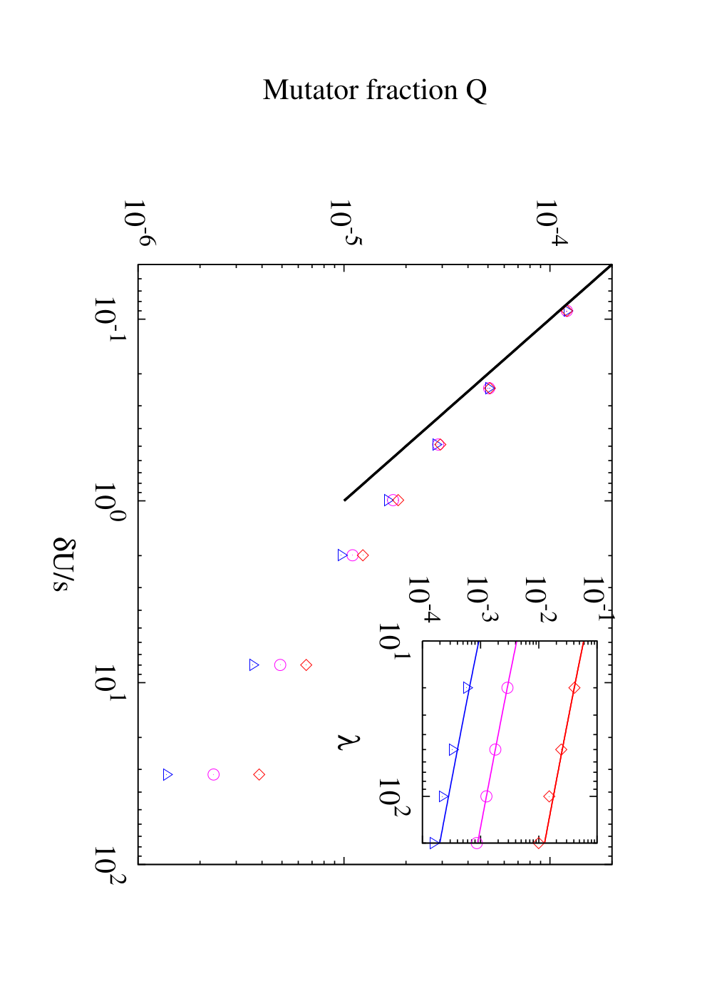
The mutator fraction at mutation-selection balance has been calculated by several authors on non-epistatic fitness landscapes. While Johnson (1999); Desai and Fisher (2011) computed it for a general distribution of fitness effects and small conversion rate , an exact solution was obtained for arbitrary by Nagar and Jain (2009) when all mutations have the same selective effect. In their work, Desai and Fisher (2011) have pointed out that the behavior of the mutator fraction depends on the relative strength of mutational effects () to selective effects (). When selective disadvantage exceeds the mutational effects, the mutations can be treated as effectively lethal (Johnson, 1999; Desai and Fisher, 2011). This is because when (regime I), the most populated nonmutator fitness class in (48) is below unity and therefore the nonmutator population is effectively localised in the fitness class with zero deleterious mutations. As a consequence, mutators which arise due to nonmutators, are also localised in the zero mutation class. Setting all the nonmutator and mutator fractions other than in the zeroth mutational class to zero, (18) immediately leads to (24) which is (unsurprisingly) independent of epistasis. Moreover the result (24) is expected to be insensitive to the distribution of selective effects also (Desai and Fisher, 2011) since both subpopulations are localised in the zero mutation class. However in the opposite limit (regime II), mutator subpopulation is spread over many fitness classes and the simple argument given above underestimates the mutator fraction as can be seen by extrapolating the solution (24) to regime II in Figs. 2-4. An expression for mutator frequency in regime II has been obtained in the absence of epistasis (Johnson, 1999; Nagar and Jain, 2009; Desai and Fisher, 2011) and here we have extended the previous analyses by including it.
Figures 2-4 show that the mutator fraction in regime II decreases monotonically as the epistasis parameter increases. To understand this behavior, we first note that the fitness difference for large approaches zero for and infinity for as increases. Thus the mutators stand a better chance of survival when the fitness interactions are antagonistic than synergistic. For a given , as large selective cost is detrimental for the mutators, the mutator frequency decreases (regime II) to a constant (regime I) as increases (refer Fig. 2). The effect of increasing mutator strength is also to reduce the mutator fraction as shown in Fig. 4. The variation of mutator frequency with the spontaneous mutation rate shown in Fig. 3 however displays an interesting feature: as increases, the mutator frequency decreases monotonically for but for , it decreases in regime I and increases in regime II. At , the mutator fraction decreases to a constant as mutation rate is raised. This behavior may be understood as follows: in regime II in which both subpopulations are spread over the fitness landscape and carry many deleterious mutations, both nonmutators and mutators incur a negligible fitness cost when a mutation occurs for small but due to the unidirectional flux from nonmutators to mutators, the mutator fraction approaches unity as increases (also see Appendix A). This suggests that even if the spontaneous mutation rate of the nonmutator is high, the mutators can still thrive provided the fitness cost increases sufficiently slowly.
On non-epistatic fitness landscapes, the short time dynamics (Johnson, 1999; Desai and Fisher, 2011) until the population reaches a mutation-selection balance and the long term dynamics (Söderberg and Berg, 2011; Lynch, 2011) in which the mutators get fixed due to stochastic fluctuations have been studied. Here we have developed a diffusion theory to find the time to fix mutators in a population of size when the conversion rate is small in the presence of epistatic interactions. Our results given in (39) predict that the fixation time remains roughly constant for small populations and increase exponentially fast beyond a critical population size . Thus in the limit , the time to fix mutators is also infinite which is consistent with the result that an infinitely large population with conversion rate exists in a mixed state. The fixation time depends on the biological parameters through the mutator fraction at mutation-selection balance. In regime I, since the mutator fraction is independent of , this has the direct consequence that the fixation time is also unaffected by (refer Fig. 5) and therefore experiments aiming to detect epistasis using mutators should not operate in regime I. From (24), we find that the crossover population size is approximately for the parameters in Fig. 5 in agreement with the simulation results shown in the inset. The fixation time in regime II depends on the epistasis exponent in a nontrivial manner. As discussed above, the mutator fraction in regime II decreases with increasing and therefore due to (39), it is expected that the time to fix mutators increases and the crossover population size decreases as increases. These expectations are borne out by the simulation results in Fig. 6. We also note that since the mutator fraction in regime II is higher than in regime I, the fixation time in regime II is shorter than that in regime I. Although the diffusion theory developed here using simple arguments captures the essential features of the fixation time, a more sophisticated analysis based on a path-integral formulation may be required for a better quantitative agreement with the numerical results (Neher and Shraiman, 2012).
Evolution of mutation rates
In this article, we studied the dynamics of the evolutionary process by which the mutation rate of a finite asexual population increases from to in time . This population can in turn produce mutators with mutation rate at a rate which take an average time to fix and so on. Thus the mutation rate of the population can keep increasing in a manner similar to Muller’s ratchet (Muller, 1964) in which an asexual population keeps accumulating deleterious mutations. This ratcheting process has been studied recently by Söderberg and Berg (2011) and Lynch (2011) when epistatic interactions are absent and mutator strength is weak (regime I). Here we have focused on the dynamics of the first click of the ratchet for a more general set of parameters.
When epistasis is absent, we can apply the results obtained here for the first click of the ratchet to the succeeding clicks. Assuming that the conversion rate and mutator strength is same for all clicks of the ratchet, the mutation rate at the th click of the ratchet will increase to . Then using (24) and (27) in the expression (39) for fixation time, we find that the time elapsed between th and th click grows as if and otherwise, where . Thus the time between consecutive fixations increases but the rate of increase is slower in regime II than in regime I. Our analytical estimates above are consistent with the numerical results of Söderberg and Berg (2011) who observed that the fixation time increases with mutation rate and mutator strength . Our results (24) and (39) are also in agreement with those of Lynch (2011) who, using a diffusion theory and simulations, showed that the mean time to fixation is roughly constant in and selective effects during the initial clicks characterised by but increases exponentially fast for later clicks. On epistatic fitness landscapes, as the time between successive clicks of the ratchet depends on the fittest class available at the end of a click (Jain, 2008), a quantitative understanding of the successive fixation process requires more work and will be discussed elsewhere. Here we merely speculate that for , every successive fixation event will take longer to occur since the mutator fraction decreases with increasing mutation rate and may result in fitness reduction to an extent that the population may not remain viable. On the other hand, as the mutator fraction at mutation-selection balance increases with mutation rate for , the ratchet is expected to click fast but the population may be able to tolerate the errors as the fitness penalty does not increase commensurately. Interestingly in an experiment on bacterium S. typhimurium measuring the decrease in fitness as deleterious mutations accumulate, the mutation rates was varied up to hundred times more than the wild type and the fitness function of the form (1) was found to be consistent with the epistasis exponent for different mutation rates (Maisnier-Patin et al., 2005). Further experimental and theoretical studies of the mutator dynamics on epistatic fitness landscapes are required to better understand the ratcheting process.
Effect of beneficial mutations
In the discussion so far, we have assumed that the backward conversion rate at which a mutator is created from a nonmutator is zero. This assumption is motivated by experiments on E. coli which indicate that (Ninio, 1991). Here we briefly discuss how a nonzero backward rate affects our main results. An immediate consequence of the nonmutator creation is that the population remains in a mixed state, irrespective of its size. In the inset of Fig. 5, the nonmutator fraction as a function of time is shown when the backward rate is nonzero. We find that the nonmutator frequency is high for about generations after which the mutators take over. However as the nonmutators can be created at a rate , the mutators cease to dominate after generations and the process repeats. In Figs. 5 and 6, the results of our numerical simulations measuring the average time at which the nonmutator fraction becomes zero for the first time is compared with the fixation time for mutators when for a wide range of parameters and we find that the loss time for nonmutators is mildly affected when the mutators are allowed to convert to nonmutators. However the time during which mutators dominate (data not shown) can not be obtained by merely interchanging the nonmutator and mutator labels since the mutators by definition carry a higher mutation rate. A complete analysis of this model is nontrivial and we hope to address it in a future study.
Here we focused on the mutator fixation when the mutations are deleterious but theoretical studies (Andre and Godelle, 2006; Gerrish et al., 2007; Wylie et al., 2009) indicate that the mutators will take over during adaptation also. In this scenario, besides the continual production of mutators and finite population size, an additional factor namely availability of beneficial mutations is at work. As a result, the mutators are likely to get fixed in a time shorter than the one computed here. Indeed our numerical results shown in Fig. 7 for a model in which beneficial mutations can also occur are in agreement with this expectation. In a recent experiment by Raynes et al. (2012), the number of generations for the mutators to take over an adapting population of S. cerevisiae was measured. The fixation time was observed to increase with population size but in very large populations, the mutators were not seen to fix. The latter result is surprising since we have shown here that a finite asexual population will fix mutators even in the absence of beneficial mutations. As the fixation time is large for larger populations, a longer run of the said experiment may shed some light on the dynamics of mutator fixation during adaptation.
Appendix A: Infinite population on sharp peak fitness landscape
When the exponent in (1), we get a sharp peak fitness landscape defined as
| (40) |
The conversion rate at which the transition occurs depends on the nature of the pure mutator state. If the mutator population is in the localised state, (10) holds. But if the mutator population is uniformly distributed with an average population fitness , we have
| (41) |
Moreover, using (40) in (5) and (6), we obtain
| (42) | |||||
| (43) |
On summing over from zero to infinity on both sides of the above equations and using , we get
| (44) |
which shows that the total nonmutator fraction vanishes at both and in accordance with the above discussion and the pure mutator state is the only solution for .
Appendix B: Evaluation of product (22)
The product (22) can be rewritten as
| (45) | |||||
| (46) | |||||
| (47) |
where we have approximated the sum by an integral. The function is nonmonotonic in and has a maximum at given by
| (48) |
This can be seen by considering the ratio which crosses unity at . As the population fraction given by (15) also has a maximum at , the dominant contribution to the sums in (21) comes when the argument . As a result, the upper limit of the integral on the RHS of (47) scales as
| (49) |
if the mutator strength . This allows us to write
| (50) | |||||
| (51) |
Appendix C: Gaussian approximation in regime II
To find the mutator fraction in regime II, we first note that both and have a maximum at given by (48). Using the Stirling’s formula in (15), we approximate the fraction by a Gaussian centred about and obtain
| (52) |
which is normalised to unity for . The product (51) can also be approximated in a similar fashion and we have
| (53) | |||||
| (54) | |||||
| (55) |
For strong mutators, we thus obtain
| (56) |
Note that the width of the above Gaussian approximating the product is about times larger than that of the Gaussian in (52).
Appendix D: Calculation of fixation time (39)
Using the drift coefficient (34) and diffusion coefficient (38) in the expressions (28) and (29), we get
| (57) |
where
| (58) |
and . Thus we have
| (59) |
We first evaluate the integrals in the above equation for by writing where
| (60) | |||||
| (61) |
Since the factor in the inner integral on the RHS of (60) diverges at unity for , the dominant contribution to the integral comes due to this factor:
| (62) | |||||
| (63) |
If , the above integral gives the fixation time to be independent of i.e.
| (64) |
On the other hand, for small and , the integral may be approximated as:
| (65) | |||||
| (66) |
Since , the behavior of the fixation time for is dominated by (64). Thus the diffusion theory predicts that the fixation time for small populations is a constant in . We remark that the -independent behavior of fixation time will not be obtained if instead of (38), Feller diffusion is assumed (see, for e.g., Jain (2008)).
For large populations with , a rough estimate for the fixation time may be obtained using (59). Approximating , we get
| (67) | |||||
| (68) |
Thus for large , the fixation time increases exponentially in .
Acknowledgements
A.N. acknowledges the kind hospitality of JNCASR during his visits.
LITERATURE CITED
- Andre and Godelle (2006) Andre, J.-B. and B. Godelle, 2006. The evolution of mutation rate in finite asexual populations. Genetics 172:611–626.
- Baake and Gabriel (2000) Baake, E. and W. Gabriel, 2000. Pp. 203–264, in D. Stauffer, ed. Annual Reviews of Computational Physics VII. Singapore: World Scientific.
- Baer et al. (2007) Baer, C., M. Miyamoto, and D. Denver, 2007. Mutation rate variation in multicellular eukaryotes: Causes and consequences. Nat. Rev. Genet. 8:619–631.
- Björkholm et al. (2001) Björkholm, B., M. Sjölund, P. Falk, O. Berg, L. Engstrand, and D. Andersson, 2001. Mutation frequency and biological cost of antibiotic resistance in Helicobacter pylori. Proc. Natl. Acad. Sci. USA 98:14607–14612.
- Boe et al. (2000) Boe, L., M. Danielsen, S. Knudsen, J. B. Petersen, J. Maymann, and P. R. Jensen, 2000. The frequency of mutators in populations of Escherichia coli. Mut. Res. 448:47–55.
- Cooper and Lenski (2000) Cooper, V. and R. Lenski, 2000. The population genetics of ecological specialization in evolving Escherichia coli populations. Nature 407:736–739.
- Desai and Fisher (2011) Desai, M. and D. Fisher, 2011. The balance between mutators and nonmutators in asexual populations. Genetics 188:997–1014.
- Drake et al. (1998) Drake, J. W., B. Charlesworth, D. Charlesworth, and J. F. Crow, 1998. Rates of spontaneous mutation. Genetics 148:1667–1686.
- Eigen (1971) Eigen, M., 1971. Selforganization of matter and evolution of biological macromolecules. Naturwissenchaften 58:465 – 523.
- Ewens (1979) Ewens, W., 1979. Mathematical Population Genetics. Springer, Berlin.
- Gentile et al. (2011) Gentile, C., S.-C. Yu, S. Serrano, P. Gerrish, and P. Sniegowski, 2011. Competition between high- and higher-mutating strains of Escherichia coli. Biol. Lett. 7:422–424.
- Gerrish et al. (2007) Gerrish, P. J., A. Colato, A. Perelson, and P. Sniegowski, 2007. Complete genetic linkage can subvert natural selection. Proc. Natl. Acad. Sci. USA 104:6266–6271.
- Gross and Siegel (1981) Gross, M. D. and E. C. Siegel, 1981. Incidence of mutator strains in Esherichia coli and coliforms in nature. Mutat. Res. 91:107–110.
- Haigh (1978) Haigh, J., 1978. The accumulation of deleterious genes in a population - Muller’s ratchet. Theoret. Population Biol. 14:251–267.
- Jain (2008) Jain, K., 2008. Loss of least-loaded class in asexual populations due to drift and epistasis. Genetics 179:2125.
- Jain (2010) ———, 2010. Time to fixation in the presence of recombination. Theo. Pop. Biol. 77:23.
- Jain and Krug (2007) Jain, K. and J. Krug, 2007. Adaptation in simple and complex fitness landscapes. Pp. 299–340, in U. Bastolla, M. Porto, H. Roman, and M. Vendruscolo, eds. Structural Approaches to Sequence Evolution: Molecules, Networks and Populations. Springer, Berlin.
- Jain and Seetharaman (2011) Jain, K. and S. Seetharaman, 2011. Nonlinear deterministic equations in biological evolution. J. Nonlin. Math. Phys. 18:321–338.
- Johnson (1999) Johnson, T., 1999. The approach to mutation — selection balance in an infinite asexual population, and the evolution of mutation rates. Proc. Royal Society B 266:2389.
- Kimura and Maruyama (1966) Kimura, M. and T. Maruyama, 1966. The mutational load with epistatic gene interactions in fitness. Genetics 54:1337–1351.
- Kouyos et al. (2007) Kouyos, R., O. Silander, and S. Bonhoeffer, 2007. Epistasis between deleterious mutations and the evolution of recombination. Trends Ecol. Evol. 22:308–315.
- LeClerc et al. (1996) LeClerc, J., B. Li, W. Payne, and T. Cebula, 1996. High mutation frequencies among Escherichia coli and Salmonella pathogens. Science 274:1208 – 1211.
- Lynch (2011) Lynch, M., 2011. The lower bound to the evolution of mutation rates. Genome Evol. Biol. 3:1107–1118.
- Maisnier-Patin et al. (2005) Maisnier-Patin, S., J. Roth, A. Fredriksson, T. Thomas Nyström, O. Berg, and D. Andersson, 2005. Genomic buffering mitigates the effects of deleterious mutations in bacteria. Nat. Genet. 37:1376 – 1379.
- Mao et al. (1997) Mao, E., L. Lane, J. Lee, and J. Miller, 1997. Proliferation of mutators in a cell population. J. Bacteriol. 179:417–422.
- Matic et al. (1997) Matic, I., M. Radman, F. Taddei, B. Picard, C. Doit, E. Bingen, E. Denamur, and J. Elion, 1997. Highly variable mutation rates in commensal and pathogenic Escherichia coli. Science 277:1833–1834.
- Miller (1996) Miller, J., 1996. Spontaneous mutators in bacteria: Insights into pathways of mutagenesis and repair. Annu. Rev. Microbiol. 50:625–643.
- Muller (1964) Muller, H. J., 1964. The relation of recombination to mutational advance. Mutation Res. 1:2–9.
- Nagar and Jain (2009) Nagar, A. and K. Jain, 2009. Exact phase diagram of quasispecies model with mutation rate modifier. Phys. Rev. Lett. 102:038101.
- Neher and Shraiman (2012) Neher, R. and B. Shraiman, 2009. Fluctuations of fitness distributions and the rate of Muller ratchet. Genetics 191:1283–1293.
- Ninio (1991) Ninio, J., 1991. Transient mutators - a semiquantitative analysis of the influence of translation and transcription errors on mutation rates. Genetics 129:957–962.
- Oliver et al. (2000) Oliver, A., R. Cantón, P. Campo, F. Baquero, and J. Blázquez, 2000. High frequency of hypermutable Pseudomonas aeruginosa in cystic fibrosis lung infection. Science 288:1251–1253.
- Palmer and Lipsitch (2006) Palmer, M. and M. Lipsitch, 2006. The influence of hitchhiking and deleterious mutation upon asexual mutation rates. Genetics 173:461–472.
- Phillips (2008) Phillips, P., 2008. Epistasis: the essential role of gene interactions in the structure and evolution of genetic systems. Nat. Rev. Genet. 9:855–867.
- Raynes et al. (2012) Raynes, Y., M. Gazzara, and P. Sniegowski, 2012. Contrasting dynamics of a mutator allele in asexual populations of differing size. Evolution 66:2329–-2334.
- Richardson et al. (2002) Richardson, A., Z. Yu, T. Popovic, and I. Stojiljkovic, 2002. Mutator clones of Neisseria meningitidis in epidemic serogroup a disease. Proc. Natl. Acad. Sci. USA 99:6103–6107.
- Rosenberg et al. (1998) Rosenberg, S., C. Thulina, and R. Harris, 1998. Transient and heritable mutators in adaptive evolution in the lab and in nature. Genetics 148:1559–1566.
- Shaver et al. (2002) Shaver, A., P. Dombrowski, J. Sweeney, T. Treis, R. Zappala, and P. Sniegowski, 2002. Fitness evolution and the rise of mutator alleles in experimental Escherichia coli populations. Genetics 162:557–566.
- Smith and Haigh (1974) Smith, J. M. and J. Haigh, 1974. Hitchhiking effect of a favourable gene. Genet. Res. 23:23–35.
- Sniegowski et al. (1997) Sniegowski, P. D., P. J. Gerrish, and R. Lenski, 1997. Evolution of high mutation rates in experimental populations of Escherichia coli. Nature 387:703–705.
- Söderberg and Berg (2011) Söderberg, R. and O. Berg, 2011. Kick-starting the ratchet: The fate of mutators in an asexual population. Genetics 187:1129–1137.
- Stephan et al. (1993) Stephan, W., L. Chao, and J. G. Smale, 1993. The advance of Muller ratchet in a haploid asexual population - approximate solutions based on diffusion-theory. Genet. Res. Camb. 61:225–232.
- Stephan and Kim (2002) Stephan, W. and Y. Kim, 2002. Pp. 72–93, in M. Slatkin and M. Veuille, eds. Modern Developments in Theoretical Population Genetics,. Oxford University Press, Oxford.
- Taddei et al. (1997) Taddei, T., M. Radman, J. Maynard-Smith, B. Toupance, P. H. Gouyon, and B. Godelle, 1997. Role of mutator alleles in adaptive evolution. Nature 387:700.
- Tannenbaum and Shakhnovich (2005) Tannenbaum, E. and E. Shakhnovich, 2005. Semiconservative replication in the quasispecies model. Physics of Life Reviews 2:290.
- Tenaillon et al. (1999) Tenaillon, O., B. Toupance, H. Nagard, F. Taddei, and B. Godelle, 1999. Mutators, population size, adaptive landscape and the adaptation of asexual populations of bacteria. Genetics 152:485–493.
- Tröbner and Piechocki (1984) Tröbner, W. and R. Piechocki, 1984. Selection against hypermutability in Escherichia coli during long-term evolution. Mol. Gen. Genet. 198:177–178.
- Visser (2002) Visser, J., 2002. The fate of microbial mutators. Microbiology 148:1247–1252.
- de Visser and Elena (2007) de Visser, J. and S. Elena, 2007. The evolution of sex: empirical insights into the roles of epistasis and drift. Nat. Rev. Genet. 8:139–149.
- Wiehe (1997) Wiehe, T., 1997. Model dependency of error thresholds: the role of fitness functions and contrasts between the finite and infinite sites models. Genet. Res. Camb. 69:127–136.
- Wylie et al. (2009) Wylie, C., C.-M. Ghim, D. Kessler, and H. Levine, 2009. The fixation probability of rare mutators in finite asexual populations. Genetics 181:1595–1612.