跳到论文正文
W Papers独立论文阅读器 arXiv:1205.5948 论文正文 计算阅读时间 · 0%
引用这篇论文根据当前论文元数据生成,正式投稿前建议核对。


License: arXiv.org perpetual non-exclusive license
arXiv:1205.5948v1 [math.AP] 27 May 2012

Effective dynamics of stochastic wave equation with a random dynamical boundary condition Thanks: This work was supported by the National Science Foundation of China (Grants No. 10901115, 10971225 and 11071177) and the Scientific Research Found of Science and Technology Bureau of Sichuan Province (Grant No. 2012JQ0041 and 2010JY0057).

Guanggan Chen Affiliation: College of Mathematics and Software Science, Affiliation: Sichuan Normal University, Chengdu, 610068, China Affiliation: E-mail: chenguanggan@hotmail.com Affiliation: Jinqiao Duan Affiliation: Institute for Pure and Applied Mathematics, Affiliation: University of California, Los Angeles, CA 90095, USA Affiliation: E-mail: jduan@ipam.ucla.edu Affiliation: & Affiliation: Department of Applied Mathematics, Affiliation: Illinois Institute of Technology, Chicago, IL 60616, USA Affiliation: E-mail: duan@iit.edu Affiliation: Jian Zhang Affiliation: College of Mathematics and Software Science, Affiliation: Sichuan Normal University, Chengdu, 610068, China Affiliation: E-mail: zhangjiancdv@sina.com
August 24, 2026

Abstract: This work is devoted to the effective macroscopic dynamics of a weakly damped stochastic nonlinear wave equation with a random dynamical boundary condition. The white noises are taken into account not only in the model equation defined on a domain perforated with small holes, but also in the dynamical boundary condition on the boundaries of the small holes. An effective homogenized, macroscopic model is derived in the sense of probability distribution, which is a new stochastic wave equation on a unified domain, without small holes, with a usual static boundary condition.

Key words: Stochastic partial differential equations; random dynamical boundary condition; effective dynamics; stochastic homogenization; perforated domain.

AMS subject classifications (2010): 60H15, 37L55, 37D10, 37L25, 37H05.

1 Introduction

Nonlinear wave equations, as a class of important mathematical models, describe the propagation of waves in certain systems or media, such as sonic booms, traffic flows, optic devices and quantum fields ([33, 40]). In the deterministic case, they have been studied extensively due to their wide applications in engineering and science (e.g., [20, 22, 31, 34]). On bounded domains or media, the effect of the boundary often needs to be considered. Dirichlet, Neumann and Robin boundary conditions are called static boundary conditions, as they are not involved with time derivatives of the system state variables. On the contrary, dynamic boundary conditions contain time derivatives of the system state variables and arise in many physical problems (see [17, 19, 32]).

In some physical problems, such as wave propagation through the atmosphere or the ocean, due to stochastic force, uncertain parameters, random sources and random boundary conditions, the realistic models take the random fluctuation into account [6, 10, 13]. This leads to stochastic nonlinear wave equations, which have drawn quite attentions recently [7, 10, 11, 15, 23, 24, 26, 43].

In this paper, we are concerned with the effective, macroscopic dynamics of the following “microscopic” weakly damped stochastic nonlinear wave equation with a random dynamical boundary condition on a domain DD perforated with small holes

{ut​tε+utε−△uε+uε−f⁡(uε)=W1˙in​Dε×[0,τ∗),ε2​δt​tε+δtε+ε2​δε=−ε2​utε+ε2​W2˙on​∂Sε×[0,τ∗),uε=0on​∂D×[0,τ∗),δtε=∂uε∂𝐧on​∂Sε×[0,τ∗).\left\{\begin{array}[]{ll}u^{\varepsilon}_{tt}+u^{\varepsilon}_{t}-\bigtriangleup u^{\varepsilon}+u^{\varepsilon}-f(u^{\varepsilon})=\dot{W_{1}}&\quad\hbox{in}\;D^{\varepsilon}\times[0,\tau^{*}),\\ \varepsilon^{2}\delta^{\varepsilon}_{tt}+\delta^{\varepsilon}_{t}+\varepsilon^{2}\delta^{\varepsilon}=-\varepsilon^{2}u^{\varepsilon}_{t}+\varepsilon^{2}\dot{W_{2}}&\quad\hbox{on}\;\partial S^{\varepsilon}\times[0,\tau^{*}),\\ u^{\varepsilon}=0&\quad\hbox{on}\;\partial D\times[0,\tau^{*}),\\ \delta^{\varepsilon}_{t}=\frac{\partial u^{\varepsilon}}{\partial{\bf n}}&\quad\hbox{on}\;\partial S^{\varepsilon}\times[0,\tau^{*}).\end{array}\right. (1.1)

Here ε\varepsilon is a small positive parameter, and the domain DεD^{\varepsilon} is a subset of an open bounded domain DD in ℝ3\mathbb{R}^{3}, obtained by removing SεS^{\varepsilon}, the collection of small holes of size ε\varepsilon, periodically distributed in DD. Also, W1W_{1} and W2W_{2} are two independent Wiener processes. This will be given in details in the next section. The symbol τ∗\tau^{*} denotes a stopping time on (0,+∞)(0,+\infty), and ∂∂𝐧\frac{\partial}{\partial{\bf n}} denotes the unit outer normal derivative on the boundary ∂Sε\partial S^{\varepsilon}. In particular, in this paper we will only concern with the case of the nonlinear term f⁡(uε)=sin⁡uεf(u^{\varepsilon})=\sin u^{\varepsilon} (the Sine-Gordon equation).

The system (1.1), when the white noises, W˙1,W˙2\dot{W}_{1},\dot{W}_{2}, and the parameter ε\varepsilon are absent, arises in the modeling of gas dynamics in an open bounded domain DD, with points on boundary acting like a spring reacting to the excess pressure of the gas (see [16, 25]). In this deterministic case, Beale [3, 4] and Mugnolo [27] established the well-posedness and analyzed some properties of the spectrum in some special cases. Cousin, Frota and Larkin [12] studied the global solvability and asymptotic behavior. Frigeri [16] considered large time dynamical behavior. Furthermore, for the stochastic system (1.1), when the parameter ε\varepsilon are absent, Chen and Zhang [7] investigated the long time behavior of the solutions.

Homogenization plays an important role in understanding multiscale phenomena in material science, climate dynamics, chemistry and biology [8, 36]. For the deterministic system defined on heterogeneous media, there have been some relevant works for heat conduction [28, 29, 35] and for wave propagation [9, 37]. Several authors also considered homogenization problems for the random partial differential equations (PDEs with random coefficients) [21, 30] and for the partial differential equations on randomly heterogeneous domains [5, 41, 42]. However, for the stochastic partial differential equations (PDEs with white noises), especially for the stochastic partial differential equations with random dynamical boundary conditions, due to the effect of both nonlinear dynamical boundary condition and the nonclassical fluctuation of driving white noises, the study of stochastic homogenization problem is still in its infancy (see [38, 39]).

Therefore, in this paper, we are especially interested in the stochastic homogenization problem of Equation (1.1). Our aim is to establish the effective macroscopic equation of Equation (1.1). For this purpose, the key step is to verify the compactness of the solutions in some function space for the deterministic systems. But it does not hold for stochastic Equation (1.1). Therefore, we will instead consider the tightness of the distributions of the solutions, so that the effective macroscopic equation is established in the sense of probability distribution. More precisely, we first analyze the microscopic model Equation (1.1) to establish the well-posedness. Since the energy relation of this stochastic system does not directly imply the a priori estimate of the solutions, we then introduce a pseudo energy argument to infer almost sure boundedness of the solutions. Furthermore, we use the a priori estimate to establish the tightness of distribution of the solutions. Finally, we derive the effective homogenized equation in the sense of probability distribution, which is a new stochastic wave equation on a unified domain without small holes but with a static boundary condition. The solutions of the original model Equation (1.1) converge to those of the effective homogenized equation in probability distribution, as the size of small holes ε\varepsilon diminishes to zero.

This paper is organized as follows. In the next section, we will formulate the basic setup of the homogenization problem. In section 3, we will prove the well-posedness, almost sure boundedness and tightness of distribution of the solutions for the microscopic model Equation (1.1). In section 4, we will derive the effective homogenized equation in probability distribution.

2 Basic setup of the problem

Let the physical medium DD be an open bounded domain in ℝ3\mathbb{R}^{3} with piece-wise smooth boundary ∂D\partial D, and let ε∈(0,1)\varepsilon\in(0,1) be a small real parameter. Denote by Y=[0,l1)×[0,l2)×[0,l3)Y=[0,l_{1})\times[0,l_{2})\times[0,l_{3}) a representative elementary cell in ℝ3\mathbb{R}^{3} and let SS be an open subset of YY with smooth boundary ∂S\partial S such that S⊂YS\subset Y. The elementary cell YY and the small cavity of hole SS inside it are used to model small scale obstacles or heterogeneities in a physical medium DD. Define ε​S={ε​y:y∈S}\varepsilon S=\{\varepsilon y:y\in S\} and Sε,𝐤=𝐤​l+ε​SS_{\varepsilon,{\bf k}}={{\bf k}l+\varepsilon S} with 𝐤​l=(k1​l1,k2​l2,k3​l3){\bf k}l=(k_{1}l_{1},k_{2}l_{2},k_{3}l_{3}) and 𝐤=(k1,k2,k3)∈ℤ3{\bf k}=(k_{1},k_{2},k_{3})\in\mathbb{Z}^{3}. Let SεS^{\varepsilon} be the set of all the holes contained in DD, i.e.,

Sε=⋃{Sε,𝐤|Sε,𝐤¯⊂D,and𝐤∈ℤ3}.S^{\varepsilon}=\bigcup\{S_{\varepsilon,{\bf k}}|\;\overline{S_{\varepsilon,{\bf k}}}\subset D,\hbox{and}\;{\bf k}\in\mathbb{Z}^{3}\}.

Define Dε=D\SεD^{\varepsilon}=D\backslash S^{\varepsilon}. Then DεD^{\varepsilon} is a periodically perforated domain with holes of the same size as period ε\varepsilon. Notice that the holes are assumed to have no intersection with the boundary ∂D\partial D, which implies that ∂Dε=∂D​⋃∂Sε\partial D^{\varepsilon}=\partial D\bigcup\partial S^{\varepsilon}. See Fig.1. This assumption is only needed to avoid technicalities and the results of our paper will remain valid without the assumption [2].

Refer to caption
Figure 1: Geometric setup in ℝ3\mathbb{R}^{3}

In the following, we introduce some other notations. Define Y∗=Y\S¯Y^{*}=Y\backslash\overline{S} and ν=|Y∗||Y|\nu=\frac{|Y^{*}|}{|Y|}, with |Y||Y| and |Y∗||Y^{*}| the Lebesgue measure of YY and Y∗Y^{*} respectively. Denote the indicator function χ\chi as follows

χ⁡(Y)={1,onY∗,0,onS,andχ⁡(D)={1,onDε0,onSε.\chi(Y)=\left\{\begin{array}[]{ll}1,&\quad\hbox{on}\quad Y^{*},\\ 0,&\quad\hbox{on}\quad S,\end{array}\right.\quad\hbox{and}\quad\chi(D)=\left\{\begin{array}[]{ll}1,&\quad\hbox{on}\quad D^{\varepsilon}\\ 0,&\quad\hbox{on}\quad S^{\varepsilon}.\end{array}\right.

We also denote u~\tilde{u} to be the zero extension to the whole domain DD for any function uu defined on the domain DεD^{\varepsilon} as follows

u~={u,onDε,0,onSε.\tilde{u}=\left\{\begin{array}[]{ll}u,&\quad\hbox{on}\quad D^{\varepsilon},\\ 0,&\quad\hbox{on}\quad S^{\varepsilon}.\end{array}\right.

In addition, let the Wiener processes W1​(t)W_{1}(t) and W2​(t)W_{2}(t), defined on a complete probability space (Ω,ℱ,ℙ)(\Omega,\mathcal{F},\mathbb{P}) with the filtration {ℱt}t∈ℝ\{\mathcal{F}_{t}\}_{t\in\mathbb{R}}, be the two-sided in time with values in L2​(D)L^{2}(D). Furthermore, assume that W1​(t)W_{1}(t) and W2​(t)W_{2}(t) are independent and that their covariance operators, Q1Q_{1} and Q2Q_{2}, are symmetric nonnegative operators satisfying T​r​Q1<+∞TrQ_{1}<+\infty and T​r​Q2<+∞TrQ_{2}<+\infty, respectively. Their expansions are given as follows

W1​(t)=∑i=1+∞α1​i​β1​i​ei,withQ1​ei=α1​i​ei,W2​(t)=∑i=1+∞α2​i​β2​i​ei,withQ2​ei=α2​i​ei,\begin{array}[]{l}W_{1}(t)=\sum\limits_{i=1}^{+\infty}\sqrt{\alpha_{1i}}\beta_{1i}e_{i},\quad\hbox{with}\quad Q_{1}e_{i}=\alpha_{1i}e_{i},\\ W_{2}(t)=\sum\limits_{i=1}^{+\infty}\sqrt{\alpha_{2i}}\beta_{2i}e_{i},\quad\hbox{with}\quad Q_{2}e_{i}=\alpha_{2i}e_{i},\end{array}

where {ei}i∈ℕ\{e_{i}\}_{i\in\mathbb{N}} is an orthonormal bases of L2​(D)L^{2}(D), α1​i\alpha_{1i} and α2​i\alpha_{2i} are eigenvalues of Q1,Q2Q_{1},Q_{2} respectively, and {β1​i}i∈ℕ\{\beta_{1i}\}_{i\in\mathbb{N}} and {β2​i}i∈ℕ\{\beta_{2i}\}_{i\in\mathbb{N}} are two sequences of mutually independent (two-sided in time) standard scalar Wiener process on the probability space (Ω,ℱ,ℙ)(\Omega,\mathcal{F},\mathbb{P}).

3 Microscopic Model

Write Equation (1.1) in the Ito^\hat{o} form as follows

{d​uε=vε​d​tin​Dε×[0,τ∗),d​vε=(△uε−uε−vε+sin⁡uε)​d​t+d​W1in​Dε×[0,τ∗),d​δε=θε​d​ton​∂Sε×[0,τ∗),d​θε=(−1ε2​θε−δε−vε)​d​t+d​W2on​∂Sε×[0,τ∗),uε=vε=0,on​∂D×[0,τ∗),δtε=∂uε∂𝐧on​∂Sε×[0,τ∗),\left\{\begin{array}[]{ll}du^{\varepsilon}=v^{\varepsilon}dt&\quad\hbox{in}\;D^{\varepsilon}\times[0,\tau^{*}),\\ dv^{\varepsilon}=(\bigtriangleup u^{\varepsilon}-u^{\varepsilon}-v^{\varepsilon}+\sin u^{\varepsilon})dt+dW_{1}&\quad\hbox{in}\;D^{\varepsilon}\times[0,\tau^{*}),\\ d\delta^{\varepsilon}=\theta^{\varepsilon}dt&\quad\hbox{on}\;\partial S^{\varepsilon}\times[0,\tau^{*}),\\ d\theta^{\varepsilon}=(-\frac{1}{\varepsilon^{2}}\theta^{\varepsilon}-\delta^{\varepsilon}-v^{\varepsilon})dt+dW_{2}&\quad\hbox{on}\;\partial S^{\varepsilon}\times[0,\tau^{*}),\\ u^{\varepsilon}=v^{\varepsilon}=0,&\quad\hbox{on}\;\partial D\times[0,\tau^{*}),\\ \delta^{\varepsilon}_{t}=\frac{\partial u^{\varepsilon}}{\partial{\bf n}}&\quad\hbox{on}\;\partial S^{\varepsilon}\times[0,\tau^{*}),\\ \end{array}\right. (3.1)

We supplement Equation (3.1) with the initial data

uε​(0)=u0,vε​(0)=v0,δε​(0)=δ0,θε​(0)=θ0,u^{\varepsilon}(0)=u_{0},v^{\varepsilon}(0)=v_{0},\delta^{\varepsilon}(0)=\delta_{0},\theta^{\varepsilon}(0)=\theta_{0}, (3.2)

which are ℱ0\mathcal{F}_{0}-measurable.

Now define

Aε=(0I 0 0△−I−I 0 00 0 0I0−I−I−1ε2​I),Fε​(Uε)=(0sin⁡uε00),W=(0W10W2).A^{\varepsilon}=\left(\begin{array}[]{cccc}0&\;I&\;0&\;0\\ \bigtriangleup-I&\;-I&\;0&\;0\\ 0&\;0&\;0&\;I\\ 0&\;-I&\;-I&\;-\frac{1}{\varepsilon^{2}}I\end{array}\right),F^{\varepsilon}(U^{\varepsilon})=\left(\begin{array}[]{l}0\\ \sin u^{\varepsilon}\\ 0\\ 0\end{array}\right),W=\left(\begin{array}[]{l}0\\ W_{1}\\ 0\\ W_{2}\end{array}\right).

Let Uε:=(uε,vε,δε,θε)TU^{\varepsilon}:=(u^{\varepsilon},v^{\varepsilon},\delta^{\varepsilon},\theta^{\varepsilon})^{T} be in the space

ℋε:={Uε∈Hε1​(Dε)×Lε2​(Dε)×L2​(∂Sε)×L2​(∂Sε)|∂uε∂𝐧=θε​on​∂Sε},\mathcal{H}_{\varepsilon}:=\{U^{\varepsilon}\in H_{\varepsilon}^{1}(D^{\varepsilon})\times L_{\varepsilon}^{2}(D^{\varepsilon})\times L^{2}(\partial S^{\varepsilon})\times L^{2}(\partial S^{\varepsilon})|\;\frac{\partial u^{\varepsilon}}{\partial{\bf n}}=\theta^{\varepsilon}\;\hbox{on}\;\partial S^{\varepsilon}\},

with

‖Uε‖ℋε2=‖uε‖Hε1​(Dε)2+‖v‖Lε2​(Dε)2+‖δε‖L2​(∂Sε)2+‖θ‖L2​(∂Sε)2,\|U^{\varepsilon}\|_{\mathcal{H}_{\varepsilon}}^{2}=\|u^{\varepsilon}\|_{H_{\varepsilon}^{1}(D^{\varepsilon})}^{2}+\|v\|_{L_{\varepsilon}^{2}(D^{\varepsilon})}^{2}+\|\delta^{\varepsilon}\|_{L^{2}(\partial S^{\varepsilon})}^{2}+\|\theta\|_{L^{2}(\partial S^{\varepsilon})}^{2},

where Hε1​(Dε)H^{1}_{\varepsilon}(D^{\varepsilon}) and Lε2​(Dε)L^{2}_{\varepsilon}(D^{\varepsilon}) denote the space H1​(Dε)H^{1}(D^{\varepsilon}) and L2​(Dε)L^{2}(D^{\varepsilon}) vanishing on ∂D\partial D, respectively. The superscript “TT” denotes the transpose for the matrix.

Thus Equation (3.1)-(3.2) can be rewritten as

{d​Uε=Aε​Uε​d​t+Fε​(Uε)​d​t+d​W​(t),Uε​(0)=U0ε=(u0,v0,δ0,θ0)T.\left\{\begin{array}[]{l}dU^{\varepsilon}=A^{\varepsilon}U^{\varepsilon}dt+F^{\varepsilon}(U^{\varepsilon})dt+dW(t),\\ U^{\varepsilon}(0)=U_{0}^{\varepsilon}=(u_{0},v_{0},\delta_{0},\theta_{0})^{T}.\end{array}\right. (3.3)

For the Cauchy problem (3.3), it follows from Frigeri [16] that the operator AεA^{\varepsilon} generates a strongly continuous semigroup Sε​(t)={eAε​t}t≥0S^{\varepsilon}(t)=\{e^{A^{\varepsilon}t}\}_{t\geq 0} on ℋε\mathcal{H}_{\varepsilon}. Then the solution of Equation (3.3) can be written in the mild sense

Uε​(t)=Sε​(t)​Uε​(0)+∫0tSε​(t−s)​Fε​(Uε​(s))​𝑑s+∫0tSε​(t−s)​𝑑W​(s).U^{\varepsilon}(t)=S^{\varepsilon}(t)U^{\varepsilon}(0)+\int_{0}^{t}S^{\varepsilon}(t-s)F^{\varepsilon}(U^{\varepsilon}(s))ds+\int_{0}^{t}S^{\varepsilon}(t-s)dW(s). (3.4)

Furthermore, the variational formulation is

∫0τ∗∫Dεuεt​tφdxdt+∫0τ∗∫Dεuεtφdxdt+∫0τ∗∫Dε▽uε▽φdxdt+∫0τ∗∫Dεuεφdxdt−∫0τ∗∫Dεsinuεφdxdt+ε2∫0τ∗∫∂Sεδεt​tφdxdt+ε2∫0τ∗∫∂Sεδεφdxdt=∫0τ∗∫DεW˙1​φ​dx​dt−ε2​∫0τ∗∫∂Sεutε​φ​dx​dt+ε2​∫0τ∗∫∂SεW˙2​φ​dx​dt,\begin{array}[]{ll}&\int_{0}^{\tau^{*}}\int_{D^{\varepsilon}}u^{\varepsilon}_{tt}\varphi dxdt+\int_{0}^{\tau^{*}}\int_{D^{\varepsilon}}u^{\varepsilon}_{t}\varphi dxdt+\int_{0}^{\tau^{*}}\int_{D^{\varepsilon}}\bigtriangledown u^{\varepsilon}\bigtriangledown\varphi dxdt+\int_{0}^{\tau^{*}}\int_{D^{\varepsilon}}u^{\varepsilon}\varphi dxdt\\ &-\int_{0}^{\tau^{*}}\int_{D^{\varepsilon}}\sin u^{\varepsilon}\varphi dxdt+\varepsilon^{2}\int_{0}^{\tau^{*}}\int_{\partial S^{\varepsilon}}\delta^{\varepsilon}_{tt}\varphi dxdt+\varepsilon^{2}\int_{0}^{\tau^{*}}\int_{\partial S^{\varepsilon}}\delta^{\varepsilon}\varphi dxdt\\ =&\int_{0}^{\tau^{*}}\int_{D^{\varepsilon}}\dot{W}_{1}\varphi dxdt-\varepsilon^{2}\int_{0}^{\tau^{*}}\int_{\partial S^{\varepsilon}}u^{\varepsilon}_{t}\varphi dxdt+\varepsilon^{2}\int_{0}^{\tau^{*}}\int_{\partial S^{\varepsilon}}\dot{W}_{2}\varphi dxdt,\end{array} (3.5)

for any φ∈C0∞​([0,τ∗)×Dε)\varphi\in C_{0}^{\infty}([0,\tau^{*})\times D^{\varepsilon}).

Proposition 3.1 (Local well-posedness) Let the initial datum U0εU_{0}^{\varepsilon} be a ℱ0\mathcal{F}_{0}-measurable random variable with value in ℋε\mathcal{H}_{\varepsilon}. Then the Cauchy problem (3.3) has a unique local mild solution Uε​(t)U^{\varepsilon}(t) in C⁡([0,τ∗),ℋε)C([0,\tau^{*}),\mathcal{H}_{\varepsilon}), where τ∗\tau^{*} is a stopping time depending on U0εU_{0}^{\varepsilon} and ω\omega. Moreover, the mild solution Uε​(t)U^{\varepsilon}(t) is also a weak solution in the following sense

⟨Uε​(t),ϕ⟩ℋε=⟨Uε​(0),ϕ⟩ℋε+∫0t⟨Aε​Uε​(s),ϕ⟩ℋε​𝑑s+∫0t⟨Fε​(Uε​(s)),ϕ⟩ℋε​𝑑s+∫0t⟨d​W​(s),ϕ⟩ℋε\langle U^{\varepsilon}(t),\phi\rangle_{\mathcal{H}_{\varepsilon}}=\langle U^{\varepsilon}(0),\phi\rangle_{\mathcal{H}_{\varepsilon}}+\int_{0}^{t}\langle A^{\varepsilon}U^{\varepsilon}(s),\phi\rangle_{\mathcal{H}_{\varepsilon}}ds+\int_{0}^{t}\langle F^{\varepsilon}(U^{\varepsilon}(s)),\phi\rangle_{\mathcal{H}_{\varepsilon}}ds+\int_{0}^{t}\langle dW(s),\phi\rangle_{\mathcal{H}_{\varepsilon}} (3.6)

for any t∈[0,τ∗)t\in[0,\tau^{*}) and ϕ∈ℋε\phi\in\mathcal{H}_{\varepsilon}.

Proof. We first define a cut-off function as follows. For any positive parameter RR, let ηR​(⋅)\eta_{R}(\cdot) be a positive real valued C∞C^{\infty}-function on [0,+∞)[0,+\infty) such that

ηR​(s)={1,for0≤s≤R2,∈(0,1),forR2<s≤R,0,forR<s<+∞.\eta_{R}(s)=\left\{\begin{array}[]{ll}1,&\quad\hbox{for}\quad 0\leq s\leq\frac{R}{2},\\ \in(0,1),&\quad\hbox{for}\quad\frac{R}{2}<s\leq R,\\ 0,&\quad\hbox{for}\quad R<s<+\infty.\end{array}\right.

Then the truncated system of the Cauchy problem (3.3) is defined as follows

{d​Uε=Aε​Uε​d​t+FRε​(Uε)​d​t+d​W​(t),Uε​(0)=U0,\left\{\begin{array}[]{l}dU^{\varepsilon}=A^{\varepsilon}U^{\varepsilon}dt+F^{\varepsilon}_{R}(U^{\varepsilon})dt+dW(t),\\ U^{\varepsilon}(0)=U_{0},\end{array}\right. (3.7)

where FRε(Uε)=(0,ηR(∥Uε∥ℋε2)sinuε,0,0)TF^{\varepsilon}_{R}(U^{\varepsilon})=(0,\eta_{R}(\|U^{\varepsilon}\|_{\mathcal{H}_{\varepsilon}}^{2})\sin u^{\varepsilon},0,0)^{T}.

In the meantime, we easily examine that FRε​(Uε)F^{\varepsilon}_{R}(U^{\varepsilon}) satisfies the sublinear growth and the Lipschitz continuity as in Chen and Zhang [7]. Therefore, according to Theorem 7.4 of Da Prato and Zabczyk [13], the truncated system (3.7) has a unique mild solution URε​(t)U^{\varepsilon}_{R}(t) in ℋε\mathcal{H}_{\varepsilon} for each fixed positive RR.

Define a stopping time

τR:=inf{t:‖Uε‖ℋε2>R2}.\tau_{R}:=\inf\{t:\|U^{\varepsilon}\|_{\mathcal{H}_{\varepsilon}}^{2}>\frac{R}{2}\}. (3.8)

We have Uε​(t)=URε​(t)U^{\varepsilon}(t)=U^{\varepsilon}_{R}(t) as t<τRt<\tau_{R}. Also from Da Prato and Zabczyk [13], the path t→Uε​(t)t\to U^{\varepsilon}(t) is continuous. Let τ∗=limR→+∞τR\tau^{*}=\lim\limits_{R\to+\infty}\tau_{R}. Then Uε​(t)U^{\varepsilon}(t) is the unique local solution of the Cauchy problem (3.3) with lifespan τ∗\tau^{*}. Furthermore, applying the stochastic Fubini theorem, it can be verified that the local mild solution is also the weak solution. The proof is complete. ■\blacksquare

Because the energy relation of this stochastic system does not directly imply the a priori estimate of the solutions, we will introduce a pseudo energy argument (see Chow[11] and Chen and Zhang [7]) to establish the a priori estimate of the solutions for the Cauchy problem (3.3). Furthermore, applying the a priori estimate, we could obtain the global existence and almost sure boundedness of solutions, which further implies the tightness of distribution of solutions.

For a real parameter rr in (0,1)(0,1), we define

vrε=vε+r​uεandθrε=θε+r​δε,v_{r}^{\varepsilon}=v^{\varepsilon}+ru^{\varepsilon}\quad\hbox{and}\quad\theta_{r}^{\varepsilon}=\theta^{\varepsilon}+r\delta^{\varepsilon}, (3.9)

with (uε,vε,δε,θε)T(u^{\varepsilon},v^{\varepsilon},\delta^{\varepsilon},\theta^{\varepsilon})^{T} being the solution of the Cauchy problem (3.1)-(3.2). Then the solution Urε=(uε,vrε,δε,θrε)T∈ℋεU_{r}^{\varepsilon}=(u^{\varepsilon},v_{r}^{\varepsilon},\delta^{\varepsilon},\theta_{r}^{\varepsilon})^{T}\in\mathcal{H}_{\varepsilon} satisfies the following equation

{d​uε=(vrε−r​uε)​d​tin​Dε×[0,τ∗),d​vrε=(△uε−(1−r+r2)​uε−(1−r)​vrε+sin⁡uε)​d​t+d​W1in​Dε×[0,τ∗),d​δε=(θrε−r​δε)​d​ton​∂Sε×[0,τ∗),d​θrε=(−(1ε2−r)​θrε−(1−rε2+r2)​δε−vrε+r​uε)​d​t+d​W2on​∂Sε×[0,τ∗),uε=vrε=0on​∂D×[0,τ∗),δtε=∂uε∂𝐧on​∂Sε×[0,τ∗),uε​(0)=u0,vrε​(0)=v0+r​u0:=vr​0in​Dε,δε​(0)=δ0,θrε​(0)=θ0+r​δ0:=θr​0on​∂Sε.\left\{\begin{array}[]{ll}du^{\varepsilon}=(v_{r}^{\varepsilon}-ru^{\varepsilon})dt&\hbox{in}\;D^{\varepsilon}\times[0,\tau^{*}),\\ dv_{r}^{\varepsilon}=(\bigtriangleup u^{\varepsilon}-(1-r+r^{2})u^{\varepsilon}-(1-r)v_{r}^{\varepsilon}+\sin u^{\varepsilon})dt+dW_{1}&\hbox{in}\;D^{\varepsilon}\times[0,\tau^{*}),\\ d\delta^{\varepsilon}=(\theta_{r}^{\varepsilon}-r\delta^{\varepsilon})dt&\hbox{on}\;\partial S^{\varepsilon}\times[0,\tau^{*}),\\ d\theta_{r}^{\varepsilon}=(-(\frac{1}{\varepsilon^{2}}-r)\theta_{r}^{\varepsilon}-(1-\frac{r}{\varepsilon^{2}}+r^{2})\delta^{\varepsilon}-v_{r}^{\varepsilon}+ru^{\varepsilon})dt+dW_{2}&\hbox{on}\;\partial S^{\varepsilon}\times[0,\tau^{*}),\\ u^{\varepsilon}=v_{r}^{\varepsilon}=0&\hbox{on}\;\partial D\times[0,\tau^{*}),\\ \delta^{\varepsilon}_{t}=\frac{\partial u^{\varepsilon}}{\partial{\bf n}}&\hbox{on}\;\partial S^{\varepsilon}\times[0,\tau^{*}),\\ u^{\varepsilon}(0)=u_{0},v_{r}^{\varepsilon}(0)=v_{0}+ru_{0}:=v_{r0}&\hbox{in}\;D^{\varepsilon},\\ \delta^{\varepsilon}(0)=\delta_{0},\theta_{r}^{\varepsilon}(0)=\theta_{0}+r\delta_{0}:=\theta_{r0}&\hbox{on}\;\partial S^{\varepsilon}.\end{array}\right. (3.10)

Define the pseudo energy functional ℰrε​(t)\mathcal{E}_{r}^{\varepsilon}(t) of the Cauchy problem (3.3) as follows

ℰrε​(t):⁣=‖vrε​(t)‖Lε2​(Dε)2+‖▽uε​(t)‖Lε2​(Dε)2+(1−r+r2)​‖uε​(t)‖Lε2​(Dε)2+‖θrε​(t)‖L2​(∂Sε)2+(1−rε2+r2)​‖δε​(t)‖L2​(∂Sε)2+4​‖cos⁡uε​(t)2‖Lε2​(Dε)2+2​r​⟨uε​(t),δε​(t)⟩L2​(∂Sε).\begin{array}[]{lll}\mathcal{E}_{r}^{\varepsilon}(t)&:=&\|v_{r}^{\varepsilon}(t)\|_{L_{\varepsilon}^{2}(D^{\varepsilon})}^{2}+\|\bigtriangledown u^{\varepsilon}(t)\|_{L_{\varepsilon}^{2}(D^{\varepsilon})}^{2}+(1-r+r^{2})\|u^{\varepsilon}(t)\|_{L_{\varepsilon}^{2}(D^{\varepsilon})}^{2}\\ &&+\|\theta_{r}^{\varepsilon}(t)\|_{L^{2}(\partial S^{\varepsilon})}^{2}+(1-\frac{r}{\varepsilon^{2}}+r^{2})\|\delta^{\varepsilon}(t)\|_{L^{2}(\partial S^{\varepsilon})}^{2}+4\|\cos\frac{u^{\varepsilon}(t)}{2}\|_{L_{\varepsilon}^{2}(D^{\varepsilon})}^{2}\\ &&+2r\langle u^{\varepsilon}(t),\delta^{\varepsilon}(t)\rangle_{L^{2}(\partial S^{\varepsilon})}.\end{array}

Proposition 3.2 Let the initial data Urε​(0)U_{r}^{\varepsilon}(0) be a ℱ0\mathcal{F}_{0}-measurable random variable in L2​(Ω,ℋε)L^{2}(\Omega,\mathcal{H}_{\varepsilon}). Then for any time t∈[0,τ∗)t\in[0,\tau^{*}), we have

ℰrε​(t)=ℰrε(0)−∫0t[2(1−r)∥vrε∥Lε2​(Dε)2+2r∥▽uε∥Lε2​(Dε)2+2r(1−r+r2)∥uε∥Lε2​(Dε)2+2(1ε2−r)∥θrε∥L2​(∂Sε)2+2(1−rε2+r2)r∥δε∥L2​(∂Sε)2]ds+2r∫0t⟨uε,sinuε⟩Lε2​(Dε)ds+4r∫0t⟨uε,θrε⟩L2​(∂Sε)ds−4r2∫0t⟨uε,δε⟩L2​(∂Sε)ds+∫0t⟨2vrε,dW1(s)⟩Lε2​(Dε)+∫0t⟨2θrε,dW2(s)⟩L2​(∂Sε)+t​T​r​Q1+t​T​r​Q2.\begin{array}[]{ll}\mathcal{E}_{r}^{\varepsilon}(t)=&\mathcal{E}_{r}^{\varepsilon}(0)-\int_{0}^{t}[2(1-r)\|v_{r}^{\varepsilon}\|_{L_{\varepsilon}^{2}(D^{\varepsilon})}^{2}+2r\|\bigtriangledown u^{\varepsilon}\|_{L_{\varepsilon}^{2}(D^{\varepsilon})}^{2}+2r(1-r+r^{2})\|u^{\varepsilon}\|_{L_{\varepsilon}^{2}(D^{\varepsilon})}^{2}\\ &\quad\quad\quad\quad+2(\frac{1}{\varepsilon^{2}}-r)\|\theta_{r}^{\varepsilon}\|_{L^{2}(\partial S^{\varepsilon})}^{2}+2(1-\frac{r}{\varepsilon^{2}}+r^{2})r\|\delta^{\varepsilon}\|_{L^{2}(\partial S^{\varepsilon})}^{2}]ds\\ &+2r\int_{0}^{t}\langle u^{\varepsilon},\sin u^{\varepsilon}\rangle_{L_{\varepsilon}^{2}(D^{\varepsilon})}ds+4r\int_{0}^{t}\langle u^{\varepsilon},\theta_{r}^{\varepsilon}\rangle_{L^{2}(\partial S^{\varepsilon})}ds-4r^{2}\int_{0}^{t}\langle u^{\varepsilon},\delta^{\varepsilon}\rangle_{L^{2}(\partial S^{\varepsilon})}ds\\ &+\int_{0}^{t}\langle 2v_{r}^{\varepsilon},dW_{1}(s)\rangle_{L_{\varepsilon}^{2}(D^{\varepsilon})}+\int_{0}^{t}\langle 2\theta_{r}^{\varepsilon},dW_{2}(s)\rangle_{L^{2}(\partial S^{\varepsilon})}\\ &+tTrQ_{1}+tTrQ_{2}.\end{array} (3.11)

Moreover,

𝔼​ℰrε​(t)=𝔼​ℰrε​(0)−∫0t[2(1−r)𝔼∥vrε∥Lε2​(Dε)2+2r𝔼∥▽uε∥Lε2​(Dε)2+2r(1−r+r2)𝔼∥uε∥Lε2​(Dε)2+2(1ε2−r)𝔼∥θrε∥L2​(∂Sε)2+2(1−rε2+r2)r𝔼∥δε∥L2​(∂Sε)2]ds+2r∫0t𝔼⟨uε,sinuε⟩Lε2​(Dε)ds+4r∫0t𝔼⟨uε,θrε⟩L2​(∂Sε)ds−4r2∫0t𝔼⟨uε,δε⟩L2​(∂Sε)ds+tTrQ1+tTrQ2.\begin{array}[]{ll}\mathbb{E}\mathcal{E}_{r}^{\varepsilon}(t)=&\mathbb{E}\mathcal{E}_{r}^{\varepsilon}(0)\\ &-\int_{0}^{t}[2(1-r)\mathbb{E}\|v_{r}^{\varepsilon}\|_{L_{\varepsilon}^{2}(D^{\varepsilon})}^{2}+2r\mathbb{E}\|\bigtriangledown u^{\varepsilon}\|_{L_{\varepsilon}^{2}(D^{\varepsilon})}^{2}+2r(1-r+r^{2})\mathbb{E}\|u^{\varepsilon}\|_{L_{\varepsilon}^{2}(D^{\varepsilon})}^{2}\\ &\quad\quad+2(\frac{1}{\varepsilon^{2}}-r)\mathbb{E}\|\theta_{r}^{\varepsilon}\|_{L^{2}(\partial S^{\varepsilon})}^{2}+2(1-\frac{r}{\varepsilon^{2}}+r^{2})r\mathbb{E}\|\delta^{\varepsilon}\|_{L^{2}(\partial S^{\varepsilon})}^{2}]ds\\ &+2r\int_{0}^{t}\mathbb{E}\langle u^{\varepsilon},\sin u^{\varepsilon}\rangle_{L_{\varepsilon}^{2}(D^{\varepsilon})}ds+4r\int_{0}^{t}\mathbb{E}\langle u^{\varepsilon},\theta_{r}^{\varepsilon}\rangle_{L^{2}(\partial S^{\varepsilon})}ds\\ &-4r^{2}\int_{0}^{t}\mathbb{E}\langle u^{\varepsilon},\delta^{\varepsilon}\rangle_{L^{2}(\partial S^{\varepsilon})}ds+tTrQ_{1}+tTrQ_{2}.\end{array} (3.12)

Proof. First, we examine the second equation of (3.10). Put M⁡(vrε):=∫Dε|vrε|2​𝑑xM(v_{r}^{\varepsilon}):=\int_{D^{\varepsilon}}|v_{r}^{\varepsilon}|^{2}dx. Then from Ito^\hat{o} formula, we deduce that

M⁡(vrε​(t))=M⁡(vrε​(0))+∫0t⟨M′​(vrε),d​W1​(s)⟩Lε2​(Dε)+∫0t12​T​r​[M′′​(vrε)​Q112​(Q112)∗]​𝑑s+∫0t⟨M′(vrε),(△uε−(1−r+r2)uε−(1−r)vrε+sinuε)⟩Lε2​(Dε)ds,\begin{array}[]{ll}M(v_{r}^{\varepsilon}(t))=&M(v_{r}^{\varepsilon}(0))+\int_{0}^{t}\langle M^{\prime}(v_{r}^{\varepsilon}),dW_{1}(s)\rangle_{L_{\varepsilon}^{2}(D^{\varepsilon})}+\int_{0}^{t}\frac{1}{2}Tr[M^{\prime\prime}(v_{r}^{\varepsilon})Q_{1}^{\frac{1}{2}}(Q_{1}^{\frac{1}{2}})^{*}]ds\\ &+\int_{0}^{t}\langle M^{\prime}(v_{r}^{\varepsilon}),(\bigtriangleup u^{\varepsilon}-(1-r+r^{2})u^{\varepsilon}-(1-r)v_{r}^{\varepsilon}+\sin u^{\varepsilon})\rangle_{L_{\varepsilon}^{2}(D^{\varepsilon})}ds,\end{array} (3.13)

with M′​(vrε)=2​vrεM^{\prime}(v_{r}^{\varepsilon})=2v_{r}^{\varepsilon} and M′′​(vrε)=2​φM^{\prime\prime}(v_{r}^{\varepsilon})=2\varphi for any φ\varphi in Lε2​(Dε)L_{\varepsilon}^{2}(D^{\varepsilon}). After some calculations, we get that

⟨M′​(vrε),(△uε−(1−r+r2)​uε−(1−r)​vrε+sin⁡uε)⟩Lε2​(Dε)=−dd​s​[‖▽uε‖Lε2​(Dε)2+(1−r+r2)​‖uε‖Lε2​(Dε)2+4​‖cos⁡uε2‖Lε2​(Dε)2]−[2​r​‖▽uε‖Lε2​(Dε)2+2​r​(1−r+r2)​‖uε‖Lε2​(Dε)2+2​(1−r)​‖vrε‖Lε2​(Dε)2]+2​⟨vrε,∂uε∂𝐧⟩L2​(∂Sε)+2​r​⟨uε,sin⁡uε⟩Lε2​(Dε).\begin{array}[]{ll}&\langle M^{\prime}(v_{r}^{\varepsilon}),(\bigtriangleup u^{\varepsilon}-(1-r+r^{2})u^{\varepsilon}-(1-r)v_{r}^{\varepsilon}+\sin u^{\varepsilon})\rangle_{L_{\varepsilon}^{2}(D^{\varepsilon})}\\ =&-\frac{d}{ds}[\|\bigtriangledown u^{\varepsilon}\|_{L_{\varepsilon}^{2}(D^{\varepsilon})}^{2}+(1-r+r^{2})\|u^{\varepsilon}\|_{L_{\varepsilon}^{2}(D^{\varepsilon})}^{2}+4\|\cos\frac{u^{\varepsilon}}{2}\|_{L_{\varepsilon}^{2}(D^{\varepsilon})}^{2}]\\ &-[2r\|\bigtriangledown u^{\varepsilon}\|_{L_{\varepsilon}^{2}(D^{\varepsilon})}^{2}+2r(1-r+r^{2})\|u^{\varepsilon}\|_{L_{\varepsilon}^{2}(D^{\varepsilon})}^{2}+2(1-r)\|v_{r}^{\varepsilon}\|_{L_{\varepsilon}^{2}(D^{\varepsilon})}^{2}]\\ &+2\langle v_{r}^{\varepsilon},\frac{\partial u^{\varepsilon}}{\partial{\bf n}}\rangle_{L^{2}(\partial S^{\varepsilon})}+2r\langle u^{\varepsilon},\sin u^{\varepsilon}\rangle_{L_{\varepsilon}^{2}(D^{\varepsilon})}.\end{array} (3.14)

It immediately follows from (3.13) and (3.14) that

‖vrε​(t)‖Lε2​(Dε)2+‖▽uε​(t)‖Lε2​(Dε)2+(1−r+r2)​‖uε​(t)‖Lε2​(Dε)2+4​‖cos⁡uε​(t)2‖Lε2​(Dε)2=‖vrε​(0)‖Lε2​(Dε)2+‖▽uε​(0)‖Lε2​(Dε)2+(1−r+r2)​‖uε​(0)‖Lε2​(Dε)2+4​‖cos⁡uε​(0)2‖Lε2​(Dε)2−∫0t[2(1−r)∥vrε∥Lε2​(Dε)2+2r∥▽uε∥Lε2​(Dε)2+2r(1−r+r2)∥uε∥Lε2​(Dε)2]ds+2∫0t⟨vrε,∂uε∂𝐧⟩L2​(∂Sε)ds+2r∫0t⟨uε,sinuε⟩Lε2​(Dε)ds+∫0t⟨2vrε,dW1(s)⟩Lε2​(Dε)+tTrQ1.\begin{array}[]{ll}&\|v_{r}^{\varepsilon}(t)\|_{L_{\varepsilon}^{2}(D^{\varepsilon})}^{2}+\|\bigtriangledown u^{\varepsilon}(t)\|_{L_{\varepsilon}^{2}(D^{\varepsilon})}^{2}+(1-r+r^{2})\|u^{\varepsilon}(t)\|_{L_{\varepsilon}^{2}(D^{\varepsilon})}^{2}+4\|\cos\frac{u^{\varepsilon}(t)}{2}\|_{L_{\varepsilon}^{2}(D^{\varepsilon})}^{2}\\ =&\|v_{r}^{\varepsilon}(0)\|_{L_{\varepsilon}^{2}(D^{\varepsilon})}^{2}+\|\bigtriangledown u^{\varepsilon}(0)\|_{L_{\varepsilon}^{2}(D^{\varepsilon})}^{2}+(1-r+r^{2})\|u^{\varepsilon}(0)\|_{L_{\varepsilon}^{2}(D^{\varepsilon})}^{2}+4\|\cos\frac{u^{\varepsilon}(0)}{2}\|_{L_{\varepsilon}^{2}(D^{\varepsilon})}^{2}\\ &-\int_{0}^{t}[2(1-r)\|v_{r}^{\varepsilon}\|_{L_{\varepsilon}^{2}(D^{\varepsilon})}^{2}+2r\|\bigtriangledown u^{\varepsilon}\|_{L_{\varepsilon}^{2}(D^{\varepsilon})}^{2}+2r(1-r+r^{2})\|u^{\varepsilon}\|_{L_{\varepsilon}^{2}(D^{\varepsilon})}^{2}]ds\\ &+2\int_{0}^{t}\langle v_{r}^{\varepsilon},\frac{\partial u^{\varepsilon}}{\partial{\bf n}}\rangle_{L^{2}(\partial S^{\varepsilon})}ds+2r\int_{0}^{t}\langle u^{\varepsilon},\sin u^{\varepsilon}\rangle_{L_{\varepsilon}^{2}(D^{\varepsilon})}ds\\ &+\int_{0}^{t}\langle 2v_{r}^{\varepsilon},dW_{1}(s)\rangle_{L_{\varepsilon}^{2}(D^{\varepsilon})}+tTrQ_{1}.\end{array} (3.15)

Second, we examine the fourth equation of (3.10) and M⁡(θrε)=∫∂Sε|θrε|2​𝑑xM(\theta_{r}^{\varepsilon})=\int_{\partial S^{\varepsilon}}|\theta_{r}^{\varepsilon}|^{2}dx. Note that

M⁡(θrε​(t))=M⁡(θrε​(0))+∫0t⟨M′​(θrε),d​W2​(s)⟩L2​(∂Sε)+∫0t12​T​r​[M′′​(θrε)​Q212​(Q212)∗]​𝑑s+∫0t⟨M′(θrε),(−(1ε2−r)θrε−(1−rε2+r2)δε−vrε+ruε)⟩L2​(∂Sε)ds,\begin{array}[]{lll}M(\theta_{r}^{\varepsilon}(t))&=&M(\theta_{r}^{\varepsilon}(0))+\int_{0}^{t}\langle M^{\prime}(\theta_{r}^{\varepsilon}),dW_{2}(s)\rangle_{L^{2}(\partial S^{\varepsilon})}+\int_{0}^{t}\frac{1}{2}Tr[M^{\prime\prime}(\theta_{r}^{\varepsilon})Q_{2}^{\frac{1}{2}}(Q_{2}^{\frac{1}{2}})^{*}]ds\\ &&+\int_{0}^{t}\langle M^{\prime}(\theta_{r}^{\varepsilon}),(-(\frac{1}{\varepsilon^{2}}-r)\theta_{r}^{\varepsilon}-(1-\frac{r}{\varepsilon^{2}}+r^{2})\delta^{\varepsilon}-v_{r}^{\varepsilon}+ru^{\varepsilon})\rangle_{L^{2}(\partial S^{\varepsilon})}ds,\end{array} (3.16)

with M′​(θrε)=2​θrεM^{\prime}(\theta_{r}^{\varepsilon})=2\theta_{r}^{\varepsilon} and M′′​(θrε)=2​ϕM^{\prime\prime}(\theta_{r}^{\varepsilon})=2\phi for any ϕ\phi in L2​(∂Sε)L^{2}(\partial S^{\varepsilon}). After some calculations, we conclude that

⟨M′​(θrε),(−(1ε2−r)​θrε−(1−rε2+r2)​δε−vrε+r​uε)⟩L2​(∂Sε)=−(1−rε2+r2)​dd​s​‖δε‖L2​(∂Sε)2−2​(1−rε2+r2)​r​‖δε‖L2​(∂Sε)2−2​(1ε2−r)​‖θrε‖L2​(∂Sε)2−2​⟨∂uε∂𝐧,vrε⟩L2​(∂Sε)−2​r​⟨δε,vrε⟩L2​(∂Sε)+2​r​⟨θrε,uε⟩L2​(∂Sε).\begin{array}[]{ll}&\langle M^{\prime}(\theta_{r}^{\varepsilon}),(-(\frac{1}{\varepsilon^{2}}-r)\theta_{r}^{\varepsilon}-(1-\frac{r}{\varepsilon^{2}}+r^{2})\delta^{\varepsilon}-v_{r}^{\varepsilon}+ru^{\varepsilon})\rangle_{L^{2}(\partial S^{\varepsilon})}\\ =&-(1-\frac{r}{\varepsilon^{2}}+r^{2})\frac{d}{ds}\|\delta^{\varepsilon}\|_{L^{2}(\partial S^{\varepsilon})}^{2}-2(1-\frac{r}{\varepsilon^{2}}+r^{2})r\|\delta^{\varepsilon}\|_{L^{2}(\partial S^{\varepsilon})}^{2}-2(\frac{1}{\varepsilon^{2}}-r)\|\theta_{r}^{\varepsilon}\|_{L^{2}(\partial S^{\varepsilon})}^{2}\\ &-2\langle\frac{\partial u^{\varepsilon}}{\partial{\bf n}},v_{r}^{\varepsilon}\rangle_{L^{2}(\partial S^{\varepsilon})}-2r\langle\delta^{\varepsilon},v_{r}^{\varepsilon}\rangle_{L^{2}(\partial S^{\varepsilon})}+2r\langle\theta_{r}^{\varepsilon},u^{\varepsilon}\rangle_{L^{2}(\partial S^{\varepsilon})}.\end{array} (3.17)

It follows from (3.16) and (3.17) that

‖θrε​(t)‖L2​(∂Sε)2+(1−rε2+r2)​‖δε​(t)‖L2​(∂Sε)2=‖θε​(0)‖L2​(∂Sε)2+(1−rε2+r2)​‖δε​(0)‖L2​(∂Sε)2−∫0t[2(1−rε2+r2)r∥δε∥L2​(∂Sε)2+2(1ε2−r)∥θrε∥L2​(∂Sε)2]ds−2∫0t⟨∂uε∂𝐧,vrε⟩L2​(∂Sε)ds−2r∫0t⟨δε,vrε⟩L2​(∂Sε)ds+2r∫0t⟨θrε,uε⟩L2​(∂Sε)ds+∫0t⟨2θrε,dW2(s)⟩L2​(∂Sε)+tTrQ2.\begin{array}[]{ll}&\|\theta_{r}^{\varepsilon}(t)\|_{L^{2}(\partial S^{\varepsilon})}^{2}+(1-\frac{r}{\varepsilon^{2}}+r^{2})\|\delta^{\varepsilon}(t)\|_{L^{2}(\partial S^{\varepsilon})}^{2}\\ =&\|\theta^{\varepsilon}(0)\|_{L^{2}(\partial S^{\varepsilon})}^{2}+(1-\frac{r}{\varepsilon^{2}}+r^{2})\|\delta^{\varepsilon}(0)\|_{L^{2}(\partial S^{\varepsilon})}^{2}\\ &-\int_{0}^{t}[2(1-\frac{r}{\varepsilon^{2}}+r^{2})r\|\delta^{\varepsilon}\|_{L^{2}(\partial S^{\varepsilon})}^{2}+2(\frac{1}{\varepsilon^{2}}-r)\|\theta_{r}^{\varepsilon}\|_{L^{2}(\partial S^{\varepsilon})}^{2}]ds\\ &-2\int_{0}^{t}\langle\frac{\partial u^{\varepsilon}}{\partial{\bf n}},v_{r}^{\varepsilon}\rangle_{L^{2}(\partial S^{\varepsilon})}ds-2r\int_{0}^{t}\langle\delta^{\varepsilon},v_{r}^{\varepsilon}\rangle_{L^{2}(\partial S^{\varepsilon})}ds+2r\int_{0}^{t}\langle\theta_{r}^{\varepsilon},u^{\varepsilon}\rangle_{L^{2}(\partial S^{\varepsilon})}ds\\ &+\int_{0}^{t}\langle 2\theta_{r}^{\varepsilon},dW_{2}(s)\rangle_{L^{2}(\partial S^{\varepsilon})}+tTrQ_{2}.\end{array} (3.18)

Thus, from (3.15) and (3.18), we have

‖vrε​(t)‖Lε2​(Dε)2+‖▽uε​(t)‖Lε2​(Dε)2+(1−r+r2)​‖uε​(t)‖Lε2​(Dε)2+‖θrε​(t)‖L2​(∂Sε)2+(1−rε2+r2)​‖δε​(t)‖L2​(∂Sε)2+4​‖cos⁡uε​(t)2‖Lε2​(Dε)2=‖vrε​(0)‖Lε2​(Dε)2+‖▽uε​(0)‖Lε2​(Dε)2+(1−r+r2)​‖uε​(0)‖Lε2​(Dε)2+‖θε​(0)‖L2​(∂Sε)2+(1−rε2+r2)​‖δε​(0)‖L2​(∂Sε)2+4​‖cos⁡uε​(0)2‖Lε2​(Dε)2−∫0t[2(1−r)∥vrε∥Lε2​(Dε)2+2r∥▽uε∥Lε2​(Dε)2+2r(1−r+r2)∥uε∥Lε2​(Dε)2+2(1ε2−r)∥θrε∥L2​(∂Sε)2+2(1−rε2+r2)r∥δε∥L2​(∂Sε)2]ds+2r∫0t⟨uε,sinuε⟩Lε2​(Dε)ds−2r∫0t⟨δε,vrε⟩L2​(∂Sε)ds+2r∫0t⟨θrε,uε⟩L2​(∂Sε)ds+∫0t⟨2vrε,dW1(s)⟩Lε2​(Dε)+∫0t⟨2θrε,dW2(s)⟩L2​(∂Sε)+tTrQ1+tTrQ2.\begin{array}[]{ll}&\|v_{r}^{\varepsilon}(t)\|_{L_{\varepsilon}^{2}(D^{\varepsilon})}^{2}+\|\bigtriangledown u^{\varepsilon}(t)\|_{L_{\varepsilon}^{2}(D^{\varepsilon})}^{2}+(1-r+r^{2})\|u^{\varepsilon}(t)\|_{L_{\varepsilon}^{2}(D^{\varepsilon})}^{2}+\|\theta_{r}^{\varepsilon}(t)\|_{L^{2}(\partial S^{\varepsilon})}^{2}\\ &+(1-\frac{r}{\varepsilon^{2}}+r^{2})\|\delta^{\varepsilon}(t)\|_{L^{2}(\partial S^{\varepsilon})}^{2}+4\|\cos\frac{u^{\varepsilon}(t)}{2}\|_{L_{\varepsilon}^{2}(D^{\varepsilon})}^{2}\\ =&\|v_{r}^{\varepsilon}(0)\|_{L_{\varepsilon}^{2}(D^{\varepsilon})}^{2}+\|\bigtriangledown u^{\varepsilon}(0)\|_{L_{\varepsilon}^{2}(D^{\varepsilon})}^{2}+(1-r+r^{2})\|u^{\varepsilon}(0)\|_{L_{\varepsilon}^{2}(D^{\varepsilon})}^{2}+\|\theta^{\varepsilon}(0)\|_{L^{2}(\partial S^{\varepsilon})}^{2}\\ &+(1-\frac{r}{\varepsilon^{2}}+r^{2})\|\delta^{\varepsilon}(0)\|_{L^{2}(\partial S^{\varepsilon})}^{2}+4\|\cos\frac{u^{\varepsilon}(0)}{2}\|_{L_{\varepsilon}^{2}(D^{\varepsilon})}^{2}\\ &-\int_{0}^{t}[2(1-r)\|v_{r}^{\varepsilon}\|_{L_{\varepsilon}^{2}(D^{\varepsilon})}^{2}+2r\|\bigtriangledown u^{\varepsilon}\|_{L_{\varepsilon}^{2}(D^{\varepsilon})}^{2}+2r(1-r+r^{2})\|u^{\varepsilon}\|_{L_{\varepsilon}^{2}(D^{\varepsilon})}^{2}\\ &+2(\frac{1}{\varepsilon^{2}}-r)\|\theta_{r}^{\varepsilon}\|_{L^{2}(\partial S^{\varepsilon})}^{2}+2(1-\frac{r}{\varepsilon^{2}}+r^{2})r\|\delta^{\varepsilon}\|_{L^{2}(\partial S^{\varepsilon})}^{2}]ds\\ &+2r\int_{0}^{t}\langle u^{\varepsilon},\sin u^{\varepsilon}\rangle_{L_{\varepsilon}^{2}(D^{\varepsilon})}ds-2r\int_{0}^{t}\langle\delta^{\varepsilon},v_{r}^{\varepsilon}\rangle_{L^{2}(\partial S^{\varepsilon})}ds+2r\int_{0}^{t}\langle\theta_{r}^{\varepsilon},u^{\varepsilon}\rangle_{L^{2}(\partial S^{\varepsilon})}ds\\ &+\int_{0}^{t}\langle 2v_{r}^{\varepsilon},dW_{1}(s)\rangle_{L_{\varepsilon}^{2}(D^{\varepsilon})}+\int_{0}^{t}\langle 2\theta_{r}^{\varepsilon},dW_{2}(s)\rangle_{L^{2}(\partial S^{\varepsilon})}+tTrQ_{1}+tTrQ_{2}.\end{array} (3.19)

Meanwhile, we note that

2​r​⟨uε​(t),δε​(t)⟩L2​(∂Sε)=2​r​⟨uε​(0),δε​(0)⟩L2​(∂Sε)+2​r​∫0t⟨(uε)s,δε⟩L2​(∂Sε)​𝑑s+2​r​∫0t⟨uε,(δε)s⟩L2​(∂Sε)​𝑑s=2​r​⟨uε​(0),δε​(0)⟩L2​(∂Sε)+2​r​∫0t⟨vε,δε⟩L2​(∂Sε)​𝑑s+2​r​∫0t⟨uε,θε⟩L2​(∂Sε)​𝑑s=2​r​⟨uε​(0),δε​(0)⟩L2​(∂Sε)+2​r​∫0t⟨vrε−r​uε,δε⟩L2​(∂Sε)​𝑑s+2​r​∫0t⟨uε,θrε−r​δε⟩L2​(∂Sε)​𝑑s=2​r​⟨uε​(0),δε​(0)⟩L2​(∂Sε)+2​r​∫0t⟨vrε,δε⟩L2​(∂Sε)​𝑑s+2​r​∫0t⟨uε,θrε⟩L2​(∂Sε)​𝑑s−4r2∫0t⟨uε,δε⟩L2​(∂Sε)ds,\begin{array}[]{ll}&2r\langle u^{\varepsilon}(t),\delta^{\varepsilon}(t)\rangle_{L^{2}(\partial S^{\varepsilon})}\\ =&2r\langle u^{\varepsilon}(0),\delta^{\varepsilon}(0)\rangle_{L^{2}(\partial S^{\varepsilon})}+2r\int_{0}^{t}\langle(u^{\varepsilon})_{s},\delta^{\varepsilon}\rangle_{L^{2}(\partial S^{\varepsilon})}ds+2r\int_{0}^{t}\langle u^{\varepsilon},(\delta^{\varepsilon})_{s}\rangle_{L^{2}(\partial S^{\varepsilon})}ds\\ =&2r\langle u^{\varepsilon}(0),\delta^{\varepsilon}(0)\rangle_{L^{2}(\partial S^{\varepsilon})}+2r\int_{0}^{t}\langle v^{\varepsilon},\delta^{\varepsilon}\rangle_{L^{2}(\partial S^{\varepsilon})}ds+2r\int_{0}^{t}\langle u^{\varepsilon},\theta^{\varepsilon}\rangle_{L^{2}(\partial S^{\varepsilon})}ds\\ =&2r\langle u^{\varepsilon}(0),\delta^{\varepsilon}(0)\rangle_{L^{2}(\partial S^{\varepsilon})}+2r\int_{0}^{t}\langle v_{r}^{\varepsilon}-ru^{\varepsilon},\delta^{\varepsilon}\rangle_{L^{2}(\partial S^{\varepsilon})}ds+2r\int_{0}^{t}\langle u^{\varepsilon},\theta_{r}^{\varepsilon}-r\delta^{\varepsilon}\rangle_{L^{2}(\partial S^{\varepsilon})}ds\\ =&2r\langle u^{\varepsilon}(0),\delta^{\varepsilon}(0)\rangle_{L^{2}(\partial S^{\varepsilon})}+2r\int_{0}^{t}\langle v_{r}^{\varepsilon},\delta^{\varepsilon}\rangle_{L^{2}(\partial S^{\varepsilon})}ds+2r\int_{0}^{t}\langle u^{\varepsilon},\theta_{r}^{\varepsilon}\rangle_{L^{2}(\partial S^{\varepsilon})}ds\\ &-4r^{2}\int_{0}^{t}\langle u^{\varepsilon},\delta^{\varepsilon}\rangle_{L^{2}(\partial S^{\varepsilon})}ds,\end{array}

which implies that

−2r∫0t⟨vrε,δε⟩L2​(∂Sε)ds=−2​r​⟨uε​(t),δε​(t)⟩L2​(∂Sε)+2​r​⟨uε​(0),δε​(0)⟩L2​(∂Sε)+2​r​∫0t⟨uε,θrε⟩L2​(∂Sε)​𝑑s−4r2∫0t⟨uε,δε⟩L2​(∂Sε)ds.\begin{array}[]{ll}&-2r\int_{0}^{t}\langle v_{r}^{\varepsilon},\delta^{\varepsilon}\rangle_{L^{2}(\partial S^{\varepsilon})}ds\\ =&-2r\langle u^{\varepsilon}(t),\delta^{\varepsilon}(t)\rangle_{L^{2}(\partial S^{\varepsilon})}+2r\langle u^{\varepsilon}(0),\delta^{\varepsilon}(0)\rangle_{L^{2}(\partial S^{\varepsilon})}+2r\int_{0}^{t}\langle u^{\varepsilon},\theta_{r}^{\varepsilon}\rangle_{L^{2}(\partial S^{\varepsilon})}ds\\ &-4r^{2}\int_{0}^{t}\langle u^{\varepsilon},\delta^{\varepsilon}\rangle_{L^{2}(\partial S^{\varepsilon})}ds.\end{array} (3.20)

Then it follows from (3.19) and (3.20) that (3.11) and (3.12) hold. ■\blacksquare

Proposition 3.3 Let the initial datum Urε​(0)U_{r}^{\varepsilon}(0) be a ℱ0\mathcal{F}_{0}-measurable random variable in L2​(Ω,ℋε)L^{2}(\Omega,\mathcal{H}_{\varepsilon}). Then for any time t∈[0,τ∗)t\in[0,\tau^{*}), and a sufficient small rr in (0,1)(0,1), there exists a positive constant CC such that

𝔼​‖Urε​(t)‖ℋε2≤C​𝔼​ℰrε​(0)−C​∫0t[𝔼​‖Urε​(s)‖ℋε2]​𝑑s+C⁡[t​T​r​Q1+t​T​r​Q2+t].\mathbb{E}\|U_{r}^{\varepsilon}(t)\|_{\mathcal{H}_{\varepsilon}}^{2}\leq C\mathbb{E}\mathcal{E}_{r}^{\varepsilon}(0)-C\int_{0}^{t}[\mathbb{E}\|U_{r}^{\varepsilon}(s)\|_{\mathcal{H}_{\varepsilon}}^{2}]ds+C[tTrQ_{1}+tTrQ_{2}+t]. (3.21)

Proof. On the one hand, it follows from the Cauchy inequality and the trace inequality that there exists a positive constant CT​I>0C_{TI}>0 (here and hereafter CT​IC_{TI} denotes the positive constant in the trace inequality) such that

0≤r​𝔼​‖uε​(t)‖L2​(∂Sε)2+2​r​𝔼​⟨uε​(t),δε​(t)⟩L2​(∂Sε)+r​𝔼​‖δε​(t)‖L2​(∂Sε)2≤r​CT​I2​𝔼​‖uε​(t)‖Hε1​(Dε)2+2​r​𝔼​⟨uε​(t),δε​(t)⟩L2​(∂Sε)+r​𝔼​‖δε​(t)‖L2​(∂Sε)2,\begin{array}[]{ll}0&\leq r\mathbb{E}\|u^{\varepsilon}(t)\|_{L^{2}(\partial S^{\varepsilon})}^{2}+2r\mathbb{E}\langle u^{\varepsilon}(t),\delta^{\varepsilon}(t)\rangle_{L^{2}(\partial S^{\varepsilon})}+r\mathbb{E}\|\delta^{\varepsilon}(t)\|_{L^{2}(\partial S^{\varepsilon})}^{2}\\ &\leq rC_{TI}^{2}\mathbb{E}\|u^{\varepsilon}(t)\|_{H_{\varepsilon}^{1}(D^{\varepsilon})}^{2}+2r\mathbb{E}\langle u^{\varepsilon}(t),\delta^{\varepsilon}(t)\rangle_{L^{2}(\partial S^{\varepsilon})}+r\mathbb{E}\|\delta^{\varepsilon}(t)\|_{L^{2}(\partial S^{\varepsilon})}^{2},\end{array}

which implies that

𝔼​ℰrε​(t)≥𝔼​‖vrε​(t)‖Lε2​(Dε)2+(1−r​CT​I2)​𝔼​‖▽uε​(t)‖Lε2​(Dε)2+(1−r−r​CT​I2+r2)​𝔼​‖uε​(t)‖Lε2​(Dε)2+𝔼​‖θrε​(t)‖L2​(∂Sε)2+(1−rε2−r+r2)​𝔼​‖δ⁡(t)‖L2​(∂Sε)2.\begin{array}[]{ll}\mathbb{E}\mathcal{E}_{r}^{\varepsilon}(t)\geq&\mathbb{E}\|v_{r}^{\varepsilon}(t)\|_{L_{\varepsilon}^{2}(D^{\varepsilon})}^{2}+(1-rC_{TI}^{2})\mathbb{E}\|\bigtriangledown u^{\varepsilon}(t)\|_{L_{\varepsilon}^{2}(D^{\varepsilon})}^{2}\\ &+(1-r-rC_{TI}^{2}+r^{2})\mathbb{E}\|u^{\varepsilon}(t)\|_{L_{\varepsilon}^{2}(D^{\varepsilon})}^{2}+\mathbb{E}\|\theta_{r}^{\varepsilon}(t)\|_{L^{2}(\partial S^{\varepsilon})}^{2}\\ &+(1-\frac{r}{\varepsilon^{2}}-r+r^{2})\mathbb{E}\|\delta(t)\|_{L^{2}(\partial S^{\varepsilon})}^{2}.\end{array} (3.22)

On the other hand, it follows from the Ho¨\ddot{o}lder inequality, the Young inequality and the trace inequality that

𝔼​⟨uε,θrε⟩L2​(∂Sε)≤𝔼​‖uε‖L2​(∂Sε)⋅𝔼​‖θrε‖L2​(∂Sε)≤r​𝔼​‖uε‖L2​(∂Sε)2+14​r​𝔼​‖θrε‖L2​(∂Sε)2≤r​CT​I2​𝔼​‖uε‖Hε1​(Dε)2+14​r​𝔼​‖θrε‖L2​(∂Sε)2,\begin{array}[]{ll}\mathbb{E}\langle u^{\varepsilon},\theta_{r}^{\varepsilon}\rangle_{L^{2}(\partial S^{\varepsilon})}&\leq\mathbb{E}\|u^{\varepsilon}\|_{L^{2}(\partial S^{\varepsilon})}\cdot\mathbb{E}\|\theta_{r}^{\varepsilon}\|_{L^{2}(\partial S^{\varepsilon})}\\ &\leq r\mathbb{E}\|u^{\varepsilon}\|_{L^{2}(\partial S^{\varepsilon})}^{2}+\frac{1}{4r}\mathbb{E}\|\theta_{r}^{\varepsilon}\|_{L^{2}(\partial S^{\varepsilon})}^{2}\\ &\leq rC_{TI}^{2}\mathbb{E}\|u^{\varepsilon}\|_{H_{\varepsilon}^{1}(D^{\varepsilon})}^{2}+\frac{1}{4r}\mathbb{E}\|\theta_{r}^{\varepsilon}\|_{L^{2}(\partial S^{\varepsilon})}^{2},\end{array}

which implies that

4​r​𝔼​⟨uε,θrε⟩L2​(∂Sε)≤4​r2​CT​I2​𝔼​‖▽uε‖Lε2​(Dε)2+4​r2​CT​I2​𝔼​‖uε‖Lε2​(Dε)2+𝔼​‖θrε‖L2​(∂Sε)2.4r\mathbb{E}\langle u^{\varepsilon},\theta_{r}^{\varepsilon}\rangle_{L^{2}(\partial S^{\varepsilon})}\leq 4r^{2}C_{TI}^{2}\mathbb{E}\|\bigtriangledown u^{\varepsilon}\|_{L_{\varepsilon}^{2}(D^{\varepsilon})}^{2}+4r^{2}C_{TI}^{2}\mathbb{E}\|u^{\varepsilon}\|_{L_{\varepsilon}^{2}(D^{\varepsilon})}^{2}+\mathbb{E}\|\theta_{r}^{\varepsilon}\|_{L^{2}(\partial S^{\varepsilon})}^{2}. (3.23)

At the same time, it follows from the Cauchy inequality and the trace inequality that

−4​r2​𝔼​⟨uε,δε⟩L2​(∂Sε)≤2​r2​𝔼​‖uε‖L2​(∂Sε)2+2​r2​𝔼​‖δε‖L2​(∂Sε)2≤2​r2​CT​I2​𝔼​‖▽uε‖Lε2​(Dε)2+2​r2​CT​I2​𝔼​‖uε‖Lε2​(Dε)2+2​r2​𝔼​‖δε‖L2​(∂Sε)2.\begin{array}[]{ll}-4r^{2}\mathbb{E}\langle u^{\varepsilon},\delta^{\varepsilon}\rangle_{L^{2}(\partial S^{\varepsilon})}&\leq 2r^{2}\mathbb{E}\|u^{\varepsilon}\|_{L^{2}(\partial S^{\varepsilon})}^{2}+2r^{2}\mathbb{E}\|\delta^{\varepsilon}\|_{L^{2}(\partial S^{\varepsilon})}^{2}\\ &\leq 2r^{2}C_{TI}^{2}\mathbb{E}\|\bigtriangledown u^{\varepsilon}\|_{L_{\varepsilon}^{2}(D^{\varepsilon})}^{2}+2r^{2}C_{TI}^{2}\mathbb{E}\|u^{\varepsilon}\|_{L_{\varepsilon}^{2}(D^{\varepsilon})}^{2}+2r^{2}\mathbb{E}\|\delta^{\varepsilon}\|_{L^{2}(\partial S^{\varepsilon})}^{2}.\end{array} (3.24)

Also it follows from the Cauchy inequality that

2​r​𝔼​⟨uε,sin⁡uε⟩Lε2​(Dε)≤r​𝔼​‖uε‖Lε2​(Dε)2+r​𝔼​‖sin⁡uε‖Lε2​(Dε)2≤r​𝔼​‖uε‖Lε2​(Dε)2+C.\begin{array}[]{ll}2r\mathbb{E}\langle u^{\varepsilon},\sin u^{\varepsilon}\rangle_{L_{\varepsilon}^{2}(D^{\varepsilon})}&\leq r\mathbb{E}\|u^{\varepsilon}\|_{L_{\varepsilon}^{2}(D^{\varepsilon})}^{2}+r\mathbb{E}\|\sin u^{\varepsilon}\|_{L_{\varepsilon}^{2}(D^{\varepsilon})}^{2}\\ &\leq r\mathbb{E}\|u^{\varepsilon}\|_{L_{\varepsilon}^{2}(D^{\varepsilon})}^{2}+C.\end{array} (3.25)

Notice that ε∈(0,1)\varepsilon\in(0,1). Then it follows from Proposition 3.2 and (3.23)-(3.25) that

𝔼​ℰrε​(t)≤𝔼ℰrε(0)−∫0t[2(1−r)𝔼∥vε∥Lε2​(Dε)2+2r(1−3rCT​I2)𝔼∥▽uε∥Lε2​(Dε)2+r⁡[1−2​r−6​r​CT​I2+2​r2]​𝔼​‖uε‖Lε2​(Dε)2+(1−2r)𝔼∥θε∥L2​(∂Sε)2+2r(1−r−rε2+r2)𝔼∥δε∥L2​(∂Sε)2]ds+t​T​r​Q1+t​T​r​Q2+C​t.\begin{array}[]{ll}\mathbb{E}\mathcal{E}_{r}^{\varepsilon}(t)\leq&\mathbb{E}\mathcal{E}_{r}^{\varepsilon}(0)-\int_{0}^{t}[2(1-r)\mathbb{E}\|v^{\varepsilon}\|_{L_{\varepsilon}^{2}(D^{\varepsilon})}^{2}+2r(1-3rC_{TI}^{2})\mathbb{E}\|\bigtriangledown u^{\varepsilon}\|_{L_{\varepsilon}^{2}(D^{\varepsilon})}^{2}\\ &+r[1-2r-6rC_{TI}^{2}+2r^{2}]\mathbb{E}\|u^{\varepsilon}\|_{L_{\varepsilon}^{2}(D^{\varepsilon})}^{2}\\ &+(1-2r)\mathbb{E}\|\theta^{\varepsilon}\|_{L^{2}(\partial S^{\varepsilon})}^{2}+2r(1-r-\frac{r}{\varepsilon^{2}}+r^{2})\mathbb{E}\|\delta^{\varepsilon}\|_{L^{2}(\partial S^{\varepsilon})}^{2}]ds\\ &+tTrQ_{1}+tTrQ_{2}+Ct.\end{array} (3.26)

Let rr be sufficient small in (0,1)(0,1) such that

min⁡{1−2​r,1−3​r​CT​I2,1−r−rε2+r2,1−2​r−6​r​CT​I2+2​r2,1−r−r​CT​I2+r2}>0.\min\{1-2r,1-3rC_{TI}^{2},1-r-\frac{r}{\varepsilon^{2}}+r^{2},1-2r-6rC_{TI}^{2}+2r^{2},1-r-rC_{TI}^{2}+r^{2}\}>0. (3.27)

Therefore, from (3.22), (3.26) and (3.27), there exists a positive constant CC such that

𝔼​‖vε​(t)‖Lε2​(Dε)2+𝔼​‖▽uε​(t)‖Lε2​(Dε)2+𝔼​‖uε​(t)‖Lε2​(Dε)2+𝔼​‖θrε​(t)‖L2​(∂Sε)2+𝔼​‖δε​(t)‖L2​(∂Sε)2≤Cℰrε(0)−C∫0t[𝔼∥vε(s)∥Lε2​(Dε)2+𝔼∥▽uε(s)∥Lε2​(Dε)2+𝔼​‖uε​(s)‖Lε2​(Dε)2+𝔼​‖θrε​(s)‖L2​(∂Sε)2+𝔼∥δε(s)∥L2​(∂Sε)2]ds+C[tTrQ1+tTrQ2+t],\begin{array}[]{ll}&\mathbb{E}\|v^{\varepsilon}(t)\|_{L_{\varepsilon}^{2}(D^{\varepsilon})}^{2}+\mathbb{E}\|\bigtriangledown u^{\varepsilon}(t)\|_{L_{\varepsilon}^{2}(D^{\varepsilon})}^{2}+\mathbb{E}\|u^{\varepsilon}(t)\|_{L_{\varepsilon}^{2}(D^{\varepsilon})}^{2}\\ &+\mathbb{E}\|\theta_{r}^{\varepsilon}(t)\|_{L^{2}(\partial S^{\varepsilon})}^{2}+\mathbb{E}\|\delta^{\varepsilon}(t)\|_{L^{2}(\partial S^{\varepsilon})}^{2}\\ \leq&C\mathcal{E}_{r}^{\varepsilon}(0)-C\int_{0}^{t}[\mathbb{E}\|v^{\varepsilon}(s)\|_{L_{\varepsilon}^{2}(D^{\varepsilon})}^{2}+\mathbb{E}\|\bigtriangledown u^{\varepsilon}(s)\|_{L_{\varepsilon}^{2}(D^{\varepsilon})}^{2}\\ &+\mathbb{E}\|u^{\varepsilon}(s)\|_{L_{\varepsilon}^{2}(D^{\varepsilon})}^{2}+\mathbb{E}\|\theta_{r}^{\varepsilon}(s)\|_{L^{2}(\partial S^{\varepsilon})}^{2}\\ &+\mathbb{E}\|\delta^{\varepsilon}(s)\|_{L^{2}(\partial S^{\varepsilon})}^{2}]ds+C[tTrQ_{1}+tTrQ_{2}+t],\end{array}

which implies (3.21). ■\blacksquare

Proposition 3.4 Let the initial datum U0εU^{\varepsilon}_{0} be a ℱ0\mathcal{F}_{0}-measurable random variable in L2​(Ω,ℋε)L^{2}(\Omega,\mathcal{H}_{\varepsilon}). Then the solution Uε​(t)U^{\varepsilon}(t) of the Cauchy problem (3.3) globally exists in ℋε\mathcal{H}_{\varepsilon}, i.e. τ∗=+∞\tau^{*}=+\infty almost surely.

Proof. For any given positive T0T_{0}, consider the case that t<τ∗≤T0t<\tau^{*}\leq T_{0}. For any stopping time τ\tau satisfying τ<τ∗\tau<\tau^{*}, it follows from Proposition 3.3 and the Gronwall inequality that for arbitrary t≤τ∧τRt\leq\tau\wedge\tau_{R},

𝔼​‖Urε​(t)‖ℋε2≤C⁡(T0,T​r​Q1,T​r​Q2,𝔼​ℰrε​(0),𝔼​‖Urε​(0)‖ℋε),\mathbb{E}\|U_{r}^{\varepsilon}(t)\|_{\mathcal{H}_{\varepsilon}}^{2}\leq C(T_{0},TrQ_{1},TrQ_{2},\mathbb{E}\mathcal{E}_{r}^{\varepsilon}(0),\mathbb{E}\|U_{r}^{\varepsilon}(0)\|_{\mathcal{H}_{\varepsilon}}), (3.28)

where τR\tau_{R} is defined as (3.8).

Moreover, we note that from Frigeri [16], for r∈(0,12)r\in(0,\frac{1}{2}), 𝔼​‖Urε‖ℋε2≥12​𝔼​‖Uε‖ℋε2\mathbb{E}\|U_{r}^{\varepsilon}\|_{\mathcal{H}_{\varepsilon}}^{2}\geq\frac{1}{2}\mathbb{E}\|U^{\varepsilon}\|_{\mathcal{H}_{\varepsilon}}^{2}. Then take r∈(0,12)r\in(0,\frac{1}{2}) sufficiently small such that (3.27) holds. Then for arbitrary t≤τ∧τRt\leq\tau\wedge\tau_{R},

𝔼​‖Urε​(t)‖ℋε2≥12​𝔼​‖Uε​(t)‖ℋε2≥C𝔼[∥Uε(t)∥ℋε2⋅χ({τR≤T0})]≥C𝔼[R2⋅χ({τR≤T0})]=C⋅R2ℙ{τR≤T0},\begin{array}[]{ll}\mathbb{E}\|U_{r}^{\varepsilon}(t)\|_{\mathcal{H}_{\varepsilon}}^{2}&\geq\frac{1}{2}\mathbb{E}\|U^{\varepsilon}(t)\|_{\mathcal{H}_{\varepsilon}}^{2}\\ &\geq C\mathbb{E}[\|U^{\varepsilon}(t)\|_{\mathcal{H}_{\varepsilon}}^{2}\cdot\chi(\{\tau_{R}\leq T_{0}\})]\\ &\geq C\mathbb{E}[\frac{R}{2}\cdot\chi(\{\tau_{R}\leq T_{0}\})]\\ &=C\cdot\frac{R}{2}\mathbb{P}\{\tau_{R}\leq T_{0}\},\end{array} (3.29)

where χ\chi is the indicator function.

Therefore, from (3.28) and (3.29), we see that

ℙ{τR≤T0}≤2​C​(T0,T​r​Q1,T​r​Q2,𝔼​ℰrε​(0),𝔼​‖Uε​(0)‖ℋε)C​R,\mathbb{P}\{\tau_{R}\leq T_{0}\}\leq\frac{2C(T_{0},TrQ_{1},TrQ_{2},\mathbb{E}\mathcal{E}_{r}^{\varepsilon}(0),\mathbb{E}\|U^{\varepsilon}(0)\|_{\mathcal{H}_{\varepsilon}})}{CR}, (3.30)

which implies from the Borel-Cantelli lemma that

ℙ{τ∗≤T0}=0,\mathbb{P}\{\tau^{*}\leq T_{0}\}=0, (3.31)

where τ∗=limR→+∞τR\tau^{*}=\lim\limits_{R\to+\infty}\tau_{R}. In other words, we conclude that

ℙ{τ∗=∞}=1.\mathbb{P}\{\tau^{*}=\infty\}=1. (3.32)

Therefore the solution Uε​(t)U^{\varepsilon}(t) of the Cauchy problem (3.3) globally exists almost surely. This completes the proof. ■\blacksquare

Proposition 3.5  Let the initial datum U0εU^{\varepsilon}_{0} be a ℱ0\mathcal{F}_{0}-measurable random variable in L2​(Ω,ℋε)L^{2}(\Omega,\mathcal{H}_{\varepsilon}). Then the global solution Uε​(t)U^{\varepsilon}(t) of the Cauchy problem (3.3) is bounded in ℋε\mathcal{H}_{\varepsilon} almost surely.

Proof. From Proposition 3.4, we know that the solution Uε​(t)U^{\varepsilon}(t) of the Cauchy problem (3.3) globally exists on [0,+∞)[0,+\infty) almost surely. Therefore, it follows from Proposition 3.3 that for arbitrary t∈[0,+∞)t\in[0,+\infty),

dd​t​𝔼​‖Urε​(t)‖ℋε2+C​𝔼​‖Urε​(t)‖ℋε2≤C⁡[T​r​Q1+T​r​Q2+1],\frac{d}{dt}\mathbb{E}\|U_{r}^{\varepsilon}(t)\|_{\mathcal{H}_{\varepsilon}}^{2}+C\mathbb{E}\|U_{r}^{\varepsilon}(t)\|_{\mathcal{H}_{\varepsilon}}^{2}\leq C[TrQ_{1}+TrQ_{2}+1],

which immediately implies from the Gronwall inequality that

𝔼​‖Urε​(t)‖ℋε2≤𝔼​‖Urε​(0)‖ℋε2​e−C​t+[T​r​Q1+T​r​Q2+1]​(1−e−C​t).\mathbb{E}\|U_{r}^{\varepsilon}(t)\|_{\mathcal{H}_{\varepsilon}}^{2}\leq\mathbb{E}\|U_{r}^{\varepsilon}(0)\|_{\mathcal{H}_{\varepsilon}}^{2}e^{-Ct}+[TrQ_{1}+TrQ_{2}+1](1-e^{-Ct}). (3.33)

Note that for r∈(0,12)r\in(0,\frac{1}{2}), 𝔼​‖Urε‖ℋε2≥12​𝔼​‖Uε‖ℋε2\mathbb{E}\|U_{r}^{\varepsilon}\|_{\mathcal{H}_{\varepsilon}}^{2}\geq\frac{1}{2}\mathbb{E}\|U^{\varepsilon}\|_{\mathcal{H}_{\varepsilon}}^{2}. Thus we take r∈(0,12)r\in(0,\frac{1}{2}) sufficiently small such that (3.27) holds. It then follows from (3.33) that Proposition 3.5 holds. ■\blacksquare

Introduce a space

Σε:={Uε∈Hε2​(Dε)×Hε1​(Dε)×H1​(∂Sε)×H1​(∂Sε)|∂uε∂𝐧=θε​on​∂Sε},\Sigma_{\varepsilon}:=\{U^{\varepsilon}\in H_{\varepsilon}^{2}(D^{\varepsilon})\times H_{\varepsilon}^{1}(D^{\varepsilon})\times H^{1}(\partial S^{\varepsilon})\times H^{1}(\partial S^{\varepsilon})|\;\frac{\partial u^{\varepsilon}}{\partial{\bf n}}=\theta^{\varepsilon}\;\hbox{on}\;\partial S^{\varepsilon}\},

where Hε2​(Dε)H^{2}_{\varepsilon}(D^{\varepsilon}) and Hε1​(Dε)H^{1}_{\varepsilon}(D^{\varepsilon}) denote the space H2​(Dε)H^{2}(D^{\varepsilon}) and H1​(Dε)H^{1}(D^{\varepsilon}) vanishing on ∂D\partial D, respectively.

Proposition 3.6  Let the initial datum U0εU^{\varepsilon}_{0} be a ℱ0\mathcal{F}_{0}-measurable random variable in L2​(Ω,Σε)L^{2}(\Omega,\Sigma_{\varepsilon}). Then the global solution Uε​(t)U^{\varepsilon}(t) of the Cauchy problem (3.3) is also bounded in Σε\Sigma_{\varepsilon} almost surely.

The proof of Proposition 3.6 is similar as Proposition 3.2, Proposition 3.3 and Proposition 3.5. It is omitted here.

In the following, for any T>0T>0, we consider the solution (uε,vε)T∈L2​(0,T,Hε1​(Dε)×Lε2​(Dε))(u^{\varepsilon},v^{\varepsilon})^{T}\in L^{2}(0,T;H_{\varepsilon}^{1}(D^{\varepsilon})\times L_{\varepsilon}^{2}(D^{\varepsilon})) of Equation (3.1). Set

𝒳:=H1​(D)×L2​(D),𝒴:=L2​(D)×L2​(D),𝒵:=H−1​(D)×L2​(D).\mathcal{X}:=H^{1}(D)\times L^{2}(D),\quad\mathcal{Y}:=L^{2}(D)\times L^{2}(D),\quad\mathcal{Z}:=H^{-1}(D)\times L^{2}(D).

We investigate the behavior of distribution of (uε,vε)T∈L2​(0,T,Lε2​(Dε)×Lε2​(Dε))(u^{\varepsilon},v^{\varepsilon})^{T}\in L^{2}(0,T;L_{\varepsilon}^{2}(D^{\varepsilon})\times L_{\varepsilon}^{2}(D^{\varepsilon})) as ε→0\varepsilon\to 0, which needs the tightness of distribution (see [14]). Notice that the function space changes with ε\varepsilon, which is a difficulty for obtaining the tightness of distributions. Thus we will treat {ℒ((uε,vε)T))}ε>0\{\mathcal{L}((u^{\varepsilon},v^{\varepsilon})^{T}))\}_{\varepsilon>0} as a collection of distributions on L2​((0,T),𝒴)L^{2}((0,T),\mathcal{Y}) by extending (uε,vε)T(u^{\varepsilon},v^{\varepsilon})^{T} to the whole domain DD, whose distribution is defined as ℒ⁡((u~ε,v~ε)T)​(A)=ℙ⁡{ω:(u~ε​(⋅,⋅,ω),v~ε​(⋅,⋅,ω))T∈A}\mathcal{L}((\tilde{u}^{\varepsilon},\tilde{v}^{\varepsilon})^{T})(A)=\mathbb{P}\{\omega:(\tilde{u}^{\varepsilon}(\cdot,\cdot,\omega),\tilde{v}^{\varepsilon}(\cdot,\cdot,\omega))^{T}\in A\} for the Borel set A∈L2​((0,T),𝒴)A\in L^{2}((0,T),\mathcal{Y}).

Proposition 3.7 (Tightness of distribution)  Let the initial datum U0εU^{\varepsilon}_{0} be a ℱ0\mathcal{F}_{0}-measurable random variable in L2​(Ω,ℋε)L^{2}(\Omega,\mathcal{H}_{\varepsilon}), which is independent of W⁡(t)W(t) with 𝔼​‖U0ε‖ℋε2<∞\mathbb{E}\|U^{\varepsilon}_{0}\|_{\mathcal{H}_{\varepsilon}}^{2}<\infty. Then for any T>0T>0, ℒ⁡((uε,vε)T)\mathcal{L}((u^{\varepsilon},v^{\varepsilon})^{T}), the distribution of (uε,vε)T(u^{\varepsilon},v^{\varepsilon})^{T}, is tight in L2​((0,T),𝒴)​⋂C⁡((0,T),𝒵)L^{2}((0,T),\mathcal{Y})\bigcap C((0,T),\mathcal{Z}).

Proof. Firstly, we claim that (uε,vε)T(u^{\varepsilon},v^{\varepsilon})^{T} is bounded almost surely in

G:=L2​(0,T,𝒳)​⋂(W1,2​(0,T,𝒵)+Wα,4​(0,T,𝒴)),G:=L^{2}(0,T;\mathcal{X})\bigcap(W^{1,2}(0,T;\mathcal{Z})+W^{\alpha,4}(0,T;\mathcal{Y})),

where W1,2​(0,T,𝒵)W^{1,2}(0,T;\mathcal{Z}) is a Banach space endowed with the norm

‖φ‖W1,2​(0,T,𝒵)2=‖φ‖L2​(0,T,𝒵)2+‖d​φd​t‖L2​(0,T,𝒵)2<∞,∀φ∈W1,2​(0,T,𝒵),\|\varphi\|_{W^{1,2}(0,T;\mathcal{Z})}^{2}=\|\varphi\|_{L^{2}(0,T;\mathcal{Z})}^{2}+\|\frac{d\varphi}{dt}\|_{L^{2}(0,T;\mathcal{Z})}^{2}<\infty,\quad\forall\quad\varphi\in W^{1,2}(0,T;\mathcal{Z}),

and Wα,4​(0,T,𝒴)W^{\alpha,4}(0,T;\mathcal{Y}) is another Banach space with α∈(14,12)\alpha\in(\frac{1}{4},\frac{1}{2}) endowed with the norm

‖φ‖Wα,4​(0,T,𝒴)4=‖φ‖L4​(0,T,𝒴)4+∫0T∫0T‖φ⁡(t)−φ⁡(s)‖𝒴4|t−s|1+4​α​𝑑s​𝑑t<∞,∀φ∈Wα,4​(0,T,𝒴).\|\varphi\|_{W^{\alpha,4}(0,T;\mathcal{Y})}^{4}=\|\varphi\|_{L^{4}(0,T;\mathcal{Y})}^{4}+\int_{0}^{T}\int_{0}^{T}\frac{\|\varphi(t)-\varphi(s)\|_{\mathcal{Y}}^{4}}{|t-s|^{1+4\alpha}}dsdt<\infty,\quad\forall\quad\varphi\in W^{\alpha,4}(0,T;\mathcal{Y}).

By Proposition 3.5, we know that (uε,vε)T(u^{\varepsilon},v^{\varepsilon})^{T} is bounded in L2​(0,T,𝒳)L^{2}(0,T;\mathcal{X}) almost surely. Therefore, in the following, we only need to prove that (uε,vε)T(u^{\varepsilon},v^{\varepsilon})^{T} is bounded in W1,2​(0,T,𝒵)+Wα,4​(0,T,𝒴)W^{1,2}(0,T;\mathcal{Z})+W^{\alpha,4}(0,T;\mathcal{Y}) almost surely.

Denote by PP the projection operator from UεU^{\varepsilon} to (uε,vε)T(u^{\varepsilon},v^{\varepsilon})^{T}, i.e., P​Uε=(uε,vε)TPU^{\varepsilon}=(u^{\varepsilon},v^{\varepsilon})^{T}. Write Equation (3.3) as

Uε​(t)=Uε​(0)+∫0tAε​Uε​(τ)​𝑑τ+∫0tFε​(Uε​(τ))​𝑑τ+∫0td​W​(τ).U^{\varepsilon}(t)=U^{\varepsilon}(0)+\int_{0}^{t}A^{\varepsilon}U^{\varepsilon}(\tau)d\tau+\int_{0}^{t}F^{\varepsilon}(U^{\varepsilon}(\tau))d\tau+\int_{0}^{t}dW(\tau).

Then

P​Uε​(t)=P​Uε​(0)+∫0t[P​Aε​Uε​(τ)+P​Fε​(Uε​(τ))]​𝑑τ+∫0tP​𝑑W​(τ).PU^{\varepsilon}(t)=PU^{\varepsilon}(0)+\int_{0}^{t}[PA^{\varepsilon}U^{\varepsilon}(\tau)+PF^{\varepsilon}(U^{\varepsilon}(\tau))]d\tau+\int_{0}^{t}PdW(\tau). (3.34)

Denote

I1:=∫0t[P​Aε​Uε​(τ)+P​Fε​(Uε​(τ))]​𝑑τ,I_{1}:=\int_{0}^{t}[PA^{\varepsilon}U^{\varepsilon}(\tau)+PF^{\varepsilon}(U^{\varepsilon}(\tau))]d\tau, (3.35)

and

I2:=∫0tP​𝑑W​(τ).I_{2}:=\int_{0}^{t}PdW(\tau). (3.36)

For I1I_{1}, it follows from Proposition 3.5 and Proposition 3.6 that

𝔼​‖I1‖L2​(0,T,𝒵)2=𝔼​∫0T‖I1​(τ)‖𝒵2​𝑑τ=𝔼​∫0T‖∫0τ[P​Aε​Uε​(s)+P​Fε​(Uε​(s))]​𝑑s‖𝒵2​𝑑τ≤𝔼​∫0T[‖∫0τvε​(s)​𝑑s‖H−1​(D)2+‖∫0τ[△uε​(s)−uε​(s)−vε​(s)+sin⁡uε​(s)]​𝑑s‖L2​(D)2]​𝑑τ≤𝔼∫0T[∫0τ∥vε(s)∥L2​(D)2ds+∫0τ[∥△uε(s)∥L2​(D)2+∥uε(s)∥L2​(D)2+∥vε(s)∥L2​(D)2+∥uε(s)∥L2​(D)2]ds]dτ≤CT,\begin{array}[]{ll}&\mathbb{E}\|I_{1}\|_{L^{2}(0,T;\mathcal{Z})}^{2}\\ =&\mathbb{E}\int_{0}^{T}\|I_{1}(\tau)\|_{\mathcal{Z}}^{2}d\tau\\ =&\mathbb{E}\int_{0}^{T}\|\int_{0}^{\tau}[PA^{\varepsilon}U^{\varepsilon}(s)+PF^{\varepsilon}(U^{\varepsilon}(s))]ds\|_{\mathcal{Z}}^{2}d\tau\\ \leq&\mathbb{E}\int_{0}^{T}[\|\int_{0}^{\tau}v^{\varepsilon}(s)ds\|_{H^{-1}(D)}^{2}+\|\int_{0}^{\tau}[\bigtriangleup u^{\varepsilon}(s)-u^{\varepsilon}(s)-v^{\varepsilon}(s)+\sin u^{\varepsilon}(s)]ds\|_{L^{2}(D)}^{2}]d\tau\\ \leq&\mathbb{E}\int_{0}^{T}[\int_{0}^{\tau}\|v^{\varepsilon}(s)\|_{L^{2}(D)}^{2}ds+\int_{0}^{\tau}[\|\bigtriangleup u^{\varepsilon}(s)\|_{L^{2}(D)}^{2}+\|u^{\varepsilon}(s)\|_{L^{2}(D)}^{2}\\ &+\|v^{\varepsilon}(s)\|_{L^{2}(D)}^{2}+\|u^{\varepsilon}(s)\|_{L^{2}(D)}^{2}]ds]d\tau\\ \leq&C_{T},\end{array} (3.37)

and

𝔼​‖d​I1d​t‖L2​(0,T,𝒵)2=𝔼​∫0T‖d​I1d​τ‖𝒵2​𝑑τ=𝔼​∫0T‖P​Aε​Uε​(τ)+P​Fε​(Uε​(τ))‖𝒵2​𝑑τ≤𝔼​∫0T[‖vε​(τ)‖H−1​(D)2+‖△uε​(τ)−uε​(τ)−vε​(τ)+sin⁡uε​(τ)‖L2​(D)2]​𝑑τ≤𝔼∫0T[∥vε(τ)∥L2​(D)2+∥△uε(τ)∥L2​(D)2+∥uε(τ)∥L2​(D)2+∥vε(τ)∥L2​(D)2+∥uε(τ)∥L2​(D)2]dτ≤CT.\begin{array}[]{ll}&\mathbb{E}\|\frac{dI_{1}}{dt}\|_{L^{2}(0,T;\mathcal{Z})}^{2}\\ =&\mathbb{E}\int_{0}^{T}\|\frac{dI_{1}}{d\tau}\|_{\mathcal{Z}}^{2}d\tau\\ =&\mathbb{E}\int_{0}^{T}\|PA^{\varepsilon}U^{\varepsilon}(\tau)+PF^{\varepsilon}(U^{\varepsilon}(\tau))\|_{\mathcal{Z}}^{2}d\tau\\ \leq&\mathbb{E}\int_{0}^{T}[\|v^{\varepsilon}(\tau)\|_{H^{-1}(D)}^{2}+\|\bigtriangleup u^{\varepsilon}(\tau)-u^{\varepsilon}(\tau)-v^{\varepsilon}(\tau)+\sin u^{\varepsilon}(\tau)\|_{L^{2}(D)}^{2}]d\tau\\ \leq&\mathbb{E}\int_{0}^{T}[\|v^{\varepsilon}(\tau)\|_{L^{2}(D)}^{2}+\|\bigtriangleup u^{\varepsilon}(\tau)\|_{L^{2}(D)}^{2}+\|u^{\varepsilon}(\tau)\|_{L^{2}(D)}^{2}\\ &+\|v^{\varepsilon}(\tau)\|_{L^{2}(D)}^{2}+\|u^{\varepsilon}(\tau)\|_{L^{2}(D)}^{2}]d\tau\\ \leq&C_{T}.\end{array} (3.38)

Here and hereafter, CTC_{T} denotes various positive constants depending on the given T>0T>0. Then combining (3.37) and (3.38), we deduce that

𝔼​‖I1‖W1,2​(0,T,𝒵)2=𝔼​‖I1‖L2​(0,T,𝒵)2+𝔼​‖d​I1d​t‖L2​(0,T,𝒵)2≤CT.\mathbb{E}\|I_{1}\|_{W^{1,2}(0,T;\mathcal{Z})}^{2}=\mathbb{E}\|I_{1}\|_{L^{2}(0,T;\mathcal{Z})}^{2}+\mathbb{E}\|\frac{dI_{1}}{dt}\|_{L^{2}(0,T;\mathcal{Z})}^{2}\leq C_{T}. (3.39)

Now we consider I2I_{2}. Put Mε​(s,t)=∫std​W​(τ)M^{\varepsilon}(s,t)=\int_{s}^{t}dW(\tau). Then using the Burkholder-Davis-Gundy inequality and the Ho¨\ddot{o}lder inequality, we have

𝔼​‖P​Mε​(s,t)‖𝒴4=𝔼​‖∫stP​dW​(τ)‖𝒴4=𝔼​‖∫std​W1​(τ)‖L2​(D)4≤C​𝔼​(∫stT​r​Q1​dτ)2≤C​𝔼​(∫st12​dτ⋅∫st(T​r​Q1)2​dτ)≤C​(t−s)2.\begin{array}[]{ll}\mathbb{E}\|PM^{\varepsilon}(s,t)\|_{\mathcal{Y}}^{4}&=\mathbb{E}\|\int_{s}^{t}PdW(\tau)\|_{\mathcal{Y}}^{4}\\ &=\mathbb{E}\|\int_{s}^{t}dW_{1}(\tau)\|_{L^{2}(D)}^{4}\\ &\leq C\mathbb{E}(\int_{s}^{t}TrQ_{1}d\tau)^{2}\\ &\leq C\mathbb{E}(\int_{s}^{t}1^{2}d\tau\cdot\int_{s}^{t}(TrQ_{1})^{2}d\tau)\\ &\leq C(t-s)^{2}.\end{array} (3.40)

Thus, it follows from (3.40) that

𝔼​‖I2‖L4​(0,T,𝒴)4=𝔼​∫0T‖I2‖𝒴4​𝑑t=𝔼​∫0T‖∫0tP​𝑑W​(τ)‖𝒴4​𝑑t=𝔼​∫0T‖P​Mε​(0,t)‖𝒴4​𝑑t≤∫0TC​(t−0)2​𝑑t≤CT.\begin{array}[]{ll}\mathbb{E}\|I_{2}\|_{L^{4}(0,T;\mathcal{Y})}^{4}&=\mathbb{E}\int_{0}^{T}\|I_{2}\|_{\mathcal{Y}}^{4}dt\\ &=\mathbb{E}\int_{0}^{T}\|\int_{0}^{t}PdW(\tau)\|_{\mathcal{Y}}^{4}dt\\ &=\mathbb{E}\int_{0}^{T}\|PM^{\varepsilon}(0,t)\|_{\mathcal{Y}}^{4}dt\\ &\leq\int_{0}^{T}C(t-0)^{2}dt\\ &\leq C_{T}.\end{array} (3.41)

Also, for α∈(14,12)\alpha\in(\frac{1}{4},\frac{1}{2}), by (3.40), we have

𝔼​∫0T∫0T‖I2​(t)−I2​(s)‖𝒴4|t−s|1+4​α​𝑑s​𝑑t=𝔼​∫0T∫0T‖P​Mε​(0,t)−P​Mε​(0,s)‖𝒴4|t−s|1+4​α​𝑑s​𝑑t=𝔼​∫0T∫0T‖P​Mε​(s,t)‖𝒴4|t−s|1+4​α​𝑑s​𝑑t≤∫0T∫0TC​(t−s)2(t−s)1+4​α​𝑑s​𝑑t≤C​∫0T∫0T(t−s)1−4​α​𝑑s​𝑑t≤CT.\begin{array}[]{ll}\mathbb{E}\int_{0}^{T}\int_{0}^{T}\frac{\|I_{2}(t)-I_{2}(s)\|_{\mathcal{Y}}^{4}}{|t-s|^{1+4\alpha}}dsdt&=\mathbb{E}\int_{0}^{T}\int_{0}^{T}\frac{\|PM^{\varepsilon}(0,t)-PM^{\varepsilon}(0,s)\|_{\mathcal{Y}}^{4}}{|t-s|^{1+4\alpha}}dsdt\\ &=\mathbb{E}\int_{0}^{T}\int_{0}^{T}\frac{\|PM^{\varepsilon}(s,t)\|_{\mathcal{Y}}^{4}}{|t-s|^{1+4\alpha}}dsdt\\ &\leq\int_{0}^{T}\int_{0}^{T}\frac{C(t-s)^{2}}{(t-s)^{1+4\alpha}}dsdt\\ &\leq C\int_{0}^{T}\int_{0}^{T}(t-s)^{1-4\alpha}dsdt\\ &\leq C_{T}.\end{array} (3.42)

Therefore, it follows from (3.41) and (3.42) that for arbitrary α∈(14,12)\alpha\in(\frac{1}{4},\frac{1}{2}),

𝔼​‖I2‖Wα,4​(0,T,𝒴)4=𝔼​‖I2‖L4​(0,T,𝒴)4+𝔼​∫0T∫0T‖I2​(t)−I2​(s)‖𝒴4|t−s|1+4​α​𝑑s​𝑑t<CT.\mathbb{E}\|I_{2}\|_{W^{\alpha,4}(0,T;\mathcal{Y})}^{4}=\mathbb{E}\|I_{2}\|_{L^{4}(0,T;\mathcal{Y})}^{4}+\mathbb{E}\int_{0}^{T}\int_{0}^{T}\frac{\|I_{2}(t)-I_{2}(s)\|_{\mathcal{Y}}^{4}}{|t-s|^{1+4\alpha}}dsdt<C_{T}. (3.43)

Immediately from (3.34)-(3.36), (3.39)and (3.43), we obtain that (uε,vε)T(u^{\varepsilon},v^{\varepsilon})^{T} is bounded in W1,2​(0,T,𝒵)+Wα,4​(0,T,𝒴)W^{1,2}(0,T;\mathcal{Z})+W^{\alpha,4}(0,T;\mathcal{Y}) almost surely, which completes the verification of the claim that (uε,vε)T(u^{\varepsilon},v^{\varepsilon})^{T} is bounded almost surely in G=L2​(0,T,𝒳)​⋂(W1,2​(0,T,𝒵)+Wα,4​(0,T,𝒴))G=L^{2}(0,T;\mathcal{X})\bigcap(W^{1,2}(0,T;\mathcal{Z})+W^{\alpha,4}(0,T;\mathcal{Y})).

By the Chebyshev inequality, we see that for any ρ>0\rho>0, there exists a bounded set Kρ⊂GK_{\rho}\subset G such that ℙ{(uε,vε)T∈Kρ}>1−ρ\mathbb{P}\{(u^{\varepsilon},v^{\varepsilon})^{T}\in K_{\rho}\}>1-\rho. Moreover, notice that

L2​(0,T,𝒳)​⋂W1,2​(0,T,𝒵)⊂L2​(0,T,𝒴)​⋂C⁡(0,T,𝒵),L^{2}(0,T;\mathcal{X)}\bigcap W^{1,2}(0,T;\mathcal{Z})\subset L^{2}(0,T;\mathcal{Y})\bigcap C(0,T;\mathcal{Z}),

and for α∈(14,12)\alpha\in(\frac{1}{4},\frac{1}{2}),

L2​(0,T,𝒳)​⋂Wα,4​(0,T,𝒴)⊂L2​(0,T,𝒴)​⋂C⁡(0,T,𝒵).L^{2}(0,T;\mathcal{X})\bigcap W^{\alpha,4}(0,T;\mathcal{Y})\subset L^{2}(0,T;\mathcal{Y})\bigcap C(0,T;\mathcal{Z}).

We conclude that KρK_{\rho} is compact in L2​(0,T,𝒴)​⋂C⁡(0,T,𝒵)L^{2}(0,T;\mathcal{Y})\bigcap C(0,T;\mathcal{Z}). Thus ℒ⁡((uε,vε)T)\mathcal{L}((u^{\varepsilon},v^{\varepsilon})^{T}) is tight in L2​(0,T,𝒴)​⋂C⁡(0,T,𝒵)L^{2}(0,T;\mathcal{Y})\bigcap C(0,T;\mathcal{Z}). ■\blacksquare

4 Effective Model

In this section, we will use the two-scale method to derive the effective homogenized equation of Equation (1.1), in the sense of probability distribution. The solutions of the microscopic model Equation (1.1) converge to those of the effective homogenized equation in probability distribution, as the size of small holes ε\varepsilon diminishes to zero. The main result is as follows.

Theorem 4.1 (Homogenized model) Let (uε,δε)T(u^{\varepsilon},\delta^{\varepsilon})^{T} be the solution of Equation (1.1). Then for any T>0T>0, the distribution ℒ⁡(u~ε)\mathcal{L}(\tilde{u}^{\varepsilon}) converges weakly to μ\mu in L2​(0,T,L2​(D))L^{2}(0,T;L^{2}(D)) as ε→0\varepsilon\to 0, with μ\mu being the distribution of the solution VV of the following homogenizied equation

{Vt​t(t,x)+Vt(t,x)−ν−1divx𝒜∗(▽xV(t,x))+V(t,x)−sin(V(t,x))=νW˙1,onDV⁡(t,x)=0,on∂DV(0,x)=u0ν,Vt(0,x)=v0ν,onD,\left\{\begin{array}[]{l}V_{tt}(t,x)+V_{t}(t,x)-\nu^{-1}div_{x}\mathcal{A}^{*}(\bigtriangledown_{x}V(t,x))+V(t,x)-\sin(V(t,x))=\nu\dot{W}_{1},\quad\hbox{on}\quad D\\ V(t,x)=0,\quad\hbox{on}\quad\partial D\\ V(0,x)=\frac{u_{0}}{\nu},\quad V_{t}(0,x)=\frac{v_{0}}{\nu},\quad\hbox{on}\quad D,\end{array}\right. (4.1)

where the effective matrix 𝒜∗=(Ai​j∗)\mathcal{A}^{*}=(A_{ij}^{*}) given by (4.21), u0u_{0} and v0v_{0} are the initial data supplemented in Equation (3.2), and the constant ν=|Y∗||Y|\nu=\frac{|Y^{*}|}{|Y|} with |Y||Y| and |Y∗||Y^{*}| the Lebesgue measure of YY and Y∗Y^{*} respectively.

In the following, we will prove Theorem 4.1. We first provide some preliminaries. We will denote by Cp​e​r∞​(Y)C_{per}^{\infty}(Y) the space of infinitely differentiable functions in ℝ3\mathbb{R}^{3} that are periodic in YY. We also denote Lp​e​r2​(Y)L_{per}^{2}(Y) or Hp​e​r1​(Y)H_{per}^{1}(Y) the completion of Cp​e​r∞​(Y)C_{per}^{\infty}(Y) in the usual norm of L2​(Y)L^{2}(Y) or H1​(Y)H^{1}(Y), respectively. In addition, we denote DT=[0,T]×DD_{T}=[0,T]\times D.

Definition 4.1[1] A sequence of functions uε​(t,x)u^{\varepsilon}(t,x) in L2​(DT)L^{2}(D_{T}) is called to be two-scale convergent to a limit u⁡(t,x,y)∈L2​(DT×Y)u(t,x,y)\in L^{2}(D_{T}\times Y), if for any function φ⁡(x,y)∈C0∞​(DT,Cp​e​r∞)\varphi(x,y)\in C_{0}^{\infty}(D_{T},C_{per}^{\infty}),

limε→0∫DTuε​(t,x)​φ​(t,x,xε)​𝑑x​𝑑t=1|Y|​∫DT∫Yu⁡(t,x,y)​φ​(t,x,y)​𝑑y​𝑑x​𝑑t,\lim\limits_{\varepsilon\to 0}\int_{D_{T}}u^{\varepsilon}(t,x)\varphi(t,x,\frac{x}{\varepsilon})dxdt=\frac{1}{|Y|}\int_{D_{T}}\int_{Y}u(t,x,y)\varphi(t,x,y)dydxdt,

which is denoted by uε→2−suu^{\varepsilon}\xlongrightarrow{2-s}u.

Lemma 4.1[1] Let uεu^{\varepsilon} be a bounded sequence in L2​(DT)L^{2}(D_{T}). Then there exists a function u∈L2​(DT×Y)u\in L^{2}(D_{T}\times Y) and a subsequence uεk→0u_{\varepsilon_{k}}\to 0 as k→∞k\to\infty such that uεk→2−suu_{\varepsilon_{k}}\xlongrightarrow{2-s}u.

Lemma 4.2[1] If uε→2−suu^{\varepsilon}\xlongrightarrow{2-s}u, then uε⇀u¯​(t,x)=1|Y|​∫Yu⁡(t,x,y)​𝑑yu^{\varepsilon}\rightharpoonup\overline{u}(t,x)=\frac{1}{|Y|}\int_{Y}u(t,x,y)dy.

Lemma 4.3[1] Let vεv^{\varepsilon} be a sequence in L2​(DT)L^{2}(D_{T}) that two-scale converges to a limit v⁡(x,y)∈L2​(DT×Y)v(x,y)\in L^{2}(D_{T}\times Y). Further assume that

limε→0∫DT|vε​(t,x)|2​𝑑x​𝑑t=1|Y|​∫DT∫Y|v⁡(t,x,y)|2​𝑑y​𝑑x​𝑑t.\lim\limits_{\varepsilon\to 0}\int_{D_{T}}|v^{\varepsilon}(t,x)|^{2}dxdt=\frac{1}{|Y|}\int_{D_{T}}\int_{Y}|v(t,x,y)|^{2}dydxdt.

Then for any sequence uε∈L2​(DT)u^{\varepsilon}\in L^{2}(D_{T}), which two-scale converges to a limit u∈L2​(DT×Y)u\in L^{2}(D_{T}\times Y), we have

uε​vε⇀1|Y|​∫Yu⁡(⋅,⋅,y)​v​(⋅,⋅,y)​𝑑y,as​ε→0​in​L2​(DT).u^{\varepsilon}v^{\varepsilon}\rightharpoonup\frac{1}{|Y|}\int_{Y}u(\cdot,\cdot,y)v(\cdot,\cdot,y)dy,\;\hbox{as}\;\varepsilon\to 0\;\hbox{in}\;L^{2}(D_{T}).

Lemma 4.4[1] Let uεu^{\varepsilon} be a sequence of functions defined on [0,T]×Dε[0,T]\times D^{\varepsilon} which is bounded in L2​(0,T,Hε1​(Dε))L^{2}(0,T;H_{\varepsilon}^{1}(D^{\varepsilon})). There exists u⁡(t,x)∈H01​(DT)u(t,x)\in H_{0}^{1}(D_{T}), u1​(t,x,y)∈L2​(DT,Hp​e​r1​(Y))u_{1}(t,x,y)\in L^{2}(D_{T};H_{per}^{1}(Y)) and a subsequence uεku^{\varepsilon_{k}} with εk→0\varepsilon_{k}\to 0 as k→∞k\to\infty, such that

u~εk​(t,x)→2−sχ⁡(Y)​u​(t,x),k→∞,\tilde{u}^{\varepsilon_{k}}(t,x)\xlongrightarrow{2-s}\chi(Y)u(t,x),\quad k\to\infty,

and

▽xuεk~→2−sχ(Y)[▽xu(t,x)+▽yu1(t,x,y)],k→∞,\widetilde{\bigtriangledown_{x}u^{\varepsilon_{k}}}\xlongrightarrow{2-s}\chi(Y)[\bigtriangledown_{x}u(t,x)+\bigtriangledown_{y}u_{1}(t,x,y)],\quad k\to\infty,

where χ⁡(Y)\chi(Y) is the indicator function as defined in Section 2.

For h∈H−1/2(∂S)h\in H^{-1/2}(\partial S) and YY-periodic, define λh:=1|Y|​∫∂Sh⁡(x)​𝑑x\lambda_{h}:=\frac{1}{|Y|}\int_{\partial S}h(x)dx. Also, for h∈L2​(∂S)h\in L^{2}(\partial S) and YY-periodic, define λhε∈H−1​(D)\lambda_{h}^{\varepsilon}\in H^{-1}(D) as ⟨λhε,φ⟩H−1,H01=ε​∫∂Sεh⁡(xε)​φ​(x)​𝑑x\langle\lambda_{h}^{\varepsilon},\varphi\rangle_{H^{-1},H_{0}^{1}}=\varepsilon\int_{\partial S^{\varepsilon}}h(\frac{x}{\varepsilon})\varphi(x)dx with any φ∈H01​(D)\varphi\in H_{0}^{1}(D).

Lemma 4.5[39] Let φε\varphi^{\varepsilon} be a sequence in H01​(D)H_{0}^{1}(D) such that φε⇀φ\varphi^{\varepsilon}\rightharpoonup\varphi in H01​(D)H_{0}^{1}(D) as ε→0\varepsilon\to 0. Then

⟨λhε,φε|Dε⟩⟶λh​∫Dφ​𝑑x,asε→0.\langle\lambda_{h}^{\varepsilon},\varphi^{\varepsilon}|_{D^{\varepsilon}}\rangle\longrightarrow\lambda_{h}\int_{D}\varphi dx,\quad\hbox{as}\quad\varepsilon\to 0.

Lemma 4.6 (Prohorov Theorem)[13] Suppose ℳ\mathcal{M} is a separable Banach space. The set of probability measures {ℒ⁡(Xn)}n\{\mathcal{L}(X_{n})\}_{n} on (ℳ,ℬ⁡(ℳ))(\mathcal{M},\mathcal{B}(\mathcal{M})) is relatively compact if and only if {Xn}\{X_{n}\} is tight.

Lemma 4.7 (Skorohod Theorem)[13] For an arbitrary sequence of Probability measures {μn}\{\mu_{n}\} on (ℳ,ℬ⁡(ℳ))(\mathcal{M},\mathcal{B}(\mathcal{M})) weakly converges to probability measures μ\mu, there exists a probability space (Ω,ℱ,ℙ)(\Omega,\mathcal{F},\mathbb{P}) and random variables, XX, X1X_{1}, X2X_{2}, ⋯\cdots, XnX_{n}, ⋯\cdots such that XnX_{n} distributes as μn\mu_{n} and XX distributes as μ\mu and limn→∞Xn=X\lim\limits_{n\to\infty}X_{n}=X, ℙ\mathbb{P}-a.s.

Proof of Theorem 4.1.

Let (uε,δε)T(u^{\varepsilon},\delta^{\varepsilon})^{T} be the solution of Equation (1.1). On the one hand, as in [39], by the proof of Proposition 3.7, for any ρ>0\rho>0, there is a bounded set Kρ⊂GK_{\rho}\subset G which is compact in L2​(0,T,𝒴)L^{2}(0,T;\mathcal{Y}) such that ℙ{(u~ε,v~ε)T∈Kρ}>1−ρ\mathbb{P}\{(\tilde{u}^{\varepsilon},\tilde{v}^{\varepsilon})^{T}\in K_{\rho}\}>1-\rho. According to Lemma 4.6 and Lemma 4.7, we know that for any sequence {εj}j=1j=∞\{\varepsilon_{j}\}_{j=1}^{j=\infty} with εj→0\varepsilon_{j}\to 0 as j→∞j\to\infty, there exists a subsequence {εj⁡(k)}k=1k=∞\{\varepsilon_{j(k)}\}_{k=1}^{k=\infty}, random variables {(u~∗εj⁡(k),v~∗εj⁡(k))T}⊂L2​(0,T,Lε2​(Dε)×Lε2​(Dε))\{(\tilde{u}^{\varepsilon_{j(k)}}_{*},\tilde{v}^{\varepsilon_{j(k)}}_{*})^{T}\}\subset L^{2}(0,T;L_{\varepsilon}^{2}(D^{\varepsilon})\times L_{\varepsilon}^{2}(D^{\varepsilon})) and (u∗,v∗)T∈L2​(0,T,𝒴)(u_{*},v_{*})^{T}\in L^{2}(0,T;\mathcal{Y}) defined on a new probability space (Ω∗,ℱ∗,ℙ∗)(\Omega_{*},\mathcal{F}_{*},\mathbb{P}_{*}), such that for almost all ω∈Ω∗\omega\in\Omega_{*},

ℒ⁡((u~∗εj⁡(k),v~∗εj⁡(k))T)=ℒ⁡((u~εj⁡(k),v~εj⁡(k))T),\mathcal{L}((\tilde{u}^{\varepsilon_{j(k)}}_{*},\tilde{v}^{\varepsilon_{j(k)}}_{*})^{T})=\mathcal{L}((\tilde{u}^{\varepsilon_{j(k)}},\tilde{v}^{\varepsilon_{j(k)}})^{T}),

and

(u~∗εj⁡(k),v~∗εj⁡(k))T⟶(u∗,v∗)TinL2​(0,T,𝒴)ask→∞.(\tilde{u}^{\varepsilon_{j(k)}}_{*},\tilde{v}^{\varepsilon_{j(k)}}_{*})^{T}\longrightarrow(u_{*},v_{*})^{T}\quad\hbox{in}\quad L^{2}(0,T;\mathcal{Y})\quad\hbox{as}\quad k\to\infty. (4.2)

In the meantime, (u~∗εj⁡(k),v~∗εj⁡(k))T(\tilde{u}^{\varepsilon_{j(k)}}_{*},\tilde{v}^{\varepsilon_{j(k)}}_{*})^{T} solves

{d​P​Uε=P​Aε​Uε​d​t+P​Fε​(Uε)​d​t+P​d​W​(t),P​Uε​(0)=P​U0,\left\{\begin{array}[]{l}dPU^{\varepsilon}=PA^{\varepsilon}U^{\varepsilon}dt+PF^{\varepsilon}(U^{\varepsilon})dt+PdW(t),\\ PU^{\varepsilon}(0)=PU_{0},\end{array}\right.

with WW being replaced by a Wiener process W∗W_{*}, defined on the probability space (Ω∗,ℱ∗,ℙ∗)(\Omega_{*},\mathcal{F}_{*},\mathbb{P}_{*}) but with the same distributions as WW. Here PP is the projection operator from UεU^{\varepsilon} to (uε,vε)T(u^{\varepsilon},v^{\varepsilon})^{T} as defined in the proof of Proposition 3.7.

On the other hand, for uεu^{\varepsilon} in the set KρK_{\rho}, it follows from Lemma 4.1 and Lemma 4.4 that there exist u⁡(t,x)∈H01​(DT)u(t,x)\in H_{0}^{1}(D_{T}) and u1​(t,x,y)∈L2​(DT,Hp​e​r1​(Y))u_{1}(t,x,y)\in L^{2}(D_{T},H^{1}_{per}(Y)) such that

u~εk​(t,x)→2−sχ⁡(Y)​u​(t,x),k→∞,\tilde{u}^{\varepsilon_{k}}(t,x)\xlongrightarrow{2-s}\chi(Y)u(t,x),\quad k\to\infty, (4.3)

and

▽xuεk~→2−sχ(Y)[▽xu(t,x)+▽yu1(t,x,y)],k→∞.\widetilde{\bigtriangledown_{x}u^{\varepsilon_{k}}}\xlongrightarrow{2-s}\chi(Y)[\bigtriangledown_{x}u(t,x)+\bigtriangledown_{y}u_{1}(t,x,y)],\quad k\to\infty. (4.4)

Furthermore, from Lemma 4.2, it follows that

u~εk​(t,x)⇀1|Y|​∫Yχ⁡(Y)​u​(t,x)​𝑑y=1|Y|​∫Yχ⁡(Y)​𝑑y⋅u⁡(t,x)=ν​u​(t,x),inL2​(DT),\tilde{u}^{\varepsilon_{k}}(t,x)\rightharpoonup\frac{1}{|Y|}\int_{Y}\chi(Y)u(t,x)dy=\frac{1}{|Y|}\int_{Y}\chi(Y)dy\cdot u(t,x)=\nu u(t,x),\quad\hbox{in}\quad L^{2}(D_{T}),

which from the compactness of KρK_{\rho} immediately implies that

u~εk​(t,x)⟶ν​u​(t,x),inL2​(DT).\tilde{u}^{\varepsilon_{k}}(t,x)\longrightarrow\nu u(t,x),\quad\hbox{in}\quad L^{2}(D_{T}). (4.5)

Then combining the relationship of uεu^{\varepsilon} and vεv^{\varepsilon}, (4.2) and (4.5), we have

u∗=ν​uandv∗=ν​ut.u_{*}=\nu u\quad\hbox{and}\quad v_{*}=\nu u_{t}. (4.6)

Now, in the probability space (Ω,ℱ,ℙ)(\Omega,\mathcal{F},\mathbb{P}), we put Ωρ={ω∈Ω:u~ε​(ω)∈Kρ}\Omega_{\rho}=\{\omega\in\Omega:\tilde{u}^{\varepsilon}(\omega)\in K_{\rho}\}, ℱρ={F​⋂Ωρ:F∈ℱ}\mathcal{F}_{\rho}=\{F\bigcap\Omega_{\rho}:F\in\mathcal{F}\}, and ℙρ​(F)=ℙ⁡(F​⋂Ωρ)ℙ⁡(Ωρ)\mathbb{P}_{\rho}(F)=\frac{\mathbb{P}(F\bigcap\Omega_{\rho})}{\mathbb{P}(\Omega_{\rho})}, for F∈ℱρF\in\mathcal{F}_{\rho}. Then (Ωρ,ℱρ,ℙρ)(\Omega_{\rho},\mathcal{F}_{\rho},\mathbb{P}_{\rho}) forms a new probability space, whose expectation operator is denoted by 𝔼ρ\mathbb{E}_{\rho}. In the following, we will work in the probability space (Ωρ,ℱρ,ℙρ)(\Omega_{\rho},\mathcal{F}_{\rho},\mathbb{P}_{\rho}) in stead of (Ω,ℱ,ℙ)(\Omega,\mathcal{F},\mathbb{P}).

In Equation (3.5), we choose the test function φ\varphi as φε​(t,x)=ϕ⁡(t,x)+ε​Φ​(t,x,xε)\varphi^{\varepsilon}(t,x)=\phi(t,x)+\varepsilon\Phi(t,x,\frac{x}{\varepsilon}) with ϕ⁡(t,x)∈C0∞​(DT)\phi(t,x)\in C_{0}^{\infty}(D_{T}) and Φ⁡(t,x,y)∈C0∞​(DT,Cp​e​r∞​(Y))\Phi(t,x,y)\in C_{0}^{\infty}(D_{T};C_{per}^{\infty}(Y)). Also, we notice that (4.5) and χ⁡(Dε)⇀ν\chi(D^{\varepsilon})\rightharpoonup\nu in L∞​(D)L^{\infty}(D). Then we have

∫0T∫Dεut​tε​φε​𝑑x​𝑑t=∫0T∫Dεut​tε​[ϕ⁡(t,x)+ε​Φ​(t,x,xε)]​𝑑x​𝑑t=−∫0T∫Dε[uεtϕt(t,x)+εuεtΦt(t,x,xε)]dxdt=∫0T∫Dε[uε​ϕt​t​(t,x)+ε​uε​Φt​t​(t,x,xε)]​𝑑x​𝑑t=∫0T∫D[u~ε​ϕt​t​(t,x)+ε​u~ε​Φt​t​(t,x,xε)]​𝑑x​𝑑t→∫0T∫Dν​u​(t,x)​ϕt​t​(t,x)​𝑑x​𝑑t=∫0T∫Dν​ut​t​(t,x)​ϕ​(t,x)​dx​dt,asε→0,\begin{array}[]{lll}\int_{0}^{T}\int_{D^{\varepsilon}}u^{\varepsilon}_{tt}\varphi^{\varepsilon}dxdt&=&\int_{0}^{T}\int_{D^{\varepsilon}}u^{\varepsilon}_{tt}[\phi(t,x)+\varepsilon\Phi(t,x,\frac{x}{\varepsilon})]dxdt\\ &=&-\int_{0}^{T}\int_{D^{\varepsilon}}[u^{\varepsilon}_{t}\phi_{t}(t,x)+\varepsilon u^{\varepsilon}_{t}\Phi_{t}(t,x,\frac{x}{\varepsilon})]dxdt\\ &=&\int_{0}^{T}\int_{D^{\varepsilon}}[u^{\varepsilon}\phi_{tt}(t,x)+\varepsilon u^{\varepsilon}\Phi_{tt}(t,x,\frac{x}{\varepsilon})]dxdt\\ &=&\int_{0}^{T}\int_{D}[\tilde{u}^{\varepsilon}\phi_{tt}(t,x)+\varepsilon\tilde{u}^{\varepsilon}\Phi_{tt}(t,x,\frac{x}{\varepsilon})]dxdt\\ &\to&\int_{0}^{T}\int_{D}\nu u(t,x)\phi_{tt}(t,x)dxdt\\ &=&\int_{0}^{T}\int_{D}\nu u_{tt}(t,x)\phi(t,x)dxdt,\quad\hbox{as}\quad\varepsilon\to 0,\end{array} (4.7)
∫0T∫Dεutε​φε​𝑑x​𝑑t=∫0T∫Dεutε​[ϕ⁡(t,x)+ε​Φ​(t,x,xε)]​𝑑x​𝑑t=−∫0T∫Dε[uεϕt(t,x)+εuεΦt(t,x,xε)]dxdt=−∫0T∫D[u~εϕt(t,x)+εu~εΦt(t,x,xε)]dxdt→−∫0T∫Dνu(t,x)ϕt(t,x)dxdt=∫0T∫Dν​ut​(t,x)​ϕ​(t,x)​dx​dt,asε→0,\begin{array}[]{lll}\int_{0}^{T}\int_{D^{\varepsilon}}u^{\varepsilon}_{t}\varphi^{\varepsilon}dxdt&=&\int_{0}^{T}\int_{D^{\varepsilon}}u^{\varepsilon}_{t}[\phi(t,x)+\varepsilon\Phi(t,x,\frac{x}{\varepsilon})]dxdt\\ &=&-\int_{0}^{T}\int_{D^{\varepsilon}}[u^{\varepsilon}\phi_{t}(t,x)+\varepsilon u^{\varepsilon}\Phi_{t}(t,x,\frac{x}{\varepsilon})]dxdt\\ &=&-\int_{0}^{T}\int_{D}[\tilde{u}^{\varepsilon}\phi_{t}(t,x)+\varepsilon\tilde{u}^{\varepsilon}\Phi_{t}(t,x,\frac{x}{\varepsilon})]dxdt\\ &\to&-\int_{0}^{T}\int_{D}\nu u(t,x)\phi_{t}(t,x)dxdt\\ &=&\int_{0}^{T}\int_{D}\nu u_{t}(t,x)\phi(t,x)dxdt,\quad\hbox{as}\quad\varepsilon\to 0,\end{array} (4.8)

and

∫0T∫Dεuε​φε​𝑑x​𝑑t=∫0T∫Dεuε​[ϕ⁡(t,x)+ε​Φ​(t,x,xε)]​𝑑x​𝑑t=∫0T∫D[u~ε​ϕ​(t,x)+ε​u~ε​Φ​(t,x,xε)]​𝑑x​𝑑t→∫0T∫Dν​u​(t,x)​ϕ​(t,x)​dx​dt,asε→0.\begin{array}[]{lll}\int_{0}^{T}\int_{D^{\varepsilon}}u^{\varepsilon}\varphi^{\varepsilon}dxdt&=&\int_{0}^{T}\int_{D^{\varepsilon}}u^{\varepsilon}[\phi(t,x)+\varepsilon\Phi(t,x,\frac{x}{\varepsilon})]dxdt\\ &=&\int_{0}^{T}\int_{D}[\tilde{u}^{\varepsilon}\phi(t,x)+\varepsilon\tilde{u}^{\varepsilon}\Phi(t,x,\frac{x}{\varepsilon})]dxdt\\ &\to&\int_{0}^{T}\int_{D}\nu u(t,x)\phi(t,x)dxdt,\quad\hbox{as}\quad\varepsilon\to 0.\end{array} (4.9)

For φε\varphi^{\varepsilon}, we have

▽xφε=▽xϕ(t,x)+ε▽xΦ(t,x,xε)=▽xϕ(t,x)+▽yΦ(t,x,y)→2−s▽xϕ(t,x)+▽yΦ(t,x,y),asε→0,\begin{array}[]{lcl}\bigtriangledown_{x}\varphi^{\varepsilon}&=&\bigtriangledown_{x}\phi(t,x)+\varepsilon\bigtriangledown_{x}\Phi(t,x,\frac{x}{\varepsilon})\\ &=&\bigtriangledown_{x}\phi(t,x)+\bigtriangledown_{y}\Phi(t,x,y)\\ &\xlongrightarrow{2-s}&\bigtriangledown_{x}\phi(t,x)+\bigtriangledown_{y}\Phi(t,x,y),\quad\hbox{as}\quad\varepsilon\to 0,\end{array} (4.10)

and

limε→0∫DT|▽xφε|2dxdt=limε→0∫DT|▽xϕ(t,x)+ε▽xΦ(t,x,xε)|2dxdt=1|Y|∫DT∫Y|▽xϕ(t,x)+▽yΦ(t,x,y)|2dydxdt.\begin{array}[]{ll}\lim\limits_{\varepsilon\to 0}\int_{D_{T}}|\bigtriangledown_{x}\varphi^{\varepsilon}|^{2}dxdt&=\lim\limits_{\varepsilon\to 0}\int_{D_{T}}|\bigtriangledown_{x}\phi(t,x)+\varepsilon\bigtriangledown_{x}\Phi(t,x,\frac{x}{\varepsilon})|^{2}dxdt\\ &=\frac{1}{|Y|}\int_{D_{T}}\int_{Y}|\bigtriangledown_{x}\phi(t,x)+\bigtriangledown_{y}\Phi(t,x,y)|^{2}dydxdt.\end{array} (4.11)

Then it follows from (4.4), (4.10),(4.11) and Lemma 4.3 that

∫0T∫Dε▽uε▽φεdxdt=∫0T∫Dε▽xuε▽x[ϕ(t,x)+εΦ(t,x,xε)]dxdt=∫0T∫D▽xuε~[▽xϕ(t,x)+▽yΦ(t,x,y)]dxdt→∫0T∫D1|Y|∫Yχ(Y)[▽xu(t,x)+▽yu1(t,x,y)][▽xϕ(t,x)+▽yΦ(t,x,y)]dydxdt=1|Y|∫0T∫D∫Y∗[▽xu(t,x)+▽yu1(t,x,y)][▽xϕ(t,x)+▽yΦ(t,x,y)]dydxdt,asε→0.\begin{array}[]{ll}&\int_{0}^{T}\int_{D^{\varepsilon}}\bigtriangledown u^{\varepsilon}\bigtriangledown\varphi^{\varepsilon}dxdt\\ =&\int_{0}^{T}\int_{D^{\varepsilon}}\bigtriangledown_{x}u^{\varepsilon}\bigtriangledown_{x}[\phi(t,x)+\varepsilon\Phi(t,x,\frac{x}{\varepsilon})]dxdt\\ =&\int_{0}^{T}\int_{D}\widetilde{\bigtriangledown_{x}u^{\varepsilon}}[\bigtriangledown_{x}\phi(t,x)+\bigtriangledown_{y}\Phi(t,x,y)]dxdt\\ \to&\int_{0}^{T}\int_{D}\frac{1}{|Y|}\int_{Y}\chi(Y)[\bigtriangledown_{x}u(t,x)+\bigtriangledown_{y}u_{1}(t,x,y)][\bigtriangledown_{x}\phi(t,x)+\bigtriangledown_{y}\Phi(t,x,y)]dydxdt\\ =&\frac{1}{|Y|}\int_{0}^{T}\int_{D}\int_{Y^{*}}[\bigtriangledown_{x}u(t,x)+\bigtriangledown_{y}u_{1}(t,x,y)][\bigtriangledown_{x}\phi(t,x)+\bigtriangledown_{y}\Phi(t,x,y)]dydxdt,\quad\hbox{as}\quad\varepsilon\to 0.\end{array} (4.12)

From (4.5) and note that sin⁡u\sin u is continuous and satisfies the global Lipshitz condition with respective to uu, we have

∫0T∫Dεsin⁡uε​φε​𝑑x​𝑑t=∫0T∫Dεsin⁡uε​[ϕ⁡(t,x)+ε​Φ​(t,x,xε)]​𝑑x​𝑑t=∫0T∫D[sinu~εϕ(t,x)+εsinu~εΦ(t,x,xε)]dxdt→∫0T∫Dsin⁡(ν​u​(t,x))​ϕ​(t,x)​dx​dt,asε→0.\begin{array}[]{lll}\int_{0}^{T}\int_{D^{\varepsilon}}\sin u^{\varepsilon}\varphi^{\varepsilon}dxdt&=&\int_{0}^{T}\int_{D^{\varepsilon}}\sin u^{\varepsilon}[\phi(t,x)+\varepsilon\Phi(t,x,\frac{x}{\varepsilon})]dxdt\\ &=&\int_{0}^{T}\int_{D}[\sin\tilde{u}^{\varepsilon}\phi(t,x)+\varepsilon\sin\tilde{u}^{\varepsilon}\Phi(t,x,\frac{x}{\varepsilon})]dxdt\\ &\to&\int_{0}^{T}\int_{D}\sin(\nu u(t,x))\phi(t,x)dxdt,\quad\hbox{as}\quad\varepsilon\to 0.\end{array} (4.13)

Also realize that

∫0T∫DεW˙1​φε​𝑑x​𝑑t=∫0T∫DεW˙1​[ϕ⁡(t,x)+ε​Φ​(t,x,xε)]​𝑑x​𝑑t=∫0T∫D[χ⁡(Dε)​ϕ​(t,x)+ε​χ​(Dε)​Φ​(t,x,xε)]​dx​d​W1​(t)→∫0T∫Dν​φ​(t,x)​dx​d​W1​(t),asε→0.\begin{array}[]{lll}\int_{0}^{T}\int_{D^{\varepsilon}}\dot{W}_{1}\varphi^{\varepsilon}dxdt&=&\int_{0}^{T}\int_{D^{\varepsilon}}\dot{W}_{1}[\phi(t,x)+\varepsilon\Phi(t,x,\frac{x}{\varepsilon})]dxdt\\ &=&\int_{0}^{T}\int_{D}[\chi(D^{\varepsilon})\phi(t,x)+\varepsilon\chi(D^{\varepsilon})\Phi(t,x,\frac{x}{\varepsilon})]dxdW_{1}(t)\\ &\to&\int_{0}^{T}\int_{D}\nu\varphi(t,x)dxdW_{1}(t),\quad\hbox{as}\quad\varepsilon\to 0.\end{array} (4.14)

Moreover, from Proposition 3.6 and Lemma 4.5, we have

ε2​∫0T∫∂Sεδt​tε​φε​𝑑x​𝑑t=−ε2∫0T∫∂Sεδεtφtεdxdt=−ε∫∂Sεε⋅∫0Tθεφtεdtdx=−ε⁡⟨λ1ε,∫0Tθε​φtε​dt|Dε⟩→0,asε→0,\begin{array}[]{lll}\varepsilon^{2}\int_{0}^{T}\int_{\partial S^{\varepsilon}}\delta^{\varepsilon}_{tt}\varphi^{\varepsilon}dxdt&=&-\varepsilon^{2}\int_{0}^{T}\int_{\partial S^{\varepsilon}}\delta^{\varepsilon}_{t}\varphi_{t}^{\varepsilon}dxdt\\ &=&-\varepsilon\int_{\partial S^{\varepsilon}}\varepsilon\cdot\int_{0}^{T}\theta^{\varepsilon}\varphi_{t}^{\varepsilon}dtdx\\ &=&-\varepsilon\langle\lambda_{1}^{\varepsilon},\int_{0}^{T}\theta^{\varepsilon}\varphi_{t}^{\varepsilon}dt|_{D^{\varepsilon}}\rangle\\ &\to&0,\quad\hbox{as}\quad\varepsilon\to 0,\end{array} (4.15)
ε2​∫0T∫∂Sεδε​φε​𝑑x​𝑑t=ε​∫∂Sεε⋅∫0Tδε​φε​𝑑t​𝑑x=ε⁡⟨λ1ε,∫0Tδε​φε​dt|Dε⟩→0,asε→0,\begin{array}[]{lll}\varepsilon^{2}\int_{0}^{T}\int_{\partial S^{\varepsilon}}\delta^{\varepsilon}\varphi^{\varepsilon}dxdt&=&\varepsilon\int_{\partial S^{\varepsilon}}\varepsilon\cdot\int_{0}^{T}\delta^{\varepsilon}\varphi^{\varepsilon}dtdx\\ &=&\varepsilon\langle\lambda_{1}^{\varepsilon},\int_{0}^{T}\delta^{\varepsilon}\varphi^{\varepsilon}dt|_{D^{\varepsilon}}\rangle\\ &\to&0,\quad\hbox{as}\quad\varepsilon\to 0,\end{array} (4.16)
ε2​∫0T∫∂Sεutε​φε​𝑑x​𝑑t=−ε∫∂Sεε⋅∫0Tuεφtεdtdx=−ε⁡⟨λ1ε,∫0Tuε​φtε​dt|Dε⟩→0,asε→0,\begin{array}[]{lll}\varepsilon^{2}\int_{0}^{T}\int_{\partial S^{\varepsilon}}u^{\varepsilon}_{t}\varphi^{\varepsilon}dxdt&=&-\varepsilon\int_{\partial S^{\varepsilon}}\varepsilon\cdot\int_{0}^{T}u^{\varepsilon}\varphi_{t}^{\varepsilon}dtdx\\ &=&-\varepsilon\langle\lambda_{1}^{\varepsilon},\int_{0}^{T}u^{\varepsilon}\varphi_{t}^{\varepsilon}dt|_{D^{\varepsilon}}\rangle\\ &\to&0,\quad\hbox{as}\quad\varepsilon\to 0,\end{array} (4.17)

and

ε2​∫0T∫∂SεW˙2​φε​𝑑x​𝑑t=ε​∫∂Sεε⋅∫0Tφε​d​W2​(t)​𝑑x=ε⁡⟨λ1ε,∫0Tφε​d​W2​(t)|Dε⟩→0,asε→0.\begin{array}[]{lll}\varepsilon^{2}\int_{0}^{T}\int_{\partial S^{\varepsilon}}\dot{W}_{2}\varphi^{\varepsilon}dxdt&=&\varepsilon\int_{\partial S^{\varepsilon}}\varepsilon\cdot\int_{0}^{T}\varphi^{\varepsilon}dW_{2}(t)dx\\ &=&\varepsilon\langle\lambda_{1}^{\varepsilon},\int_{0}^{T}\varphi^{\varepsilon}dW_{2}(t)|_{D^{\varepsilon}}\rangle\\ &\to&0,\quad\hbox{as}\quad\varepsilon\to 0.\end{array} (4.18)

Therefore, from (3.5), (4.7)-(4.9), (4.12)-(4.18), as ε→0\varepsilon\to 0, we have

∫0T∫Dν​ut​t​(t,x)​ϕ​(t,x)​𝑑x​𝑑t+∫0T∫Dν​ut​(t,x)​ϕ​(t,x)​𝑑x​𝑑t+1|Y|∫0T∫D∫Y∗[▽xu(t,x)+▽yu1(t,x,y)][▽xϕ(t,x)+▽yΦ(t,x,y)]dydxdt+∫0T∫Dνu(t,x)ϕ(t,x)dxdt−∫0T∫Dsin(νu(t,x))ϕ(t,x)dxdt=∫0T∫Dν​φ​(t,x)​dx​d​W1​(t),\begin{array}[]{l}\int_{0}^{T}\int_{D}\nu u_{tt}(t,x)\phi(t,x)dxdt+\int_{0}^{T}\int_{D}\nu u_{t}(t,x)\phi(t,x)dxdt\\ +\frac{1}{|Y|}\int_{0}^{T}\int_{D}\int_{Y^{*}}[\bigtriangledown_{x}u(t,x)+\bigtriangledown_{y}u_{1}(t,x,y)][\bigtriangledown_{x}\phi(t,x)+\bigtriangledown_{y}\Phi(t,x,y)]dydxdt\\ +\int_{0}^{T}\int_{D}\nu u(t,x)\phi(t,x)dxdt-\int_{0}^{T}\int_{D}\sin(\nu u(t,x))\phi(t,x)dxdt\\ =\int_{0}^{T}\int_{D}\nu\varphi(t,x)dxdW_{1}(t),\end{array}

which implies that

{νut​t(t,x)+νut(t,x)−divx𝒜(▽xu(t,x))+νu(t,x)−sin(νu(t,x))=νW˙1,∂(▽xu(t,x)+▽yu1(t,x,y))∂𝐦=0,on∂Y∗−∂Y.\left\{\begin{array}[]{l}\nu u_{tt}(t,x)+\nu u_{t}(t,x)-div_{x}\mathcal{A}(\bigtriangledown_{x}u(t,x))+\nu u(t,x)-\sin(\nu u(t,x))=\nu\dot{W}_{1},\\ \frac{\partial(\bigtriangledown_{x}u(t,x)+\bigtriangledown_{y}u_{1}(t,x,y))}{\partial{\bf m}}=0,\quad\hbox{on}\quad\partial Y^{*}-\partial Y.\end{array}\right. (4.19)

where 𝐦{\bf m} is the unit exterior norm vector on ∂Y∗−∂Y\partial Y^{*}-\partial Y and

𝒜(▽xu(t,x))=1|Y|∫Y∗[▽xu(t,x)+▽yu1(t,x,y)]dy,\mathcal{A}(\bigtriangledown_{x}u(t,x))=\frac{1}{|Y|}\int_{Y^{*}}[\bigtriangledown_{x}u(t,x)+\bigtriangledown_{y}u_{1}(t,x,y)]dy,

with u1u_{1} satisfying for any Ψ∈H01​(DT,Hp​e​r1​(Y))\Psi\in H_{0}^{1}(D_{T};H_{per}^{1}(Y)),

{∫Y∗[▽xu(t,x)+▽yu1(t,x,y)]▽yΨdy=0,u1​is​Y−periodic.\left\{\begin{array}[]{l}\int_{Y^{*}}[\bigtriangledown_{x}u(t,x)+\bigtriangledown_{y}u_{1}(t,x,y)]\bigtriangledown_{y}\Psi dy=0,\\ u_{1}\;\hbox{is}\;Y-\hbox{periodic}.\end{array}\right. (4.20)

Especially notice that Equation (4.20) has a unique solution for any given u⁡(t,x)u(t,x), which implies that 𝒜(▽xu(t,x))\mathcal{A}(\bigtriangledown_{x}u(t,x)) is well-defined. Please refer to [18] about the further properties of 𝒜(▽xu(t,x))\mathcal{A}(\bigtriangledown_{x}u(t,x)). Furthermore, from the classic theory of stochastic partial differential equation, the problem (4.19) is well-posed.

In addition, from the classical homogenization theory (see [8, 18]), we have

u1​(t,x,y)=∑i=13∂u⁡(t,x)∂xi​(wi​(y)−ei​(y))u_{1}(t,x,y)=\sum\limits_{i=1}^{3}\frac{\partial u(t,x)}{\partial x_{i}}(w_{i}(y)-e_{i}(y))

where {ei}i=13\{e_{i}\}_{i=1}^{3} is the canonical basis of ℝ3\mathbb{R}^{3} and wiw_{i} is the solution of the following elementary cell problem

{△ywi(y)=0,inY∗,wi−ei​yisY−periodic,∂wi∂𝐧=0on∂S.\left\{\begin{array}[]{l}\bigtriangleup_{y}w_{i}(y)=0,\quad\hbox{in}\quad Y^{*},\\ w_{i}-e_{i}y\quad\hbox{is}\quad Y-\hbox{periodic},\\ \frac{\partial w_{i}}{{\partial\bf n}}=0\quad\hbox{on}\quad\partial S.\end{array}\right.

Then 𝒜▽u=𝒜∗▽u\mathcal{A}\bigtriangledown u=\mathcal{A}^{*}\bigtriangledown u, with 𝒜∗=(Ai​j∗)\mathcal{A}^{*}=(A_{ij}^{*}) being the classical homogenized matrix defined as

Ai​j∗=1|Y|​∫Y∗wi​(y)​wj​(y)​𝑑y.A_{ij}^{*}=\frac{1}{|Y|}\int_{Y^{*}}w_{i}(y)w_{j}(y)dy. (4.21)

Then define V⁡(t,x)=ν​u​(t,x)V(t,x)=\nu u(t,x). Combining (4.6) and (4.19), we know that Theorem 4.1 holds. The proof is thus complete. ■\blacksquare

Remark 4.1 By the classic stochastic partial differential equation theory, Equation (4.1) is well-posed. Here, we omit its proof.
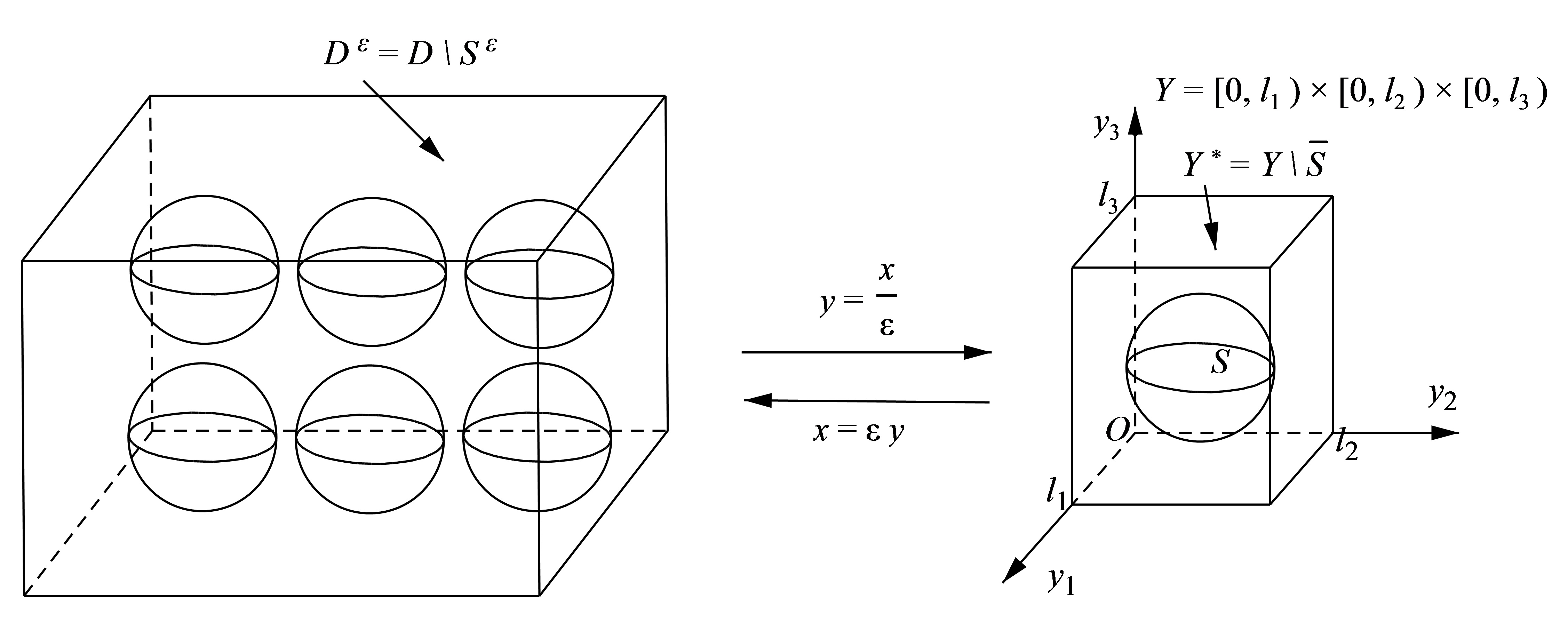
References

  • [1] G. Allaire, Homogenization and two-scale convergence, SIAM J. Math. Anal., 23(1992): 1482-1518.
  • [2] G. Allaire, M. Murat and A. Nandakumar, Appendix of ¡°Homogenization of the Neumann problem with nonisolated holes¡±, Asymptotic Anal., 7(1993): 81-95.
  • [3] J. T. Beale, Spectral properties of an acoustic boundary condition, IndianaUniv. Math. J., 25(1976): 895-917.
  • [4] J. T. Beale, Acoustic scattering from locally reacting surfaces, Indiana Univ. Math. J., 26(1977): 199-222.
  • [5] M. Briane, L. Mazliak, Homogenization of two randomly weakly connected materials, Portugaliae Mathematic, 55(1998): 187-207.
  • [6] G. Chen, J. Duan, and J. Zhang, Geometric shape of invariant manifolds for a class of stochastic partial differential equations, Journal of Mathematical Physics, 52,(2011), 072702.
  • [7] G. Chen and J. Zhang, Asymptotic behavior for a stochastic wave equation with dynamical boundary conditions, Discrete and Continuous Dynamical Systems Series B, 17(2012): 1441-1453.
  • [8] D. Cioranescu and P. Donato, An Introduction to Homogenization, Oxford University Press, New York, 1999.
  • [9] D. Cioranescu, P. Donato, F. Murat and E. Zuazua, Homogenization and correctors results for the wave equation in domains with small holes, Ann. Scuola Norm. Sup. Pisa, 18(1991): 251-293.
  • [10] P. L., Chow, Stochastic wave equations with polynomial nonlinearity, Ann. Appl. Probab., 12(2002): 361-381.
  • [11] P. L. Chow, Asymptotics of solutions to semilinear stochastic wave equations, Ann. Appl. Probab., 16(2006): 757-780.
  • [12] A. T. Cousin, C. L. Frota and N. A. Larkin, Global solvability and asymptotic behavior of a hyperbolic problem with acoustic boundary condition, Funkcialaj Ekvacioj, 44(2001): 471-484.
  • [13] G. Da Prato and J. Zabczyk, Stochastic Equations in Infinite Dimensions, Cambridge University Press, Cambridge, 1992.
  • [14] R. M. Dudley, Real Analysis and Probability, Cambridge University Press, 2002.
  • [15] X. M. Fan, Y.G. Wang, Fractal dimensional of attractors for a stochastic wave equation with nonlinear damping and white noise, Stoch. Anal. Appl., 25(2007): 381-396.
  • [16] S. Frigeri, Attractors for semilinear damped wave equations with an acoustic boundary condition, J. Evol. Equ., 10(2010): 29-58.
  • [17] C. L. Frota and J. A. Goldstein, Some Nonlinear Wave Equations with Acoustic Boundary Conditions, Journal of Differential Equations, 164(2000): 92-109.
  • [18] N. Fusco, G. Moscariello, On the homogenization of quasilinear divergence structure operators, Ann. Math. Pura Appl., 164(1987): 1-13.
  • [19] S. Gerbi and B. Said-Houari, Local existence and exponential growth for a semilinear damped wave equation with dynamic boundary conditions, Advances in Differential Equations, 13(2008): 1051-1074.
  • [20] J. Ginibre and G. Velo, The global Cauchy problem for the nonlinear Klein-Gordon equation, Math. Z., 189(1985): 487-504.
  • [21] M.L. Kleptsyna, A.L. Piatnitski, Homogenization of a random non-stationary convection-diffusion problem, Russ. Math. Surve., 57(2002): 729-751.
  • [22] H. A. Levine, Instability and nonexistence of global solutions to nonlinear wave equations of the form P​ut​t=−A​u+F⁡(u)Pu_{tt}=-Au+F(u), Trans. Amer. Math. Soc., 192(1974): 1-21.
  • [23] K. Lu and B. Schmalfuss, Invariant manifolds for stochastic wave equations, J. Differential Equations, 236(2007): 460-492.
  • [24] Y. Lv, W. Wang, Limiting dynamics for stochastic wave equations, J. Differential Equations, 244(2008): 1-23.
  • [25] P.M. Morse and K.U. Ingard, Theoretical acoustics, McGraw-Hill, New York, 1968.
  • [26] C. Mueller, Long time existence for the wave equation with a noise term, Ann. Probab., 25(1997): 133-151.
  • [27] D. Mugnolo, Abstract wave equations with acoustic boundary conditions, Math. Nachr., 279(2006): 299-318.
  • [28] A.K. Nandakumaran and M. Rajesh, Homogenization of a parabolic equation in a perforated domain with Neumann boundary condition, Proc. Indian Acad. Sci. (Math. Sci.), 112(2002): 195-207.
  • [29] A.K. Nandakumaran and M. Rajesh, Homogenization of a parabolic equation in a perforated domain with Dirichlet boundary condition, Proc. Indian Acad. Sci. (Math. Sci.), 112(2002): 425-439.
  • [30] E. Pardoux, A.L. Piatnitski, Homogenization of a nonlinear random parabolic partial differential equation, Stochastic Process Appl., 104(2003): 1-27.
  • [31] L. E. Payne and D. H. Sattinger, Saddle points and instability of nonlinear hyperbolic equations, Israel J. Math., 22(1975): 273-303.
  • [32] L. Popescu and A. Rodriguez-Bernal, On a singularly perturbed wave equation with dynamic boundary conditions, Proceedings of the Royal Society of Edinburgh, 134A(2004): 389-413.
  • [33] M. Reed and B. Simon, Methods of Modern Mathematical Physics II, Academic Press, New York, 1975.
  • [34] W. A. Strauss, Nonlinear Wave Equations, CBMS Regional Conference Series in Math., 73, Amer. Math. Soc., Providence, RI, 1989.
  • [35] M.B. Taghite, K. Taous and G. Maurice, Heat equations in a perforated composite plate: Influence of a coating, Int J. Eng. Sci., 40(2002): 1611-1645.
  • [36] L. Tartar, The General Theory of Homogenization, Springer-Verlag, Berlin Heidelbeg, 2009.
  • [37] C. Timofte, Homogenization results for a nonlinear wave equation in a perforated domain, U.P.B. Sci. Bull. Series A, 72(2010): 85-92.
  • [38] W. Wang, D. Cao and J. Duan, Effective macroscopic dynamics of stochastic partial differential equations in perforated domains, Siam J. Math. Anal., 38(2007): 1508-1527.
  • [39] W. Wang, J. Duan, Homogenized Dynamics of Stochastic Partial Differential Equations with Dynamical Boundary Conditions, Commun. Math. Phys., 275(2007): 163-186.
  • [40] G. Whitham, Linear and Nonlinear Waves, Wiley, New York, 1974.
  • [41] V.V. Zhikov, On homogenization in random perforated domains of general type, Matem. Zametki, 53(1993): 41-58.
  • [42] V.V. Zhikov, On homogenization of nonlinear variational problems in perforated domains, Russ. J Math. Phys., 2(1994): 393-408.
  • [43] S. F. Zhou, F. Q. Yin, Z. G. Ouyang, Random attractor for damped nonlinear wave equations with white noise, SIAM J. Appl. Dyn. Syst., 4(2005): 883-903.