Strings at Finite Temperature:
Wilson Lines, Free Energies, and the Thermal Landscape
Abstract
According to the standard prescriptions, zero-temperature string theories can be extended to finite temperature by compactifying their time directions on a so-called “thermal circle” and implementing certain orbifold twists. However, the existence of a topologically non-trivial thermal circle leaves open the possibility that a gauge flux can pierce this circle — i.e., that a non-trivial Wilson line (or equivalently a non-zero chemical potential) might be involved in the finite-temperature extension. In this paper, we concentrate on the zero-temperature heterotic and Type I strings in ten dimensions, and survey the possible Wilson lines which might be introduced in their finite-temperature extensions. We find a rich structure of possible thermal string theories, some of which even have non-traditional Hagedorn temperatures, and we demonstrate that these new thermal string theories can be interpreted as extrema of a continuous thermal free-energy “landscape”. Our analysis also uncovers a unique finite-temperature extension of the heterotic and strings which involves a non-trivial Wilson line, but which — like the traditional finite-temperature extension without Wilson lines — is metastable in this thermal landscape.
pacs
11.25.-wI Introduction and motivation
One of the most profound observations in theoretical physics is the relationship between finite-temperature quantum theories and zero-temperature quantum theories which are compactified on a circle. Indeed, the fundamental idea behind this so-called “temperature/radius correspondence” is that the free-energy density of a theory at finite temperature can be reformulated as the vacuum-energy density of the same theory at zero temperature, but with the Euclidean time dimension compactified on a circle of radius . This connection between temperature and geometry is a deep one, stretching from quantum mechanics and quantum field theory all the way into string theory.
This extension to string theory is truly remarkable, given that the geometric compactification of string theory gives rise to numerous features which do not, at first sight, have immediate thermodynamic analogues or interpretations. For example, upon spacetime compactification, closed strings accrue not only infinite towers of Kaluza-Klein “momentum” states but also infinite towers of winding states. While the Kaluza-Kelin momentum states are easily interpreted in a thermal context as the Matsubara modes corresponding to the original zero-temperature states, it is not a priori clear what thermal interpretation might be ascribed to these winding states. Likewise, as a more general (but not unrelated) issue, closed-string one-loop vacuum energies generally exhibit additional symmetries such as modular invariance which transcend field-theoretic expectations. While the emergence of modular invariance is clearly understood for zero-temperature geometric compactifications, the need for modular invariance is perhaps less obvious from the thermal perspective in which one would simply write down a Boltzmann sum corresponding to each string state which survives the GSO projections.
Both of these issues tended to dominate the earliest discussions of string thermodynamics in the mid-1980’s. Historically, they were first flashpoints which seemed to show apparent conflicts between the thermal and geometric approaches which had otherwise been consistent in quantum field theory. However, it is now well understood that there are ultimately no conflicts between these two approaches [1, 2]. Indeed, modular invariance emerges naturally upon relating the integral of the Boltzmann sum over the “strip” in the complex -plane to the integral of the partition function over the fundamental domain of the modular group [3]. Likewise, thermal windings emerge naturally as a consequence of modular invariance and can be viewed as artifacts arising from this mapping between the strip and the modular-group fundamental domain.
There is, however, one additional feature which can generically arise when a theory experiences a geometric compactification: because of the topologically non-trivial nature of the compactification, it is possible for a non-zero gauge flux to pierce the compactification circle. In other words, the compactification might involve a non-trivial Wilson line. Viewed from the thermodynamic perspective, this corresponds to nothing more than the introduction of a chemical potential. However, as we shall see, this is ultimately a rather unusual chemical potential: it is not only imaginary but also temperature-dependent. Such chemical potentials have occasionally played a role in studies of finite-temperature field theory (particularly finite-temperature QCD [4]). However, with only a few exceptions, such chemical potentials (and the Wilson lines to which they correspond) have not historically played a significant role in discussions of finite-temperature string theory.
At first glance, it might seem reasonable to hope (or simply postulate) that Wilson lines should play no role in discussions of finite-temperature string theory. However, Wilson lines play such a critical role in determining the allowed possibilities for self-consistent geometric compactifications of string theory that it is almost inevitable that they should play a significant role in finite-temperature string theories as well. Indeed, the temperature/radius correspondence essentially guarantees this. Thus, it is natural to expect that theories with non-trivial Wilson lines will be an integral part of the full landscape of possibilities for string theories at finite temperature — i.e., that they will be part of the full “thermal string landscape”.
A heuristic argument can be invoked in order to illustrate the connection that might be expected between Wilson lines and string theories at finite temperature. As we know, thermal effects treat bosons and fermions differently and thereby necessarily break whatever spacetime supersymmetry might have existed at zero temperature. However, in string theory there are tight self-consistency constraints which relate the presence or absence of spacetime supersymmetry to the breaking of the corresponding gauge symmetry, and these connections hold even at zero temperature. For example, the heterotic string in ten dimensions is necessarily supersymmetric, and it is inconsistent to break this supersymmetry without simultaneously introducing a non-trivial Wilson line (or in this context, a gauge-sensitive orbifold twist) which also breaks the gauge group. Indeed, the two are required together. Even for the gauge group, a similar situation arises: although there exist two heterotic strings, one supersymmetric and the other non-supersymmetric, the orbifold which relates them to each other is not simply given by the SUSY-breaking action , where is the spacetime fermion number. Rather, the required orbifold which twists the supersymmetric heterotic string to become the non-supersymmetric heterotic string is given by where is a special non-zero Wilson line which acts non-trivially on the gauge degrees of freedom. This example will be discussed further in Sect. IV. Indeed, such a Wilson line is needed even though we are not breaking the gauge symmetry in passing from our supersymmetric original theory to our final non-supersymmetric theory. Such examples indicate the deep role that Wilson lines play in zero-temperature string theory, and which they might therefore be expected to play in a finite-temperature context as well.
In this paper, we shall undertake a systematic examination of the role that such Wilson lines might play in string thermodynamics. We shall concentrate on the zero-temperature heterotic and Type I strings in ten dimensions, and survey the possible Wilson lines which might be introduced in their finite-temperature extensions. As we shall see, this gives rise to a rich structure of possible thermal string theories, and we shall demonstrate that these new thermal string theories can be interpreted as extrema of a continuous thermal free-energy “landscape”. In fact, some of these new thermal theories even have non-traditional Hagedorn temperatures, an observation which we shall discuss (and explain) in some detail. Our analysis will also uncover a unique finite-temperature extension of the heterotic and strings which involves a non-trivial Wilson line, but which — like the traditional finite-temperature extension without Wilson lines — is metastable in this thermal landscape. Such new theories might therefore play an important role in describing the correct thermal vacuum of our universe.
This paper is organized as follows. In order to set the stage for our subsequent analysis, in Sect. II we provide general comments concerning string theories at finite temperature and in Sect. III we discuss the possible role that Wilson lines can play in such theories. We also discuss the equivalence between such thermal Wilson lines and temperature-dependent chemical potentials. In Sect. IV, we then survey the specific Wilson lines that may self-consistently be introduced when constructing our thermal theories, concentrating on the two supersymmetric heterotic strings in ten dimensions as well as the supersymmetric Type I string in ten dimensions. In Sect. V, we demonstrate that non-trivial Wilson lines can also affect the Hagedorn temperatures experienced by these strings, and show how such shifts in the Hagedorn temperature can be reconciled with the asymptotic densities of the zero-temperature bosonic and fermionic string states. Then, in Sect. VI, we extend our discussion in order to consider continuous thermal Wilson-line “landscapes” for both heterotic and Type I strings. It is here that we discuss which Wilson lines lead to “stable” and/or “metastable” theories. Finally, in Sect. VII, we conclude with some general comments and discussion. An Appendix summarizes the notation and conventions that we shall be using throughout this paper.
II Strings at finite temperature
We begin by discussing the manner in which a given zero-temperature string model can be extended to finite temperature. This will also serve to establish our conventions and notation. Because of its central role in determining the thermodynamic properties of the corresponding finite-temperature string theory, we shall focus on the calculation of the one-loop string thermal partition function . The situation is slightly different for closed and open strings, so we shall discuss each of these in turn.
II.1 Closed strings
In order to begin our discussion of closed strings at finite temperature, we begin by reviewing the case of a one-loop partition function for a closed string at zero temperature. Our discussion will be as general as possible, and will therefore apply to all closed strings, be they bosonic strings, Type II superstrings, or heterotic strings. For closed strings, the one-loop partition function is defined as
| (1) |
where the trace is over the complete Fock space of states in the theory, weighted by a spacetime statistics factor . Here where is the one-loop (torus) modular parameter, and denote the worldsheet energies for the right- and left-moving worldsheet degrees of freedom, respectively. Note that in general, is the quantity which appears in the calculation of the one-loop cosmological constant (vacuum-energy density) of the model:
| (2) |
where is the number of uncompactified spacetime dimensions, where is the reduced string scale, and where
| (3) |
is the fundamental domain of the modular group. Of course, the quantity in Eq. (2) is divergent for the compactified bosonic string as a result of the physical bosonic-string tachyon.
Given the general form for the zero-temperature one-loop string partition function in Eq. (1), it is straightforward to construct its generalization to finite temperature. As is well known in field theory, the free-energy density of a boson (fermion) in spacetime dimensions at temperature is nothing but the zero-temperature vacuum-energy density of a boson (fermion) in spacetime dimensions, where the (Euclidean) timelike dimension is compactified on a circle of radius about which the boson (fermion) is taken to be periodic (anti-periodic). We shall refer to this observation as the “temperature/radius correspondence”. This correspondence generally extends to string theory as well [1, 2], state by state in the string spectrum. However, for closed strings there is an important extra ingredient: we must include not only the “momentum” Matsubara states that arise from the compactification of the timelike direction, but also the “winding” Matsubara states that arise due to the closed nature of the string. Indeed, both types of states are necessary for the modular invariance of the underlying theory at finite temperature. As a result, a given zero-temperature string state will accrue not a single sum of Matsubara/Kaluza-Klein modes at finite temperature, but actually a double sum consisting of the Matsubara/Kaluza-Klein momentum modes as well as the Matsubara winding modes.
The final expressions for our finite-temperature string partition functions must also be modular invariant, satisfying the constraint . Because our thermal theory necessarily includes two groups of momentum quantum numbers (namely those with as well as those with ) which are treated separately (corresponding to spacetime bosons and fermions respectively), modular invariance turns out to imply that winding numbers which are even will likewise be treated separately from those that are odd. As a result, the most general thermal string-theoretic partition function will take the form [5, 6, 7, 8]
| (4) | |||||
Here and represent the thermal portions of the partition function, namely the double sums over appropriate combinations of thermal momentum and winding modes [5]. Specifically, the functions include the contributions from even winding numbers along with either integer or half-integer momenta , while the functions include the contributions from odd winding numbers with either integer or half-integer momenta . These functions are defined explicitly in the Appendix. Likewise, the terms () represent the traces over those subsets of the zero-temperature string states in Eq. (1) which accrue the corresponding thermal modings at finite temperature. For example, represents a trace over those string states in Eq. (1) which accrue even thermal windings and integer thermal momenta , and so forth. Modular invariance for as a whole is then achieved by demanding that each transform exactly as does its corresponding function.
In the limit, it is easy to verify that and each vanish while with . As a result, we find that
| (5) |
The divergent prefactor proportional to in Eq. (5) is a mere rescaling factor which reflects the effective change of the dimensionality of the theory in the limit. Specifically, this is an expected dimensionless volume factor which emerges as the spectrum of surviving Matsubara momentum states becomes continuous. However, we already know that in Eq. (1) is the partition function of the zero-temperature theory. As a result, we can relate Eqs. (1) and (4) by identifying
| (6) |
We see, then, that the procedure for extending a given zero-temperature string model to finite temperature is relatively straightforward. Any zero-temperature string model is described by a partition function , the trace over its Fock space. The remaining task is then simply to determine which states within are to accrue integer modings around the thermal circle, and which are to accrue half-integer modings. Those that are to accrue integer modings become part of , while those that are to accrue half-integer modings become part of . In this way, we are essentially decomposing in Eq. (6) into separate components and . Once this is done, modular invariance alone determines the unique resulting forms for and . The final thermal partition function is then given in Eq. (4). In complete analogy to Eq. (2), we can then proceed to define the -dimensional vacuum-energy density
| (7) |
(where ), whereupon the corresponding -dimensional free-energy density is given by
| (8) |
As we see from this discussion, the only remaining critical question is to determine how to decompose as in Eq. (6) into the pieces and — i.e., to determine which states within are to accrue integer thermal modings (and thereby be included within ), and which are to accrue half-integer modings (and thereby be included within ). However, this too is relatively simple. In general, a given string model will give rise to states which are spacetime bosons as well as states which are spacetime fermions. In making this statement, we are identifying “bosons” and “fermions” on the basis of their spacetime Lorentz spins. (By the spin-statistics theorem, this is equivalent to identifying these states on the basis of their Bose-Einstein or Fermi-Dirac quantizations.) As a result, we can always decompose into separate contributions from spacetime bosons and spacetime fermions:
| (9) |
However, the temperature/radius correspondence instructs us that bosons should be periodic around the thermal circle, and fermions should be anti-periodic around the thermal circle. In the absence of any other effects, a field which is periodic around the thermal circle will have integer momentum quantum numbers , while a field which is anti-periodic will have half-integer momentum quantum numbers . Thus, given the decomposition in Eq. (9), the standard approach which is taken in the string literature is to identify
| (10) |
This makes sense, since corresponds to the sector which accrues integer thermal Matsubara modes while corresponds to the sector which accrues half-integer thermal Matsubara modes . Indeed, the choice in Eq. (10) is the unique choice which reproduces the standard Boltzmann sum for the states in the string spectrum.
We can illustrate this procedure by explicitly writing down the standard thermal partition functions for the ten-dimensional supersymmetric and heterotic strings at finite temperature. At zero temperature, both of these string theories have partition functions given by
| (11) |
where denotes the contribution from the eight worldsheet bosons and where the contributions from the right-moving worldsheet fermions are written in terms of the barred characters of the transverse Lorentz group. These quantities are defined in the Appendix. By contrast, denotes the contributions from the left-moving (internal) worldsheet degrees of freedom. Written in terms of products of the unbarred characters of the gauge group, these left-moving contributions are given by
| (12) |
States which are spacetime bosons or fermions contribute to the terms in Eq. (11) which are proportional to or , respectively. The standard Boltzmann prescription in Eq. (10) therefore leads us to identify
| (13) |
whereupon modular invariance requires that
| (14) |
We therefore obtain the thermal partition functions
| (15) |
This is indeed the standard result in the string literature [7].
II.2 Type I strings
We now turn to the case of Type I strings. Such strings, of course, have both closed and open sectors. Because Type I strings are unoriented, their one-loop vacuum vacuum energies receive four separate contributions: those from the closed-string sectors have the topologies of a torus and a Klein bottle, while those from the open-string sectors have the topologies of a cylinder and a Möbius strip. We therefore must consider four separate partition functions: , , , and .
At zero temperature, both and are traces over the closed-string states in the theory:
| (16) |
where is the orientation-reversing operator which exchanges left-moving and right-moving worldsheet degrees of freedom. Thus, taken together, the sum represents a single trace over those closed-string states which are invariant under , as appropriate for an unoriented string. Note that because of the presence of the orientifold operator within , the Klein-bottle contribution can ultimately be represented as a power series in terms of a single variable where represents the modulus for double-cover of the torus, as given in Eq. (111). Likewise, corresponding to this are the traces over the open-string states in the theory:
| (17) |
where is the open-string worldsheet energy and where with defined in Eq. (111). The presence of within guarantees that represents a single trace over an orientifold-invariant set of open-string states.
Extending these contributions to finite temperatures is also straightforward. The extension of the torus contribution to finite temperatures proceeds exactly as discussed above for closed strings, ultimately leading to an expression of the same form as in Eq. (4), with four different thermal sub-contributions . The corresponding finite-temperature Klein-bottle contributions can be derived from the finite-temperature torus contribution by implementing the orientifold projection in the finite-temperature trace, ultimately leading to an expression which can be recast in the form
| (18) |
where the thermal functions and are defined in Eq. (107) and serve as the open-string analogues of the closed-string thermal functions. Likewise, the open-string sector extends to finite temperatures in complete analogy with the closed-string sector, by associating certain states with and others with :
| (19) |
Note that and become equal as . It therefore follows that for .
Once these four partition functions are determined, the corresponding free-energy density is easily calculated. The contribution from the torus to the free-energy density is given by
| (20) |
in complete analogy with Eqs. (7) and (8). By contrast, the remaining contributions to the free-energy density are each given by
| (21) |
The total free-energy density of the thermal string model is then given by
| (22) |
Thus, just as for closed strings, we see that the art of extending a given zero-temperature Type I string theory to finite temperatures ultimately boils down to choosing the manner in which the zero-temperature partition functions and are to be decomposed into the separate thermal contributions and respectively. Once these choices are made, the rest follows uniquely: modular invariance dictates , and orientifold projections determine and . Moreover, just as for closed strings, it turns out that the traditional Boltzmann sum is reproduced in the finite-temperature theory by making the particular choices for and such that the spacetime bosonic (fermionic) states within and are associated with () and () respectively.
To illustrate this procedure, let us consider the single self-consistent zero-temperature ten-dimensional Type I string model which is both supersymmetric and anomaly-free: this is the Type I string [1]. Note that this string can be realized as the orientifold projection of the ten-dimensional zero-temperature Type IIB superstring, whose partition function is given by
| (23) |
Here denotes the contribution from the eight worldsheet coordinate bosons, just as for the heterotic strings discussed above, and the contributions from the left-moving (right-moving) worldsheet fermions are written in terms of the holomorphic (anti-holomorphic) characters () of the transverse Lorentz group. Implementing the orientifold projection is relatively straightforward, and leads to the Type I contributions
| (24) |
where we have used the notation and conventions defined in the Appendix. Tadpole anomaly cancellation ultimately requires that we take , thereby leading to the gauge group. Note that while the cylinder contribution scales as [representing the sum of the dimensionalities of the symmetric and anti-symmetric tensor representations of ], the Möbius contribution scales only as (representing their difference).
Given the results for the zero-temperature Type I theory in Eq. (24), it is straightforward to construct their finite-temperature extension. Within the torus contribution in Eq. (24), we recognize that the states which are spacetime bosons are those which contribute to , while those that are spacetime fermions contribute to . Following the standard Boltzmann description, we thus identify
| (25) |
Similar reasoning for the cylinder contribution in Eq. (24) also leads us to identify
| (26) |
Given these choices, the remaining terms in the total thermal partition function are determined through modular transformations and orientifold projections, leading to the final finite-temperature result
| (27) |
This, too, is the standard result in the string-thermodynamics literature.
III Wilson lines and imaginary chemical potentials
As we have seen in the previous section, there is a simple procedure by which a given zero-temperature string model can be extended to finite temperatures. Indeed, because of constraints coming from modular invariance and/or orientifold projections, we have relatively little choice in how this is done. For closed strings, the only freedom we have is related to how our (torus) partition function is decomposed into and — i.e., into the separate contributions that determine which of the zero-temperature states in the theory are to receive integer modings around the thermal circle, and which states are to receive half-integer modings . Likewise, for Type I strings, we have an additional freedom which concerns how the same choice is ultimately made for the open-string sectors. However, once those choices are made, all of the resulting thermal properties of the theory are completely determined.
As discussed in the previous section, the standard prescription is to identify those states which are spacetime bosons with integer modings around the thermal circle, and those which are spacetime fermions with half-integer modings . Indeed, this is ultimately the unique choice for which the resulting string partition functions correspond to the standard field-theoretic Boltzmann sums for each string state (a fact which is most directly evident after certain Poisson resummations are performed, essentially transforming our theory from the so-called -representation we are using here to the so-called -representation in which the modular invariance of the torus contributions is not manifest).
Given this observation, it might seem that there is therefore no choice in how our zero-temperature string theories are extended to finite temperatures. However, this is not entirely correct. It is certainly true that the temperature/radius correspondence instructs us to treat bosonic states as periodic around the thermal circle and fermionic states as anti-periodic. However, this does not necessarily imply that all bosonic states will correspond to integer momentum modings , or that all fermionic states will correspond to half-integer momentum modings . Indeed, in the presence of a non-trivial Wilson line, this result can change.
In order to understand how this can happen, let us first recall how the standard “temperature/radius correspondence” is derived (see, e.g., Ref. [9]). As is well known, this correspondence is most directly formulated in quantum field theory (as opposed to string theory) and ultimately rests upon the algebraic similarity between the free-energy density of a thermal theory and the vacuum-energy density of the zero-temperature theory in which the Euclidean timelike direction is geometrically compactified on a circle. This similarity can be demonstrated as follows. Let us begin on the thermal side, and consider the thermal (grand-canonical) partition functions corresponding to a single real -dimensional bosonic field and a single -dimensional fermionic field of mass :
| (28) |
with . In Eq. (28), the products are over all -dimensional spatial momenta . Given these thermal partition functions, the corresponding -dimensional free-energy densities are given by
| (29) |
However, thanks to certain infinite-product representations for the hyperbolic trigonometric functions, it is an algebraic identity that
| (30) |
where and . In writing Eq. (30), we have followed standard practice and dropped terms beyond the infinite products as well as terms which compensate for the dimensionalities of the arguments of the logarithms. We therefore find that
| (31) |
On the zero-temperature side, by contrast, we can consider the zero-point one-loop vacuum-energy density corresponding to a single real quantum field of mass in uncompactified dimensions:
| (32) |
Here indicates the spacetime statistics of the quantum field ( for a bosonic field, for a fermionic field). Moreover, if we imagine that the time dimension is compactified on a circle of radius (so that the integral over can be replaced by a discrete sum), and if the quantum field in question is taken to be periodic (P) or anti-periodic (A) around this compactification circle, then Eq. (32) takes the form
| (33) |
where , . Given these results, it is now possible to make the “temperature/radius correspondence”: comparing Eq. (31) with Eq. (33), we see that we can identify the free-energy density of a boson (fermion) in spacetime dimensions at temperature with the zero-temperature vacuum-energy density of a boson (fermion) in spacetime dimensions, where a (Euclidean) timelike dimension is compactified on a circle of radius about which the boson (fermion) is taken to be periodic (anti-periodic).
Given this derivation of the temperature/radius correspondence, it may at first glance seem that the identification of bosons and fermions with integer and half-integer modings around the thermal circle is sacrosanct. However, let us consider what happens when we repeat this derivation in the presence of a non-trivial gauge field on the geometric (zero-temperature) side. When we calculate the vacuum energies of our bosonic or fermionic quantum field in the presence of a non-trivial gauge field , we must use the kinematic momenta where is the charge (expressed as a vector in root space) of the field in question. Of course, if the field is pure-gauge (i.e., with vanishing corresponding field strength) and our spacetime geometry is trivial, then this change in momenta from to will have no physical effect. However, if we are compactifying on a circle, there is always the possibility that our compactification encloses a gauge-field flux. As in the Aharonov-Bohm effect, this then has the potential to introduce a non-trivial change in modings for fields around this circle, even if the gauge field is pure-gauge at all points along the compactification circle. Indeed, such a flat (pure-gauge) background for the gauge field is nothing but a Wilson line.
To be specific, let us first consider the situation in which our compactification circle of radius completely encloses a magnetic flux of magnitude which is entirely contained within a radius . At all points along the compactification circle, this then corresponds to a gauge field whose only non-zero component is the component along the compactified dimension. Because of the non-trivial topology of the circle, we then find that the shift from to for a state with charge induces a corresponding shift in the corresponding modings:11 1 This discussion of the effects of Wilson lines is mostly field-theoretic. For closed strings, however, there will also be an additional shift due to the possible appearance of a non-trivial winding number. This will be discussed below, but we shall disregard these additional shifts here since since they play no essential role in the present discussion.
| (34) |
While this result holds for gauge fields, it is easy to generalize this to the gauge fields of any gauge group . For any gauge group , we can describe a corresponding gauge flux in terms of the parameters for each , where is the rank of . Collectively, we can write as a vector in root space. Likewise, the gauge charge of any given state can be described in terms of its Cartan components for ; collectively, is nothing but the weight of the state in root space. We then find that the modings are shifted according to
| (35) |
As a result, complex fields which are chosen to be periodic (P) or anti-periodic (A) around the compactification circle will have vacuum energies given by
| (36) |
where . Note that in each case, the underlying periodicity properties of the field are unaffected. Rather, it is the manifestations of these periodicities in terms of the modings which are affected by the appearance of the Wilson line.
This, then, explains how a non-trivial Wilson line can produce unexpected modings due to the non-trivial compactification geometry. However, we still wish to understand the appearance of such a Wilson line thermally. What is the thermal analogue of the non-trivial Wilson line? Or, phrased somewhat differently, what effect on the thermal side can restore the temperature/radius correspondence if a non-trivial Wilson line has been introduced on the geometric side?
It turns out that introducing a non-trivial Wilson line on the geometric side corresponds to introducing a non-zero chemical potential on the thermal side. In fact, this chemical potential will be imaginary. To see this, let us reconsider the partition functions of complex bosons and fermions in the presence of a non-zero chemical potential where . In general, a complex bosonic field will have a grand-canonical partition function given by
| (37) |
where the two factors in Eq. (37) correspond to particle and anti-particle excitations respectively. The corresponding free energy then takes the form
| (38) | |||||
In Eq. (38), the second equality follows from the algebraic identities in Eq. (30) while the final equality results upon exchanging in the second term. Thus, comparing the result in Eq. (38) with the result in Eq. (36), we see that the free energy of a bosonic field at temperature is equal to the vacuum energy of a periodically-moded field on a circle of radius , where and where
| (39) |
A similar result holds for complex fermions and anti-periodic fields, with the same chemical potential. We thus conclude that the introduction of a non-trivial Wilson line on the geometric side corresponds to the introduction of an imaginary, temperature-dependent chemical potential on the thermal side. This result is well known in field theory [4], and has also recently been discussed in a string-theory context [10].
Before concluding, we should remark that the above discussion has been somewhat field-theoretic. Indeed, if we define the Wilson-line parameter
| (40) |
then our primary result is that a non-trivial Wilson line induces a shift in the momentum quantum number of the form
| (41) |
for a state carrying charge with respect to the gauge field constituting the Wilson line. This result is certainly true in quantum field theory, and also holds by extension for open-string states. However, closed-string states can carry not only momentum quantum numbers but also winding numbers which parametrize their windings around the thermal circle. This is important, because in the presence of a non-zero winding mode , a non-trivial Wilson line shifts not only the momentum but also the charge vector of a given state, so that Eq. (41) is generalized to [11]
| (42) |
IV Surveying possible Wilson lines
We have already seen in Sect. II that the manner in which a zero-temperature string theory is extended to finite temperature depends on the choice as to which zero-temperature states are to be associated with integer momenta around the thermal circle, and which are to be associated with half-integer momenta . Once this decision is made, the thermal properties of the resulting theory are completely fixed. Moreover, we have seen in Sect. III that there is considerable freedom in making this choice, depending on whether (and which) Wilson lines might be present. Indeed, in principle, each choice of Wilson line leads to an entirely different thermal theory. While all of these thermal theories necessarily reduce back to the starting zero-temperature theory as , they each represent different possible finite-temperature extensions of that theory which correspond to different possible chemical potentials which might be introduced into their corresponding Boltzmann sums. Indeed, viewed from this perspective, we see that the traditional Boltzmann choices merely correspond to one special case: that without a Wilson line, for which the corresponding chemical potential vanishes.
As an example, let us consider the supersymmetric heterotic string. At zero temperature, the partition function of this theory is
| (43) |
and without a Wilson line we would normally decompose this into the separate thermal contributions and by making the associations
| (44) |
Indeed, this is precisely the decomposition discussed in Sect. II, which leads to the standard Boltzmann sum. However, there are in principle other ways in which the zero-temperature partition function in Eq. (43) might be meaningfully decomposed. For example, let us consider an alternate decomposition of the form
| (45) |
Unlike the standard Boltzmann decomposition, this alternate decomposition treats spacetime bosonic and fermionic states in ways which are also dependent on their corresponding gauge quantum numbers. Specifically, while vectorial representations of the gauge group are treated as expected, with spacetime bosons having integer momentum modings and spacetime fermions having half-integer momentum modings , the spinorial representations of the left-moving gauge group have the opposite behavior, with spacetime bosons associated with modings and spacetime fermions associated with modings . [Note, in this connection, that the character combination is nothing but the character , and likewise is nothing but .] However, as we have seen in Sect. III, such “wrong” modings can be easily understood as the effects of a non-trivial Wilson line. Indeed, looking at Eq. (42), we see that the results in Eq. (45) are obtained directly if our Wilson line is chosen such that (mod ) for states in spinorial representations of , while (mod ) for states in vectorial representations of . Given that for vectorial representations of and for spinorial representations of , we see that a simple choice such as can easily accomplish this.
However, at this stage, we have no knowledge as to whether or not such a Wilson line represents a legitimate choice for the heterotic string. For example, we have no idea whether such a Wilson-line choice is compatible with a worldsheet interpretation in which the possible choices of Wilson lines are tightly constrained by numerous string self-consistency constraints. Moreover, along the same lines, we do not know what other Wilson lines might also be available.
In order to explore all of the potential possibilities, we shall therefore proceed to survey the set of all possible Wilson lines which might be self-consistently introduced when attempting to extend a given zero-temperature string theory to finite temperatures. As we shall see, however, the situation is somewhat different for closed strings and Type II strings. We shall therefore consider these two cases separately.
IV.1 Closed strings
In general, there are two classes of closed strings which are supersymmetric and hence perturbatively stable: Type II superstrings and heterotic strings. In ten dimensions, however, the Type II superstrings lack gauge symmetries; thus no possible Wilson lines can exist in their extensions to finite temperatures. For this reason, when discussing closed strings, we shall concentrate on the ten-dimensional supersymmetric and heterotic strings. Note, however, that in lower dimensions, all of the closed strings will accrue additional gauge symmetries as a result of compactification — indeed, this holds for Type II strings as well as heterotic. Thus, in lower dimensions, the sets of allowed Wilson lines in each case are likely to be much more complex than we are considering here.
In general, the temperature/radius correspondence provides us with a powerful tool to help determine the allowed Wilson lines that may be introduced when forming our thermal theory: we simply replace the temperature with and consider the corresponding problem of introducing a Wilson line into the geometric compactification of our original zero-temperature theory. For example, if we are seeking the set of allowed Wilson lines that can be introduced into the construction of the finite-temperature ten-dimensional heterotic theory, we can instead investigate the allowed Wilson lines that may be introduced upon compactifying the zero-temperature theory to nine dimensions. In principle, the latter problem can be studied through any number of formalisms having to do with the construction of self-consistent zero-temperature string models — such model-building formalisms are numerous and include various orbifold constructions, Narain lattice constructions, constructions based on free worldsheet bosons and fermions, and so forth.
However, for closed strings, it turns out that T-duality leads to a significant simplification: while the (or ) limit reproduces our original string model in the original spacetime dimensions, and while taking leads to a string model in spacetime dimensions, the formal (or ) limit actually yields a new string theory which is back in spacetime dimensions! Moreover, the structure of the finite-temperature string partition function in Eq. (4) guarantees that this new -dimensional theory is nothing but a orbifold of our original -dimensional theory; indeed, while the original theory in the limit has the partition function , the final theory in the limit has the partition function . In some sense, the thermal theory in dimensions interpolates between the original -dimensional theory at and a different -dimensional theory as , these two -dimensional theories being orbifolds of each other. Thus, the allowed Wilson lines that may be introduced into the finite-temperature extension of a given zero-temperature closed string theory are in one-to-one correspondence11 1 At a technical level, this correspondence is easy to understand. Starting from a given zero-temperature theory in dimensions, one may construct the corresponding thermal theory through a specific sequence of steps: first, one compactifies the zero-temperature theory on a circle of radius , and then one orbifolds the resulting theory by the action where is the spacetime fermion number, where denotes a half-shift around the thermal circle, and where (the Wilson line) indicates an additional specific orbifold action which is sensitive to the gauge quantum numbers of each state. The resulting -dimensional thermal theory then has the property that the original -dimensional theory is reproduced as , and that a new -dimensional theory emerges in the formal limit. Moreover, it can also be shown that the new theory which emerges in the limit is a orbifold of the original theory, where the orbifold in this case is nothing but . Thus, for each Wilson line which is involved in construction of the thermal theory in -dimensions, there is a corresponding orbifold which directly relates the two “endpoint” -dimensional theories to each other. with the set of allowed orbifolds of that theory — i.e., the set of orbifolds which reproduce another self-consistent string theory in dimensions.
This correspondence provides us with exactly the tool we need, because the complete set of self-consistent heterotic string theories in ten dimensions is known. Indeed, these have been classified in Ref. [12], and it turns out that in addition to the supersymmetric and heterotic theories, there are only seven additional heterotic theories in ten dimensions. These are the tachyon-free string model [13, 14] as well as six tachyonic string models with gauge groups , , , , , and .
However, not all of these models can be realized as orbifolds of the original supersymmetric or models. Indeed, of the seven non-supersymmetric models listed above, only four are orbifolds of the supersymmetric string; likewise, only four are orbifolds of the string. These orbifold relations are shown in Fig. 1.
It is important to note that there also exists a non-trivial orbifold relation which directly relates the supersymmetric and strings to each other. However, it is easy to see that this orbifold must be excluded from consideration. On the thermal side, we know that finite-temperature effects necessarily treat bosons and fermions differently and will therefore necessarily break whatever spacetime supersymmetry might have existed at zero temperature. This implies that we must restrict our attention to those orbifolds which project out whatever gravitino might have existed in our original -dimensional model. The orbifold relating the supersymmetric and strings to each other does not have this property. Likewise, there also exists a non-trivial orbifold [specifically ] which maps the supersymmetric and heterotic strings to chirality-flipped versions of themselves. This somewhat degenerate orbifold actually corresponds to the situation without a Wilson line, and has thus already been implicitly considered in Eq. (15).

Given these results, we see that there are only four non-trivial candidate Wilson-line choices for the finite-temperature heterotic string. Likewise, there are only four candidate Wilson-line choices for the finite-temperature heterotic string. For each of these Wilson-line choices, we can then construct the corresponding finite-temperature theory.
It is straightforward to write down the partition functions of these finite-temperature theories, some of which have already appeared in various guises in previous work (see, e.g., Refs. [5, 15, 16]). In each case, we shall follow the exact notations and conventions established in the Appendix. However, for convenience, we shall also establish one further convention. Although the anti-holomorphic (right-moving) parts of these partition functions will always be expressed in terms of the (barred) characters of the transverse Lorentz group, it turns out that we can express the holomorphic (left-moving) parts of each of these partition functions in terms of the (unbarred) characters associated with the group . Indeed, it turns out that such a rewriting is possible in each case regardless of the actual gauge group of the ten-dimensional model that is produced by the orbifold. Of course, if is a subgroup of , then such a rewriting is meaningful and the characters which appear in the resulting partition function correspond to the actual gauge-group representations which appear in spectrum of the model. By contrast, if is not a subgroup of , then such a rewriting is merely an algebraic exercise; the characters then have no meaning beyond their -expansions, and can appear with non-integer coefficients. In all cases, however, these expressions represent the true partition functions of these thermal theories as far as their -expansions are concerned. We shall therefore follow these conventions in what follows.
Let us begin by considering the zero-temperature supersymmetric heterotic string, which has the partition function given in Eq. (43). For this string, our four possible finite-temperature extensions are then as follows. In each case we shall label each of the possibilities according to the model produced by the corresponding orbifold. The partition function of the thermal model associated with the orbifold producing the non-supersymmetric heterotic string is given by
| (46) | |||||
while the partition functions of the thermal models associated the orbifolds that produce the the , , and models are respectively given by
| (47) | |||||
| (48) | |||||
and
| (49) | |||||
Note that as , each of these expressions reduces to the partition function of the zero-temperature supersymmetric heterotic string in Eq. (43), as required.
As is easy to verify, these four different thermal extensions of the supersymmetric heterotic string correspond to the Wilson lines
| (50) |
Indeed, because our original supersymmetric heterotic theory contains only vectorial and spinorial representations of , each of the individual components of the Wilson line is defined only modulo 2.
A similar situation exists for the zero-temperature heterotic string, which has partition function
| (51) |
The partition function of the thermal extension of this model associated with the orbifold producing the non-supersymmetric model is given by
| (52) | |||||
while the partition functions of the thermal models associated with the , , and orbifolds are respectively given by
| (53) | |||||
| (54) | |||||
and
| (55) | |||||
Once again, using the identities listed in the Appendix, it is straightforward to verify that each of these expressions reduces to Eq. (51) as . Moreover, the expressions in Eqs. (49) and (55) are actually equal as the result of the further identity on characters given by
| (56) |
This is ultimately the identity which is responsible for the fact that the two expressions within Eq. (12) are equal at the level of their -expansions, i.e., that the ten-dimensional supersymmetric and heterotic strings have the same bosonic and fermionic state degeneracies at each mass level.
As an aside, it is interesting to note that all of these thermal functions can be written in a common form parametrized by a single integer :
| (57) | |||||
In particular, the values correspond to the partition functions in Eqs. (46), (52), (47), (53), (48), (54), and (49) [or (55)] respectively, where Eq. (56) has been used wherever needed.
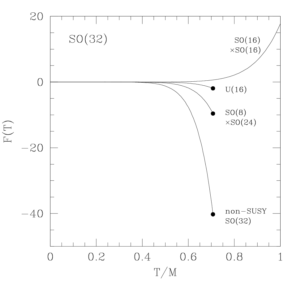
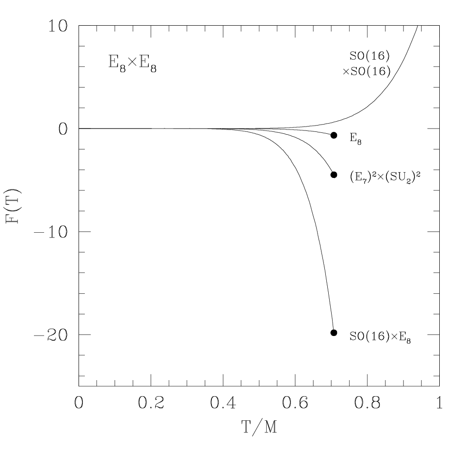
It is also instructive to examine the free-energy densities associated with each of these possible Wilson-line choices. As we have seen, for each thermal partition function listed above, the corresponding free-energy density is given by Eq. (8). Following this definition, we then obtain the results shown in Fig. 2.
We observe from Fig. 2 that the non-trivial Wilson line which minimizes the free-energy density in each case is the one which breaks the gauge group minimally. For the string, this is the Wilson line associated with the non-supersymmetric orbifold, while for the heterotic string, this is the Wilson line associated with the non-supersymmetric orbifold. It is tempting to say, therefore, that these particular non-trivial Wilson lines are somehow “preferred” in some dynamical sense over the others. However, this assumption presupposes the existence of a mechanism by which these Wilson lines can smoothly be deformed into each other with finite energy cost. Given that these Wilson lines ultimately correspond to fluxes which are not only constrained topologically but also presumably quantized, such Wilson-line-changing transitions would require exotic physics (such as might occur on a full thermal landscape). We shall discuss the structure of such a landscape in Sect. VI. We also note that for both of our supersymmetric heterotic strings, there remains the traditional option of constructing a thermal theory without a non-trivial Wilson line. It turns out that the free energies corresponding to these choices are numerically almost identical (but ultimately slightly smaller) than those of the non-supersymmetric and cases plotted in Fig. 2. These features will be discussed further in Sect. VI.
We see, then, that have been able to construct four new thermal theories for the supersymmetric heterotic string as well as four new thermal theories for the supersymmetric heterotic string. Each of these theories has the novel feature that a non-trivial Wilson line has been introduced when constructing the finite-temperature extension, or equivalently that a non-trivial temperature-dependent chemical potential has been introduced into the Boltzmann sum. Each of these theories reduces to the correct supersymmetric theory as , and moreover each is modular invariant for all temperatures . Even more importantly, the temperature/radius correspondence guarantees that in each case, the temperature variable — like the radius variable to which it corresponds — is a bona-fide modulus of the theory, able to be freely changed without disturbing the worldsheet self-consistency of the string. Despite the fact that the non-trivial Wilson lines we have introduced in each case have led to certain unorthodox modings for our string states around the thermal circle, none of these theories violates any spin-statistics relations. Indeed, the spin-statistics theorem relates the spacetime Lorentz spin of a given quantum field to its thermal statistics, and the temperature/radius correspondence relates such thermal statistics to the periodicity of such a field around the thermal circle. Indeed, it is only the relation between this periodicity and the resulting algebraic moding which is altered as a result of the non-trivial Wilson line.
IV.2 Type I strings
We now turn our attention to the corresponding situation for Type I strings. In ten dimensions, there is a single self-consistent Type I string model which is both supersymmetric and anomaly-free: this is the Type I string [1]. Our goal is therefore to survey the possible Wilson lines which can be introduced when formulating its thermal extension.
As discussed in Sect. II, the ten-dimensional zero-temperature Type I string has a partition function given in Eq. (24), and its extension to finite temperature without Wilson lines is given in Eq. (27). However, just as for the heterotic strings, we expect that new thermal possibilities can be constructed when non-trivial Wilson lines are introduced [16, 17, 18].
In general, as discussed in Sect. II, there are two kinds of Wilson lines which might be introduced for Type I theories. First, there are Wilson lines that might be introduced into the closed-string sectors of such theories, much along the lines we have already discussed for the heterotic strings. However, the closed-string sectors of Type I strings are essentially Type II superstrings (indeed, these are the strings from which the Type I strings can be obtained by orientifolding), and in ten dimensions the perturbative states of such Type II strings do not carry gauge charges. Thus, for the ten-dimensional Type I string, it is not possible to introduce a non-trivial Wilson line in the closed-string sector. This guarantees that the results for and given in Eq. (27) will remain invariant regardless of what happens in the open-string sector.
The question then boils down to determining the allowed Wilson lines that might be introduced in the open-string sector of the ten-dimensional Type I string. Indeed, because the states contributing to the cylinder and Möbius partition functions carry gauge charges, their modings in Eq. (27) are potentially affected by the presence of an Wilson line. Fortunately, thanks to the temperature/radius correspondence, this problem can be mapped to the purely geometric issue of determining the allowed Wilson lines that can be introduced when compactifying the Type I string to nine dimensions on a circle — indeed, the fact that we continually refer to “Wilson lines” and “thermal circles” already implicitly presupposes that this can be done! It turns out that the allowed Wilson lines fall into two distinct classes.
The first class consists of Wilson lines of the form
| (58) |
where the number of non-zero components is given by , with . The special case corresponds to the case without a Wilson line, and in general we shall define and . For Wilson lines of this form, the Möbius contribution in Eq. (27) turns out to be independent of , and thus remains the same as in Eq. (27) for all :
| (59) |
However, we find that the cylinder contribution in Eq. (27) now takes the form
| (60) | |||||
It is easy to demonstrate that as a result of the shift induced by this Wilson line, the gauge group of the resulting model is broken to . [In the T-dual picture, the choice of the Wilson line in Eq. (58) indicates that we have simply moved of the original 32 D8-branes in this theory to the opposite side of the thermal circle.] Note, however, that the appearance of this Wilson line has also induced states with the “wrong” thermal modings to appear in Eq. (60). Specifically, we see from Eq. (60) that we now have spacetime spinors accruing integer thermal momentum modes within , while we also have spacetime vectors accruing half-integer thermal modes within .
The second “class” of Wilson lines we shall consider consists of a single Wilson line of the form
| (61) |
For this Wilson line, the cylinder and Möbius partition functions in Eq. (27) now take the form
| (62) |
where . In this case, the Wilson line has deformed the gauge group of our original theory to . Note that the alternate Wilson line produces the same theory. In either case, however, we once again observe that the Wilson line has induced states to appear in Eq. (62) with the “wrong” thermal modings.
It should be stressed that when discussing the possible “allowed” Wilson lines, we are not enforcing the possible open-string NS-NS tadpole-anomaly constraints for all temperatures (as might normally be done within a more general Type I model-building framework). Indeed, only the and cases outlined above satisfy these constraints and completely avoid NS-NS tadpole divergences at all temperatures; in all other cases, these constraints are satisfied only for temperatures below the Hagedorn temperature. However, this approach is justified in this context because we are not seeking to avoid the possible emergence of open-string tachyons. In fact, such tachyons and the divergences they induce are both desired and expected, since these are precisely the features which ultimately trigger the Hagedorn transition for Type I strings.
It should also be stressed that there are many different ways of obtaining the models discussed in this section. While one approach involves compactifying the ten-dimensional supersymmetric Type I string on the thermal circle in the presence of various Wilson lines, it is also possible to compactify the Type II string directly on the thermal circle, implementing the orientifold projection only after this compactification is performed (see, e.g., Ref. [19]). The different allowed choices for open-string sectors in this orientifold projection then yield the models we have constructed here. Regardless of the approach taken, however, we see that there are only a finite set of self-consistent possibilities which are available as potential finite-temperature extensions of the zero-temperature Type I string.

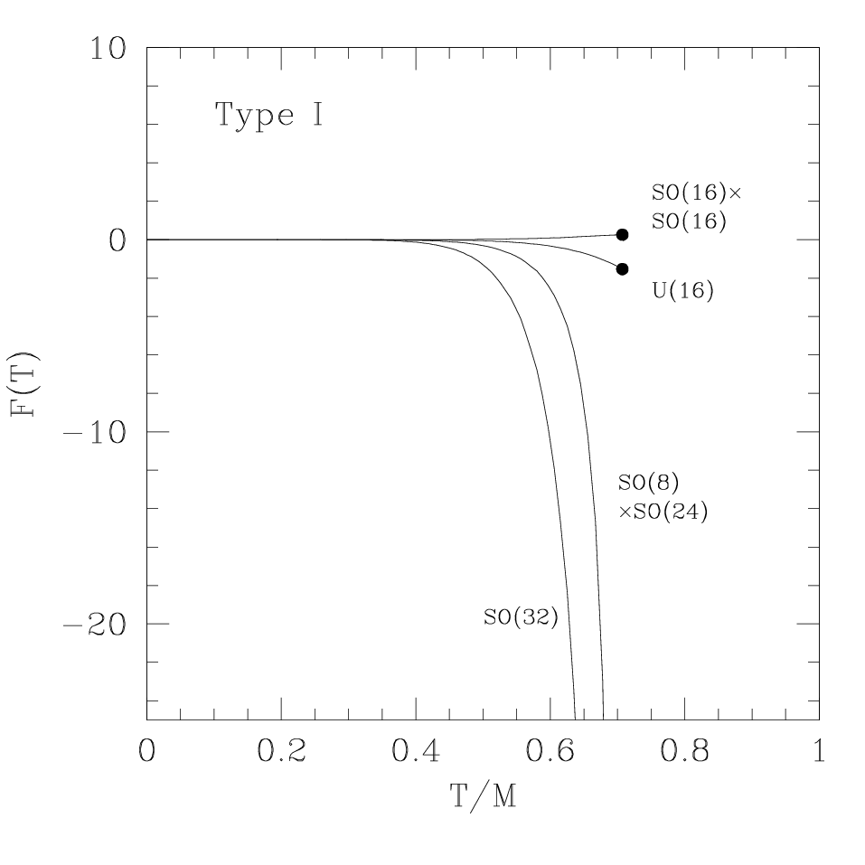
Given the set of Wilson lines outlined above, we can now examine their corresponding free energies . As discussed in Sect. II, for Type I string models the corresponding free-energy density receives separate contributions from the torus, the Klein bottle, the cylinder, and the Möbius amplitudes; these are shown in Eqs. (20), (21), and (22). In particular, several particular Wilson lines will interest us, such as those which yield the gauge groups we have considered for heterotic strings:
| (63) |
The results are shown in Fig. 3. Note that several of these results have also appeared in a different context in Ref. [16].
It is straightforward to understand the general features shown in Fig. 3. First, we recall from the above discussion that all four of these possible finite-temperature extensions share the same torus and Klein-bottle contributions to the free-energy density: as shown in Fig. 3(a), the torus contribution is relatively small and negative for , remaining finite until it diverges discontinuously at the critical temperature , while the Klein-bottle contribution actually vanishes as a result of the identity which holds for the characters of the transverse Lorentz group. Thus, as expected, it is the cylinder and Möbius contributions which are responsible for the relative differences between these different Wilson-line choices.
Let us first consider the Wilson-line cases following from the choice in Eq. (58). As indicated above, these cases all share the same Möbius contribution as well. Like the torus contribution, the Möbius contribution is also relatively small for ; however, unlike the torus contribution, we see from Fig. 3(a) that it is positive rather than negative and does not diverge, even at . Indeed, if these were the only three contributions in the Wilson-line cases, we would obtain the total curve which is shown in Fig. 3(b) for . In this case, the discontinuous divergence at is solely due to the closed-string tachyon coming from the torus amplitude in Fig. 3(a). However, for all other cases with , we also have a relatively huge cylinder contribution which is negative for , with smoothly as . In fact, recalling the character identity , we see from Eq. (60) that the overall general magnitude of this contribution is proportional to
| (64) |
Thus the case (i.e., the case with vanishing Wilson line) has the most negative cylinder contribution and correspondingly the most negative total free-energy density from amongst the choices with gauge groups .
Of course, it still remains possible that the case in Eq. (61) might yield a free-energy density which is even more negative. However, since when , we see that the cylinder contribution in Eq. (62) actually vanishes for this case. The Möbius contribution remains small but switches sign, becoming negative, but it continues to remain finite, even at . [Indeed, as discussed above, only in the and cases are all open-string tachyons avoided.] As a result, the free-energy density in the case remains small, diverging discontinuously at only because of the closed-string tachyon in the torus amplitude.
Comparing Fig. 3 for the Type I string with the analogous plot for the heterotic string in Fig. 2, we see certain superficial similarities. For example, the set of permitted gauge groups is similar in each case, and moreover Wilson-line choice in each case that leads to the minimum free energy is the one that breaks the gauge group minimally. However, we stress that despite such superficial similarities, there remains one fundamental distinction between the heterotic and Type I cases: except for the cases involving the particular and Wilson lines, the Type I cases lead to free-energy densities which actually diverge smoothly as the Hagedorn temperature is approached, i.e., as , while the corresponding heterotic free-energy densities actually remain finite as . This feature is already well known in the string-thermodynamics literature: it is a direct result of the open-string tachyon at , and suggests that the Hagedorn temperature is actually a limiting temperature for Type I strings rather than the location of a phase transition.
V Wilson lines and the Hagedorn temperature
As we have seen, one of the most prominent aspects of thermal string theories is the existence of a Hagedorn transition at which the string free-energy density diverges. However, the introduction of a non-trivial Wilson line can actually change the temperature at which this transition takes place. This is particularly true for heterotic strings, and we have already seen evidence of this fact in Fig. 2: the free-energy densities corresponding to the different possible Wilson-line choices all diverge at critical temperatures which differ from the Hagedorn temperature normally associated with the heterotic string without Wilson lines.
In some sense, it is to be expected that the introduction of non-trivial Wilson lines can affect the resulting Hagedorn temperature, since we have seen that such Wilson lines affect the thermal partition function as a whole. However, we can equivalently associate the Hagedorn temperature with the asymptotic densities of bosonic and fermionic states in the original zero-temperature theory, and the zero-temperature theory is clearly independent of the introduction of a non-trivial thermal Wilson line. Our goal in this section is to explain these different perspectives, and to show how they can ultimately be reconciled with each other in the presence of a non-trivial Wilson line. For concreteness, we shall focus on the case of the and heterotic strings, and examine the consequences of moving from the standard thermal theories in Eq. (15) which do not involve non-trivial Wilson lines to the new thermal theories [such as those in Eqs. (46) through (49) for , and those in Eqs. (52) through (55) for ] which do.
V.1 The Hagedorn transition: UV versus IR
We begin with several preliminary remarks concerning the Hagedorn transition and its dual UV/IR nature.
The Hagedorn transition is one of the central hallmarks of string thermodynamics. Originally encountered in the 1960’s through studies of hadronic resonances and the so-called “statistical bootstrap” [20, 21, 22], the Hagedorn transition is now understood to be a generic feature of any theory exhibiting a density of states which rises exponentially as a function of mass. In string theory, the number of states of a given total mass depends on the number of ways in which that mass can be partitioned amongst individual quantized mode contributions, leading to an exponentially rising density of states [1]. Thus, string theories should exhibit a Hagedorn transition [23, 24, 3, 7, 25]. Originally, it was assumed that the Hagedorn temperature is a limiting temperature at which the internal energy of the system diverges. However, later studies demonstrated that for closed strings the internal energy actually remains finite at this temperature. This then suggests that the Hagedorn temperature is merely the critical temperature corresponding to a first- or second-order phase transition.
There has been much speculation concerning possible interpretations of this phase transition, including a breakdown of the string worldsheet into vortices [24] or a transition to a single long-string phase [25]. It has also been speculated that there is a dramatic loss of degrees of freedom at high temperatures [7]. Over the past two decades, studies of the Hagedorn transition have reached across the entire spectrum of modern string-theory research, including open strings and D-branes, strings with non-trivial spacetime geometries (including AdS backgrounds and -waves), strings in magnetic fields, strings, tensionless strings, non-critical strings, two-dimensional strings, little strings, matrix models, non-commutative theories, as well as possible cosmological implications and implications for the brane world. A brief selection of papers in many of these areas appears in Refs. [8, 26, 27, 28, 29, 30, 31, 32, 33, 34, 35, 36, 37, 38].
In general, determining the Hagedorn temperature associated with a given finite-temperature thermal partition function is relatively straightforward. Given this thermal partition function, the one-loop free-energy density is given by the modular integral in Eq. (8), whereupon the full panoply of thermodynamic quantities such as the internal energy , entropy , and specific heat then follow from the standard definitions , , and . In string theory, the Hagedorn transition is usually associated with a divergence or other discontinuity in the free energy as a function of temperature. It turns out that are only two ways in which such a divergence may arise within the expression in Eq. (8).
First, of course, is the possibility of a divergence or discontinuity due to the well-known exponential rise in the degeneracy of string states which contribute to . This may be considered an ultraviolet (UV) divergence because it is triggered by the behavior of the extremely massive portion of the string spectrum. However, it turns out that this rise in the state degeneracies ultimately does not cause to diverge. To understand why, we may expand in the form where , where describe the right- and left-moving worldsheet energies (with thermal contributions included), and where describe the corresponding degeneracies of bosonic minus fermionic states. Although the degeneracies indeed experience exponential growth of the generic form where are positive coefficients, the contribution of each such state to the modular integrand in Eq. (8) is suppressed according to . For all and sufficiently large , this exponential suppression easily overwhelms the exponential rise in the degeneracy of states. As a result, the integrand in Eq. (8) remains convergent everywhere except as . However, this dangerous UV region is explicitly excised from the fundamental domain in Eq. (3). Thus, we conclude that the expression in Eq. (8) does not suffer from any UV divergences resulting from the exponential growth in the asymptotic degeneracies of states.
On the other hand, the expression in Eq. (8) may experience a divergence due to on-shell states within which may become massless or tachyonic at specific critical temperatures. For example, as the temperature increases, there may exist a critical temperature at which certain states which were massive for become massless at and ultimately tachyonic for . This can therefore be considered an infrared (IR) divergence. Since such on-shell tachyons correspond to states with worldsheet energies , their contributions to the modular integral in Eq. (8) grow as . The contributions from the (infrared) region of the fundamental domain then lead to a divergence for .
Thus, a study of the Hagedorn transition in string theory essentially reduces to a study of the tachyonic structure of as a function of temperature. Before proceeding further, however, we caution that we have reached this conclusion only because we have chosen to work in the so-called -representation for given in Eq. (8). By contrast, utilizing Poisson resummations and modular transformations [3], we can always rewrite as the integration of a different integrand over the strip
| (65) |
In such an -representation, the IR divergence as is transformed into a UV divergence as . This formulation thus has the advantage of relating the Hagedorn transformation directly to a UV phenomenon such as the exponential rise in the degeneracy of states. However, both formulations are mathematically equivalent; indeed, modular invariance provides a tight relation between the tachyonic structure of a given partition function and the rate of exponential growth in its asymptotic degeneracy of states [39, 40, 41, 42]. In the following, therefore, we shall utilize the -representation for and focus on only the tachyonic structure of , but we shall comment on the connection to the asymptotic degeneracy of states in Sect. V.C.
V.2 Effect of Wilson lines on Hagedorn temperature
So what then are the potential tachyonic states within , and at what temperatures do they first arise? Note that we are concerned with states whose masses are temperature-dependent: positive at temperatures below a certain critical temperature, zero at the critical temperature, and tachyonic at temperatures immediately above the critical temperature. The sudden appearance of such new “thermally massless” states at a critical temperature is the signal of the appearance of the long-range order normally associated with a phase transition, and the fact that such states generally become tachyonic immediately above reflects the instabilities which are also normally associated with a phase transition.
As a result, in order to derive the Hagedorn temperature of a given theory, it is sufficient to search for states within the thermal partition function whose masses decrease as a function of temperature, reaching (and perhaps even crossing) zero at a certain critical temperature. We shall refer to such states as “thermally massless” at the critical temperature. Since thermal effects always provide a positive contribution to the squared masses of any states, such states must intrinsically be tachyonic at zero temperature. In other words, for such thermally massless states, masslessness is achieved at the critical temperature as the result of a balance between a tachyonic non-thermal mass contribution (arising from the characters within ) and an additional positive temperature-dependent thermal mass contribution (arising from the thermal functions).
We can quantify this mathematically as follows. A given state with worldsheet energies will contribute a term of the form to the characters within . Likewise, as evident from their definitions in the Appendix, the thermal functions will make an additional, thermal contribution to these energies which is given by
| (66) |
where are respectively the momentum and winding quantum numbers around the thermal circle and where . The conditions for thermal masslessness then become
| (67) |
which together imply the useful relation . Since the thermal contributions in Eq. (66) are strictly non-negative (and are not zero, according to our assumption of thermal masslessness), we see that the possibility of obtaining a thermally massless state requires that either or (or both) must be negative, and neither can be positive. In other words, the zero-temperature state contributing within the characters within must be a tachyon which is either on-shell (if ) or off-shell (if ); this tachyonic mode is then “dressed” with specific thermal contributions in order to become massless at the critical temperature . Moreover, if our solution to Eq. (67) has non-zero , then such a state will be massive for all temperatures below this critical temperature, as desired. It will also usually be tachyonic for temperatures immediately above this critical temperature.
Given these observations, our procedure for determining the Hagedorn temperature corresponding to a given thermal partition function is then fairly straightforward. First, we identify any zero-temperature states which are tachyonic (either on- or off-shell) contributing to the characters appearing within . For each such state, we then attempt to solve the conditions in Eq. (67), subject to the constraints that are restricted to the values which are appropriate for the corresponding thermal function (i.e., or and or ). If such a solution exists and has non-zero , then we have succeeded in identifying a massive state in the full thermal theory which will become massless at the corresponding critical temperature . This then signals a Hagedorn transition. In situations where multiple thermally massless states exist, the Hagedorn temperature is identified as the lowest of the corresponding critical temperatures, since the presumed existence of a phase transition at that temperature invalidates any analysis based on at temperatures above it.
Let us now calculate the Hagedorn temperatures corresponding to the heterotic partition functions in Sect. IV. We focus first on the standard heterotic results without Wilson lines, as given in Eq. (15). For both the and cases, we find that the sector is the sector which is capable of providing thermally massless states at the lowest possible temperature. Indeed, solving the conditions for masslessness in Eq. (67), we see that the off-shell tachyon within — dressed with the thermal excitations within — becomes thermally massless at the critical temperature . This, of course, is nothing but the traditional Hagedorn temperature associated with the and heterotic strings.
By contrast, let us now examine the thermal partition functions for the string which are constructed using non-trivial Wilson lines. For example, if we concentrate on the partition function in Eq. (46), we now find that the term is the one which gives rise to thermally massless level-matched states at the lowest possible temperature. Indeed, the character gives rise to 32 on-shell tachyons, and these are nothing but the 32 tachyons of the non-supersymmetric heterotic string which serves as the endpoint of the corresponding Wilson-line orbifold. Moreover, we find that the thermal excitations of these states are massless at , massive below this temperature, and tachyonic above it. Indeed, there are no other tachyonic sectors within Eq. (46) which could give rise to other phase transitions at lower temperatures. Thus the Hagedorn temperature associated with Eq. (46) is actually given by , not , and agrees with the locations of the divergences indicated in Fig. 2. Remarkably, this new temperature is exactly the same as the Hagedorn temperature of the Type I and Type II strings.
The same is true for Eqs. (47) and (48) as well: each of these thermal partition functions corresponds to , not . This makes sense, since each of these Wilson lines corresponds to a non-supersymmetric heterotic model containing on-shell tachyons with worldsheet energies . Indeed, the only exception is the partition function in Eq. (49). This too makes sense, since the Wilson line in this case corresponds the heterotic string model. Although non-supersymmetric, this string model is tachyon-free. Indeed, for the partition function given in Eq. (49), we find that off-shell tachyons with arise within the term ; these, when dressed with the thermal excitations within , become massless at . This is the lowest temperature at which such thermally massless states appear, which identifies this as the Hagedorn temperature corresponding to the Wilson line.
A similar situation exists for the possible thermal extensions of the string. Examining Eq. (52), we see that only the sector is capable of giving rise to thermally massless level-matched states; once again, these are the tachyons with energies within , dressed with the thermal excitations within . These states are massless at , massive below this temperature, and tachyonic above it. Thus, we see that emerges as the Hagedorn temperature following from Eq. (52) as well. Indeed, the same is also true for Eqs. (53) and (54), while we find that for Eq. (55). These results are precisely in one-to-one correspondence with those for the string.
We conclude, then, that the existence of non-trivial Wilson lines in the formulation of finite-temperature heterotic strings has, in most cases, shifted the corresponding heterotic Hagedorn temperature from to . Remarkably, this is the same Hagedorn temperature as that associated with Type II strings. It is easy to understand why this is the case. Without a non-trivial Wilson line, our thermal heterotic theories are described by Eq. (15), and the lowest mode contributing within is the (tachyonic) ground state of the heterotic theory, with non-level-matched vacuum energies . However, as we have seen, turning on the Wilson lines leading to Eqs. (46), (47), and (48) in the case, or to Eqs. (52), (53), and (54) in the case, effectively projects this non-level-matched state out of the finite-temperature theory and leaves behind only the “next-deepest” tachyon with within . Thus, with these Wilson lines turned on, this new tachyon becomes the effective ground state of the theory. However, this “next-deepest” tachyon has exactly the same worldsheet energies as the ground state of the Type II string. Thus it is not surprising that the presence of the non-trivial Wilson line shifts the corresponding heterotic Hagedorn temperature in such a way that it now matches the Type II value.
V.3 Reconciling the shifted Hagedorn temperature with the asymptotic degeneracies of states
As discussed in Sect. V.A, our analysis of the Hagedorn temperature has thus far been based on an analysis of the tachyonic structure of our thermal partition functions. Yet we know that there is a tight relation between the Hagedorn temperature of a given theory and the exponential rate of growth of its asymptotic degeneracies of bosonic and fermionic states. Specifically, if denotes the number of string states with mass , then the thermal partition function is given by . However, if as , then diverges for . This appears to provide a firm link between the Hagedorn temperature and the asymptotic degeneracy of states. Of course, is not a proper string-theoretic partition function. However, even when we utilize a proper string-theoretic partition function and calculate a proper string-theoretic amplitude as in Eq. (3) in the -representation, the same basic argument continues to apply.
We are thus left with the critical question: How can we justify a shifted Hagedorn temperature for heterotic strings, given that the zero-temperature bosonic and fermionic densities of heterotic states are apparently unchanged? This question is particularly urgent, given that the feature which is inducing this shift in the Hagedorn temperature — namely the introduction of a non-trivial thermal Wilson line — does not affect the zero-temperature theory in any way. Specifically, an increase in the Hagedorn temperature of the heterotic string from the traditional value to a new, higher value would seem to require a corresponding decrease in the exponential rate of growth of the asymptotic density of heterotic string states. In what sense can we understand such a decrease?
To answer this question, let us look again at the original partition function of the zero-temperature ten-dimensional heterotic string model in Eq. (43). Recall that and indicate the transverse Lorentz spins of the different states which contribute in this theory. As a result of spacetime supersymmetry, this partition function vanishes identically — i.e., all of its level-degeneracy coefficients are identically zero. There is no exponential growth here at all. But of course one does not examine the total partition function in order to derive a Hagedorn temperature; one instead looks at its separate bosonic and fermionic contributions. Ordinarily, these contributions would be identified on the basis of the Lorentz spins of these states as
| (68) |
and indeed each of these expressions separately exhibits an exponential rise in the degeneracy of states which is consistent with the traditional heterotic Hagedorn temperature.
But what do we really mean by “bosonic” and “fermionic” in this context? For most purposes, we would identify states as “bosonic” or “fermionic” based on their Lorentz spins, as above. Moreover, by the spin-statistics theorem, this is equivalent to identifying states as bosonic or fermionic based on their zero-temperature quantization statistics. However, for the purposes of computing a Hagedorn temperature, we should really be focused on a thermodynamic definition of “bosonic” and “fermionic” wherein we identify states as bosons or fermions on the basis of their Matsubara frequencies, i.e., on the basis of their modings around the thermal circle. Of course, under normal circumstances, all three of these identifications are equivalent. However, we have already seen in Sect. III that this chain of equivalences is modified in the presence of a non-trivial Wilson line: certain states which are “bosonic” in terms of their Lorentz spins and zero-temperature quantization statistics can nevertheless have half-integer modings around the thermal circle, while other states which are “fermionic” in terms of their Lorentz spins and zero-temperature quantization statistics can nevertheless have integer modings around the thermal circle. Thus, in the presence of a non-trivial Wilson line, certain bosonic states can behave as fermions from a thermodynamic standpoint, and certain fermionic states can behave as bosons.
We emphasize that this is not a violation of the spin-statistics theorem. Indeed, the spin-statistics theorem is believed to hold without alteration in string theory, providing a connection between the Lorentz spin of a state and its zero-temperature quantization statistics [1]. Rather, as discussed in Sect. III, the effect of the Wilson line is to modify the thermodynamic manifestation of these properties as far as their Matsubara modings are concerned. For issues pertaining to zero-temperature physics, these thermodynamic manifestations may be of little consequence. However, when we seek to understand the thermal properties of a theory, these modifications are critical.
Therefore, if we seek to understand the spectra of bosonic and fermionic states in the heterotic string for thermodynamic purposes, we should return to the partition function in Eq. (43) and separate this expression into individual contributions from bosonic and fermionic states on the basis of their Matsubara modings around the thermal circle. It is here where the Wilson line comes into play.
Let us begin by considering the case of the string. Without a Wilson line, we know that bosonic states will correspond to integer Matsubara modings and fermionic states will correspond to half-integer modings . This corresponds to the traditional identifications in Eq. (68), and these lead to the traditional Hagedorn temperature .
However, under the influence a non-trivial Wilson line, these identifications can change. For example, let us consider the case of the Wilson line corresponding to Eq. (46). In this case, the “bosonic” contributions to Eq. (43) must be identified as those which multiply the thermal sum in Eq. (46), while the “fermionic” contributions to Eq. (43) must be identified as those which multiply the thermal sum in Eq. (46). In other words, we replace the identifications in Eq. (68) with
| (69) |
In the presence of the non-trivial Wilson line, it is therefore these expressions which serve to define our separate bosonic and fermionic contributions to Eq. (43), and indeed their sum
| (70) |
correctly reproduces the expression in Eq. (43).
Given these results, we can now calculate the exponential rates of growth in the degeneracies of the states contributing to and in Eq. (69). We find that while each individual term within and in Eq. (69) continues to exhibit the traditional rate of growth associated with the traditional Hagedorn temperature for heterotic strings, the minus signs within and have the net effect of cancelling this dominant exponential behavior, leaving behind only a smaller exponential rate of growth for the state degeneracies corresponding to and . Moreover, as expected, this smaller exponential rate of growth precisely matches the rate of growth that corresponds to the new (increased) heterotic Hagedorn temperature . Similar results also hold the Wilson lines associated with Eqs. (47) and (48).
It may seem strange that two terms, each exhibiting a dominant exponential growth rate, can be subtracted and leave behind a sub-dominant exponential growth rate. Yet this phenomenon is well known for modular functions such as these, and has been shown to operate in other string-theoretic contexts [39, 40, 41, 43]. We emphasize that this subtraction is relevant only in the sense that it deforms the exponential growth rate when we count and separately. Each string state still continues to appear with positive unit weight in the string Fock space, as always, and still contributes to the overall partition function with unit weight and an appropriate sign (positive for spacetime bosons, negative for spacetime fermions).
Similar results hold for the heterotic string. Without a Wilson line, the usual identification of bosonic and fermionic states is nothing but
| (71) |
However, in the presence of the Wilson line associated with Eq. (52), we find that our new thermal identification of bosonic and fermionic states is given by
| (72) |
Just as with the string, the minus signs within Eq. (72) lead to state degeneracies which show a reduced exponential growth — one which is precisely in accordance with the new, increased heterotic Hagedorn temperature associated with this Wilson line. Similar results also hold the Wilson lines associated with Eqs. (53) and (54).
This, then, is the essence of the manner in which the asymptotic density of states is ultimately reconciled with the modified Hagedorn temperature for heterotic strings. The presence of the non-trivial Wilson line “deforms” the thermal identification of bosonic and fermionic states, trading states between the separate sets of bosonic and fermionic states in such a way that the net exponential rate of growth for the asymptotic state degeneracy of each set is reduced.
There are also other ways to understand this result. For example, one might argue on general conformal-field-theory (CFT) grounds that such a change in the Hagedorn temperature should not be possible. After all, there exists a general result which relates the Hagedorn temperature of a given closed-string theory to the central charges of its underlying worldsheet CFT’s:
| (73) |
For Type II strings, we have , while for heterotic strings, we have . However, in deriving Eq. (73), there is only place in which the central charges enter: this is in setting the ground-state energies . Moreover, as we have seen in Sect. V.B, the Wilson line has effectively projected the true heterotic ground state with out of the spectrum, leaving behind only the “next-deepest” tachyon with to serve as the effective ground state of the theory. Thus, in the presence of the Wilson line, the effective central charges of the theory become , just as for Type II strings.
We see, then, that the introduction of a non-trivial Wilson line induces both a shift in the vacuum energy of the effective ground state and a shift in the asymptotic rates of growth for the state degeneracies. These shifts, of course, are flip sides of the same coin, deeply related to each other through modular transformations. Indeed, these are nothing but equivalent UV/IR descriptions of the same phenomenon, all arising due to the existence of the non-trivial Wilson line. Under Poisson resummation, a half-integer shift in the moding of a given set of string states around the thermal circle translates into an overall phase (i.e., a minus sign) in front of the corresponding character in the partition function. Thus the Wilson line, which shifts the apparent thermal modings of certain states in the theory, necessarily induces a corresponding change in the asymptotic state degeneracies and a corresponding shift in the Hagedorn temperature of the theory.
We thus conclude that the introduction of a non-trivial Wilson line has the potential to change the Hagedorn temperature of the resulting thermal theory, and in many cases actually shifts this temperature from its traditional heterotic value to a new value which is the same as that associated with Type I and Type II strings. Indeed, although the heterotic string would naïvely appear to have a slightly lower Hagedorn temperature than the Type II string due to its non-level-matched ground state, we see that the introduction of a non-trivial Wilson line has the potential to eliminate this discrepancy. Such Wilson lines deform the effective worldsheet central charges of the heterotic theory as far as its thermal properties are concerned, and lead to new, effective ground states for the theory as well as modified rates of exponential growth for the corresponding bosonic and fermionic densities of states. Both effects then alter Hagedorn temperature of the heterotic string, and potentially bring it into agreement with the Type I and Type II value.
V.4 The “spectrum” of Hagedorn temperatures: A general classification
As we have seen in Sect. V.B, the thermal heterotic theories without Wilson lines have the Hagedorn temperature ; indeed, this is the case because the relevant partition functions in Eq. (15) each contain a term of the form . Indeed, such a term encapsulates the contribution of the tachyon, and this is the state which, when dressed with the thermal excitations within , is massive at low temperatures but becomes massless at .
By contrast, we found that this state is projected out of the thermal partition function when non-trivial Wilson lines are introduced. For example, for the Wilson lines leading to Eqs. (46) and (52), we found that the “next-deepest” remaining tachyons have worldsheet energies ; indeed, these are the tachyons which contribute to the terms which appear within Eqs. (46) and (52). These tachyons, when dressed with the thermal excitations within , are massless at , massive below this temperature, and tachyonic above it. Thus, emerges as the Hagedorn temperature corresponding to these choices of Wilson lines. We found that this result also holds for the Wilson lines leading to Eqs. (47), (48), (53), and (54). By contrast, we found that the Hagedorn temperature is for the Wilson lines leading to Eqs. (49) and (55). Indeed, in these cases, even the tachyons are projected out of the spectrum, so that the lowest possible remaining tachyons have and contribute to the sector.
Given these results, it is natural to wonder whether other Hagedorn temperatures might also be possible. Indeed, one might even wonder whether there exist Wilson lines for which the Hagedorn transition might be avoided completely! Of course, neither of these options is possible for the supersymmetric heterotic strings in ten dimensions, for we have presented a complete classification of all self-consistent Wilson lines in such cases, and our results are quoted above. However, in lower dimensions, this might no longer be the case. In fact, in lower dimensions, even the Type II superstrings can have non-trivial Wilson lines which are associated with the gauge symmetries that emerge upon compactification. Thus, these questions become relevant for Type II strings as well as heterotic.
Towards this end, we shall now provide a general classification all of the Hagedorn temperatures which can ever be realized for closed strings with non-trivial Wilson lines. Our analysis will apply to all closed strings, both Type II and heterotic.
For concreteness, we shall restrict our attention to theories built from only orbifolds, so that are quantized in half-integer values. Given the heterotic constraints and (which also subsume the Type II constraints ), we then find that there are only eight different terms which could possibly appear in and trigger a Hagedorn transition. These are listed in Table 1, along with their corresponding thermal excitations and Hagedorn temperatures [obtained by solving Eq. (67)]. It is interesting to note the mathematical fact that these terms come in “dual” pairs under which and . Roughly speaking, this duality corresponds to exchanging the direction of the corresponding “interpolating” thermal partition functions, exchanging the and endpoints. Although this “thermal duality” phenomenon has played a significant role in other work [3, 6, 7, 1, 44, 45]), it will not be critical for the following discussion. We can therefore view the emergence of this duality within Table 1 as a mere mathematical curiosity.
| Thermal Function | Thermal Modes | ||||
|---|---|---|---|---|---|
| A | |||||
| (also ) | |||||
| B | , | ||||
| , | |||||
| C | , | ||||
| D | , | ||||
| E | |||||
| F | |||||
| G | |||||
| H |
As we have already seen, Case A is responsible for the traditional heterotic Hagedorn transition and leads to the lowest possible Hagdorn temperature . Likewise, Case C with is responsible for the traditional Type II Hagedorn transition as well as the shifted heterotic Hagedorn transitions with . Indeed, this case produces what is ultimately the “next-lowest” Hagedorn temperature, and as such it dominates [when present within ] over any other terms which may also simultaneously appear within . Indeed, in ten dimensions, our complete enumeration of all possible non-trivial Wilson lines in the heterotic case has demonstrated that Case C with arises in all but cases. By contrast, the Wilson lines are examples of Case F.
Ultimately, the question of which of these terms ends up dominating for a given string model in dimensions is likely to be addressable only on a case-by-case basis. Nevertheless, it is easy to see that Cases B and D can only arise for string models which are already tachyonic (and hence unstable) at zero temperature; this follows from the fact that the solutions for their corresponding Hagedorn temperatures, as shown in Table 1, always include the cases with or . This can also be seen by taking the direct limit of the terms in each of these cases. Thus, Cases B and D need not concern us further.
Given this situation, it is natural to wonder whether there are any Wilson-line choices for which the Hagedorn transition is eliminated completely — i.e., string models in which no thermally massless states appear at any temperature, and in which none of the remaining cases listed in Table 1 arise. However, we shall now prove that this cannot happen for any heterotic string which is supersymmetric at zero temperature, regardless of its spacetime dimension. In particular, we shall demonstrate that Case H will always arise for such strings, giving rise to a Hagedorn transition at if no earlier Hagedorn transition has occurred at lower temperature.
Our argument is completely general since it is based on considerations of the most generic massless states in the perturbative heterotic string: those associated with the gravity multiplet. Recall that in the heterotic string, the graviton is realized in the Neveu-Schwarz sector as
| (74) |
where and are respectively the excitations of the right-moving worldsheet Neveu-Schwarz fermion and left-moving worldsheet coordinate boson . Since the Neveu-Schwarz heterotic-string ground state has vacuum energies , the states in Eq. (74) are both level-matched and massless, with . These states include the spin-two graviton, the spin-one antisymmetric tensor field, and the spin-zero dilaton.
In a similar vein, any model exhibiting spacetime supersymmetry must also contain the gravitino state, realized in the Ramond sector of the heterotic string as
| (75) |
Here schematically indicates the Ramond zero-mode combinations which collectively give rise to the spacetime Lorentz spinor index , as required for the spin-3/2 gravitino state.
Regardless of the particular GSO projections inherent in the particular string model under consideration, we know that the graviton state in Eq. (74) must always appear in the string spectrum. Likewise, if the model has spacetime supersymmetry, we know that the gravitino state in Eq. (75) must exist as well. However, it is then straightforward to show that this implies that certain additional off-shell tachyons must also exist in the string spectrum. Specifically, regardless of the particular GSO projections, the off-shell spectrum will always contain a spin-one “proto-graviton” state in the Neveu-Schwarz sector:
| (76) |
likewise, if the model is spacetime supersymmetric, the off-shell spectrum will always contain a spin-1/2 “proto-gravitino” state in the Ramond sector:
| (77) |
Note that these are the same states as the graviton/gravitino, except that in each case the left-moving bosonic excitation is lacking. However, it is important to realize that GSO projections are completely insensitive to the presence or absence of excitations of the worldsheet coordinate bosonic fields. This is indeed a general property of GSO projections. Thus, since the graviton is always present in the on-shell spectrum, it then follows that the proto-graviton must also always be present in the off-shell spectrum; likewise, if the model is supersymmetric and the gravitino is present in the on-shell spectrum, then the proto-gravitino must also always be present in the off-shell spectrum. Thus, we conclude that the proto-graviton and proto-gravitino are two off-shell tachyons with worldsheet energies which generically appear in all supersymmetric heterotic string models.
This does not, in and of itself, guarantee that these states will contribute to the thermal partition function within the specific or sectors that Cases G or H would require. Fortunately, however, it is not too difficult to determine which sectors will contain these states. Like the graviton and gravitino states from which they are derived, these proto-graviton and proto-gravitino states must exist in the zero-temperature theory and thus must survive the zero-temperature limit. This implies that these states must appear in the sectors, not the sectors. Moreover, since neither of these states carries any gauge charges, neither can be affected by the presence of a Wilson line. As a result, we know that the (bosonic) proto-graviton state must appear in the sector (which has integer modings around the thermal circle), while the (fermionic) proto-gravitino state must appear in the sector (which has half-integer modings).
Given these results, we conclude that while the proto-graviton state will never lead to any of the cases in Table 1, the proto-gravitino state leads directly to Case H. Moreover, as we have argued on general grounds, this state is always present in any heterotic model which is supersymmetric at zero temperature. As a result, we conclude that the proto-gravitino state — dressed with thermal excitations — will always exist and trigger a Hagedorn-like transition at temperature (provided no other phase transition has occurred at any lower temperature).
This transition is somewhat different from the typical Hagedorn transition, however. In general, the total spacetime mass of a given state dressed with thermal excitations varies with the temperature according to
| (78) |
where . However, for the proto-gravitino (Case H), this becomes
| (79) |
whereupon we see that the thermal excitation of the proto-gravitino state never becomes tachyonic! Indeed, this state is massive for all , and merely hits masslessness at before becoming massive again at higher temperatures. Of course, this result is completely consistent with the fact that the proto-gravitino state is fermionic, since the existence of a physical fermionic tachyon at any temperature would violate Lorentz invariance.
However, given that this state never becomes tachyonic, it is natural to wonder whether this state can ever give rise to a Hagedorn transition. Indeed, since no tachyon ever develops, the free-energy density will never diverge. To study this issue, let us define the vacuum amplitude , whereupon we observe that the thermal excitation of the proto-gravitino state makes a contribution to given by
| (80) | |||||
where we have left the temperature arbitrary. Note that the leading factor in the first line of Eq. (80) represents the zero-temperature contribution from the proto-gravitino, with , while the remaining factor in brackets represents the thermal contribution with . Likewise, we have carefully recorded all factors of : two factors of arise in the denominator from the modular-invariant measure of integration, factors arise in the numerator from the zero-temperature partition function, and an additional factor arises in the numerator from the definitions of the thermal sums. However, at , this expression reduces to
| (81) |
and as , this contribution scales like
| (82) |
This contribution is therefore finite for all . This, of course, agrees with our usual expectation that a massless state does not lead to a divergent vacuum amplitude in two or more spacetime dimensions.
It is important to realize that even though remains finite for all temperatures, a phase transition still occurs; indeed the sudden appearance of a new massless state at a critical temperature signals the appearance of a new long-range order that was not present previously. Therefore, in order to elucidate the effects of this massless state, let us now investigate temperature derivatives of . As evident from the second line of Eq. (80), each temperature derivative brings down an extra factor of . In general, this thereby increases the tendency towards divergence of our thermodynamic quantities.
Our results are as follows. The contribution of this thermally excited proto-gravitino state to the first derivative is given by
| (83) |
but at the temperature we see that the factor in parentheses within Eq. (83) actually vanishes:
| (84) |
It turns out that this is a general property, reflecting nothing more than the fact that the slope of the mass function in Eq. (79) vanishes at its minimum, as it must. However, taking subsequent derivatives and evaluating at , we find the general pattern
| (85) |
where for is a rank- polynomial in of the form
| (86) |
where
| (87) |
and where the leading coefficients are positive for (mod 4) and negative for (mod 4), with alternating signs for the lower-order coefficients , , etc. Given these extra leading powers of , we thus find that as a result of the proto-gravitino state,
| (88) |
Equivalently, in spacetime dimensions, the proto-gravitino state results in a divergence that first occurs for , where
| (89) |
This divergence then corresponds to a very weak, -order phase transition. In particular, for , this would be a fourth-order phase transition in which diverges, causing to experience a discontinuity, the specific heat itself to experience a kink, and the internal energy function to have a discontinuous change in curvature. Similar kinds of phase transitions have also been discussed for two-dimensional heterotic strings in Ref. [38], and for Type I strings with non-trivial Wilson lines in Ref. [10]. These results for heterotic strings were first discussed in Ref. [46].
We stress that it is not merely the masslessness of this thermally-enhanced proto-gravitino state that results in this phase transition. It is the fact that this masslessness is achieved thermally, with non-trivial thermal momentum and winding quanta, that induces this phase transition. By contrast, a regular massless state such as the usual graviton or gravitino does not contribute to any temperature derivatives of .
Thus, we conclude that for supersymmetric heterotic strings, it is never possible to completely evade a Hagedorn-like phase transition. Indeed this result holds regardless of the specific Wilson line chosen when constructing the finite-temperature theory. However, the phase transition associated with the proto-gravitino state appears only at the relatively high temperature , and thus will be completely irrelevant if tachyon-induced Hagedorn transitions appear at lower temperatures.
VI A global thermal “landscape”: Stability and metastability for finite-temperature strings
Finally, in order to obtain a more global sense of the thermodynamic relations between different Wilson-line choices discussed in Sect. IV — and also in order to perform a more detailed comparison between the Type I and heterotic cases — we now enlarge our perspective and consider the general space of allowed Wilson lines for these thermal string theories. Our goal is to understand the behavior of the corresponding free energies of these theories as the underlying Wilson lines are allowed to vary. Note that in general, we could also consider the variation of a whole host of background fields and other moduli (such as the dilaton and temperature, or equivalently the thermal compactification radius); such analyses appear, e.g., in Refs. [47, 48]. Indeed, generic issues arising within this context are not only the dilaton-runaway problem but also a temperature-runaway problem (a stringy “greenhouse” effect!). However, for the purposes of our discussion, it will be sufficient to restrict our attention to those flat background gauge fields with vanishing field strengths — i.e., to the space of allowed Wilson lines in these thermal theories.
Such an analysis is also important for another reason. As we have discussed, our approach to generating the finite-temperature extension of a given zero-temperature string model is to treat these Wilson lines as free parameters that allow us to scan across all possible finite-temperature thermal partition functions, and to attempt to identify which Wilson line might lead to a minimum of the free energy with respect to variations of the Wilson line. Of course, in doing this we have tacitly been assuming that such a minimum is unique and is thus a global minimum. However, this need not be the case: such solutions might also correspond to local minima. In other words, adopting a terminology that suggests the possibility of “tunnelling” transitions between theories with different Wilson lines, we may refer to our preferred Wilson-line choice as leading to a thermal vacuum which is either thermodynamically stable or thermodynamically metastable within this sixteen-dimensional space. Resolving this issue therefore requires understanding something of the global structure of the free energy as a function of the possible Wilson-line choices.
VI.1 The thermal Type I landscape
In this section, it will prove simpler to begin by considering the case of the Type I string. We have already seen in Sect. IV that the , , , and cases correspond respectively to Wilson-line parameters given in Eq. (63). However, we now shall enlarge our discussion by considering each of the sixteen components of to be an independent general free parameter, and examine the free energy as a function over the resulting sixteen-dimensional parameter space , .
In general, it is relatively easy to calculate the general expressions that describe the Type I component partition functions as general functions of the sixteen parameters , . As we have discussed in Sect. IV, since the closed-string states are neutral with respect to the gauge group, their contributions to the total torus and Klein-bottle amplitudes are insensitive to the appearance of the Wilson line. As a consequence, the results for and in Eq. (27) remain valid even when a Wilson line is turned on. By contrast, as discussed above, the states contributing to the cylinder and Möbius partition functions carry gauge charges and consist of an anti-symmetric tensor (the adjoint representation) of the gauge group as well as a (reducible) symmetric tensor of the gauge group. If we denote by and the sets of gauge charges associated with these symmetric and anti-symmetric representations, respectively, we then find using the results in Eq. (41) that an arbitrary Wilson line parametrized by causes the thermal cylinder and Möbius partition functions in Eq. (27) to take the shifted forms [17, 49]:
It is straightforward to check that in the special case with , these expressions recombine to reproduce the results in Eq. (27), with the -dimensional symmetric representation of and the -dimensional anti-symmetric representation of adding and subtracting to produce the overall multiplicities and respectively.
Given the general expressions given in Eqs. (), we can now examine the corresponding free-energy thermal “landscape”. Performing this analysis is relatively straightforward. Setting to zero the first derivatives of these partition functions with respect to the 16 parameters gives us the critical points of this theory — note that this condition also ensures the consistency of the string vacuum in question by ensuring that all one-loop one-point functions vanish. Whether the extremum in question is a local maximum, minimum, or saddle point (or potentially even lying along a flat direction) can then be determined by examining the Hessian matrix of second derivatives.
Our results are not unexpected. As already anticipated, our thermodynamically preferred case corresponds to a local minimum which also turns out to be a global minimum. Thus this solution is thermodynamically stable. By contrast, each of the other cases listed in Eq. (63) is either a saddle point or local maximum. There are no metastable local (but not global) minima.
It proves instructive to consider a two-dimensional projection of this sixteen-dimensional parameter space. One such projection which distinctly captures all of the cases in Eq. (63) comes from restricting our attention to Wilson lines of the form
| (91) |
where and are taken to be our two free parameters, with and . In the T-dual theory, this Wilson line corresponds to having D8-branes coincident at the point on the thermal circle and the remaining D8-branes coincident with an orientifold fixed plane. In terms of these two parameters , the four cases in Eq. (63) are given by
| (92) |
Although is restricted to an integer, we will allow to range continuously within the range . Non-integer values of can be interpreted physically in the T-dual theory as effectively capturing the dynamics of a configuration with a total of 16 branes (and 16 image branes), some of which may be located at points other than and .

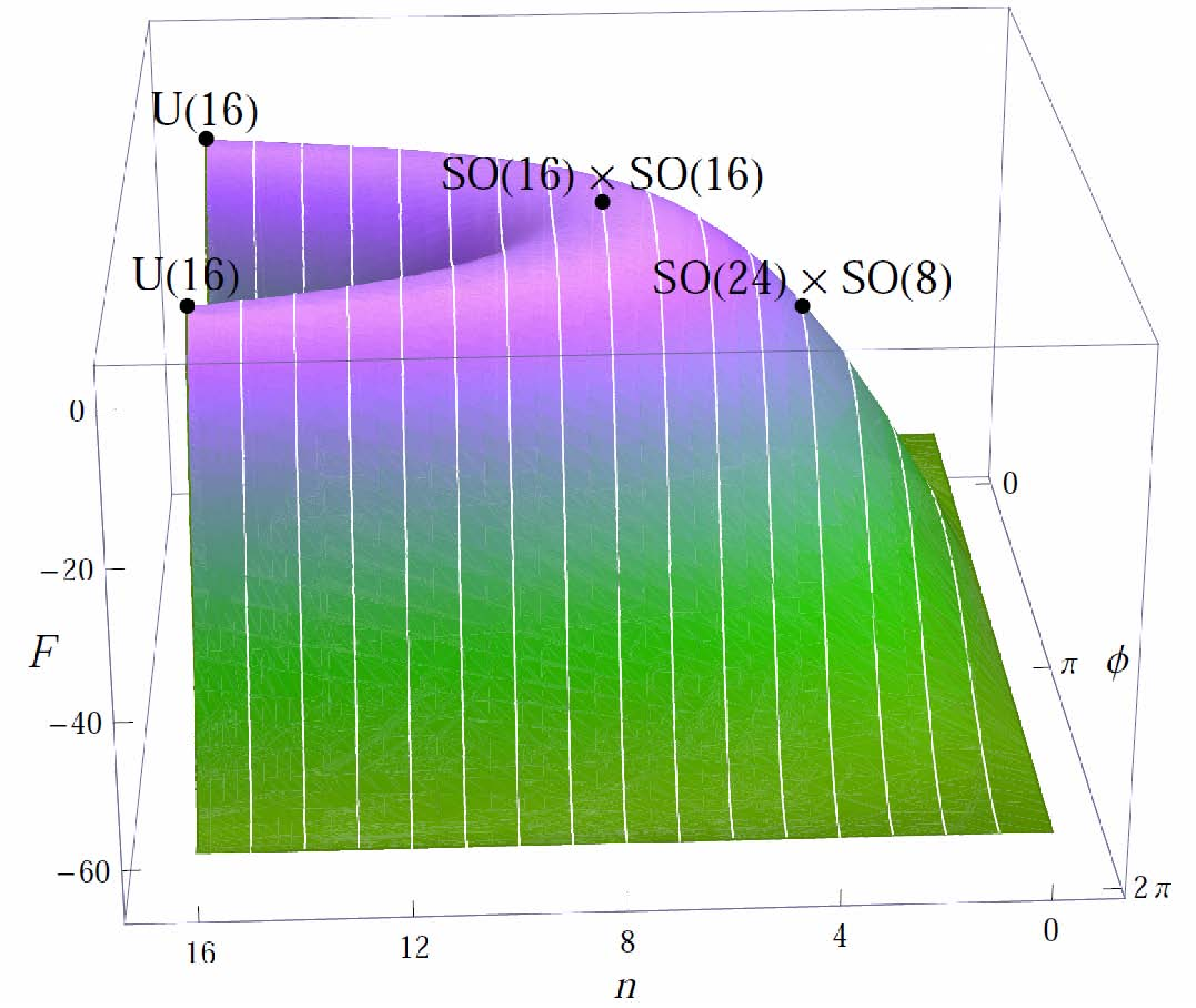
In Fig. 4 we plot the total Type I free-energy density as a function of and . As we see from Fig. 4, each of the cases we have examined in Eq. (92) appears as a critical point. Moreover, the non-SUSY theory appears as the global minimum. It is worth noting that the contour plot in Fig. 4 corresponds to a fixed reference temperature . As the temperature decreases, this contour becomes increasingly flat, becoming completely flat at (signalling the restoration of spacetime supersymmetry). On the other hand, as the temperature increases, the variations in this contour plot grow without bound, ultimately diverging as (signalling the approach to the Hagedorn transition).
It is also worth noting that this contour plot is periodic in the variable, with a periodicity of magnitude (or equivalently ). This periodicity arises because the perturbative Type I string contains states in only those “vectorial” representations (corresponding to the adjoint representation, the symmetric tensor, end the singlet) whose charges have integer coefficients. By contrast, if the perturbative Type I string had contained states in spinorial representations of (with charge vectors containing half-integer components), the periodicity of the resulting free-energy contour plot would have been twice as large, with . In such a case, we could expand the list of Wilson lines in Eq. (63), formally distinguishing two different classes of Wilson lines which preserve the gauge group of the Type I model:
| (93) |
The case with vanishing Wilson line is thus of type . Of course, since the perturbative Type I string does not contain spinorial states, both classes of Wilson lines lead to the same thermal Type I model.
VI.2 The thermal heterotic landscape
For the purpose of comparison, we now subject the ten-dimensional supersymmetric heterotic string to the same analysis.
The effects of Wilson lines on the thermal heterotic string are similar to the effects of Wilson lines on the thermal Type I string, with one notable exception: the fact that the heterotic string is closed implies that the thermal string spectrum contains not only momentum modes but also winding modes around the thermal circle. The effects of Wilson lines therefore affect both of these quantum numbers, as indicated in Eq. (42).
Given this, it is straightforward to generate the heterotic thermal partition functions which include the effects of generalized Wilson lines. To do this, we can begin with the thermal partition function corresponding to the special case with :
| (94) |
where the holomorphic functions are the characters associated with the gauge group. We can then use the results in Eq. (42) in order to incorporate the effects of a general Wilson line . To do this, we first recall from the Appendix that the and functions in Eq. (94) are given by double sums of the form given in Eq. (104), where the thermal momentum and winding numbers in the sum in Eq. (104) are restricted to the sets
| (95) |
Likewise, we recognize that
| (96) |
where is the Dedekind eta-function and where the lattice of weights associated with the character sum is given by
| (97) |
Given this, we then find that a general Wilson line deforms the expression in Eq. (94) to take the form
| (98) |
where
| (99) |
with . Indeed, the general expression in Eq. (98) is modular invariant for all values of and successfully reproduces the partition functions associated with each of the thermal heterotic interpolations discussed in Sect. IV for the specific Wilson-line choices listed in Eq. (50). Note, in particular, that the heterotic string contains states transforming in spinorial representations of (i.e., representations which have charge components ). As a result, the possible Wilson-line parameters must now be considered modulo 2 rather than modulo 1. As we shall discuss further below, this is an important distinction relative to the Type I case.
Despite the existence of the general expression in Eq. (98), it is important to bear in mind that not all Wilson lines correspond to self-consistent heterotic models. Indeed, as discussed in Sect. IV, only the explicit choices listed in Eq. (50) satisfy all necessary worldsheet constraints and lead to self-consistent heterotic models. We shall nevertheless consider the general unconstrained sixteen-dimensional parameter space of arbitrary Wilson-line choices in order to compare with the Type I case.
Given the general expression in Eq. (98), we can now examine the mathematical behavior of the corresponding free-energy density as a function over the resulting sixteen-dimensional parameter space , . Unlike the Type I case, however, we find that there are now two distinct classes of minima:
| (100) |
The free energies associated with these two classes of minima are nearly equal, since these two classes of Wilson lines differ only in their treatment of the spinorial states, and such states have large conformal dimensions and consequently do not appear until the second or third excited string mass level. Their contributions to the overall free energy are thus highly suppressed, and indeed their free energies differ so minimally that the difference between their free-energy curves as a function of temperature would not even be visible in Fig. 2(a)!
We have also verified that each of the other Wilson-line choices in Eq. (50) corresponds to either a saddle point or a local maximum in the full sixteen-dimensional parameter space . Thus, we see that the and choices are unique in that they are the only ones which correspond to minima in this space.
As in the Type I case, it is also instructive to consider the heterotic free energy as a contour over the two-dimensional Wilson-line “landscape” parametrized in Eq. (91). As discussed above, the perturbative heterotic string spectrum contains states transforming in spinorial representations; as a result, our Wilson lines must now be considered modulo rather than , where . The resulting contour plot is shown in Fig. 5.

As we have seen, the free energies in the Type I case are dominated by their cylinder contributions — contributions which do not even exist in the heterotic case. Likewise, the free energies in the heterotic case are completely described by modular-invariant expressions which include the contributions from not only momentum modes but also winding modes. Nevertheless, we see that the qualititative shape of the heterotic contour in Fig. 5 bears a striking similarity to the qualitative shape of the Type I contour in Fig. 3. In both cases, the points indicate the minima of the contours, while all other critical points in Eq. (50) are saddle points and/or local maxima.
Of particular interest are the points along the central “valley” at . These points alternate behaviors, corresponding to Wilson lines for even and Wilson lines for odd . For the Type I string, of course, we saw that both cases lead to identical physics. However, for the heterotic string, these choices lead to different physics: the first choice leads to the standard thermal theory with Hagedorn temperature , while the second corresponds to a thermal theory with a non-trivial Wilson line, one with Hagedorn temperature . As discussed in Sect. II, the first option is the “traditional” choice in which essentially no non-trivial Wilson line is introduced; indeed, this choice reproduces the Boltzmann sum without a chemical potential. By contrast, as discussed in Sect. IV, the second option involves a non-trivial Wilson line and thus introduces a non-trivial chemical potential into the Boltzman sum. Nevertheless, in this general “landscape” framework, we now see that all of these differences boil down to a single distinction: choosing odd versus even along this central valley. As we have seen, both options place us at local minima in the full sixteen-dimensional parameter space.
In some sense, this observation brings our discussion full circle. On the surface, it might have seemed unexpected that there exists a non-trivial Wilson line which — like the vanishing Wilson line — leads to a (meta)stable vacuum. However, we now see that this is not a “random” Wilson line which has this property: this is the unique Wilson line which preserves the heterotic gauge group, and it is also precisely the unique non-zero Wilson line which is paired with the vanishing Wilson line along the central valley. Moreover, comparing the heterotic and Type I thermal landscapes, we see that this is the only possible non-trivial Wilson line which yields a legitimate counterpart to the standard thermal theory on the Type I side. Indeed, in terms of matching the physics on the Type I side, we see from Fig. 5 that both the and classes of Wilson lines are on equal footing and are in this sense equally compelling as thermal extensions of the ten-dimensional supersymmetric heterotic string. In fact, it is only due to the existence of spinorial states on the heterotic side that the two Wilson-line choices inherent in the and theories lead to distinct heterotic physics.
Finally, before concluding, we remark that the existence of the general expression in Eq. (98) also allows us to deduce the corresponding heterotic Hagedorn temperature as a function of :
| (101) |
where is evaluated in the range . We thus find that
| (102) |
in accordance with our previous expectations from Fig. 2(a). Of course, the existence of a single expression such as that in Eq. (101) reflects the fact that variations in do not change which massive thermal mode in the general heterotic spectrum first becomes massless (and potentially also tachyonic) as a function of temperature, thereby triggering the Hagedorn transition.
VI.3 Two distinct thermal theories for heterotic strings?
Given these results, it is perhaps time to take stock of where we stand.
On the Type I side, we have seen that we can turn on a variety of Wilson lines. Although all of these possibilities correspond to extrema of the corresponding free-energy densities , we have seen that only the case without a Wilson line yields a local or global minimum. This case corresponds to the standard thermal extension of the Type I string that usually appears in the literature.
On the heterotic side, by contrast, the situation is more complicated. For the supersymmetric heterotic string, the standard case without a Wilson line [the so-called theory] continues to provide a global minimum. However, although the set of self-consistent Wilson lines which may be introduced is more restricted than for the Type I string, we find that there exists a unique non-trivial Wilson line for the heterotic string which also leads to a local minimum of the free-energy density: this is the Wilson line leading to the so-called theory.
Although we have not examined the corresponding thermal “landscape” in this paper, we believe that a similar situation also exists for the heterotic string. Once again, the standard case without a Wilson line [which we may call the theory] continues to provide a global minimum. However, here too there exists a unique non-trivial Wilson line which is completely analogous to that for the theory and which is also likely to lead to a local minimum of the free-energy density: this is the Wilson line which corresponds to the orbifold in Eq. (52). We may therefore analogously refer to this as the theory, and we shall assume in what follows that it, like its counterpart, is metastable.
| theory | theory | |
|---|---|---|
| zero-temperature theory | ||
| general Wilson line | ||
| sample Wilson line | ||
| thermal partition function | ||
| stability | globally stable | locally stable |
| Hagedorn temperature | ||
| theory | theory | |
|---|---|---|
| zero-temperature theory | ||
| general Wilson line | ||
| sample Wilson line | ||
| thermal partition function | ||
| stability | globally stable | locally stable |
| Hagedorn temperature | ||
These two sets of theories are summarized in Tables 2 and 3, and it is readily apparent that these theories share close similarities with each other. In each case, the ‘A’ theories correspond to thermal theories without Wilson lines, while the ‘B’ theories correspond to the Wilson line . Both options lead to thermal theories which are locally stable within the thermal landscape, and indeed these are the only theories which have this property. Moreover, as remarked in Sect. IV for the case of the string, the free-energy difference between the ‘A’ theory and the corresponding ‘B’ theory is extremely small — indeed, such differences would not even be visible on the plots in Fig. 2. Consequently, even though the ‘B’ theories are technically only metastable, there is very little dynamical “force” which would cause our universe to flow from the ‘B’ state to the corresponding ‘A’ state. (Phrased more precisely, an instanton analysis of the transitions from the ‘B’ vacua to the ‘A’ vacua would lead to a very small decay width or equivalently an extremely long lifetime for the ‘B’ theories.) As a result, it is quite possible that our universe, if somehow “born” in the ‘B’ state, might reside there essentially forever. However, as briefly mentioned in Sect. IV, even this notion presupposes the existence of transitions between theories with different Wilson lines — something which is not at all obvious, given the quantized topological nature of the Wilson lines themselves.
We are therefore faced with a situation in which both the ‘A’ theories and the ‘B’ theories may be considered as legitimate “ground” states for our thermal heterotic strings. Indeed, as we have explicitly seen in the case of the landscapes in Sect. VI.B, both the and thermal heterotic theories have equal claims to be considered as the legitimate heterotic analogue of the Type I thermal theory.
It is quite remarkable that the heterotic string gives rise to such a situation. However, this phenomenon ultimately rests upon the existence of a unique Wilson line which simultaneously has all of the properties needed in order to endow the resulting ‘B’ theories with these critical features. As we have seen, the Type I string a priori has a richer set of allowed Wilson lines, yet none of these has the required properties.
Given the existence of these ‘B’ theories, many questions naturally arise. For example, it is well known that the zero-temperature supersymmetric Type I and heterotic strings are related to each other under strong/weak coupling S-duality relations. One naturally wonders, therefore, whether such S-duality relations extend to finite temperatures. However, as we have seen, the “landscape” of the heterotic string at finite temperature includes not only the theory but also the theory. It would therefore be interesting to understand how this “doubling” phenomenon can be reconciled with the existence of a unique thermal theory on the Type I side [50].
Another important question concerns whether there might be some other way (e.g., through dynamical means, or perhaps through self-consistency arguments) in order to develop a thermal “vacuum selection” criterion and thereby assert that only one of these theories is preferred or allowed, and the other excluded. This question will be examined in Refs. [51, 52]. It is well known, for example, that the theory has a number of unexpected and disturbing features, the least of which is the fact that the limit of this theory is again supersymmetric. This is also true of the theory. This property is completely surprising, given our expectation that finite-temperature effects should treat bosons and fermions differently, and is very different from what occurs for Type I and Type II thermal theories. Indeed, this behavior leads to several disturbing features (see, e.g., the discussion in Ref. [7]). By contrast, the theory is relatively natural from this point of view: the limit of this theory lacks spacetime supersymmetry, but preserves the underlying gauge symmetry. Even in the case, the ‘B’ theory has a non-supersymmetric limit yet breaks the gauge symmetry as minimally as possible. Thus, if we could somehow argue that the ‘B’ theories are the unique correct thermal heterotic theories, we would then reach the remarkable conclusion that all string theories in ten dimensions, whether open or closed, whether Type I or Type II or heterotic, actually have a unique Hagedorn temperature. In other words, we would be in the aesthetically pleasing situation in which we could assert a existence of a single Hagedorn temperature for string theory as a whole. This issue is discussed further in Refs. [51, 52].
VII Discussion and conclusions
In this paper, we investigated the consequences of introducing a non-trivial Wilson line (or equivalently a non-trivial chemical potential) when formulating string theories at finite temperature. We focused on the heterotic and Type I strings in ten dimensions, and surveyed the possible Wilson lines which might be introduced when extending these strings to finite temperature. We found a rich structure of resulting thermal string theories, and showed that in the heterotic case, some of these new thermal theories even have Hagedorn temperatures which are shifted from their usual values. Remarkably, these shifts in the Hagedorn temperature are not in conflict with the densities of bosonic and fermionic states which are exhibited by their zero-temperature counterparts. We also demonstrated that our new thermal string theories can be interpreted as extrema of a continuous thermal free-energy “landscape”. Finally, as part of this study, we also uncovered a pair of unique finite-temperature extensions of the heterotic and strings which involve a non-trivial Wilson line, but which are nevertheless metastable in this thermal landscape. As we have argued, these new thermal theories (the so-called ‘B’ theories discussed in Sect. VI.C) represent bona fide alternatives to the traditional thermal heterotic strings, and may be viewed as equally legitimate candidate finite-temperature extensions of the zero-temperature and heterotic strings in ten dimensions. Indeed, as we have seen, the analysis in this paper also illustrates that the and heterotic theories are on equal footing as potential heterotic analogues of the thermal Type I string.
Clearly, many outstanding questions remain. For example, in this paper we have found that for each of the supersymmetric heterotic strings in ten dimensions, there exists a unique non-trivial Wilson line which leads to a metastable theory. However, it would be interesting to understand more generally for which string theories this will be the case. Likewise, we have found that these new Wilson lines lead to an increased Hagedorn temperature. It is therefore natural to wonder whether there might exist situations in which metastable Wilson lines manage to avoid the Hagedorn transition entirely.
It is also important to realize that in the Type I case, our analysis has essentially focused on those Wilson lines associated with the open-string sector. In ten dimensions, this was a legitimate restriction, as one cannot introduce Wilson lines in the closed-string sector of ten-dimensional Type I strings. However, it would clearly be of great interest to examine the situation in lower dimensions. In lower dimensions, perturbative Type II strings can have non-trivial gauge groups which are generated by compactification. As a result, there can be non-trivial Wilson lines that are associated with such Type II compactifications, and therefore the potential Type I orientifolds of such models can quickly become quite numerous. In particular, the set of candidate thermal extensions of a given Type I string model might include models which are distinct in terms of their closed-string sectors as well as their open-string sectors.
Of course, our analysis in this paper is subject to a number of important caveats. First, we have been dealing with one-loop string vacuum amplitudes, and likewise considering only the tree-level (non-interacting) particle spectrum. Thus, we are neglecting all sorts of particle interactions. Gravitational effects, in particular, can be expected to change the spectrum quite dramatically, and have recently been argued to eliminate the Hagedorn transition completely by deforming the resulting spectrum away from the expected exponential rise in the degeneracy of states. However, the purpose of this paper has been to show that even within the non-interacting string theory which has been studied for more than two decades, the introduction of non-trivial Wilson lines can have significant effects on the resulting thermal theories.
This work has clearly focused on the thermal behavior of string theories at temperatures below the Hagedorn transition. As such, it is not clear that these results will shed any light on that feature which remains the most mysterious aspect of string thermodynamics: the nature of the Hagedorn transition itself. However, the involvement of non-trivial Wilson lines may eventually have ramifications in this regard that are not yet apparent.
In this paper we have restricted our attention to the thermal properties of perturbative Type I and heterotic strings, especially when non-trivial Wilson lines are introduced into the mix. However, it would clearly be of great interest to consider the implications of these results at the non-perturbative level, once D-branes and other non-perturbative structures are included. In particular, it would be interesting to study the possible implications of these results for the thermodynamics of D-branes [53, 54] as well as for the cosmological applications of finite-temperature D-branes [55]. In this connection, it would also be interesting to understand the thermal consequences of our observations within the recent brane-world scenarios, as these frameworks involve a subtle dynamical interplay between bulk (closed-string) physics and brane (open-string) physics. Likewise, it would also be interesting to extend our results to non-flat backgrounds in order to address important questions such as the thermodynamics of black holes, the AdS/CFT correspondence, and so forth.
Continuing this line, it would also be interesting to understand the implications of these results for the existence of strong/weak coupling duality relations at finite temperature. It is certainly aesthetically pleasing that the heterotic and Type I Hagedorn temperatures can be brought into agreement through the introduction of non-trivial Wilson lines, and this immediately raises the question whether the zero-temperature heterotic/Type I dualities can be extended to finite temperature. In particular, although the perturbative Type I string lacks states transforming as spinors — which is ultimately the reason why the and theories are equivalent on the Type I side — such states do emerge non-perturbatively [56]. Thus we can expect that the non-perturbative Type I theory will have a thermal behavior which is even closer to that of the perturbative heterotic string, and for which a non-trivial Wilson line might be examined as well. These issues will be examined in more detail in Ref. [50].
But above all, perhaps the most pregnant issue is the existence of the so-called ‘B’ theories, and the roles these theories may ultimately play in the general structure of string theory at finite temperature. Given that the ‘A’ and the ‘B’ theories appear to be equally compelling as finite-temperature extensions of the traditional zero-temperature heterotic strings, it remains to investigate whether there might be a thermal vacuum selection principle that favors one over the other (see, e.g., Refs. [51, 52]). Moreover, if no such selection principle exists, it will be important to study the different physics to which they each lead, and the possibility of phase transitions between them. These issues clearly warrant further study.
Acknowledgments
We are happy to thank E. Dudas for discussions. This work was supported in part by the Department of Energy under Grant DE-FG02-04ER-41298, and by the National Science Foundation through its employee IR/D program. ML also wishes to acknowledge the Ecole Polytechnique in France and the Perimeter Institute and McMaster University in Canada, where portions of this work were done. In these latter institutions, ML was supported in part by ANR grant ANR-05-BLAN-0079-02 (France), RTN contracts MRTN-CT-2004-005104 and MRTN-CT-2004-503369 (France), CNRS PICS #2530, #3059, and #3747 (France), European Union Excellence Grant MEXT-CT-2003-509661, and the Natural Sciences and Engineering Research Council (NSERC) of Canada. The opinions and conclusions expressed herein are those of the authors, and do not represent either the Department of Energy or the National Science Foundation.
Appendix A Useful Trace Formulae
In this Appendix, we collect the mathematical expressions which are used in this paper for the traces over relevant string Fock spaces. These results also serve to define our notations and conventions.
A.1 Thermal Sums
For any temperature , we define the corresponding dimensionless temperature where . We also define the associated thermal radius . A field compactified on a circle with this radius then accrues integer Matsubara momentum and winding modes around this thermal circle, resulting in left- and right-moving spacetime momenta of the forms
| (103) |
Here and respectively represent the momentum and winding quantum numbers of the field in question. The contribution to the partition function from such thermal modes then takes the form of the double summation
| (104) |
where and where respectively denote and . Note that as , while as .
The trace is sufficient for compactifications on a thermal circle. However, in this paper we are interested in compactifications on orbifolds of the thermal circle. Towards this end, we introduce [5] four new functions and which are the same as the summation in in Eq. (104) except for the following restrictions on their summation variables:
| (105) |
Note that these functions are to be distinguished from a related (and also often used) set of functions with the same names in which the roles of and are exchanged. Under the modular transformation , the first three functions are invariant while picks up a minus sign; likewise, under , these functions mix according to
| (106) |
In the limit, and each vanish while ; by contrast, as , and each vanish while . Clearly, .
The thermal functions are primarily of relevance for closed strings, since such strings have both momentum and winding modes. For open strings, by contrast, we instead define the thermal functions
| (107) |
where , with . Note that is the open-string analogue of , while is the open-string analogue of . Indeed, the remaining closed-string functions do not have open-string analogues because they both involve non-trivial winding modes, and winding modes do not survive the sorts of direct orientifold projections that we implement in this paper in order to construct our thermal Type I string models.
A.2 characters
We begin by recalling the standard definitions of the Dedekind and Jacobi functions:
| (108) |
These functions satisfy the identities and . Note that has a vanishing -expansion and is modular invariant; its infinite-product representation has a vanishing coefficient and is thus not shown. This function is nevertheless included here because it plays a role within string partition functions as the indicator of the chirality of fermionic states, as discussed below.
The partition function of free bosons is given by
| (109) |
By contrast, the characters of the level-one affine Lie algebras are defined in terms of both the - and the -functions. Recall that at affine level one, the algebra for each has four distinct representations: the identity (), the vector (), the spinor (), and the conjugate spinor (). In general, these representations have conformal dimensions , and their characters are given by
| (110) |
where the central charge is at affine level one. The vanishing of implies that and have identical -expansions; this is a reflection of the conjugation symmetry between the spinor and conjugate spinor representations. When represents a transverse spacetime Lorentz group, the distinction between and is equivalent to relative spacetime chirality; the choice of which spacetime chirality is to be associated with or is a matter of convention. Note that the special case has a further triality symmetry under which the vector and spinor representations are indistinguishable. Thus, for , we find that , an identity already given below Eq. (108) in terms of -functions.
The above results are primarily of relevance for closed strings, where is the complex torus modular parameter and where . However, with only small modifications, these functions can also be used to describe the partition-function contributions in Type I strings. In general, the one-loop Type I partition function includes not only a closed sector with contributions from a torus and a Klein bottle, but also an open sector with contributions from a cylinder and a Möbius strip. It turns out that all four of these contributions can be written in terms of the above CFT characters , which are strictly defined as functions of . Indeed, all that changes is the definition of : for the torus, will continue to represent the complex modulus, while for the Klein bottle, cylinder, and Möbius strip, will instead represent the modulus of the double-covering torus:
| (111) |
Likewise, the contribution from worldsheet bosons will also change from that in Eq. (109) to
| (112) |
Finally, in this paper we shall also define the hatted characters , where are the conformal weights of the corresponding primary fields in the underlying CFT. Thus, the hatted characters are explicitly real. These characters are particularly useful for expressing the contributions from the Möbius sectors.
References
- [1]
For an introduction, see:
M. B. Green, J. A. Schwarz and E. Witten, Superstring Theory, Vols. I and II (Cambridge University Press, 1987);
J. Polchinski, String Theory, Vols. I and II (Cambridge University Press, 1998). - [2] J. Polchinski, Commun. Math. Phys. 104, 37 (1986).
- [3]
B. McClain and B. D. B. Roth,
Commun. Math. Phys. 111, 539 (1987);
K. H. O’Brien and C. I. Tan, Phys. Rev. D 36, 1184 (1987);
M. Trapletti, JHEP 0302, 012 (2003) [arXiv:hep-th/0211281]. - [4]
See, e.g.:
A. Roberge and N. Weiss,
Nucl. Phys. B 275, 734 (1986);
M. G. Alford, A. Kapustin and F. Wilczek, Phys. Rev. D 59, 054502 (1999) [hep-lat/9807039];
A. Hart, M. Laine and O. Philipsen, Phys. Lett. B 505, 141 (2001) [hep-lat/0010008];
P. de Forcrand and O. Philipsen, Nucl. Phys. B 642, 290 (2002) [hep-lat/0205016];
M. D’Elia and M. -P. Lombardo, Phys. Rev. D 67, 014505 (2003) [hep-lat/0209146];
P. H. Damgaard, U. M. Heller, K. Splittorff, B. Svetitsky and D. Toublan, Phys. Rev. D 73, 105016 (2006) [hep-th/0604054];
M. D’Elia, F. Di Renzo and M. P. Lombardo, Phys. Rev. D 76, 114509 (2007) [arXiv:0705.3814 [hep-lat]];
Y. Sakai, K. Kashiwa, H. Kouno and M. Yahiro, Phys. Rev. D 77, 051901 (2008) [arXiv:0801.0034 [hep-ph]]; C. Lehner, M. Ohtani, J. J. M. Verbaarschot and T. Wettig, Phys. Rev. D 79, 074016 (2009) [arXiv:0902.2640 [hep-th]]. - [5] R. Rohm, Nucl. Phys. B 237, 553 (1984).
- [6]
E. Alvarez and M. A. R. Osorio,
Nucl. Phys. B 304, 327 (1988)
[Erratum-ibid. B 309, 220 (1988)];
Phys. Rev. D 40, 1150 (1989);
M. A. R. Osorio, Int. J. Mod. Phys. A 7, 4275 (1992). - [7] J. J. Atick and E. Witten, Nucl. Phys. B 310, 291 (1988).
- [8]
M. McGuigan,
Phys. Rev. D 38, 552 (1988);
C. Kounnas and B. Rostand, Nucl. Phys. B 341, 641 (1990);
I. Antoniadis and C. Kounnas, Phys. Lett. B 261, 369 (1991);
I. Antoniadis, J. P. Derendinger and C. Kounnas, Nucl. Phys. B 551, 41 (1999) [arXiv:hep-th/9902032]. - [9] L. Dolan and R. Jackiw, Phys. Rev. D 9, 3320 (1974).
- [10]
C. Angelantonj, M. Cardella and N. Irges,
Phys. Lett. B 641, 474 (2006)
[arXiv:hep-th/0608022];
C. Angelantonj, C. Kounnas, H. Partouche and N. Toumbas, Nucl. Phys. B 809, 291 (2009) [arXiv:0808.1357 [hep-th]]. - [11]
K. S. Narain, M. H. Sarmadi and E. Witten,
Nucl. Phys. B 279, 369 (1987);
P. H. Ginsparg, Phys. Rev. D 35, 648 (1987). - [12] H. Kawai, D. C. Lewellen and S. H. H. Tye, Phys. Rev. D 34, 3794 (1986).
- [13] L. J. Dixon and J. A. Harvey, Nucl. Phys. B 274, 93 (1986).
- [14] N. Seiberg and E. Witten, Nucl. Phys. B 276, 272 (1986).
- [15] H. Itoyama and T. R. Taylor, Phys. Lett. B 186, 129 (1987).
- [16] J. D. Blum and K. R. Dienes, Phys. Lett. B 414, 260 (1997) [arXiv:hep-th/9707148]; Nucl. Phys. B 516, 83 (1998) [arXiv:hep-th/9707160].
- [17] I. Antoniadis, E. Dudas and A. Sagnotti, Nucl. Phys. B 544, 469 (1999) [arXiv:hep-th/9807011].
- [18] C. Angelantonj and A. Sagnotti, Phys. Rept. 371, 1 (2002) [Erratum-ibid. 376, 339 (2003)] [arXiv:hep-th/0204089].
- [19]
J. A. Harvey and J. A. Minahan,
Phys. Lett. B 188, 44 (1987);
P. Horava, Nucl. Phys. B 327, 461 (1989);
G. Pradisi and A. Sagnotti, Phys. Lett. B 216, 59 (1989);
A. Sagnotti, arXiv:hep-th/0208020. - [20] R. Hagedorn, Nuovo Cim. Suppl. 3, 147 (1965).
- [21]
S. Fubini and G. Veneziano,
Nuovo Cim. A 64, 811 (1969);
K. Huang and S. Weinberg, Phys. Rev. Lett. 25, 895 (1970);
S. Frautschi, Phys. Rev. D 3, 2821 (1971);
R. D. Carlitz, Phys. Rev. D 5, 3231 (1972);
N. Cabibbo and G. Parisi, Phys. Lett. B 59, 67 (1975);
L. Susskind, Phys. Rev. D 20, 2610 (1979). - [22]
P. G. O. Freund and J. L. Rosner,
Phys. Rev. Lett. 68, 765 (1992);
J. R. Cudell and K. R. Dienes, Phys. Rev. Lett. 69, 1324 (1992) [Erratum-ibid. 69, 2311 (1992)] [arXiv:hep-ph/9207242]; Phys. Rev. Lett. 72, 187 (1994) [arXiv:hep-th/9309126]. - [23]
See, e.g.:
M. J. Bowick and L. C. R. Wijewardhana, Phys. Rev. Lett. 54, 2485 (1985);
S. H. H. Tye, Phys. Lett. B 158, 388 (1985);
B. Sundborg, Nucl. Phys. B 254, 583 (1985);
E. Alvarez, Nucl. Phys. B 269, 596 (1986);
E. Alvarez and M. A. R. Osorio, Phys. Rev. D 36, 1175 (1987); Physica A 158, 449 (1989) [Erratum-ibid. A 160, 119 (1989)]; Phys. Lett. B 220, 121 (1989);
M. Axenides, S. D. Ellis and C. Kounnas, Phys. Rev. D 37, 2964 (1988);
Y. Leblanc, Phys. Rev. D 38, 3087 (1988);
B. A. Campbell, J. R. Ellis, S. Kalara, D. V. Nanopoulos and K. A. Olive, Phys. Lett. B 255, 420 (1991). - [24]
B. Sathiapalan,
Phys. Rev. D 35, 3277 (1987);
Y. I. Kogan, JETP Lett. 45, 709 (1987) [Pisma Zh. Eksp. Teor. Fiz. 45, 556 (1987)];
I. I. Kogan, Phys. Lett. B 255, 31 (1991). - [25]
M. J. Bowick and S. B. Giddings,
Nucl. Phys. B 325, 631 (1989);
S. B. Giddings, Phys. Lett. B 226, 55 (1989);
N. Deo, S. Jain and C. I. Tan, Phys. Rev. D 40, 2626 (1989);
D. A. Lowe and L. Thorlacius, Phys. Rev. D 51, 665 (1995) [arXiv:hep-th/9408134]. - [26]
F. Englert and J. Orloff,
Nucl. Phys. B 334, 472 (1990);
M. Hellmund and J. Kripfganz, Phys. Lett. B 241, 211 (1990);
M. A. R. Osorio and M. A. Vazquez-Mozo, Phys. Lett. B 280, 21 (1992) [arXiv:hep-th/9201044]; Phys. Rev. D 47, 3411 (1993) [arXiv:hep-th/9207002];
M. Laucelli Meana, M. A. R. Osorio and J. Puente Penalba, Phys. Lett. B 400, 275 (1997) [arXiv:hep-th/9701122]. - [27]
M. A. Vazquez-Mozo,
Phys. Lett. B 388, 494 (1996)
[arXiv:hep-th/9607052];
J. L. F. Barbon and M. A. Vazquez-Mozo, Nucl. Phys. B 497, 236 (1997) [arXiv:hep-th/9701142];
S. Chaudhuri and D. Minic, Phys. Lett. B 433, 301 (1998) [arXiv:hep-th/9803120];
K. R. Dienes, E. Dudas, T. Gherghetta and A. Riotto, Nucl. Phys. B 543, 387 (1999) [arXiv:hep-ph/9809406];
S. A. Abel, J. L. F. Barbon, I. I. Kogan and E. Rabinovici, JHEP 9904, 015 (1999) [arXiv:hep-th/9902058];
I. I. Kogan, A. Kovner and M. Schvellinger, JHEP 0107, 019 (2001) [arXiv:hep-th/0103235];
S. Chaudhuri, arXiv:hep-th/0502141. - [28]
M. McGuigan,
Phys. Rev. D 42, 2040 (1990);
D. A. Lowe and A. Strominger, Phys. Rev. D 51, 1793 (1995) [arXiv:hep-th/9410215];
G. Grignani, M. Orselli and G. W. Semenoff, JHEP 0111, 058 (2001) [arXiv:hep-th/0110152];
J. L. F. Barbon and E. Rabinovici, JHEP 0203, 057 (2002) [arXiv:hep-th/0112173];
H. Liu, arXiv:hep-th/0408001. - [29]
L. A. Pando Zayas and D. Vaman,
Phys. Rev. D 67, 106006 (2003)
[arXiv:hep-th/0208066];
B. R. Greene, K. Schalm and G. Shiu, Nucl. Phys. B 652, 105 (2003) [arXiv:hep-th/0208163];
R. C. Brower, D. A. Lowe and C. I. Tan, Nucl. Phys. B 652, 127 (2003) [arXiv:hep-th/0211201];
G. Grignani, M. Orselli, G. W. Semenoff and D. Trancanelli, JHEP 0306, 006 (2003) [arXiv:hep-th/0301186];
S. j. Hyun, J. D. Park and S. H. Yi, JHEP 0311, 006 (2003) [arXiv:hep-th/0304239];
F. Bigazzi and A. L. Cotrone, JHEP 0308, 052 (2003) [arXiv:hep-th/0306102]. - [30]
J. G. Russo,
Phys. Lett. B 335, 168 (1994)
[arXiv:hep-th/9405118];
J. G. Russo and A. A. Tseytlin, Nucl. Phys. B 454, 164 (1995) [arXiv:hep-th/9506071];
J. G. Russo, Nucl. Phys. B 602, 109 (2001) [arXiv:hep-th/0101132]. - [31]
F. Lizzi and G. Sparano,
Phys. Lett. B 232, 311 (1989);
F. Lizzi and I. Senda, Phys. Lett. B 244, 27 (1990). - [32]
S. D. Odintsov,
Phys. Lett. B 237, 63 (1990);
Phys. Lett. B 274, 338 (1992)
[Sov. J. Nucl. Phys. 55, 440 (1992)]
[Yad. Fiz. 55, 795 (1992)];
A. A. Bytsenko and S. D. Odintsov, Phys. Lett. B 243, 63 (1990) [Yad. Fiz. 52, 1495 (1990 SJNCA,52,945-948.1990)]. - [33]
T. Harmark and N. A. Obers,
Phys. Lett. B 485, 285 (2000)
[arXiv:hep-th/0005021];
M. Berkooz and M. Rozali, JHEP 0005, 040 (2000) [arXiv:hep-th/0005047];
D. Kutasov and D. A. Sahakyan, JHEP 0102, 021 (2001) [arXiv:hep-th/0012258]. - [34] B. Sathiapalan, Mod. Phys. Lett. A 13, 2085 (1998) [arXiv:hep-th/9805126].
- [35]
S. S. Gubser, S. Gukov, I. R. Klebanov, M. Rangamani and E. Witten,
J. Math. Phys. 42, 2749 (2001)
[arXiv:hep-th/0009140];
J. L. F. Barbon and E. Rabinovici, JHEP 0106, 029 (2001) [arXiv:hep-th/0104169]. - [36]
S. A. Abel,
Nucl. Phys. B 372, 189 (1992);
S. A. Abel, K. Freese and I. I. Kogan, JHEP 0101, 039 (2001) [arXiv:hep-th/0005028];
S. Abel, K. Freese and I. I. Kogan, Phys. Lett. B 561, 1 (2003) [arXiv:hep-th/0205317]. - [37] J. L. F. Barbon and E. Rabinovici, arXiv:hep-th/0407236.
- [38]
J. L. Davis, F. Larsen and N. Seiberg,
JHEP 0508, 035 (2005)
[arXiv:hep-th/0505081];
N. Seiberg, JHEP 0601, 057 (2006) [arXiv:hep-th/0511220]. - [39] G. H. Hardy and S. Ramanujan, Proc. London Math. Soc. 17, 75 (1918).
- [40] I. Kani and C. Vafa, Commun. Math. Phys. 130, 529 (1990).
- [41]
K. R. Dienes,
Nucl. Phys. B 429, 533 (1994)
[arXiv:hep-th/9402006];
Nucl. Phys. B 611, 146 (2001)
[arXiv:hep-ph/0104274];
K. R. Dienes, M. Moshe and R. C. Myers, Phys. Rev. Lett. 74, 4767 (1995) [arXiv:hep-th/9503055]. - [42] D. Kutasov and N. Seiberg, Nucl. Phys. B 358, 600 (1991).
- [43] P. C. Argyres and K. R. Dienes, Phys. Rev. Lett. 71, 819 (1993) [arXiv:hep-th/9305093].
- [44] K. R. Dienes and M. Lennek, arXiv:hep-th/0312173; Phys. Rev. D 70, 126005 (2004) [arXiv:hep-th/0312216]; Phys. Rev. D 70, 126006 (2004) [arXiv:hep-th/0312217].
- [45] S. Chaudhuri, Phys. Rev. D 65, 066008 (2002) [arXiv:hep-th/0105110]; arXiv:hep-th/0409301.
- [46] K. R. Dienes and M. Lennek, hep-th/0505233; hep-th/0507201.
- [47]
V. P. Nair, A. D. Shapere, A. Strominger and F. Wilczek,
Nucl. Phys. B 287, 402 (1987);
P. H. Ginsparg and C. Vafa, Nucl. Phys. B 289, 414 (1987). - [48]
A. A. Tseytlin,
Nucl. Phys. B 524, 41 (1998)
[arXiv:hep-th/9802133];
J. Ambjorn, Yu. Makeenko, G. W. Semenoff and R. J. Szabo, Phys. Rev. D 60, 106009 (1999) [arXiv:hep-th/9906134];
C. Angelantonj, C. Kounnas, H. Partouche and N. Toumbas, Nucl. Phys. B 809, 291 (2009) [arXiv:0808.1357 [hep-th]]. - [49] P. Anastasopoulos, A. B. Hammou and N. Irges, Phys. Lett. B 581, 248 (2004) [arXiv:hep-th/0310277].
- [50] K. R. Dienes and M. Sharma, “S-Duality at Finite Temperature”, to appear.
- [51] K. R. Dienes, to appear.
- [52] K. R. Dienes and M. Lennek, to appear.
- [53]
M. A. Vazquez-Mozo,
Phys. Lett. B 388, 494 (1996)
[arXiv:hep-th/9607052];
S. Lee and L. Thorlacius, Phys. Lett. B 413, 303 (1997) [arXiv:hep-th/9707167];
S. A. Abel, J. L. F. Barbon, I. I. Kogan and E. Rabinovici, JHEP 9904, 015 (1999) [arXiv:hep-th/9902058]. - [54]
J. L. F. Barbon and M. A. Vazquez-Mozo,
Nucl. Phys. B 497, 236 (1997)
[arXiv:hep-th/9701142];
J. Ambjorn, Y. M. Makeenko and G. W. Semenoff, Phys. Lett. B 445, 307 (1999) [arXiv:hep-th/9810170]. - [55]
K. R. Dienes, E. Dudas, T. Gherghetta and A. Riotto,
Nucl. Phys. B 543, 387 (1999)
[arXiv:hep-ph/9809406];
S. Alexander, R. H. Brandenberger and D. Easson, Phys. Rev. D 62, 103509 (2000) [arXiv:hep-th/0005212];
S. A. Abel, K. Freese and I. I. Kogan, JHEP 0101, 039 (2001) [arXiv:hep-th/0005028];
M. Majumdar and A. Christine-Davis, JHEP 0203, 056 (2002) [arXiv:hep-th/0202148];
R. Brandenberger, D. A. Easson and A. Mazumdar, Phys. Rev. D 69, 083502 (2004) [arXiv:hep-th/0307043]. - [56]
J. Polchinski and E. Witten,
Nucl. Phys. B 460, 525 (1996)
[arXiv:hep-th/9510169];
A. Sen, JHEP 9809, 023 (1998) [arXiv:hep-th/9808141].