Transmission Capacity of Wireless Ad Hoc Networks with Energy Harvesting Nodes

Consider an ad hoc wireless network, where multiple source-destination pairs try to communicate without the help of a centralized controller. There are many examples of real life ad hoc networks, such as military networks, vehicular networks, sensor networks, etc. Typically, each node of an ad hoc network is powered by a conventional battery, that has limited lifetime and needs to be replenished periodically. Recently, to improve the lifetime of nodes, and to provide a means of green communication, the concept of equipping nodes with energy harvesting devices that can extract or tap energy from renewable energy sources, such as solar, wind, vibration, etc., has been introduced. Harvesting energy from nature, however, makes the future energy availability random, and the transmission strategies have to adapt dynamically to the energy arrivals.

In this paper, we are interested in characterizing the transmission capacity of an ad hoc network when each transmitter has energy harvesting capability. The transmission capacity of an ad hoc network is the maximum allowable density of nodes, satisfying a per transmitter-receiver rate, and outage probability constraint [1, 2]. Similar to [1, 2], we assume that the locations of transmitters are distributed as a homogenous Poisson point process (PPP) with a fixed density. We assume that energy arriving to each node through natural sources follows a Bernoulli distribution, where in each discrete time, a unit amount of energy arrives with probability $p$ or no energy arrives with probability $1-p$. Energy arrivals are independent and identically distributed across all transmitters in the network. We remark in the sequel that even though we consider Bernoulli energy arrival model, our results apply to general energy arrival distributions with unbounded battery capacity.

In this paper we consider two medium access protocols (MAPs): ALOHA, and CSMA, to be used by each transmitter. For ALOHA MAP, we derive the optimal transmission probability as a function of energy harvesting rate $p$ that maximizes the transmission capacity of the ad hoc network. We also consider a selfish setting, where each transmitter is interested in maximizing its own throughput, and derive symmetric Nash equilibrium strategies. For the CSMA MAP, we derive the back-off probability and the outage probability that together characterize the transmission capacity. Before describing our contributions, we first review some recent work on the design of wireless networks with energy harvesting.

Consider a wireless ad hoc network where multiple source destinations pairs want to communicate with each other without any centralized control. Following [1], the location of transmitter nodes ${\cal T}_{m},\ m\in{\mathbb{N}}$ is assumed to be distributed as a homogenous Poisson point process (PPP) $\Phi=\{{\cal T}_{m}\}$ on a two-dimensional plane with density $\lambda$ [13]. The receiver $R_{m}$ associated with transmitter $T_{m}$ is assumed to be at a fixed distance of $d$ from $T_{m}$ with an arbitrary orientation.

We assume that each transmitter harvests energy from nature, e.g. through solar, wind, peizo-eletric sources etc. Each transmitter is assumed to have a battery of capacity $B$ using which it can store the harvested energy. The energy arrival process is assumed to be i.i.d. Bernoulli with rate $p$ across different transmitters, i.e. at each time $t$, either a unit amount of energy arrives at any transmitter with probability $p$, or no energy arrives with probability $1-p$. The results of this paper are applicable to general energy arrivals as pointed out in Remark 1. The Bernoulli energy arrival assumption is made for simplicity of exposition and for deriving critical insights into the problem.

If $x_{m}$ is the transmitted signal from $T_{m}$ at time $t$, then the received signal $y_{m}$ at $R_{m}$ is given by

where $P$ is the power transmitted by each transmitter, $\alpha>2$ is the path-loss exponent, ${\mathbf{1}}_{T_{s}}(t)$ is the indicator function that is $1$ if $T_{s}$ transmits at time $t$ and is zero otherwise, $h_{k\ell}$ is the fading channel coefficient between transmitter $T_{\ell}$ and receiver $R_{k}$ that is assumed to be Rayleigh distributed, and $z_{m}$ is the zero mean unit variance additive white Gaussian noise.

We consider the interference limited regime, i.e. noise power is negligible compared to the interference power, and henceforth drop the noise contribution [1].¹¹ 1 This assumption is made for simplicity of exposition, and all results of this paper can be easily extended to the case of additive noise as well. With the interference limited regime, we assume unit power transmission, $P=1$, since the signal to interference ratio (SIR) does not depend on $P$. Let ${\mathsf{SIR}}_{m}(t)$ denote the SIR between $T_{m}$ and $R_{m}$ at time $t$, then using (1)

We consider a slotted ALOHA like random access MAP, where each transmitter attempts to transmit its packet with an access probability $q$, independently of all other transmitters if it has energy to transmit. Thus, with transmit power $P=1$, any transmitter attempts to transmit if it has non-zero amount of energy. Let $E_{m}(t)$ be the amount of energy available with $T_{m}$ at time $t$. Then $E_{m}(t)$ is an i.i.d. birth-death Markov process with the following transition probabilities, $P(E_{m}(t+1)=E_{m}(t)+1)=p(1-q)$, $P(E_{m}(t+1)=E_{m}(t)-1)=q(1-p)$, $P(E_{m}(t+1)=1|E_{m}(t)=0)=p$ and $P(E_{m}(t+1)=0|E_{m}(t)=0)=1-p$ as shown in Fig. 1. Let $r:=P(E_{m}(t)\geq 1)$ be the probability of $E_{m}(t)\geq 1$. Let $\chi_{m}(t)=1$ if $T_{m}$ transmits at time $t$ given that $E_{m}(t)\geq 1$, and $\chi_{m}(t)=0$ otherwise. Thus, $P(\chi_{m}(t)=1|E_{m}(t)\geq 1)=q$. By definition, any transmitter transmits $({\mathbf{1}}_{T_{s}}(t)=1)$ with probability $P(E_{m}(t)\geq 1,\chi_{m}=1)=P(E_{m}(t)\geq 1)P(\chi_{m}(t)=1|E_{m}(t)\geq 1)=P(E_{m}(t)\geq 1)q=rq$, independently of all other nodes. Consequently, the active transmitter process is a homogenous PPP on a two-dimensional plane with density $\lambda_{a}:=qr\lambda$.

We define that the transmission from $T_{m}$ to $R_{m}$ at time $t$ is successful if the SIR between $T_{m}$ and $R_{m}$ is greater than a threshold $\theta$, i.e. ${\mathsf{SIR}}_{m}(t)>\theta$. Thus, the probability of success at time $t$ is defined to be

We assume that the rate of transmission corresponding to threshold $\theta$ is $R=\log(1+\theta)$ bits/sec/Hz. Then the transmission capacity [1] is defined to be $C=\lambda_{a}P_{suc}(t)R\ \text{bits/sec/Hz/m}^{2}$.

Our goal is find the optimal $q$ that maximizes the transmission capacity, $q^{\star}=\arg\max_{q}C$. For the purpose of analyzing the success probability $P_{suc}$ and $C$, we consider a typical transmitter receiver pair $T_{m},R_{m}$. It has been shown in [1] that for the PPP distributed transmitter locations, the performance of the typical source destination pair is identical to the network wide performance using Slivnyak’s Theorem [13]. Next, we first analyze the case when each transmitter has an unbounded battery capacity $B=\infty$, and later extend it to the finite battery capacity case.

In this section, we consider the case when each transmitter wants to maximize his own throughput, and derive the selfishly optimal transmission probability for each transmitter using ALOHA MAP. The energy harvesting and transmission protocol at each transmission is assumed identical to the previous section except for the transmission probability $q$, which is now transmitter dependent, and we denote the transmission probability of transmitter $T_{n}$ by $q_{n}$. Therefore the objective function (utility) that each transmitter maximizes is it own throughput ${\mathsf{TH}}_{n}:=r_{n}q_{n}P({\mathsf{SIR}}_{n}(t)>\theta)R$, where $r_{n}=P(E_{n}(t)\geq 1)$.

In this selfish setting, we will consider symmetric Nash equilibrium (SNE), at which all nodes use the same transmission probability $q^{*}$, since no two transmitters are distinguishable from each other. For more details see [15]. In this setting, let the $n^{th}$ transmitter use $q_{n}=q$ ($r_{n}=r$), while the $m^{th}$ transmitter uses $q_{m}={\tilde{q}},m\neq n$ ($r_{m}={\tilde{r}}$). Then we denote the throughput of the $n^{th}$ transmitter as ${\mathsf{TH}}_{n}(q,{\tilde{q}}):=rqP({\mathsf{SIR}}_{n}(t)>\theta)R$. Then $q^{*}$ is a SNE if for each transmitter ${\mathsf{TH}}(q^{*},q^{*})=\max_{q\in[0,1]}{\mathsf{TH}}(q,q^{*})$. The transmission capacity of the ad hoc network is defined as the sum of throughput of all nodes $C=\lambda{\mathsf{TH}}(q^{*},q^{*})R$.

In this section, we consider the CSMA MAP and consider a slightly different network model compared to Section II, that has been introduced in [16, 17]. In Section II, we assumed that transmitter locations are distributed as a 2-D PPP, and each transmitter always had a packet to transmit and uses ALOHA MAP for packet transmissions. With CSMA, analyzing such model is rather challenging. In this section, we consider an area $A$, and model the packet arrival process as a one-dimensional PPP with arrival rate $(A/L)\lambda$, where $L$ is the fixed packet duration. Each packet after arrival is assigned to a transmitter location that is uniformly distributed in area $A$, and the receiver corresponding to a particular transmitter is located at a fixed distance $d$ away with a random orientation, as shown in Fig. 3. For $A\rightarrow\infty$, with ALOHA MAP, this process corresponds to a 2-D PPP of transmitter locations with density $\lambda$ (Section II), where each transmitter has packet arrival rate of $\frac{1}{L}$.

The SIR between transmitter $T_{n}$ and its receiver $R_{n}$ at time $t$ is ${\mathsf{SIR}}_{n}(t)=\frac{d^{-\alpha}|h_{nn}|^{2}}{\sum_{{\cal T}_{s}\in\Phi\backslash\{{\cal T}_{n}\}}{\mathbf{1}}_{T_{s}}(t)d_{ns}^{-\alpha}|h_{ns}|^{2}}$, similar to Section II, where $\Phi$ is the set of all transmitters, and ${\mathbf{1}}_{T_{s}}(t)=1$, if the transmitter $T_{s}$ is not in back-off and has energy to transmit, and $0$ otherwise. With CSMA MAP, transmitter $T_{n}$ sends its packet at time $t$ if the channel is sensed idle at time $t$, which in our case corresponds to ${\mathsf{SIR}}_{n}(t)>\theta$, with unit power if available energy $E_{n}(t)\geq 1$. Otherwise, the transmitter backs off and makes a retransmission attempt after a random amount of time. If $T_{n}$ transmits the packet, the packet transmission can still fail if ${\mathsf{SIR}}_{n}$ falls below $\theta$ for the duration of packet transmission $L$. Thus, the outage probability $P_{out}=P_{b}+(1-P_{b})P_{\text{fail}|\text{no backoff}}$, where $P_{b}$ is the back off probability, and $P_{\text{fail}|\text{no backoff}}$ is the probability that the transmission fails. Hence, the transmission capacity with CSMA MAP is defined as $C=\lambda(1-P_{out})R$ bits/sec/Hz/m².

Similar to Section II, we assume that the energy arrival process is i.i.d. Bernoulli with rate $p$ across different transmitters. In this section, we only consider the $B=\infty$ case. Analysis for finite $B$ follows similarly. The transition probability diagram for energy queue with CSMA is identical to Fig. 1 with $q$ replaced by $1-P_{b}$, and $r=P(E_{n}(t)\geq 1)=\min\left\{\frac{p}{1-P_{b}},1\right\}$.

In the next Theorem we derive the back-off probability for any transmitter with the CSMA MAP.

Next, we proceed using contradiction. Let $P_{b}>1-p$. Then $r=1$, and hence $P_{b}=1-\exp\left(-\frac{\lambda(1-P_{b})}{\lambda_{max}}\right)>1-p$, which results in $1-P_{b}\geq\frac{-\lambda_{max}\ln p}{\lambda}$. However, $p,\lambda$, and $\lambda_{max}$ are fixed parameters and if they satisfy the relation $\frac{-\lambda_{max}\ln p}{\lambda}>p$, it implies that $P_{b}\leq 1-p$. Thus, we get a contradiction, since we started with $P_{b}>1-p$. Hence if $\frac{-\lambda_{max}\ln p}{\lambda}>p$, $P_{b}\leq 1-p$, and correspondingly $r=\frac{p}{1-P_{b}}$ and $P_{b}=1-\exp\left(-\frac{\lambda}{\lambda_{max}}\right)$. The other case is obvious. ∎

Next, we derive an explicit expression for packet failure probability with the CSMA MAP.

Hence using $P_{out}=P_{b}+(1-P_{b})P_{\text{fail}|\text{no backoff}}$, we get the transmission capacity $C=\lambda(1-P_{out})R$ for CSMA MAP by combining Theorem 5 and 6. Finding the closed form expression for $P_{\text{fail}|\text{no backoff}}$ derived in Theorem 6 is quite challenging. An upper bound on the $P_{\text{fail}|\text{no backoff}}$, however, can be found using the FKG inequality [20] as follows.

Discussion: In this section, we considered the CSMA MAP for an ad hoc network with energy harvesting nodes. We derived expressions for back-off and outage probability for the CSMA MAP, thereby characterizing the transmission capacity. We showed that depending on the rate of energy arrival $p$, back-off probability can be written in closed form or can be expressed in terms of Lambert’s function. We also derived an exact expression (and a simplified lower bound) for the outage probability, to characterize the transmission capacity with CSMA MAP.

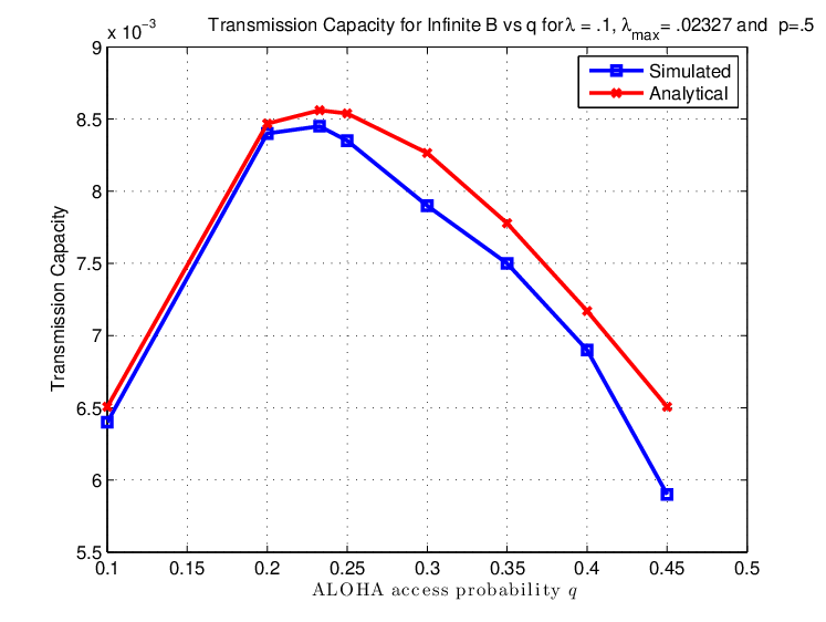
In this section, we present some numerical examples to illustrate our theoretical results. In all simulations we use energy arrival rate $p=.5$, $\alpha=3$, $\theta=2$, and $d=2$, such that $\lambda_{max}=.023$, except for Fig. 5, where $\alpha=3$, $\theta=1$, and $d=1$, and $\lambda_{max}=.2632$ is used. In Figs. 4 and 5, we plot the transmission capacity for ALOHA MAP for $B=\infty$ with $\frac{\lambda_{max}}{\lambda}>p$ and $\frac{\lambda_{max}}{\lambda}\leq p=0.5$, respectively, from which we can see that for $\frac{\lambda_{max}}{\lambda}\leq p$, the optimal transmission probability is $q^{\star}=\frac{\lambda_{max}}{\lambda}$, while in the other case $p\leq q^{\star}\leq 1$, as derived in Theorem 1. In Figs. 6 and 7, we plot the transmission capacity for ALOHA MAP with $B=1$, and $B=5$, respectively. From Figs. 4, 6, and 7, we can see that as $B$ increases $q^{\star}$ goes from $0.3$ for $B=1$ to $0.23$ for $B=\infty$ for fixed set of parameters. Finally, in Fig. 8, we plot the back-off probability with CSMA MAP as a function of $\lambda$. Following Theorem 5, we see that for $\lambda=.01$ and $.035$ for which $\frac{-\ln(p)\lambda_{max}}{\lambda}>p$, back off probability is equal to $1-\exp^{-\left(\frac{p\lambda}{\lambda_{max}}\right)}$, while for $\lambda=.05$ and $.1$, where $\frac{-\ln(p)\lambda_{max}}{\lambda}\leq p$, it satisfies the equation $P_{b}=1-\exp^{-\left(\frac{r(1-P_{b})\lambda}{\lambda_{max}}\right)}$.

In this paper we considered ALOHA and CSMA MAP for an ad hoc network, and derived optimal transmission probability for ALOHA MAP, and back-off and outage probability expressions for CSMA MAP, when each node in the network harvest energy from nature. We characterized the dependence of system throughput on the energy arrival rate, and derived system parameters for optimal performance. In this work, we assumed that each transmitter attempts to transmit with same probability irrespective of the current energy state. With finite battery capacity, it makes more sense to transmit aggressively in high energy states and vice-versa. Analyzing energy aware transmission strategies remains an important problem to solve in future with energy harvesting nodes.

References

- [1] S. Weber, X. Yang, J. Andrews, and G. de Veciana, “Transmission capacity of wireless ad hoc networks with outage constraints,” IEEE Trans. Inf. Theory, vol. 51, no. 12, pp. 4091–4102, Dec. 2005.
- [2] F. Baccelli, B. Blaszczyszyn, and P. Muhlethaler, “An aloha protocol for multihop mobile wireless networks,” IEEE Trans. Inf. Theory, vol. 52, no. 2, pp. 421–436, Feb. 2006.
- [3] O. Ozel, K. Tutuncuoglu, J. Yang, S. Ulukus, and A. Yener, “Transmission with energy harvesting nodes in fading wireless channels: Optimal policies,” CoRR, vol. abs/1106.1595, 2011. [Online]. Available: http://arxiv.org/abs/1106.1595
- [4] K. Tutuncuoglu and A. Yener, “Sum-rate optimal power policies for energy harvesting transmitters in an interference channel,” CoRR, vol. abs/1110.6161, 2011. [Online]. Available: http://arxiv.org/abs/1110.6161
- [5] H. Erkal, F. M. Ozcelik, and E. Uysal-Biyikoglu, “Optimal offline broadcast scheduling with an energy harvesting transmitter,” CoRR, vol. abs/1111.6502, 2011. [Online]. Available: http://arxiv.org/abs/1111.6502
- [6] A. Sinha and P. Chaporkar, “Optimal power allocation for renewable energy source,” CoRR, vol. abs/1110.2288, 2011. [Online]. Available: http://arxiv.org/abs/1110.2288
- [7] R. Vaze, “Competitive ratio analysis of online algorithms in energy harvesting communication system,” CoRR, Dec. 2011. [Online]. Available: http://arxiv.org/abs/1112.5557
- [8] F. Iannello, O. Simeone, and U. Spagnolini, “Medium access control protocols for wireless sensor networks with energy harvesting,” CoRR, vol. abs/1112.2409, 2011.
- [9] V. Sharma, U. Mukherji, V. Joseph, and S. Gupta, “Optimal energy management policies for energy harvesting sensor nodes,” IEEE Trans. Wireless Commun., vol. 9, no. 4, pp. 1326 –1336, Apr. 2010.
- [10] J. Jeon and A. Ephremides, “The stability region of random multiple access under stochastic energy harvesting,” in ISIT, 2011, pp. 1796–1800.
- [11] K. Huang, “Throughput of wireless networks powered by energy harvesting,” CoRR, vol. abs/1111.5799, 2011.
- [12] M. K. Hanawal, E. Altman, and F. Baccelli, “Stochastic geometry based medium access games in mobile ad hoc networking,” in IEEE International Conference on Computer Communication, Infocom 2012, 25-29 Mar. 2012.
- [13] D. Stoyan, W. Kendall, and J. Mecke, Stochastic Gemoetry and its Applications. John Wiley and Sons, 1995.
- [14] F. Baccelli, B. Blaszczyszyn, and P. Muhlethaler, “An Aloha protocol for multihop mobile wireless networks,” IEEE Trans. Inform. Theory, vol. 52, no. 2, pp. 421–436, 2006.
- [15] A. MacKenzie and S. Wicker, “Stability of multipacket slotted aloha with selfish users and perfect information,” in INFOCOM 2003, vol. 3, Mar.-Apr. 2003, pp. 1583 – 1590.
- [16] M. Kaynia and N. Jindal, “Performance of aloha and csma in spatially distributed wireless networks,” in IEEE International Conference on Communications, 2008. ICC ’08., may 2008, pp. 1108 –1112.
- [17] M. Kaynia, N. Jindal, and G. Oien, “Improving the performance of wireless ad hoc networks through mac layer design,” IEEE Trans. Wireless Commun., vol. 10, no. 1, pp. 240 –252, Jan. 2011.
- [18] R. Vaze, “Throughput-delay-reliability tradeoff with ARQ in wireless ad hoc networks,” IEEE Trans. Wireless Commun., vol. 10, no. 7, pp. 2142 –2149, Jul. 2011.
- [19] R. Ganti and M. Haenggi, “Spatial and temporal correlation of the interference in aloha ad hoc networks,” IEEE Commun. Lett., vol. 13, no. 9, pp. 631 –633, sept. 2009.
- [20] G. Grimmett, Percolation. Springer-Verlag, 1980.