Filter-and-Forward Transparent Relay Design for OFDM SystemsThanks: †Corresponding authorThanks: The authors are with the Dept. of Electrical Engineering, KAIST, Daejeon 305-701, South Korea. E-mail:{dg.kim@, jyseo@, and ysung@ee.}kaist.ac.kr. This research was also supported by the KCC (Korea Communications Commission), Korea, under the R&D program supervised by the KCA (Korea Communications Agency) (KCA-2012-11-911-04-001). Some part of the paper was presented in [1].
Abstract
In this paper, the filter-and-forward (FF) relay design for orthogonal frequency-division multiplexing (OFDM) transmission systems is considered to improve the system performance over simple amplify-and-forward (AF) relaying. Unlike conventional OFDM relays performing OFDM demodulation and remodulation, to reduce processing complexity, the proposed FF relay directly filters the incoming signal in time domain with a finite impulse response (FIR) and forwards the filtered signal to the destination. Three design criteria are considered to optimize the relay filter. The first criterion is the minimization of the relay transmit power subject to per-subcarrier signal-to-noise ratio (SNR) constraints, the second is the maximization of the worst subcarrier channel SNR subject to source and relay transmit power constraints, and the third is the maximization of data rate subject to source and relay transmit power constraints. It is shown that the first problem reduces to a semi-definite programming (SDP) problem by semi-definite relaxation and the solution to the relaxed SDP problem has rank one under a mild condition. For the latter two problems, the problem of joint source power allocation and relay filter design is considered and an efficient algorithm is proposed for each problem based on alternating optimization and the projected gradient method (PGM). Numerical results show that the proposed FF relay significantly outperforms simple AF relays with insignificant increase in complexity. Thus, the proposed FF relay provides a practical alternative to the AF relaying scheme for OFDM transmission.
Index Terms:
Linear relay, filter-and-forward, amplify-and-forward, OFDM systems, semi-definite programmingI Introduction
Recently, relay networks have drawn extensive interest from the research community because they play an important role in enlarging the network coverage and improving the system performance in current and future wireless networks. Indeed, LTE-Advanced adopts relays for coverage extension and performance improvement [2]. There are several well-known relaying schemes such as AF, decode-and-forward (DF), and compress-and-forward (CF) [3, 4, 5]. Among the relaying schemes, the AF scheme (i.e., simple repeater) is the simplest and is suitable for cheap relay deployment under transparent†† † Transparent operation means that the destination node does not know the existence of the relay node, and this operation is suitable for cheap AF relays [2]. operation [2]. Recently, there have been some efforts to extend this simple AF scheme to a linear filtering relaying scheme, i.e., an FF scheme, to obtain better performance than the AF scheme while keeping the benefit of low computational complexity of the AF scheme [6, 7, 8, 9, 10, 11]. It has been shown that the FF scheme can outperform the AF scheme considerably. However, most of the previous works on the FF relay have been done for single-carrier transmission, whereas most of the current wireless standards adopt OFDM transmission. Thus, in this paper, we propose direct FF relaying for OFDM transmission instead of using conventional OFDM relays which OFDM-demodulate the incoming signal, amplify or decode the demodulated signal, OFDM-remodulate the processed signal and transmit the remodulated OFDM signal to the destination [12, 13, 14, 15]. In the proposed scheme, the incoming signal to the relay is FIR filtered at the chip rate of the OFDM modulations in time domain and the filtered signal is directly forwarded to the destination. In this way, the necessity of OFDM processing at the relay is eliminated, but the overall performance can still be improved over the AF scheme by a properly designed relay filter.

I-A Our Approach and Contributions
In the paper, we consider three meaningful criteria for the FF relay design for OFDM systems, minimization of power consumption at the relay, maximization of the worst subcarrier SNR, and maximization of the data rate, under the scenario of single-input single-output (SISO) communication as the first step in this research direction. (The multiple-input multiple-output (MIMO) communication case is beyond the scope of this paper and will be studied as a future work.) Our contributions on this topic are summarized in the below.
- •
First, exploiting the eigen-property of circulant matrices and the structure of Toeplitz filtering matrices, we derived necessary expressions for the problem formulation such as the subcarrier SNR and the relay transmit power in terms of the design variables of the relay filter coefficients and source power allocation, and formulated the above problems explicitly based on the derived expressions.
- •
In the case of the first problem of relay power minimization under per-subcarrier SNR constraints, we showed that the problem is expressed as a semi-definite relaxation problem. That is, the original non-convex FF relay design problem is approximated by a convex SDP problem. Furthermore, in this case we showed that the solution to the relaxed SDP problem is the same as that to the original problem under a mild condition.
- •
For the second design criterion, we formulated the problem of joint design of the relay filter and the source power allocation for the worst subcarrier SNR maximization subject to source and relay power constraints and provided an efficient iterative algorithm to solve this problem based on alternating optimization. The provided algorithm consists of two steps at each iteration, optimizing the relay filter to maximize the worst subcarrier SNR for given power allocation and optimizing the source power allocation to maximize the worst subcarrier SNR for a given relay filter, and guarantees convergence to a locally optimal point, although the convergence to a globally optimal point is not guaranteed. We showed that the first step of the iteration reduces to a SDP problem and the second step of the iteration reduces to a linear programming (LP). The second criterion is closely related to bit error rate (BER) minimization in case of weak or no channel coding in addition to overall quality-of-service (QoS) improvement for subcarrier channels. This is because in the single-user case, bits for one user are distributed across subcarriers and the overall system BER is dominated by the BER of the worst subcarrier channel [16].
- •
For the third problem of joint optimization of the relay filter and the source power allocation for rate maximization, we proposed an efficient algorithm by applying the projected gradient method [17, 18, 19, 11] directly to this constrained optimization problem. The proposed method guarantees the satisfaction of the constraints and convergence to a locally optimal point.
Numerical results show that the proposed FF relay significantly outperforms simple AF relays and furthermore achieves most of the performance gain with not so many filter taps. Thus, the proposed FF relay provides a practical alternative with low complexity to the AF relaying scheme for OFDM transmission.
I-B Notation and Organization
In this paper, we will make use of standard notational conventions. Vectors and matrices are written in boldface with matrices in capitals. All vectors are column vectors. For a matrix , , , , and indicate the complex conjugate, transpose, conjugate transpose, and trace of , respectively. and mean that is positive semi-definite and that is strictly positive definite, respectively. For two matrices and , means that . stands for the identity matrix of size (the subscript is omitted when unnecessary), and denotes a matrix with all zero elements. The notation indicates a Toeplitz matrix with rows and as its first row vector, where is a row vector of size , and means a diagonal matrix with diagonal elements . The notation means that is complex circularly-symmetric Gaussian distributed with mean vector and covariance matrix . denotes the expectation. .
The remainder of this paper is organized as follows. The system model is described in Section II. In Section III, the FF relay design problems are formulated and solved. In Section IV, the performance of the proposed design methods is investigated. Several issues regarding practical implementation of the proposed FF relay are discussed in Section V, followed by the conclusion in Section VI.
II System Model
We consider a full-duplex‡‡ ‡ Please see Section V. relay network composed of a source node (basestation), a relay node and a destination node (terminal station), as shown in Figures 1 and 2, where the source employs OFDM modulation with subcarriers and each link performs SISO communication. We consider the case that the direct link between the source and the destination is seriously faded. Thus, for simplicity, we assume that there is no direct link between the source and the destination and that both the source-to-relay (SR) link and the relay-to-destination (RD) link are frequency-selective channels modeled as multi-tap filters with finite impulse responses. We assume that the relay is an FF relay, i.e., the relay performs FIR filtering on the incoming signal at the chip rate of the OFDM modulation and transmits the filtered output immediately to the destination.§§ § Such an FF scheme requires up and down converters and simple baseband circuitry only. Thus, the FF relay can be regarded as an additional frequency-selective (time-dispersive) channel between the source and the destination. We assume that the order of the FIR filter at the relay does not make the length of the overall FIR channel between the source and the destination larger than that of the OFDM cyclic prefix. Since our focus of using the FF relay in this paper is the transparent relay operation, we assume that the SR channel state is known to the relay and that the RD channel state is unknown to the relay but the RD channel distribution is known to the relay. Such an assumption is reasonable for the transparent relay operation since the relay node does not have its own identity and the destination node does not know the existence of the relay; thus, the destination node does not feedback information to the relay node directly. (Please see Section V regarding how to obtain channel information.)
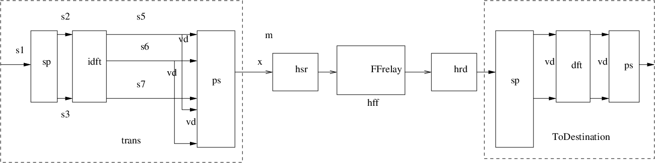
Specifically, at the source, the length data vector of OFDM symbols is given by , where each data symbol is assumed to be a zero-mean independent complex Gaussian random variable with variance , i.e., for . The time-domain signal vector after normalized inverse discrete Fourier transform (IDFT) at the source is given by
| (1) |
where . Let denote the -th row of the normalized IDFT matrix for . Then, can be written as and the covariance matrix of is given by
| (2) |
where is the vector composed of source power assigned to each subcarrier, since
| (3) |
The vector is attached by a cyclic prefix with length , i.e.,
| (4) |
and the cyclic prefix attached sequence is transmitted from the source to the relay through the SR channel. Then, the received baseband signal at the relay is given by
| (5) |
where is the channel tap coefficient vector of the SR channel known to the relay, is the length of the SR FIR channel, and is the additive white Gaussian noise at the relay with . At the relay, the received signal is FIR filtered at the chip rate of the OFDM transmission and then transmitted immediately to the destination. Thus, the output signal at the relay at (chip) time is given by
| (6) |
where is the FIR filter coefficient vector at the relay and is the order of the FIR filter. Note that, when , the FF relay simply reduces to the AF relay. However, when , the FF relay is an extension of the AF relay with some amount of digital processing. Finally, the signal transmitted by the relay goes through the RD FIR channel to the destination. Thus, the received signal at the destination is given by
| (7) |
where is the FIR channel tap coefficient vector for the RD channel, is the order of the RD FIR channel, and is zero-mean white Gaussian noise with variance at the destination. Here, we assume that the channel tap coefficient , , is independent and identically distributed (i.i.d.) according to , i.e., each tap is independently Rayleigh faded, and that the realization is not known to the relay but its distribution is known to the relay. By stacking the output symbols at the relay and the received symbols at the destination, we have the following vectors for the transmitted signal at the relay and the cyclic prefix portion removed received signal vector at the destination, respectively:
| (8) |
where
| (9) | |||||
Under the assumption that , the DFT of the cyclic prefix portion removed received vector of size at the destination is given by
| (10) | |||||
| (11) | |||||
| (12) |
where is the normalized DFT matrix of size , is a circulant matrix generated from the overall Toeplitz filtering matrix from the source to the destination, and is the eigen-decomposition of .
II-A Manipulation for quadratic forms
The received signal form (12) is standard in OFDM transmission, but the form cannot be used directly for relay filter optimization in the next section. Thus, in this subsection, we derive an explicit expression for the received signal , , which facilitates optimization formulation in the next section, based on the following property of circulant matrices [20].
Lemma 1
[20] Let be an circulant matrix with the first row . Then, the eigenvalues of are given by
with the corresponding right eigenvectors
By Lemma 1, to derive the diagonal elements of in (12), we need to know only the first row of in (11). Let the first row of be . Then, is a row vector given by
| (13) |
and the first row of is given by . Since is generated by truncating out the elements of outside the first positions and by moving the lower elements of the truncated part to the lower left of the untruncated matrix, the first row of is simply the first elements of the first row of , i.e., , where is a truncation matrix for truncating out the elements of except the first elements, given by
| (14) |
Now, the diagonal elements of can be obtained by Lemma 1 and are given by
| (15) |
where is the DFT matrix of size . Finally, the received signal in the -th subcarrier at the destination is expressed as
| (16) |
where is the ()-th row of . Thus, the signal and noise parts of are given by
| (17) |
respectively, for .
III Filter-and-Forward Relay Design Criteria and Optimization
In this section, we consider three meaningful FF relay design problems for the relay network employing OFDM transmission described in Section II. First, we consider the FF relay filter design to minimize the transmit power of the FF relay subject to an SNR constraint for each OFDM subcarrier channel when the source power allocation is given. Here, we shall show that the problem can be formulated as a semi-definite relaxation (SDR) problem. That is, the original non-convex FF relay design problem is approximated by a convex SDP problem. Furthermore, in this case we shall show that the solution to the relaxed SDP problem is the same as that to the original problem under a mild condition. With the formulae for the relay transmit power and the subcarrier channel SNR in terms of the relay filter coefficients and source power allocation obtained to solve the first problem, we next consider two more relay design problems. One is the problem of maximizing the worst subcarrier SNR subject to source and relay power constraints and the other is the problem of rate maximization subject to source and relay power constraints. The first criterion aims not only at overall quality-of-service (QoS) improvement for subcarrier channels but also at bit error rate (BER) minimization in case of weak or no channel coding. In the single-user case, bits for one user are distributed across subcarriers and the overall system BER is dominated by the BER of the worst subcarrier channel since the worst error rate dominates the system error rate [16]. Thus, maximization of the worst subcarrier SNR is almost equivalent to minimization of the system BER in the single-user case. For the latter two problems, we consider joint optimization of the relay filter and source power allocation. These two problems are non-convex optimization problems with respect to the relay filter tap coefficients and the source power allocation. Thus, it is not easy to find a globally optimal solution. To circumvent this difficulty, we apply alternating optimzation and the projected gradient method to the worst subcarrier SNR maximization problem and the rate maximization problem, respectively, and propose an efficient iterative algorithm for each problem that converges to a locally optimal point at least.
III-A FF relay transmit power minimization under per-subcarrier SNR constraints
We first consider the problem of designing the FF relay tap coefficient vector to minimize the relay transmit power subject to an SNR constraint per OFDM subcarrier. This problem is formulated as follows:
Problem 1: For given source power allocation , SR channel , RD channel static information , FF relay filter order , and a set of desired minimum SNR values for subcarrier channels ,
| (18) |
where is the relay transmit power and is the SNR of the -th subcarrier channel.
To solve Problem 1, we need to express each term in the problem as a function of the design variable . First, let us derive the SNR on the -th subcarrier channel in the received signal (16) at the destination. Note that the signal and noise parts in (17) are represented in terms of the relay filtering matrix . The representation of SNR in terms of is redundant since the true variable is embedded in . Thus, we need reparameterization of SNR in terms of , and this can be done based on (17) by exploiting the Toeplitz structure of as follows. Using (17), we first express the received signal power at the destination in terms of as
| (19) | |||||
where
is a matrix composed of the first rows of ; and
| (20) |
Here, (a) holds due to the assumption of independence of the signal and the RD channel coefficients; (b) holds due to the assumption¶¶ ¶ The i.i.d. assumption for is not necessary. More general cases such as correlated and deterministic can be included in the proposed framework with slight change in the derivation. of (see (13)) ; (c) and (d) hold due to ; (e) holds due to ; and (f) is obtained because and thus . The key point of the derivation of (19) is that the received signal power at the -th subcarrier channel is represented as a quadratic form of the design variable . Next, consider the received noise power for the -th subcarrier channel. Using similar techniques to those used to obtain (19), we can express the received noise power based on the noise part in (17) as
| (21) | |||||
where and is given by
| (22) |
Here, be the -th row of and the size of each in (22) is . (It is easy to verify that due to the Toeplitz structure of .) Based on (19) and (21), the SNR of the -th subcarrier channel is expressed as
| (23) |
Next, consider the relay transmit power. Using (8), we obtain the relay transmit power in a similar way as
| (24) | |||||
where , and is obtained similarly to (2) based on (3). The last equality holds since the power is a real-valued quantity.
Now, based on (19), (21) and (24), Problem 1 can be restated as follows:
| (25) |
The above problem is not a convex problem. However, the problem can still be solved efficiently by using convex optimization techniques. Let . Then, by using and relaxing the rank one constraint for , the problem (25) can be reformulated as follows:
Problem 1′:
| (26) | |||||
| s.t. | |||||
where , , and .
Note that by relaxing the rank one constraint for , Problem 1 is converted to Problem 1′, which is a semi-definite program (SDP) [21] and it can be solved efficiently by using the standard interior point method for convex optimization [21], [22]. With an additional constraint , Problem 1′ is equivalent to the original Problem 1. That is, if the optimal solution to Problem 1′ has rank one, then it is also the optimal solution to Problem 1. However, there is no guarantee that an algorithm for solving Problem 1′ yields the desired rank one solution. In such a case, randomization techniques [23] can be used to obtain a rank-one solution from . However, for this specific problem related to the transparent FF relay design, we provide a stronger result, stated in the following theorem.
Theorem 1
If all the desired SNR constraints except one are satisfied with strict inequality, then the nontrivial optimal solution of Problem 1′, which is a relaxed version of Problem 1, always has rank one.
Proof : See the appendix.
Note that the condition in Theorem 1 is mild and is satisfied in many cases. Thus, solving Problem 1′ directly yields the solution to the original power minimization problem under subcarrier SNR constraints in many cases.
III-B Worst subcarrier SNR maximization
Now, we consider the second FF relay design problem of maximizing the SNR of the worst subcarrier channel under transmit power constraints. As mentioned already, this problem is closely related to BER minimization in case of weak or no channel coding in addition to minimum QoS improvement. To be complete, for this important problem we consider not only relay filter optimization but also optimal source power allocation. The joint optimization yields a further gain over the relay filter optimization only, as seen in other joint optimization [13, 24, 25]. The problem of joint source power allocation and FF relay filter design to maximize the worst subcarrier SNR subject to total source and relay transmit power constraints is formulated as follows:
Problem 2: For given SR channel , RD channel statistic information , FF relay filter order , maximum available source transmit power , and maximum available relay transmit power , optimize the relay filter and the source power allocation in order to maximize the worst subcarrier SNR:
| (27) |
Note that Problem 2 is a complicated non-convex optimization problem. There exist several methods that can find the optimal solution of a non-convex optimization problem as long as the cost function is not too complicated [26, 27]. However, such methods require high computational complexity. Hence, we here approach the problem by using a suboptimal alternating optimization technique for computational efficiency. That is, first the source power allocation is initialized properly and Problem 2 is solved to optimize the relay filter for given source power allocation. (This problem is defined as Problem 2-1.) Then, with the given relay filter tap coefficients obtained by solving Problem 2-1, the source power allocation is optimized. (This problem is defined as Problem 2-2.) The two problems are solved in an alternating fashion until the iteration converges. Let us consider Problem 2-1 first. Problem 2-1 can be written explicitly based on (23) and (24) as follows:
Problem 2-1: For given source power allocation , SR channel , RD channel static information , FF relay filter order , and maximum available relay transmit power ,
| (28) |
By introducing a slack variable , the above max-min problem can be rewritten as
| (29) | |||||
| s.t. | |||||
Note that this is a non-convex problem. Again, as in the previous subsection, we convert the problem to a tractable convex problem by semi-definite relaxation as follows:
| (30) | |||||
| s.t. | |||||
where , , and are already defined in Problem 1′. In the problem (30), the rank constraint is dropped by semi-definite relaxation as in Problem 1′. Note that the relaxed optimization problem is quasi-convex, i.e., for given the problem is convex. The solution of the quasi-convex optimization problem can be obtained by solving its corresponding feasibility problem [28]:
| Find | (31) | ||||
| s.t. | |||||
The feasible set in the problem (30) is convex for any value of . Let be the optimal value of the problem (30). Then, we can find the solution to the problem (30) by using the fact that the feasibility problem (31) is feasible for , whereas it is not feasible for . Based on this, we propose a simple bisection algorithm to solve the problem (30), a relaxed version of Problem 2-1, as follows:
Algorithm 1
Choose some appropriate interval s.t. .
Step 1: Set .
Step 2: Solve the feasibility problem (31) for . If it is feasible, . Otherwise, .
Step 3: Repeat Steps 1 to 2 until .
Here, is the allowed error tolerance for . Note that the above feasibility problem is a standard SDP problem, which can be solved easily by the interior point method [22]. Due to the relaxation, the matrix obtained by solving the relaxed optimization problem may not have rank one in general. In such a case, randomization techniques can be applied to find a rank-one solution.
When we optimize only the relay filter to maximize the worst subcarrier SNR for given source power allocation, we can simply use Algorithm 1 only. However, for joint optimization of the relay filter and source power allocation by alternating optimization, we need to consider Problem 2-2, which is given as follows:
Problem 2-2: For given FF relay filter , SR channel , RD channel statistic information , maximum allowed source transmit power , and maximum allowed relay transmit power ,
| (32) |
where is the allowed minimum for the worst subcarrier SNR.
The constraint in (32) is introduced intentionally to guarantee that the proposed alternating algorithm yields a monotone non-decreasing sequence of the worst subcarrier SNR values. (This will become clear shortly.) By introducing a slack variable and using (23) and (24), Problem 2-2 can be rewritten as follows:
| (33) | |||||
| s.t. | |||||
| (34) | |||||
Note that without the relay power constraint (34), the above problem is a simple linear programming (LP) with respect to and . Indeed, the problem is an LP since the relay power constraint can also be written as a linear form in terms of , as shown below. The relay power (24) can be rewritten as
| (35) | |||||
where is defined in (22), and is the cyclic prefix extended IDFT matrix given by
Here, (a) can be verified by using (9) and (b) is due to the assumption of for . Using the new expression (35) for the relay transmit power, we obtain an LP optimization problem for the source power allocation from the problem (33) as
| (36) | |||||
| s.t. | |||||
| (37) | |||||
where , , and . Since the problem (36) is a LP problem, Problem 2-2 can easily be solved by a standard convex optimization solver.
Now, combining Problems 2-1 and 2-2, we present our alternating optimization algorithm for the joint source power allocation and relay filter design problem to maximize the worst subcarrier SNR, given in Algorithm 2.
Algorithm 2
Given parameters: , , , , and .
Step 1: Initialize for . For example, .
Step 2: Solve Problem 2-1 with Algorithm 1.
Step 3: Set the allowed minimum for the worst subcarrier SNR in Problem 2-2 as the maximum value obtained from Algorithm 1 in Step 2.
Step 4: For given and from Steps 2 and 3, solve Problem 2-2 by solving the problem (36) to obtain new , .
Step 5: Go to Step 2. Here, set of Problem 2-1 as the solution to Problem (36) in Step 4.
Step 6: Repeat Steps 2 to 5 until .
Here, is the allowed error tolerance for . Note that at each iteration the value of the worst subcarrier SNR is monotone non-decreasing. This is because the maximum value of the previous step is set as a lower bound of the current step and the problem at the current step is feasible since the previous combination of and achieves the current lower bound. Since is monotone non-decreasing and upper bounded because of finite transmit power and , the proposed algorithm converges to a locally optimal point by the monotone convergence theorem. Although convergence to the global optimum is not guaranteed, it will be seen in Section IV that the proposed joint design approach improves the performance significantly over the relay filter optimization only.
III-C Rate maximization
The third design criterion that we consider in this paper is rate maximization. This problem is especially interesting when high data rates are the main goal of the system design. Again for this rate maximization problem, we consider joint optimization of the relay filter and source power allocation. Based on the expressions for the subcarrier SNR and the relay power obtained in the previous subsections, the problem is formulated as follows:
Problem 3: For given , , , , and ,
| (38) | |||||
| s.t. | (39) | ||||
| (40) |
When the relay filter is given, an optimal solution to the problem is simply given by the well-known water-filling strategy for parallel Gaussian channels [29]. However, the freedom to design the relay filter and the dependence of the relay transmit power on the source power allocation make the problem far more difficult than a simple water-filling problem. Note that with as the design variable, the problem is a non-convex problem. Due to the structure of the cost function, it is not easy to convert the problem to a certain convex problem as in the previous subsections. Thus, as in [11], we adopt a direct numerical method to solve this problem based on the projected gradient method (PGM) which consists of a gradient descent step for cost reduction and a projection onto the constraint set at each iteration and is widely used for constrained optimization [17, 18, 19, 11]. To apply the PGM, we rewrite Problem 3 as follows:
| (41) | |||||
| s.t. | (42) | ||||
| (43) |
where , , , and . Then, the joint design variable vector and the cost function for the PGM are respectively given by
| (44) | |||||
| (45) |
The gradient of w.r.t. can be obtained as
| (46) |
where , , and . The constraint set defined by (42) is a half-space for defined by a hyperplane with no restriction on and thus is a convex set of . However, the constraint set defined by (43) is not convex but biconvex w.r.t. and . That is, is an ellipsoid for for given as seen in (43) and is a half-space for for given as seen in (37). Thus, projection onto can be implemented effectively by successive projections: one projecting onto and the other projecting onto the ellipsoid of for the given projected by the first projection. Based on these projections and (46), we can apply the PGM to Problem 3 in a similar way to that in [11]. It is guaranteed that the PGM yields a unique globally optimal solution when it is applied to a convex optimization problem [19]. However, Problem 3 is not a convex problem, and thus the proposed algorithm does not guarantee convergence to a globally optimal point. However, numerical results show that the algorithm converges and works well.
IV Numerical results
In this section, we provide some numerical results to evaluate the performance of the FF relay design methods proposed in Section III. We considered a relay network with an OFDM transmitter, an FF relay, and a destination node, as described in Section II. Throughout the simulation, we fixed the number of OFDM subcarriers as with a minimal cyclic prefix covering the overall FIR channel length in each simulation case. In all cases, both SR and RD channel tap coefficients ’s and ’s were generated i.i.d. according to the Rayleigh distribution, i.e., for and for ; the relay and the destination had the same noise power ; and the source transmit power was 20 dB higher than the noise power, i.e., . (From here on, all dB power values are relative to .)
We first examined the performance of the first FF relay design method, provided in Problem 1′, to minimize the relay transmit power subject to required SNR constraints on subcarrier channels. Fig. 3 shows the corresponding result.

 (a)
(b)
(a)
(b)
Here, the SR channel length and the RD channel length were set as .
We chose from 32 subcarriers. It is known that for a set of randomly realized propagation channels, it is not easy to always guarantee the desired SNR for every subcarrier channel when the desired SNR value is high [8]. Thus, in Figures 3 (a) and (b), each line was plotted when Problem 1′ was feasible for more than 50 % out of 1000 random channel realizations for the given minimum required SNR value for all the subcarrier channels in , and the plotted value is the relay transmit power averaged over the feasible channel realizations. It is seen that the required relay transmit power for the same minimum SNR required by the FF relay is significantly reduced when compared to that required by the AF relay. Fig. 3 (b) shows the relay transmit power versus the relay filter length for various desired minimum SNR values. It is seen that the required relay transmit power for the same desired minimum SNR decreases monotonically with respect to , as expected, and the FF relay achieves most of the gain with only a few FF filter taps.

 (a)
(b)
(a)
(b)
Next, we evaluated the performance of the second FF relay design method to maximize the worst subcarrier SNR subject to transmit power constraints. First, we considered the relay filter optimization only for given equal source power allocation, i.e., , based on Algorithm 1. Fig. 4 shows the result. For the figure, 500 channels were randomly realized with and each plotted value is the average over the 500 channel realizations. Here, an OFDM-processing per-subcarrier AF relay is used as an upper bound of the FF relay. ∥∥ ∥ The derivation of the OFDM-processing per-subcarrier AF relay design for the worst subcarrier SNR maximization is available at http://wisrl.kaist.ac.kr/papers/wisrltechrep2013feb01.pdf. As in the previous case of relay transmit power minimization, the gain by the FF relay over the AF relay () is significant. Note in Fig. 4 (a) that the performance of the FF relay improves as the FF relay filter length increases, and eventually converges to the performance of the OFDM-processing per-subcarrier AF relay designed for the same objective in the range of low and intermediate relay power. This is because what the FF relay does is spectral shaping of the overall channel essentially (see Fig. 5 (a)) and this spectral shaping can be done maximally with the OFDM-processing per-subcarrier AF relay. Note that most of the gain is achieved by only a few filter taps for the FF relay and the performance of the FF relay approaches the upper bound quickly in the range of low and intermediate relay power. On the other hand, it is seen in Fig. 4 (a) that the performance of the FF relay saturates in the high relay transmit power range for . At high SNR, precise filtering is required to put the relay power exactly on channel notches to maximize the worst-subcarrier SNR and the situation is much more strict than the low SNR case in which the channel notches are immersed in the noise floor. The observed increased gap between the OFDM-processing relay and the FF relay in the high relay power range implies that the proposed algorithm can be stuck at some local optimum not at the exact filtering point easily in the the high relay power range. However, the FF scheme still provides far better perfomance than the AF scheme even in this case, and furthermore the practical operating SNR may not be so high to experience such a saturation problem.**** ** Recall that with BPSK or QPSK the required SNR values for uncoded BER 10-3 and 10-6 are 6.8 dB and 10.5 dB, respectively. Thus, the saturation around 10 dB minimum SNR may not cause a problem in practical situations.

 (a)
(b)
(a)
(b)

 (a)
(b)
(a)
(b)
Fig. 5 (a) shows several frequency responses of interest for a set of randomly realized channel vectors and with . ( and .) The frequency response of is the frequency response of the original channel from the source to the destination and the frequence response of is the shaped channel response by the relay filter desinged by Algorithm 1. Note that the notches of the original channel response are filled by the frequency shaping by the relay filter in order to maximize the worst subcarrier SNR and this shaping elaborates as the filter order increases. Fig. 5 (b) shows the impact of the channel order . From Fig. 5 (b), it is deduced that the overall channel order of 5 with already presents quite complicated frequency selectivity and therefore the complexity of frequency selectivity caused by higher channel orders does not impact much on the worst subcarrier SNR maximization when the minimum required SNR is not too high.
We next evaluated the performance of the joint source power allocation and FF relay filter design method to maximize the worst subcarrier SNR, provided in Algorithm 2, and the result is shown in Fig. 6. Again, the OFDM-processing per-subcarrier AF relay was used as a performance upper bound. It is seen that the joint optimization method significantly outperforms the optimization of the relay filter only presented in Algorithm 1. As mentioned in the previous section, the worst subcarrier SNR maximization is closely related to BER minimization. We investigate the BER performance corresponding to Fig. 6 (a) and the result is shown in Fig. 6 (b). Here, we assumed uncoded QPSK modulation for each subcarrier channel. From the result of Fig. 6 (a), we knew the SNR of each subcarrier channel of the total subcarrier channels for the designed FF relay filter and source power allocation. Based on this, we computed the subcarrier BER based on the SNR of each subcarrier and averaged all the subcarrier channel BERs to obtain the overall BER. Although there is a noticeable degradation from the OFDM-processing per-subcarrier AF relay at the high SNR, the FF relay significantly improves the BER performance over the AF relay.

Next, we evaluated the performance of the third FF relay design method, provided in Section III.C, to maximize the sum rate of subcarrier channels subject to source and relay transmit power constraints. The result is shown in Fig. 7. As a performance upper bound, we considered the method in [12] which does full OFDM processing and subcarrier reordering for rate maximization with full knowledge of the SR and RD channel state. It is observed that the proposed FF relay yields a considerable gain over the AF relay. However, the FF relay shows a performance loss when compared to the OFDM-processing method. This loss results from the incapability of the FF relay of subcarrier reordering and the lack of the knowledge of the RD channel state.
Finally, we examined the robustness of the proposed FF relay design methods, Algorithm 2 and the proposed rate maximization algorithm, against channel information mismatch. We considered two types of channel information error again with . One is the RD channel statistic mismatch and the other is the SR channel state mismatch. For the RD channel statitic mismatch, still the i.i.d. RD channel model with and for all taps was used to run Algorithm 2 and the proposed rate maximization algorithm, but the true RD channel was generated randomly according to a different channel statistic, i.e., different and/or different channel power profile. For the SR channel state mismatch, we modeled the available information for the SR channel as , where is the channel information error vector. Here, the true channel coefficient was generated i.i.d. according to for , as mentioned already, and the channel information error was generated i.i.d. according to for . Thus, is the relative power of the channel information error to the power of the true channel tap. Fig. 8 (a) shows the worst subcarrier SNR obtained by Algorithm 2 (averaged 500 over channel realizations) versus the relay transmit power in the case of RD channel static information mismatch and correct SR channel state information. It is seen that the proposed FF relay design method is robust against the channel static mismatch. Fig. 8 (b) shows the impact of the SR channel mismatch on Algorithm 2 with the correct RD static information. As expected, the AF case is most robust against the SR channel information error since it has only one tap. As the number of the FF filter taps increases, there is noticeable performance degradation in the case of the SR channel static mismatch. Figures 8 (c) and (d) show the impact of the RD channel static mismatch and the SR channel state mismatch on the proposed rate maximization algorithm, respectively. Similar behavior is seen as in the worst subcarrier SNR maximization. In both cases, the algorithms are more robust against the RD static mismatch than against the SR state mismatch. Thus, accurate channel estimation of the SR state is necessary. Fortunately, in most cellular communication systems, there exist pilot signals from the basestation which can be used for channel estimation and the SR channel state can be estimated accurately at the relay by using the pilot signals.

 (a)
(b)
(a)
(b)

 (c)
(d)
(c)
(d)
V Discussion
In this section, we discuss several practical issues to implement the proposed full-duplex FF relay. First, let us consider the full-duplex operation. The main advantage of AF relays (i.e., simple reapters) is that they can be operated in the full-duplex mode, and this full-duplex operation incurs no rate reduction inherent to half duplexing. In the full-duplex operation, however, we have the problem of self-interference; i.e., the transmitted signal from the relay is fed back to the receiver of the relay. However, this self-interference problem already exists with full-duplex AF relays. There exists vast literature on mitigation of self-interference for AF relays [30, 31, 32, 33]. It is shown in [30] that echo cancellation combined with the physical separation of transmission and reception antennas at the relay can effectively solve the self-interference problem of full-duplex relays. In the case that interference cancellation is employed at AF relays already, the additional processing for full-duplex FF over full-duplex AF is insignificant because of the already existing up and down conversion and baseband processing for echo cancellation for full-duplex AF relays.
Next consider the availability of the channel information assumed in the previous sections. In many research works for relays, it is assumed that all channel information is available at the transmitter and the relay. For a non-transparent relay, this assumption is valid since the relay has its own identity and can transmit its own pilot signal to terminal stations and the relay can get feedback from terminal stations. However, for the cheap transparent operation, the relay does not have a physical identity and does not receive any feedback for terminal stations. Although the transparent relay is invisible to terminal stastions, there still exists a control communication link between the basestation and the transparent relay in real world systems for maintenance purposes; Basic relay operation commands from the basestation should be delivered to the relay and operation condition information should be fed back to the basestation from the relay. In addition to this basestation-relay control communication link, there exists a low-rate robust control link from terminal stations to the basetation in all cellular networks.†††† †† The control channel typically operates at a low rate. It compensates low signal power with long bit duration. Thus, although the direct link from the basestation to the terminal station is seriously faded, we can still assume that the control link operates properly. Typically, through this link, channel quality indication (CQI) and/or channel state information (CSI) is fed back to the basestation. Exploiting these two control links and the (typically existing) pilot signal from the basestation, one can estimate the necessary channel information assumed in the previous sections, as follows.
Step 1. From the pilot signal transmitted from the basestation, the relay estimates the SR channel state immediately. For example, one can use preamble signals attached in time domain to OFDM signals. There are several time-domain channel estimation techniques for OFDM signals not requiring ODFM processing.
Step 2. The relay filters the incoming signal with the FIR response and transmits the filtered signal to the destination.
Step 3. The destination does not know the existence of the relay in the transparent mode, but what the destination receives for the pilot portion is under the assumption that the SD channel strength is negligible. As usual, the destination node estimates the channel based on the pilot signal . The estimated channel at the relay is then .
Step 4. As in most cellular systems, the destination node feedbacks the CSI to the basestation via the available uplink control channel.
Step 5. The FF relay also feedbacks the SR CSI and its filter response to the basestation via the available control channel between the basestation and the relay.
Step 6. The basestation now has , and . It can simply deconvolve from to obtain . In this stage, it seems more practical and robust to extract and use the stastic of as in this paepr since the CSI is prone to phase errors in the RF circuitries at the relay and communication delays. For example, the delay spread and the channel gain magnitude information can be extracted as in the previous sections.
Step 7. The basestation computes the FF relay filter response (based on the results in the previous sections) and downloads the information to the relay via the control channel between the basestation and the relay. In this case, the information does not need to be fed back to the base station from the relay since the base station already has . In this way, computational burden is moved to the basestation and this strategy seems reasonable for the joint optimization considered in Sections III-B and III-C.
As seen in the above, a practical implementation of the proposed FF scheme is possible and does not require any standard change.
Finally, we consider the possibility of extension of the FF relay to the broadcasting situation in which the basestation serves several terminal stations in the relay cell simultaneously. In this paper, we assumed channel state information for the SR channel and channel statistic information for the RD channel. The assumption of channel statistic information for the RD channel makes the proposed FF relay design method useful for the broadcasting purpose. Suppose that the basestation acquires the channel information from each terminal station by the method in the above paragraph. Then, the basestation has the RD channel information from all terminal stations in the relay cell. The basestation can select and schedule terminal stations with similar channel statistics and designs the relay filter accordingly. In this way, the proposed FF relay scheme can be applied to the broadcasting scenario since the proposed design methods do not require exact CSI or the phase of the channel gain for the RD channel and are robust against the RD channel static mismatch. In this broadcasting scenario, the worst subcarrier SNR maximization in Section III-B improves QoS fairness among users and the rate maximization in Section III-C increases the overall system sum rate.
VI Conclusion
In this paper, we have considered the FF relay design for OFDM systems for transparent relay operation to compromise the performance and complexity between the simple repeater and the full OFDM-processing relay. We have considered three FF relay design criteria of minimizing the relay transmit power subject to per-subcarrier SNR constraints, maximizing the worst subcarrier SNR subject to transmit power constraints, and maximizing the data rate subject to transmit power constraints. We have proposed an efficient algorithm for each of the three criteria based on convex relaxation, alternating optimization and the projected gradient method. The proposed FF relay significantly outperforms the simple repeater with slight increase in complexity and the same operating condition, and thus provides an effective alternative to the simple repeater. In this paper, we assumed SISO-OFDM systems. However, most current OFDM systems employ MIMO communications and thus, extension to the MIMO case is left as a future work.
Appendix
Proof of Theorem 1
By introducing a slack variable , we convert Problem 1′ to the following equivalent problem:
| (47) | |||||
| s.t. | (48) | ||||
| (49) | |||||
| (50) | |||||
| (51) |
The Lagrange dual function for the above problem is given by
| (52) |
where , , and are the dual variables associated with (48), (49), (50), and (51), respectively. If or , then the dual function value is minus infinity or we have trivial solutions and/or . Thus, for the nontrivial feasibility of and , we have and . Then, the Lagrange dual function is easily obtained as and the corresponding dual problem is given by
| (53) | |||||
| s.t. |
Let and be the optimal values for the problem. ( and are automatically determined based on these quantities. The dependence of on and is not shown explicitly for notational simplicity from here on.) From the complementary slackness conditions for (48) and (49), we have
| (54) |
which is equivalent to
| (55) |
Since the problem (47-51) is a convex optimization problem, the duality gap is zero, i.e., . Thus, both the first and second terms in the left-hand side (LHS) of (55) are nonnegative since and . (The trace of the product of two positive semi-definite matrices is nonnegative [34].) Therefore, and . It is obvious that for a nontrivial from , i.e., the matrix does not have full rank. This is because , where is the eigen-decomposition of . (If , then .) Note from (55) that
| (56) |
where is a positive definite matrix defined in (24), is a positive semi-definite matrix defined in (21), and defined in (19) is a rank-one matrix by Lemma 2. Now, under the assumption that all the SNR constraints except one are satisfied with strict inequality, we have for some and from the complementary slackness conditions. In this case, is given by
| (57) |
Due to the structure of in (57), the rank of is larger than or equal to . Since , . Since (where is the eigen-decomposition of ), we conclude that has nullity and thus has rank one under the assumption of Theorem 1.
Lemma 2
If , has rank one regardless of the value of .
Proof of Lemma 2: Recall that (see (19) and (26))
| (58) |
Let in (20) be partitioned as . Note that and are Toeplitz matrices and that is also a Toeplitz matrix regardless of due to the property of DFT matrices. It is not difficult to show that is a Toeplitz matrix, where denotes a submatrix of composed of the rows from to and columns from to . Now, can be rewritten as
| (59) |
Here, the operation extracts a submatrix from . If , this operation extracts the same submatrix from regardless of since is a Toeplitz matrix. Thus, we have
| (60) |
and has rank one if the condition .
References
- [1] D. Kim and J. Seo and Y. Sung, “Filter-and-forward relay design for OFDM systems for quality-of-service enhancement,” in Proc. of APSIPA ASC, Hollywood, CA, Dec. 2012.
- [2] C. Hoymann and W. Chen, J. Montajo, A. Golitschek, C. Koutsimanis, and X. Shen, “Relaying operation in 3GPP LTE: Challenges and solutions,” IEEE Communications Magazine, vol. 50, pp. 156 – 162, Feb. 2012.
- [3] T. M. Cover and A. El Gamal, “Capacity theorems for the relay channel,” IEEE Trans. Inform. Theory, vol. 25, pp. 572 – 584, Sep. 1979.
- [4] A. El Gamal and M. Aref, “The capacity of the semideterministic relay channel,” IEEE Trans. Inform. Theory, vol. 28, pp. 536, May. 1986.
- [5] G. Kramer, M. Gastpar, and P. Gupta, “Cooperative strategies and capacity theorems for relay networks,” IEEE Trans. Inform. Theory, vol. 51, pp. 3307 – 3063, Sept. 2005.
- [6] A. El Gamal, M. Mohseni, and S. Zahedi, “Bounds on capacity and minimum energy-per-bit for AWGN relay channels,” IEEE Trans. Inform. Theory, vol. 52, pp. 1545 – 1561, Apr. 2006.
- [7] A. del Coso and C. Ibars, “Linear relaying for the Gaussian multiple-access and broadcast channels,” IEEE Trans. Wireless Commun., vol. 8, pp. 2024 – 2035, Apr. 2009.
- [8] H. Chen, A. Gershman and S. Shahbazpanahi, “Filter-and-forward distributed beamforming in relay networks with frequency selective fading,” IEEE Trans. Signal Process., vol. 58, pp. 1251 – 1262, Mar. 2010.
- [9] Y. Liang, A. Ikhlef, W. Gerstacker and R. Schober, “Cooperative filter-and-forward beamforming for frequency-selective channels with equalization,” IEEE Trans. Wireless Commun., vol. 10, pp. 228 – 239, Jan. 2011.
- [10] Y. Sung and C. Kim, “The capacity for the linear time-invariant Gaussian relay channel,” ArXiv. http://arxiv.org/abs/1109.5426 , Sep. 2011.
- [11] C. Kim, Y. Sung and Y. H. Lee, “A joint time-invariant filtering approach to the linear Gaussian relay problem,” IEEE Trans. Signal Process., vol. 60, pp. 4360 – 4375, Aug. 2012.
- [12] I. Hammerström and A. Wittneben, “On the optimal power allocation for nongenerative OFDM relay links,” in Proc. of ICC, vol. 10, pp. 4463–4468, June. 2006.
- [13] T. Ng and W. Yu, “Joint optimization of relay strategies and resource allocations in cooperative cellular networks,” IEEE J. Sel. Areas Communi., vol. 25, pp. 328 – 339, Feb. 2007.
- [14] M. Dong and S. Shahbazpanahi, “Optimal spectrum sharing and power allocation for OFDM-based two-way relaying,” in Proc. of ICASSP, pp. 3310–3313, Mar. 2010.
- [15] W. Dang, M. Tao, H. Mu and J. Huang, “Subcarrier-pair based resource allocation for cooperative multi-relay OFDM systems,” IEEE Trans. Wireless Commun., pp. 1640 – 1649, May. 2010.
- [16] A. Dembo and O. Zeitouni, Large Deviations Techniques and Applications, Boston: Jones and Bartlett, 1993.
- [17] A. A. Goldstein, “Convex programming in Hilbert space,” Bull. Amer. Math. Soc. 70, pp. 709–710, 1964.
- [18] B. T. Polyak, “Minimization of unsmooth functionals,” USSR Comput. Math. Phys., vol. 9, pp. 14 – 29, 1969.
- [19] K. Slavakis and I. Yamada and N. Ogura, “The adaptive projected subgradient method over the fixed point set of strongly attracting nonexpansive mappings,” Numer. Funct. Anal. and Optimiz., vol. 27, no. 7, pp. 905 – 930, 2006.
- [20] R. M. Gray, Toeplitz and Circulant Matrices : A Review. Now publishers, 2006
- [21] Stephen Boyd and Lieven Vandenberghe, Convex Optimization. New York: Cambridge University Press, 2004.
- [22] J. F. Sturn, “Using SeDuMi 1.02, a Matlab toolbox for optimization over symmetric cones,” Optimization Methods ans Software, Special Issue on Interior Point Methods, vol. 11/12, pp. 625 – 563, 1999.
- [23] N. D. Sidiropoulos, T.N. Davidson, and Z.-Q. Luo, “Transmit bemaforming for physical-layer multicasting,” IEEE Trans. Signal Process., vol. 54, pp. 2239 – 2251, Jun. 2006.
- [24] A. Scaglione, P. Stoica, S. Barbarossa, G. B. Giannakis, and H. Sampath, “Optimal designs for space time linear precoders and decoders,” IEEE Trans. Signal Process., vol. 50, pp. 1051-1064, May 2002.
- [25] D. P. Palomar, J. M. Cioffi, and M. A. Lagunas, “Joint Tx-Rx beamforming design for multicarrier MIMO channels: A unified framework for convex optimization,” IEEE Trans. Signal Process., vol. 51, pp. 2381-2401, Sep. 2003.
- [26] R. Horst and P. Pardalo and N.V. Thoai, Introduction to Global Optimization, 2nd Edition: Kluwer Academic Publishers, 2000.
- [27] P. Pardalo and H. Romeijin, Handbook of Global Optimization, volume 2: Kluwer Academic Publishers, 2002.
- [28] V. Havary-Nassb, S. Shahbazpanahi, A. Grami, and Z.-Q. Luo, “Distributed beamforming for relay networks based on second-order statistics of the channel state information,” IEEE Trans. Signal Process., vol. 56, pp. 4306 – 4316, Sept. 2008.
- [29] T. Cover and J. Thomas, Elements of Information Theory, Hoboken, NJ: John Wiley & Sons, 1991.
- [30] K. M. Nasr and J. P. Cosmas and M. Bard and J. Gledhill, “Performance of an echo canceller and channel estimator for on-channel repeaters in DVB-T/H networks,” IEEE Trans. Broadcast , vol. 53, pp. 609 – 618, Sep. 2007.
- [31] W. T. Slingsby and J. P. McGeehan, “Antenna isolation measurements for on-frequency radio repeaters,” in Proc. 9th Int. Conf. Antennas Propag. , vol. 1, pp. 239 – 243, Apr. 1995.
- [32] H. Hamazumi and K. Imamura and N. Iai and K. Shibuya and M. Sasaki, “A study of a loop interference canceller for the relay stations in an SFN for digital terrestrial broadcasting,” in Proc. of Globecom , Nov. 2007.
- [33] C. R. Anderson and S. Krishnamoorthy and C. G. Ranson and T. J. Lemon and W. G. Newhall and T. Kummetz and J. H. Reed, “Antenna isolation, wideband multipath propagation measurements, and interference mitigation for on-frequency repeaters,” in Proc. of IEEE SoutheastCon., pp. 110 – 114, Mar. 2004.
- [34] C. Helmberg, “Semidefinite programming,” European Journal of Operation Research , vol. 137, pp. 461 – 482, 2002.