Data taking strategy for the phase study in
Abstract
The study of the relative phase between strong and electromagnetic amplitudes is of great importance for understanding the dynamics of charmonium decays. The information of the phase can be obtained model-independently by fitting the scan data of some special decay channels, one of which is . To find out the optimal data taking strategy for a scan experiment in the measurement of the phase in , the minimization process is analyzed from a theoretical point of view. The result indicates that for one parameter fit, only one data taking point in the vicinity of a resonance peak is sufficient to acquire the optimal precision. Numerical results are obtained by fitting simulated scan data. Besides the results related to the relative phase between strong and electromagnetic amplitudes, the method is extended to analyze the fits of other resonant parameters, such as the mass and the total decay width of .
keywords
annihilation, relative phase, statistical optimizationPACS
PACS numbers: 02.60.Pn, 13.25.Gv, 13.40.Hq1 Introduction
The charmonium hadronic decay is mainly through two processes: the strong and the electromagnetic interactions. The relative phase between the strong and the electromagnetic decay amplitudes is an important parameter in understanding decay dynamics. Studies have been carried out for many two-body decay modes: Vector-Pseudoscalar (VP) [1, 2], Pseudoscalar-Pseudoscalar (PP) [3, 4, 5], Vector-Vector (VV) [5] and Nucleon-antiNucleon () [6]. These analyses reveal that there exists a relative orthogonal phase between the strong and the electromagnetic amplitudes in decays [1, 2, 3, 4, 5, 6, 7]. As to , there is also a theoretical argument which favors the phase [8]. Experimentally, some analyses [9, 10, 11] based on limited VP and PP data indicate that such a phase is compatible with the data. Moreover, some efforts have been made to extend the phase study to decay phenomenologically [12, 13] and experimentally [14].
The phase study can provide valuable clue for exploring the relation between the strong and the electromagnetic interactions. Now with the upgraded accelerator BEPCII [15] and detector BESIII [16], a luminosity of cm-2s-1 has achieved, which is the highest luminosity in -charm energy region ever existed. 226 M events, 106 M events, and 2.9 fb-1 data have been collected [17], even more colossal data are to be collected in the forthcoming years, which gives a great opportunity to determine the phase between the strong and the electromagnetic amplitudes with unprecedented statistical precision.
However, examining the existing determination of the relative phase, since the data are merely taken at one or two energy points, we find most of studies are model-dependent. A typical model assumption is the SU(3) symmetry in charmonium decays which supply additional constraint on the electromagnetic decay amplitudes in charmonium decays into similar final states such as VP, PP and so on. Now with a high luminosity accelerator, it is possible to measure the phase model-independently by scanning the cross sections in the vicinity of the resonance. As the strength of the resonance decays varies with energy, the precision of the phase measurement depends on the data taking energy when the total data taking time is fixed. Therefore, the optimization study for the data taking strategy is of great importance in order to obtain the most precise results with the limited luminosity (equivalently within the limited data taking time).
Without losing generality, we focus on the mode of decays to final state. Because, as will be shown in the next section, this decay mode can accommodate a comparatively simple parametrization form which is of great benefit to extract the relative phase.
As far as the optimization of data taking strategy is concerned, sampling simulation technique was adopted for optimizing the mass measurement [18, 19]. An interesting conclusion from the study is that for one parameter fit, data at only one energy point is enough to acquire the best precision. The breakthrough of this monograph lies in that the minimization process is analyzed in detail from a theoretical point of view, which leads to the same conclusion as that of mass measurement. As a cross check, numerical results are obtained by fitting simulated scan data. Moreover, this method is extended to extract other resonance parameters, such as the mass and the total decay width of .
2 Theoretical Framework
For , the channel is through electromagnetic decays, the through SU(3) breaking strong decays, and the through both. Therefore, the decay is the only process which can be used to study the phase between strong and electromagnetic interactions in an energy scan experiment. Taken into account the continuum process, the decay amplitude of this mode is parametrized as [9, 10, 20]:
| (1) |
where is the continuum amplitude, the electromagnetic amplitude, and the SU(3) breaking strong amplitude. They can be expressed explicitly as
| (2) |
where the real parameters and are the relative phase and the relative strength between the strong and the electromagnetic amplitudes, and is defined as [9]
| (3) |
where is the center of mass energy, is the QED fine structure constant, and are the mass and total width of , is the partial width of .
The Born order cross section for this channel reads
| (4) |
where ; is the form factor, which is usually written as with being a constant; is the phase space factor, with
where is the momentum of or , is the nominal mass of meson.
In actual experiment, the effect of Initial State Radiation (ISR) is considered through an integral [21]
In addition, another important experimental effect, the energy spread of and must also be taken into consideration. Finally, the experimentally observed cross section is expressed as [24, 25]
| (6) |
where is a Gaussian distribution
Here indicates the energy spread of the collision beams.
Some parameter values for the numerical calculation in the following sections are articulated in Table 1.
| \topruleQuantity | numerical value | Remark |
| \colrule | 3.68609 GeV | Ref. [26] |
| 304 keV | Ref. [26] | |
| 2.35 keV | Ref. [26] | |
| 493.677 MeV | Ref. [26] | |
| 0.9 GeV2 | Ref. [27] | |
| 1.3 MeV | Ref. [28] | |
| 90∘ | Ref. [29] | |
| C | 2.5 | Ref. [29] |
| \botrule |
3 Minimization Analysis
For a scan experiment, several points, say totally points, need to be taken in a vicinity of a resonance (in this monograph the ). The estimator is usually constructed as [30]:
| (7) |
where and are the observed number of events and its error at the -th point, the corresponding luminosity, the selection efficiency, and the theoretical cross section that is in Eq. (6). The fitting parameters (relative phase, strength, etc.) are contained in , and these parameters and the corresponding errors can be extracted by minimizing the function defined in Eq. (7). In the following analyses, only concerned is one free fitting parameter, the relative phase between strong and electromagnetic amplitudes, that is, .
If we denote the observed cross section measured at energy point as , and rewrite
| (8) |
Eq. (7) can be recast as
| (9) |
Here is replaced with for simplicity, and the following relations are utilized :
| (10) |
where is the total luminosity (corresponding to the finite total data taking time) and is the fraction of luminosity at the -th energy point. Moreover, is supposed to be the same at all points ( is used for numerical calculation), which is a fairly good approximation for the scan of narrow resonances, such as and .
In the light of Eq. (9), the first and second order derivatives of the function to can be derived as
| (11) |
| (12) |
The experimentally concerned cross section functions are generally smooth enough, which can be approximated by polynomial functions. Therefore, the first and second order derivatives of these functions are also smooth enough (refer to Fig. 1 when the parameters take the values in Table 1). Under such case, we argue that the second term in Eq. (12) could be neglected. When the fitting process finishes, in Eq. (11) and Eq. (12) can be considered as the true value of the cross section at energy point . As we assumed previously, is the experimentally measured cross section at energy point , then () could be considered as a random variable which satisfy a Gaussian distribution with mean as 0 and deviation as (the error of ). As a conservative estimation, we assume the relative error of cross section measurement is 10%, which means . The expectation of the second term inside the sum in Eq. (12) could be calculated by using sampling method. The comparison of these two terms are shown in Fig. 1, from which the second term is quite small compared with the first one, therefore its effect can be neglected. Now Eq. (12) becomes


| (13) |
where is the fitting result of the relative phase and is the theoretical cross section at .
The fitting error of can be evaluated as [30]
| (14) |
According to Eq. (14), the maximum of the second order derivative of fitting function yields the minimum of fitting error. Define a new function as
| (15) |
where the subscript denotes the value of at the -th energy point. Then Eq. (13) becomes
| (16) |
Notice that , it is readily to obtain the following inequalities
| (17) |
where () is the minimum (maximum) value of within the energy region concerned. To get maximum , only one data taking point is sufficient and it should be located at the energy point which renders maximum.
4 Numerical results
To reinforce the preceding conclusion, the simulated scan data are fit to get numerical results. In this procedure, great many times of fitting need to be performed, where the large number of calculations must be carried out for the observed cross section. Unfortunately, two nested integrations of the observed cross section, which take into account both the ISR correction and beam energy spread effect, take so much time that any actual optimization fitting becomes impractical. In a recent study [31], using the generalized linear regression approach, a complex energy-dependent factor is approximated by a linear function of energy. Taken advantage of this simplification, the integration of ISR correction can be performed and an analytical expression with accuracy at the level of 1% is obtained. Then, the original two-fold integral is simplified into a one-fold integral, which reduces the total computing time by two orders of magnitude. In the following studies, the simplified observed cross section formulas are adopted to acquire all numerical results.
4.1 Relative Phase
Considering the parameter to be analyzed is the relative phase between strong and electromagnetic amplitude of decay, the distribution of and the fitting error on energy region when is shown in Fig. 2, according to which, at the energy point 3.6868 GeV, the value of function reaches its maximum while reaches its minimum. In the vicinity of 3.684 GeV, the value is very small and the corresponding is quite large. So this point (3.684 GeV) should be avoided in the scan experiment11 1 To validate this result, the sampling technique is used to check the data taking point distribution and the fitting error. Details about the sampling technique can be found in Appendix..

By fixing the energy point to 3.6868 GeV, the error obtained from fitting and computed by Eq. (14) is shown in Fig. 3. Just as expected, the higher the luminosity, the smaller the error. Moreover, the fitting and computing values of error are so consist with each other that it is hardly to distinguish them in Fig. 3 (a). To exhibit the details, the relative difference of , that is,
is shown in Fig. 3 (b).


If the relative phase variates, the optimal position of energy will change correspondingly. Table 2 lists the optimal values of energy position for some special phase angles. According to these information, the values of the optimal energy points arrange from 3.686 GeV 3.687 GeV, nearly within the scope of 1 MeV.
| \toprule(∘) | Optimal point (GeV) |
|---|---|
| \colrule0 | 3.68604 |
| 45 | 3.68700 |
| 90 | 3.68680 |
| 135 | 3.68706 |
| 180 | 3.68648 |
| 270 | 3.68672 |
| \botrule |
4.2 Other parameters
The minimization analysis discussed in Section 3 is applicable to any parameter we are concerned with. As long as the variable is replaced with the parameter to be analyzed, all aforementioned deductions are valid. In study that followed, we perform the optimization for the two interested resonance parameters, mass and total width.
4.2.1 Mass
The similar analyses are performed for the mass of resonance, and results are displayed in Fig. 6, where four curves corresponding to different relative phases, and . There are two new features for the optimization of mass parameter. Firstly, the energy position for smallest is at 3.6845 GeV for = , , and ; but at 3.6874 GeV for . Secondly, two energy positions should be avoided due to larger values of . One is around 3.686 GeV, the other is near 3.68 GeV for and ; while near 3.69 GeV for .
To understand the heterogeneous behavior of curve for from the other ones, we take the curve for as a representative, and show the first order derivatives of cross sections in Fig. 5, where the left and right rows correspond to and , respectively. The total cross section is divided into three parts, i.e. , , and , as we did in Ref. [31]. The corresponding derivatives of them are shown sequently in Fig. 5. Investigation of those figures indicates that the crucial role for the different behavior between - and -curves is played by the , the derivative variation of which is opposite to each other. Furthermore, if we scrutinize the equations in Section 3 of Ref. [31], the sign of the derivative of is determined by the coefficient , which is positive when and negative when for = 2.5. The switching point is at .


4.2.2 Total Width
The optimization results for the total width of resonance are shown in Fig. 6, where three curves corresponding to distinctive beam energy spreads, MeV, are presented. With the enhancement of , the position of minimum error, , shifts a little bit rightward along the abscissa. For all circumstances, the energy position for the maximum is near 3.68 GeV while for the minimum error is around 3.686 GeV.


5 Conclusion and Discussion
In this paper, one-parameter-and-one-point conclusion is demonstrated through a theoretical analysis of minimization process instead of the sampling simulation as we did before. As far as the phase study is concerned, for the process, the optimal data taking point is determined to at 3.6868 GeV which is near the peak of nominal mass. The same method is also used to acquire the optimal point for other resonance parameters, such as the mass and the total width of .
In principle, the idea put forth in Section 3 could be extended for multi-parameter optimization. Formally speaking, the vector and matrix quantities, would be adopted for the corresponding analysis, say, the second order derivative of one parameter are to be replaced by Hessian matrix, a matrix of second order derivative for all parameters.
However, there are some problems not easily to be settled. The most prominent one is how to define “optimal”. In one parameter scenario, the optimal data taking point is the one which could make the fitting error of the parameter reaches its minimum. But for multi-parameters, there are many options: the sum of relative fitting errors of all parameters reaches its minimum; the merely fitting error of one major parameter reaches its minimum while others do not. Different options lead to distinctive results. All this makes the situation more complicated and is left to the study in the further.
Acknowledgments
This work is supported by National Natural Science Foundation of China (11175187, 10825524, 10835001, 10935008), Major State Basic Research Development Program (2009CB825200, 2009CB825203, 2009CB825206), and Knowledge Innovation Project of The Chinese Academy of Sciences (KJCX2-YW-N29).
Appendix A Sampling Technique Methodology
Suppose there are data taking points in experiment, and the theoretical number of events in -th energy point could be calculated as
| (18) |
where is the integrated luminosity in -th energy point, is the event selection efficiency.
In sampling technique, the experimentally observed number of events and its error could be taken as
| (19) |
| (20) |
where is a random number which satisfy Gaussian distribution.
Using the observed event number and its error calculated above, the parameter we interested in (in this paper, the relative phase) could be fitted by finding the minimum of Eq. (7).
By repeating this process, a large number of observed event number and error could be generated and so does the fitting parameter and its error. We can compare these errors with the results obtained from the method we just developed.

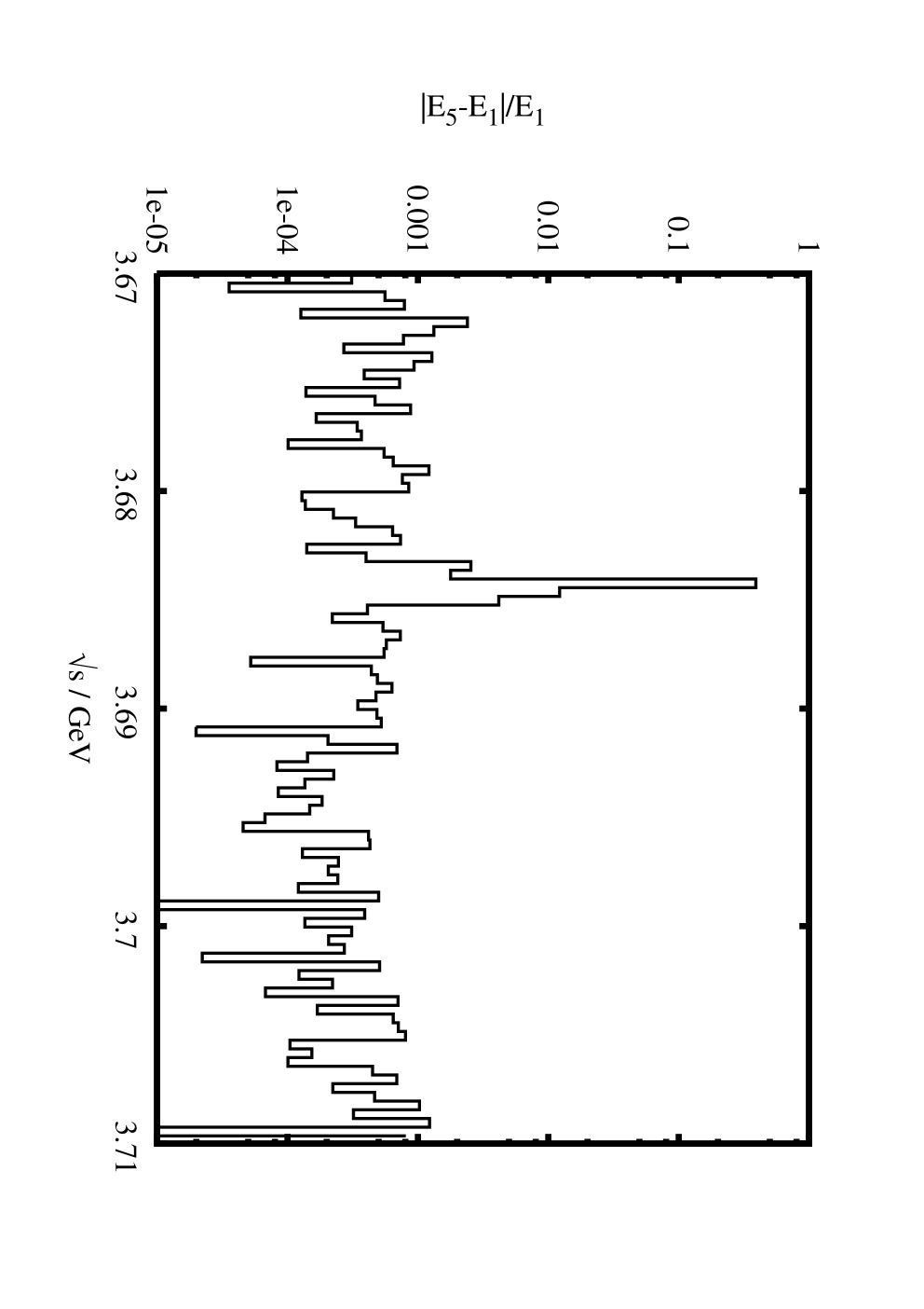
In section 4.1, we scan through the energy region using one data taking point. To check this result, five consecutive energy points are used in energy scan. The fitting error of five consecutive points scan versus the central energy point is shown in Fig. 7. This result is similar with one point scan. Their difference is also shown in Fig. 7. The difference between the two scan schemes is generally at the level of one per mille except for the points around 3.684 GeV, where the variation of error curve is rather rapidly. As to the five-point scheme, there is at least one point within the region with comparatively large error.
References
- [1] DMII Collab. (J. Jousset et al.), Phys. Rev. D 41, 1389 (1990).
- [2] Mark III Collab. (D. Coffman et al.), Phys. Rev. D 38, 2695 (1988).
- [3] M. Suzuki, Phys. Rev. D 60, 051501 (1999).
- [4] G. López, M.J.L. Lucio and J. Pestieau, hep-ph/9902300
- [5] L. Köpke and N. Wermes, Phys. Rep. 174, 67 (1989).
- [6] R. Baldini et al., Phys. Lett. B 444, 111 (1998).
- [7] M. Suzuki, Phys. Rev. D 63, 054021 (2001).
- [8] J.M. Gérard and J. Weyers, Phys. Lett. B 462, 324 (1999).
- [9] C.Z. Yuan, P. Wang and X.H. Mo, Phys. Lett. B 567, 73 (2003).
- [10] P. Wang, C.Z. Yuan and X.H. Mo, Phys. Rev. D 69, 057502 (2004).
- [11] BES Collab. (J.Z. Bai et al.), Phys. Rev. Lett. 91, 052001 (2004).
- [12] P. Wang, C.Z. Yuan and X.H. Mo, Phys. Lett. B 574, 41 (2003).
- [13] P. Wang, X.H. Mo and C.Z. Yuan, Int. J. Mod. Phys. A 21, 5163 (2006).
- [14] BESII Collab. (M. Ablikim et al.), Phys. Rev. D 70, 077101 (2004).
- [15] Q.Qin et al., Status and Performance of BEPCII, IPAC-2010-WEXMH01, May 2010.
- [16] The BESIII Collaboration, Design and Construction of the BESIII Detector, arXiv: 0911.4960, 2009.
- [17] Z.Y. Wang, G. Li, K. Zhu, et al., total number, BAM-00003; H.X. Yang, B.X. Zhang, X.T. Liao, et al., Determination of total number, BAM-00011; Lili Jiang, et al., Measurements of the luminosity at 3.773 GeV and 3.650 GeV, BAM-00037.
- [18] Y.K. Wang, X.H. Mo, C.Z. Yuan, et al., Nucl. Instr. Meth. A 583, 479 (2007).
- [19] Y.K. Wang, J.Y. Zhang, X.H. Mo, C.Z. Yuan, et al., Chinese Physics C 33, 501 (2009).
- [20] P. Wang, X.H. Mo and C.Z. Yuan, Phys. Lett. B 557, 192 (2003).
- [21] E.A. Kuraev and V.S. Fadin, Sov. J. Nucl. Phys. 41, 466-472 (1985).
- [22] G. Altarelli and G. Martinelli, CERN 86-02, 47 (1986).
- [23] F.A. Berends, G. Burgers and W.L. Neerven, Nucl. Phys. B 297, 429 (1988); F.A. Berends, G. Burgers and W.L. Neerven, Nucl. Phys. B 304, 921 (1988).
- [24] S.Y. Lee, Accelerator Physics, 2nd edn. (FuDan University Press, Shanghai, 2006)
- [25] K. Wille, The Physics of Particle Accelerators (Oxford University Press, New York, 2000)
- [26] Particle Data Group (K. Nakamura et al.), J. Phys. G 37, 075021 (2010).
- [27] CLEO Collab. (T.K. Pedlar et al.), Phys. Rev. Lett. 95, 261803 (2005).
- [28] BES Collab. (J.Z. Bai et al.), Phys. Lett. B 550, 24-32 (2002).
- [29] CLEO Collab. (S.Dobbs et al.), Phys. Rev. D 74, 011105 (2006).
- [30] Y.S. Zhu, Probability and Statistics in Experimental Physics, 2nd edn. (Science Press, Beijing, 2006)
- [31] B.Q. Wang, X.H. Mo, et al., Chinese Physics C 35, 411 (2011).