Linear Network Code for Erasure Broadcast Channel with Feedback: Complexity and Algorithms
Abstract
This paper investigates the construction of linear network codes for broadcasting a set of data packets to a number of users. The links from the source to the users are modeled as independent erasure channels. Users are allowed to inform the source node whether a packet is received correctly via feedback channels. In order to minimize the number of packet transmissions until all users have received all packets successfully, it is necessary that a data packet, if successfully received by a user, can increase the dimension of the vector space spanned by the encoding vectors he or she has received by one. Such an encoding vector is called innovative. We prove that innovative linear network code is uniformly optimal in minimizing user download delay. On the other hand, innovative encoding vectors do not always exist. When the finite field size is strictly smaller than the number of users, the problem of determining the existence of innovative vectors is proven to be NP-complete. When the field size is larger than or equal to the number of users, innovative vectors always exist and random linear network code (RLNC) is able to find an innovative vector with high probability. While RLNC is optimal in terms of completion time, it has high decoding complexity due to the need of solving a system of linear equations. To reduce decoding time, we propose the use of sparse linear network code, since the sparsity property of encoding vectors can be exploited when solving systems of linear equations. Generating a sparsest encoding vector with large finite field size, however, is shown to be NP-hard. An approximation algorithm that guarantee the Hamming weight of a generated encoding vector to be smaller than a certain factor of the optimal value is constructed. For the binary field, a heuristic algorithm is also proposed. Our simulation results show that our proposed methods have excellent performance in completion time and outperforms RLNC in terms of decoding time. This improvement is obtained at the expense of higher encoding time and the requirement of user feedback. Comparisons with other broadcast codes have been made and numerical results show that different tradeoff can be obtained by these schemes.
Index Terms:
Erasure broadcast channel, innovative encoding vector, sparse network code, computational complexity.I Introduction
Broadcasting has been a challenging issue in telecommunications. The challenge mainly comes from how a transmitter can disseminate a common information content to all users/receivers reliably and efficiently via a broadcast channel which could be unstable and error-prone. More specifically, one of the ultimate goal of broadcasting is to provide a transmission scheme such that a common information content or a set of packets can be disseminated with minimum number of transmissions for a sender to complete the whole information content dissemination for all users. This measure is commonly called the completion time of a broadcast system.
Several classical approaches provide heuristic solutions to the above issue. With user feedback, automatic repeat request (ARQ) offers reliable retransmissions for the erased packets due to channel impairments. However, such an approach becomes inefficient when the number of users increases, as the users may have entirely distinct needs for the erased packets. Reliable broadcasting can also be achieved without user feedback by forward error correction. With the use of erasure codes, a user can reconstruct the entire set of original packets, provided that the number of erased packets is smaller than a certain threshold. However, the amount of packets that will be erased depends on the channel erasure probability, which is time-varying and hard to predict. That limits the use of erasure codes in broadcasting. To improve upon classical approaches, the approach of linear network coding [1, 2] has been shown to be a promising solution [3, 4, 5, 6].
The idea of linear network coding for broadcasting is that a transmitter broadcasts to users encoded packets that are obtained by linearly combining the original packets over the finite field . An encoding vector specifies the coefficients for the linear combination. An encoded packet together with a header which contains the corresponding encoding vector is broadcasted to all users. It is said to be innovative to a user if the corresponding encoding vector is not in the subspace spanned by the encoding vectors already received by that user. It is called innovative if it is innovative to all users who have not yet received enough packets for decoding. It is shown in [7] that an innovative packet can always be found if . Once a user receives any innovative packets, he or she can decode the original packets by Gauss-Jordan elimination. Therefore, the generation of innovative packets is vital. Clearly, if all the encoded packets are innovative, the completion time can then be minimized.
Linear network codes for broadcasting can be generated with or without feedback. LT code [8], Raptor code [9] and random linear network code (RLNC) [10] can be used without feedback. By suitably choosing design parameters, innovative packets can be generated by those coding schemes with high probability. LT code and Raptor code are generated by an optimized degree distribution. However, they are mainly designed for broadcasting a huge number of packets, and may not be good choices when the number of packets is only moderately large. With feedback, it is suggested in [7] the use of Jaggi-Sanders algorithm [11], which is a general network code generation method and is able to find innovative encoding vectors for . However, its encoding and decoding complexities are relatively high, as it is not specifically designed for the broadcast application. Therefore, some heuristics have been proposed [12, 13, 14, 15]. It is suggested in [16] that encoded packets should be instantly decodable, in the sense that a new packet can be decoded once it is available at a receiver without waiting for the complete reception of the full set of packets. However, as an instantly decodable packet to all users may not exist, the completion time is in general larger than that in a system without this extra requirement. With the idea of instantly decodability, some works focus on minimizing decoding delay, where a unit of decoding delay is defined as that an encoded packet is successfully received by a user but that packet is not innovative or not instantly decodable to him or her [17, 18, 19, 20].
The excellent performance of linear network coding to broadcast encourages researchers to consider its practicality. In fact, the decoding complexity of a linear network code is an important issue in practice. One possible way to reduce decoding complexity is to use sparse encoding vectors. This sparsity property is important, as it can be exploited in the decoding process. For example, a fast algorithm by Wiedemann for solving a system of sparse linear equations can be used [21]. If the Hamming weight of each encoding vector is at most , the complexity for solving an linear system can be reduced from using Gaussian elimination to [22]. The Wiedemann algorithm is useful when is large. When is moderate, we can implement some sparse representation of matrices, so that even if the usual Gaussian elimination is used, the number of additions and multiplications required can be reduced. For other fast methods for solving linear equations over finite fields, we refer the readers to [23, 24].
Minimizing the completion time and reducing the decoding complexity are equally important in linear network code design for erasure broadcast channel. However, the innovativeness of encoding vectors together with their sparsity has not been thoroughly studied. Given the encoding vectors which have been received by the users in a broadcast system, the generation of encoding vectors which are both sparse and innovative is a challenging problem. In this paper, we address the issue by developing a method called the Optimal Hitting Method and its approximation version, called the Greedy Hitting Method. Both of them are able to generate sparse and innovative encoding vectors for . That results in a significant reduction in decoding complexity when compared with their non-sparse counterparts. Furthermore, based on the greedy hitting method, we develop a suboptimal procedure to improve the completion time performance for , where the existence of innovative encoding vectors is not guaranteed. Simulation results show that its performance is nearly optimal.
The rest of this paper is organized as follows. We review the literature on complexity in network coding in Section II and some useful notions in complexity theory in Section III. In Section IV, the system model is introduced and the problem is formulated. In Section V, we show that innovative linear network code is uniformly optimal. In Section VI, we characterize innovative encoding vectors by a linear algebra approach and prove that the determination of the existence of an innovative vector for is NP-complete. In Section VII, the sparsity issue is considered. After showing that -sparse innovative vectors always exist if , we investigate the Sparsity problem and prove that it is NP-complete. In Section VIII, we present a systematic way to solve Max Sparsity using binary integer programming. A polynomial-time approximation algorithm is also constructed. In Section IX, some benchmark algorithms for wireless broadcast are described. In Section X, our algorithms are compared with those benchmarks by simulations. Finally, conclusions are drawn in Section XI.
II Literature on Complexity Classes of Network Coding Problems
A considerable amount of research has been done on the complexity issues in conventional coding theory (See the survey in [25] for example). For instance, it is shown in [26] and [27] that the problems of finding the weight distribution and the minimum distance of linear codes are NP-hard. The complexity issues in network coding are less well understood.
For linear network codes, Lehman and Lehman investigated the complexity of a class of network coding problems in [28], and proved that some of the problems are NP-complete. Construction of linear network codes using a technique called matrix completion is considered in [29], and the complexity class of the matrix completion problem is studied in [30]. It is shown in [31] that approximating the capacity of network coding is also a hard problem.
To minimize encoding complexity, Langberg, Sprintson and Bruck divide the nodes in a general network topology into two classes. The nodes in one class forward packets without any coding while the nodes in another class perform network coding. The problem of minimizing the number of encoding nodes is shown to be NP-complete in [32, 33].
El Rouayheb, Chaudhry and Sprintson study the complexity of a related problem called index coding problem in [34]. They consider the noiseless broadcast channel, and show that when the coefficient field is binary, the problem of minimizing the number of packet transmissions is NP-hard. A complementary version of the index coding is studied in [35]. It is shown that the complementary index coding is NP-hard, and even obtaining an approximate solution is NP-hard.
In [36], Milosavljevic et al. studies a related system. The users are interested in a common data file but only have partial knowledge of the file. By interactively sending data to each others through a noiseless broadcast channel, the users want to minimize the total amount of data sent through the channel. It is shown in [36] that the optimal rate allocations can be found in polynomial time.
In this paper, the problem setting is similar, except that the channel is modeled as an erasure broadcast channel, and we focus on the innovativeness and sparsity aspects of generating encoding vectors.
III Useful Notions in Complexity Theory
Before presenting the broadcast problem, we first define some useful notions in complexity theory, which will be used in this paper. The following definitions are taken from [39]:
Definition 1.
Let denote the set of all binary strings, and be a subset of . A function is said to solve the decision problem of if for every binary string it holds that if and only if .
Definition 2.
For a given , let denote the set of solutions for the binary string . A function is said to solve the search problem of if for every the following holds:
Note that a minimization problem can be regarded as a search problem. By definition, a minimization problem is associated with a value function . Given , the task is to find such that and is the minimum value of for all .
The following two definitions concerning reductions between two problems:
Definition 3.
For , , A polynomial-time computable function is called a Karp-reduction of to if, for every binary string , it holds that if and only if .
Definition 4.
For , , a pair of polynomial-time computable functions,
is called a Levin-reduction of to if the function is a Karp-reduction of to , and for every and it holds that .
Detailed explanations of the above concepts can be found in [39].
IV System Model and Problem Formulation
Consider a single-hop wireless broadcast system, in which there are one source and users. The source wants to send data packets to all the users. We view each packet as a symbol from an alphabet set of size . In other words, the source wants to broadcast symbols, . We assume that they are independent random variables, each of which is drawn uniformly at random from .
We model the transmission as a time-slotted broadcast erasure channel. In time slot , a symbol is transmitted by the source. The channel output observed by user , denoted by , is either the same as or equal to a special erasure symbol . A time slot is called a non-erasure slot of user at time if , and is called an erasure slot of user otherwise. The channel dynamics is modeled by a stochastic sequence,
where equals one if or zero if . Assume that ’s are all independent of the source symbols . For , we let be the number of non-erasure slots of user in the first time slots. We let be the truncated sequence obtained from by preserving the random variables in the first time slots. After every slot , user broadcasts via a control channel without delay and error. We assume that after time , the source and all users have the knowledge of .
Define . An broadcast code is defined by encoding functions
| (1) |
and decoding functions
| (2) |
where and .
Given a broadcast code and a realization of the channel dynamics , user is said to have download delay if it is the smallest value of such that decoding is successful, that is,
| (3) |
If decoding is never successful, then we let the download delay be infinity.
The following result gives a lower bound of the download delay of each user:
Theorem 1.
Given any broadcast code and any channel realization , we have for all such that , for all .
Proof.
Consider a time index , where . Let be the indices of time slots at which user experiences no erasure, and let . Note that
Therefore, the probability that the decoding condition in (3) holds must be strictly less than one. In other words, the download delay of user , , must be strictly greater than , for all ’s. ∎
Definition 5.
An broadcast code is said to be uniformly optimal if for any channel realization and ,
| (4) |
If the minimum does not exist, we define it as infinity.
The existence of uniformly optimal broadcast code will be investigated in the next two sections.
V Linear Network Code
In this paper, we focus on the use of linear network code. The alphabet set is identified with the finite field of size , for some prime power . We define linear network code formally below:
Definition 6.
An broadcast code is said to be a linear network code if its encoding functions can be expressed as a linear function of the source packets:
| (5) |
where are determined by , and the addition and multiplication operations are defined over .
The vector , as expressed in (5), is called the encoding vector of the packet transmitted in slot . Throughout this paper, all vectors are assumed to be column vectors, and we use parenthesis and commas when its components are listed horizontally.
For practical applications, the transmitter can put the encoding vector in the header of the encoded packet. While that incurs some transmission overhead, it can relax the requirement specified in the previous section that every user can listen to the feedback information from all other users. In other words, the decoding function of user in (2) can be changed to
| (6) |
assuming that the decoder knows the encoding vectors of its received packets.
The support of the vector , denoted by , is the set of indices of the non-zero components in , i.e.,
The Hamming weight of is defined as the cardinality of . An encoding vector that has Hamming weight less than or equal to is said to be -sparse.
Note that a transmitted packet brings new information to a user if and only if its entropy conditioned on the perviously received packets by that user is greater than zero, or equivalently, the new packet is not a function of the previously received packet. In linear algebraic terms, the condition is that the encoding vector of the new packet does not lie within the span of all previously received encoding vectors of that user. We say that such an encoding vector is innovative to that user. An encoding vector that is innovative to all users is simply said to be innovative.
Suppose that user , for , has already received packets whose encoding vectors are linearly independent. Let be the encoding matrix of user , whose rows are the transposes of the encoding vectors. Without loss of generality, we assume that , for otherwise user can decode the file successfully and can be omitted from our consideration. A vector is innovative if it does not belong to the row space of for any . Given encoding matrices , the set of all innovative encoding vectors, , is given by
| (7) |
Definition 7.
A linear network code is said to be innovative if for any channel realization , its encoded packet at time is innovative to all users who have not successfully decoded the source packets yet, that is, those users with indices in .
Theorem 2.
Innovative linear network codes are uniformly optimal.
Proof.
With an innovative linear network code, by definition, the packets received by a user who has not successfully decoded all the source packets must all be linearly independent. Therefore, she is able to decode the source packets once she has experienced non-erasure slots. In other words, (4) holds for all users. Hence the code is uniformly optimal. ∎
In the next section, we will show that innovative linear network codes exist when .
VI The Innovative Encoding Vector Problem
The existence of innovative linear network code is equivalent to the non-emptiness of the set of encoding vectors as defined in (7). It was shown in [7] that is non-empty if the finite field size, , is larger than or equal to the number of users, . We present a proof below for the sake of completeness. We begin with a simple lemma, which will be used again in a later section.
Lemma 3.
Let be finite subsets of a universal set . If and contain a common element, then
Proof.
Suppose for all . Let be the set for . By applying the union bound,
This implies that
As by hypothesis, we obtain the inequality in the lemma. ∎
Theorem 4 ([7]).
If and the rank of is strictly less than for all ’s, then is non-empty.
Proof.
For , let be the row space of . The subspace consists of the encoding vectors which are not innovative to user . Obviously the zero vector is a common vector of these subspaces. By Lemma 3, the union of these subspaces contains strictly less than vectors. Since , we have . Therefore there exists at least one encoding vector which is innovative to all users. ∎
The condition in Theorem 4 cannot be improved in general. In Appendix A we construct examples with no innovative encoding vector for .
The set of innovative encoding vectors, , can be characterized by the orthogonal complements of the row spaces of ’s, which is also known as the null spaces of ’s. For , let be the row space of . Denote the orthogonal complement of by ,
where is the inner product of and . We will use the fact from linear algebra that a vector is in if and only if for all . Let be an matrix whose rows form a basis of . To see whether a vector is in , it amounts to checking the condition ; if , then , and vice versa.
There are many different choices for the basis of the orthogonal complement . We can obtain one such choice via the reduced row-echelon form (RREF) of . Suppose we have obtained the RREF of by elementary row operations. By appropriately permutating the columns of , we can write in the following form:
| (8) |
where is the identity matrix, is an matrix over , and is an permutation matrix11 1 Recall that a permutation matrix is a square zero-one matrix so that each column and each row contain exactly one “1”.. We can take
| (9) |
The superscript T represents the transpose operator. It is straightforward to verify that the product of the matrix in (8) and is a zero matrix. Hence, the row vectors in belong to the orthogonal complement . Since contains a permutation of as one of its submatrices, the rows of are linearly independent. As , we conclude that the rows of form a basis of .
In Appendix B, we give another way of computing a basis of , which is suitable for incremental processing.
The following simple result characterizes the set of innovative encoding vectors, :
Lemma 5.
Given , an encoding vector belongs to if and only if for all ’s.
Proof.
If , then is not in and therefore, is innovative to user . It is innovative if for all ’s.
Conversely, if for some , then is in , and hence is not innovative to user . Therefore, . ∎
When the underlying finite field size is small, innovative encoding vectors may not exist. For further investigation of the existence of innovative encoding vectors, we formulate the following decision problem:
Problem:
Instance: matrices, , over , each of which has columns.
Question: Is there an -dimensional vector over which does not belong to the row space of for ?
We can assume without loss of generality that all the matrices to in are not full-rank. Also, we know from Theorem 4 that the answer to is always Yes if . The following result shows that the problem is NP-complete for .
Theorem 6.
is NP-complete.
Proof.
The idea is to Karp-reduce the 3- problem, well-known to be NP-complete [37], to the problem. Recall that the 3- problem is a Boolean satisfiability problem, whose instance is a Boolean expression written in conjunctive normal form with three variables per clause (3-), and the question is to decide if there is some assignment of True and False vaules to the variables such that the given Boolean expression has a True value.
Let be a given Boolean expression with variables , and clauses in 3-. We want to construct a Karp-reduction from the 3- problem to the problem with packets and users.
For the -th clause (), we first construct a matrix . If the -th literal () in the -th clause is , then let the -th component in the -th row of be one, and the other components be all zero. Otherwise, if the -th literal in the -th clause is , then let the -th and the -st component in the -th row of be both one, and the remaining components be all zero. Let be a matrix whose rows form a basis of the orthogonal complement of the row space of . We will use the fact that a vector is in the row space of if and only if .
Consider an example with Boolean variables. From the clause , we get
It can be verified that each row in is orthogonal to the rows in , i.e., the row space of is the orthogonal complement of the row space of .
For the extra user, user , let be the matrix , where stands for the all-zero vector. The problem reduction can be done in polynomial time.
Let be a Boolean vector and define . Note that any solution to a given 3- problem instance would cause the product a non-zero vector for . By Lemma 5, is not in the row space of for all . Hence is also a solution to the derived problem.
Conversely, any solution to the derived problem also yields a solution to the original 3- problem as well. Let be a solution to the derived problem. Note that we must have because of . Let be an index between 1 and . Since is not in the row space of , the product is a non-zero vector. Hence, if we assign True to if and False to if , for , then the -th clause will have a True value. Since this is true for all , the whole Boolean expression also has a True value.
The problem is clearly in NP, since it is efficiently verifiable. Hence it is NP-complete. ∎
The above proof can be extended to the following more general result:
Theorem 7.
For any prime power , the problem is NP-complete.
Proof.
The reduction from 3- to is the same as before, except with the following changes:
- 1.
In the derived problem, users. In other words, there are more users than that in the previous proof.
- 2.
For , is defined the same as before except that when the -th literal in the -th clause is , let the -th component be (rather than 1).
- 3.
For , let be matrices whose -th components are distinct elements in and the (+1)-st components are all equal to . Let these matrices be ’s for .
The forward part is the same as before, so we only need to consider the converse part. Let be a solution to the derived problem. Same as before, we must have because of . Since a non-zero scalar multiplication of remains to be a solution to the derived problem, without loss of generality, we can assume that . Due to the extra users, for , we must have or 1, for otherwise must be zero for some . (More precisely, one and only one of these vectors is zero.) The rest of the proof then follows the same argument as in Theorem 6. ∎
Note that in the formulation of the values of and are arbitrary. The above result shows that it is NP-complete. With the restriction of , becomes trivial to solve, as shown by Theorem 4.
Apart from the problem of existence of an innovative vector, it is also of interest in finding an -dimensional encoding vector that is innovative to as many users as possible. We state the optimization problem as follows:
Problem: -
Instance: matrices over , , and each matrix has columns.
Objective: Find an -dimensional vector over such that the number of users to whom is innovative is maximized.
The following result shows the hardness of finding approximate solution to -:
Theorem 8.
For , there is no approximation algorithm for - with an approximation guarantee of , assuming , where is a positive constant.
Proof.
Given a Boolean expression in the 3- form, the problem of maximizing the number of clauses that have TRUE values is commonly called the -3- problem. Consider the same reduction described in the proof of Theorem 6. It is clear that the number of clauses that have True values under a given Boolean vector is the same as the number of users to whom is innovative, excluding user . Therefore, the reduction is a gap-preserving reduction from -3- to -. The statement then follows from [38, Corollary 29.8]. ∎
VII The Sparsity Problem
Decoding complexity is one of the critical issues that could determine the practicality of linear network coding in broadcast erasure channels. One way to reduce the decoding complexity is to generate sparse encoding vectors and apply a decoding algorithm that exploits the sparsity of encoding vectors at receivers. In this section, we focus on the sparsity issues of innovative encoding vectors.
VII-A Existence of -sparse innovative vector
In the previous section, it is found that innovative vectors always exist if . In fact, we can prove a stronger statement that -sparse innovative vectors always exist under the same condition.
Lemma 9.
For , let be a non-zero linear polynomials in variables
where the coefficients are elements in . If , we can always find a vector such that for all .
We first give a combinatorial proof:
Proof.
For , let be the set of vectors in satisfying . The set is a subspace of dimension . By Lemma 3, the cardinality of the union of these subspaces is strictly less than elements, which in turn is less than or equal to the cardinality of the whole space . Thus there exists at least one vector in such that for all . ∎
Now we give an alternative proof of Lemma 9, which is algorithmic and constructive:
Proof.
Let , where , be the index set such that if and only if . Since none of the linear polynomials ’s are identically zero, the union is equal to . We distinguish two cases:
Case 1: for some . We can simply let and for .
Case 2: for all . We assign values to the variables iteratively. Suppose we have already assign to the first variables. We note that is a linear equation in a single variable , and thus have only one solution. As , the number of elements in which satisfy for some is strictly less than . There must exist such that
for all . Upon termination, it is guaranteed that for all . ∎
We call the method in the proof of Lemma 9 the Sequential Assignment (SA) algorithm. Its computational complexity in terms of number of multiplications/divisions over is analyzed as follows: In this algorithm, there are iterations. In each iteration, we need to find an element in that is not a root of any of these equations. Consider the -th iteration. For the -th equation, we need to compute and add it to the accumulated sum , which is stored for the next iteration. The root of this equation can then be obtained by a division. Therefore, the total complexity of SA is .
Example 1.
Let
be linear polynomials over . We apply the SA algorithm to find an assignment of such that , and are all non-zero. First of all, the three index sets are , , and . None of them has cardinality three. We proceed as described in the second case. We assign an arbitrary non-zero value to , say , and we can check that , , .
Next, we want to find such that
It turns out that the only choice for is . After is fixed, we search for such that
The only choice for is . Finally, we check the values of , and evaluated at as follows:
Lemma 9 can be used to establish the following result:
Theorem 10.
If , there exists a -sparse encoding vector in .
Proof.
For , let be an arbitrary row vector in , and let be an arbitrary index such that the -th component of is non-zero. Form a new index set that consists of all ’s. The cardinality of may be less than since the ’s may not be distinct. Let be a truncated vector of , which consists of only the components of whose indices are in . Its dimension is equal to .
Now we show that there exists a vector such that the -th component of is equal to zero if . If the -th component of is zero for all , then the inner product of and is the same as the inner product of and . According to Lemma 5, is in if for all ’s. By Lemma 9, we can find such a vector if . Clearly, such a vector has as its support, and is hence -sparse. ∎
The above result shows that if , the minimum Hamming weight of innovative vectors is bounded above by . This upper bound cannot be further reduced as the following example shows:
Example 2.
Consider a broadcast system of users and packets, where . Suppose that user has received a set of uncoded packets . Here we regard as a subset of . Furthermore, suppose that the complement of the ’s are mutually disjoint, i.e., for . In such a scenario, an innovative packet must be a linear combination of at least packets. For example, let and . If the encoding matrices of the three users are
then an innovative encoding vector must have Hamming weight at least 3. For instance and are innovative, but no vector with Hamming weight 2 or less is innovative.
VII-B Sparsest Innovative Vectors
Theorem 10 shows that we can always find a -sparse innovative vector if . It serves as an upper bound on the minimum Hamming weight of innovative vectors. To further reduce the decoding complexity, it is natural to consider the issue of finding the sparsest innovative encoding vector for given ’s. In other words, we want to find a vector in that has the minimum Hamming weight for the case where . We call this algorithmic problem Sparsity. We state its decision version formally as follows:
Problem: Sparsity
Instance: A positive integer and matrices with columns, , over , where .
Question: Is there a vector with Hamming weight less than or equal to ?
We have already proven that the answer is always Yes if . We are interested in the case where .
Given all ’s, we can find a basis ’s of their corresponding null spaces by the method mentioned in Section VI. For , let be the -th row of . We define
| (10) |
where denotes the logical-OR operator applied component-wise to the vectors, with each non-zero component being regarded as a “1”. In other words, the -th component of is one if and only if the -th column of is nonzero. We define as the matrix whose -th row is equal to . Note that is a binary matrix and has no zero rows. For a matrix and a subset of the column indices of , let be the submatrix of , whose columns are chosen according to . We need the following lemma:
Lemma 11.
Let be an index set and . There exists an encoding vector over with if and only if has no zero rows.
Proof.
If has no zero rows, then for all ’s. Furthermore, for all ’s, there must exist for some . By Lemma 9, we can find such that for all ’s. Let the components of whose indices do not belong to be zero. Then by Lemma 5, .
Conversely, if is an innovative vector with for , then cannot have zero rows, for if row of is a zero vector, then is a zero matrix and the -th inequality in Lemma 5 cannot hold. ∎
The NP-completeness of Sparsity can be established by reducing the hitting set problem, HittingSet, to Sparsity. Recall that a problem instance of HittingSet consists of a collection of subsets of a finite set . A hitting set for is a subset of such that it contains at least one element from each subset in . The decision version of this problem is to determine whether we can find a hitting set with cardinality less than or equal to a given value.
Problem: HittingSet
Instance: A finite set , a collection of subsets of and an integer .
Question: Is there a subset with cardinality less than or equal to such that for each we have ?
It is well known that HittingSet is NP-complete [37].
Example 3.
Let ,
and . We can check that is a hitting set of size .
Theorem 12.
Sparsity is NP-complete.
Proof.
We are going to reduce HittingSet to an instance of Sparsity via a Karp-reduction. Let the cardinality of be . Label the elements of by . We define , where is the number of non-empty subsets in . For , form an -vector with its -th component equal to one if is in and zero otherwise, i.e., is the characteristic vector of . Note that and . These ’s correspond to the degenerate form of ’s in Lemma 5 with only one row in . Let be the encoding matrix of user , whose row space is the null space of and be the innovative vector set defined in (7). In other words, any instance of HittingSet can be represented as an instance of Sparsity in polynomial time.
It remains to show that there exists a hitting set for with if and only if there exists an with Hamming weight . Given the ’s obtained via the above reduction, suppose there exists with . By Lemma 5, we must have for all ’s, which implies for all ’s. The set is therefore a hitting set for the given instance. Conversely, given a hitting set for with , by definition for all ’s. Therefore, has no zero rows. By Lemma 11, there exists an such that . Hence, .
As Sparsity is verifiable in polynomial time, Sparsity is in NP. Hence it is NP-complete. ∎
Now we define the optimization version of Sparsity as follows:
Problem: Max Sparsity
Instance: A positive integer and matrices with columns, , over , where .
Objective: Find a vector with minimum Hamming weight.
We call the minimum Hamming weight among all innovative vectors the sparsity number, and denote it by . It is easy to see that if a polynomial-time algorithm can be found for solving the optimization version of Sparsity, then that algorithm can be used for solving the decision version of Sparsity in polynomial time as well. Therefore, Max Sparsity is NP-hard.
On the other hand, if is held fixed, meaning that the problem size grows only with , then there exists algorithm whose complexity grows polynomially in to solve Max Sparsity. It is proven in [40] and Section VII-A that a -sparse vector exists in , if . By listing all vectors in with Hamming weight less than or equal to , we can use Lemma 5 to check whether each of them is in . For each -sparse encoding vector, we compute the matrix product for . Each matrix product takes finite field operations. The total number of finite field operations for each candidate is . After checking all -sparse encoding vectors, we can then find one with minimum Hamming weight. The number of non-zero vectors in with Hamming weight no more than is equal to . For fixed and , the summation is dominated by the largest term when is large, which is of order . The brute-force method can solve the problem with time complexity of . As is held fixed, Max Sparsity can be solved in polynomial time in .
Let Min HittingSet be the minimization version of the hitting set problem, in which we want to find a hitting set with minimum cardinality. The next result shows that Max Sparsity can be solved via Min HittingSet based on the concept of Levin-reduction.
Theorem 13.
Max Sparsity can be Levin-reduced to Min HittingSet.
Proof.
Given an instance of Max Sparsity, we determine as in (10) for . Then we form the following instance of Min HittingSet:
Let be a solution to the above instance. Then has no zero rows. By Lemma 11, there exists a vector over with . Such a vector can be found by the SA algorithm in polynomial time.
We claim that there does not exist with Hamming weight , and thus must equal . Suppose there exists such a vector . Lemma 11 implies that has no zero rows, which in turn implies that for all ’s. Then would be a hitting set with cardinality strictly less than . A contradiction.
The proof is completed by matching the relevant entities and procedures with those in Definition 4. Note that the transformation of a given instance of Max Sparsity to an instance of Min HittingSet in essence corresponds to the mapping . A solution to an instance of Min HittingSet, , corresponds to . Obtaining from by the SA algorithm corresponds to the mapping . ∎
VIII Network Coding Algorithms
In this section, we present algorithms that generate sparse innovative encoding vectors for . While for the binary case (i.e., ), finding an innovative encoding vector may not always be possible, a modification of the algorithm is also proposed for handling it.
VIII-A The Optimal Hitting Method
For , we generate a sparest innovative vector in two steps. First we find an index set with minimum cardinality, which determines the support of the innovative encoding vector. This is accomplished by solving the hitting set problem. Once is found, the non-zero entries in the vector can be obtained by the SA algorithm.
The hitting set problem can be solved exactly by binary integer programming (BIP), formulated as follows:
subject to
where
is a binary matrix, is an -dimensional binary vector, the vector is the -dimensional all-one vector, and the inequality sign is applied component-wise.
To solve the above problem, we can apply any algorithm for solving BIP in general, for example the cutting plane method. We refer the readers to [41] for more details on BIP.
Example 4.
Let , and , and the orthogonal complements of , and be given respectively by the row spaces of
The vectors , for , are
The corresponding instance of Min HittingSet is:
The solution to both Max Sparsity and Min HittingSet can be obtained by solving the following BIP:
subject to
One optimal solution is and . That means, the sparsity number, , is equal to two and . Furthermore, according to Lemma 11, a 2-sparse innovative encoding vector can be found, for example, by the SA algorithm.
We call the above procedure for generating an innovative vector with minimum Hamming weight the Optimal Hitting (OH) method. We summarize the algorithm as follows:
The Optimal Hitting method (OH):
Input: For , full-rank matrix over , where and .
Output: with minimum Hamming weight.
Step 0: Initialize as the zero vector.
Step 1: For , obtain a basis of the null space of . Let be the matrix over whose -th row is the -th vector in the basis.
Step 2: For , let be the component-wise logical-OR operations to the row vectors of . (Each non-zero component of is regarded as “1” when taking the logical-OR operation.)
Step 3: Solve the corresponding Min HittingSet as shown in Theorem 13 and return .
Step 4: For , choose a row vector from , say , such that .
Step 5: Determine such that for , by the SA algorithm.
Example 4 (continued). We solve the hitting set problem in Step 3 and obtain . Hence, . In Step 4, we choose
In Step 5, we obtain and . Note that both and are not equal to 3. We next set , and choose such that
We can choose to satisfy these two inequalities simultaneously. The vector is an innovative encoding vector of minimum Hamming weight.
VIII-B The Greedy Hitting Method
Step 3 in the OH method requires solving an NP-hard problem. Therefore, some computationally efficient heuristics should be considered in practice. It is well known that Min HittingSet can be solved approximately by the following greedy approach [42]:
- •
Repeat until all sets of are hit:
- –
Pick the element that hits the largest number of sets that have not been hit yet.
- –
In Step 3 of the OH method, the above greedy algorithm can be used to find approximate solutions. We call this modification the Greedy Hitting (GH) method.
Theorem 14.
The GH method is an factor approximation algorithm for Max Sparsity, where is the -th harmonic number, defined as .
Proof.
It is well known that the hitting set problem is just a reformulation of the set covering problem. Therefore, the greedy algorithm is an factor approximation algorithm for Min HittingSet, as well as for the set covering problem [38]. As shown in Theorem 13, Max Sparsity can be reduced to Min HittingSet, and the sparsity number is equal to the cardinality of the minimum hitting set. Hence, GH is also an factor approximation algorithm for Max Sparsity. ∎
Now we analyze the computational complexity of the proposed OH and GH methods. For the OH method, the computation of each can be reduced to the computation of the RREF of , which takes arithmetic operations. However, if the encoding vectors are -sparse, we can adopt the dual-basis approach in obtaining as in Appendix B, and guarantee that each can be obtained in times. The computational complexity of Step 1 is thus . Step 2 involves operations. In step 3, the Min HittingSet problem shown in Theorem 13 has a complexity of [43]. Step 4 requires operations. Step 5 involves the SA algorithm, which has a complexity of . Since , the overall complexity of OH is . The only difference between OH and GH is that GH uses a greedy algorithm to approximate the Min HittingSet problem in Step 3. The greedy algorithm takes operations. Therefore, the overall complexity of GH is .
VIII-C Solving Binary Equation Set for
The last step of the GH method involves solving a set of linear inequalities over . However when , solving a linear inequality of the form is equivalent to solving the linear equation . Based on this fact, we now propose a procedure which is called Solving Binary Equation Set (SBES), which modifies the SA algorithm so that it is applicable to the case where . Note that the same idea can be applied to cases where is a prime power satisfying .
The heuristic is as follows. We want to find such that , where is the coefficient matrix of the system of linear equations. The system may be inconsistent and has no solution. Nevertheless, we can disregard some equations and guarantee that at least equations are satisfied.
Solving Binary Equation Set Procedure (SBES):
Input: A matrix over and , where .
Output: with support in .
Step 0: Let be the zero vector.
Step 1: Delete columns of whose column indices are not in . Augment the resulting matrix by adding a -dimensional all-one column vector to the right-hand side. Let the resulting matrix be denoted by .
Step 2: Compute the row echelon form (REF) of and call it .
Step 3: Delete all zero rows in and any row in if it has a single “1” in the -th entry. The resulting matrix is called . Let the number of pivots in be , and let , be the column indices of the pivot in listed in ascending order.
Step 4: Execute elementary row operations in so that is transformed into its row-reduced echelon form.
Step 5: Set the variables associated with the non-pivot columns to zero. For , assign the value of the -th entry of the last column in .
Step 6: Assign values to the components of such that , and if .
When applying the GH method to the case where , we replace the SA algorithm in Step 5 of the GH method by the SBES procedure. We call this modification GH with SBES.
Example 5.
Consider , , , and
| (11) |
We extract the first and third rows of and augment it by the all-one column vector, ,
In Step 2, we compute the REF of
The last row is an all-zero row, representing a redundant equation. The second last row contains a one in the third component, and zero elsewhere, implying that the original system of linear equations cannot be solved. In order to get a heuristic solution, we relax the system by deleting that row, and obtain
We have and in Step 3. The matrix is already in its RREF. By Step 5, and . Finally, we set , and . As a result, equals and is innovative to all except the last user.
In the above example, an innovative vector does exist, but GH with SBES fails to find it. The main reason is that the hitting set subproblem is formulated for the case where . When is small, there is no guarantee that a non-empty must consist of a vector with support restricted in . Indeed, we will skip the greedy hitting procedure and simply let be the index set of all packets, i.e., , then it is easy to check that with the same input, the SBES procedure returns , which is an innovative vector to all users. We call this modification Full Hitting (FH) with SBES, for the reason that the hitting set is chosen as the full index set of the packets. In general, FH with SBES produces encoding vectors that are innovative to more users than GH with SBES, at the expense of higher Hamming weights. Note that the encoding vectors generated by GH with the SBES procedure may not be innovative when . They are still innovative, however, to a fraction of the users.
Now we analyze the computational complexity of FH with SBES and GH with SBES. The SBES procedure is indeed the Gauss-Jordan elimination. So the complexity of SBES is . The only difference between GH method and GH with SBES is that GH with SBES uses SBES method in the last step, instead of the SA algorithm. Therefore, the total complexity of GH with SBES is . For FH with SBES, compared with GH with SBES, it skips the greedy hitting procedure which has a complexity of . Since , the overall complexity of FH with SBES is also .
IX Benchmarks for Comparison
In this section, we describe four existing linear broadcast codes, which will be used for comparison. They are LT code[8], Chunked Code[46], Random Linear Network Code (RLNC), and Instantly Decodeable Network Code (IDNC)[47]. Their encoding and decoding complexities will also be presented.
IX-A Code Descriptions
When LT code is used, the base station repeatedly broadcasts encoded packets to all users until they have decoded all the source packets. The encoding vectors are generated as follows. The base station first randomly picks a degree value, , according to the Robust Soliton distribution (see Definition 11, [8]). It then selects source packets uniformly at random and generates an encoded packet by adding them over . A belief propagation decoder is used for decoding. For more details about the LT code, we refer the readers to [8].
RLNC can be used with two transmission phase. In the systematic phase, the base station broadcasts each source packet once. In the retransmission phase, it repeatedly broadcasts encoded packets generated over to all users until they have decoded all the source packets. Gaussian elimination is used for decoding. A user sends an acknowledgement to the base station after it has decoded all the source packets.
Chunked Code is an extension of RLNC. It divides the broadcast packets into disjoint chunks with packets per chunk. For simplicity, we assume divides . At each time slot, the base station first picks a chunk uniformly at random. Then, it generates an encoded packet by linearly combining the packets in the selected chunk with coefficients drawn from . As a result, all the encoding vectors are -sparse. A user can decode a chunk as long as it has received linearly independent encoded packets which are generated from that chunk. Gaussian elimination is used for decoding. A user sends an acknowledgement to the base station after it has decoded all the source packets.
IDNC has many different variations. We consider the Maximum Weight Vertex Search (MWVS) algorithm proposed in [47]. The broadcast is divided into two phases, the systematic phase and the retransmission phase. In the systematic phase, each source packet is broadcast to all users once. At each time slot of the retransmission phase, the base station generates an encoded packet using MWVS, and broadcasts it to all users. Each user sends a feedback to the base station after receiving the packet. Then the base station generates a new encoded packet based on the updated feedback. Such a procedure is repeated until all users have decoded all the source packets. The encoded packets are generated as follows. After the systematic phase, if the -th user has not received the -th source packet, a vertex will be defined. Two vertices, say and , are connected if
- 1.
and ; or
- 2.
, , the -th user has the -th packet and the -th user has the -th packet.
By doing so, a graph , called the IDNC graph, is constructed. Its adjacency matrix is defined in the usual way, that is, if vertex is connected to vertex , the element will be set to 1, otherwise 0. Then, define the vertex weight for each vertex as:
| (12) |
where is the erasure probability22 2 In calculating the vertex weight, it was assumed that the transmission from the base station to user experiences independent erasures in different time slots, each with probability of the channel from the base station to user , and is the number of source packets not yet received by the -th user. The vertex with the maximal weight will then be determined and added to an initially empty set, . The following iterative procedure will then be repeatedly performed:
- 1.
Let .
- 2.
Let be the subgraph induced by .
- 3.
Recompute the vertex weights using (12) with respect to the graph .
- 4.
Find the vertex in with maximal weight and adds it into .
The above procedure is repeated until no more vertices in can be added to , which occurs when in Step 1 is found to be empty. Note that the vertices in form a clique in . An encoded packet is obtained by XORing all the packets in .
IX-B Complexity Analysis
We first consider the encoding complexity. For LT code, it first generates the degree value according to the Robust Soliton distribution. This can be done by generating a random variable uniformly distributed over and checking which interval it falls within, out of the intervals defined by the Robust Soliton distribution. Encoding is completed by randomly picking source packets and adding them together over GF(2). The overall complexity is . For RLNC, the encoding complexity is also , since it requires the generations of random coefficients, multiplications and additions, all over GF(). Chunked Code is a special case of RLNC, which applies RLNC to each chunk. Since each chunk has only packets, the encoding complexity is . For MWVS, the IDNC graph can have at most vertices. To construct the graph, it takes operations to check the connectivity for each pair of vertices. For each iteration, it takes operations to compute the vertex weight for each vertex. As aforementioned, the IDNC graph can have at most vertices, therefore the complexity of each iteration is . Since the vertex set can have at most vertices, the algorithm can run at most iterations. The overall encoding complexity of MWVS is . For more details about the algorithm, we refer the readers to [47]. As analyzed in previous sections, the encoding complexity of GH is . Since it is known that , the encoding complexity of GH is lower than that of MWVS.
Now we are going to analyze the decoding complexity. For LT code, we use belief propagation decoder for decoding. The decoding process and iterative and starts from packets with degree 1. Note that the received packets and their corresponding encoding vectors will be updated during the iterative process. In each iteration, the decoder selects a successfully received packet whose current encoding vector has Hamming weight 1. In other words, is equal to for some . Then it subtracts (over GF(2)) from each of the received packets whose -th component of the encoding vector is equal to 1. The encoding vectors of these packets are then updated accordingly. Such a procedure is repeated until all the source packets are decoded. In the worst case, only one source packet is decoded in each iteration. There will be iterations and the -th iteration requires operations. Totally, operations are needed. Therefore, the decoding complexity of LT code is . For RLNC, we assume that Gaussian elimination is used for decoding. The decoding complexity is therefore . For the Chunked Code, the decoding complexity to solve each chunk is . Totally, there are chunks. Therefore, its decoding complexity is . For GH, OH, GH with SBES, FH with SBES, since all the encoding vectors are guaranteed to be sparse, decoding algorithms for solving sparse linear system can be used [22]. The decoding complexity is . For IDNC, since has at most vertices, the encoding vector of an encoded packet cannot have Hamming weight greater than . Therefore, the decoder needs at most XOR operations to decode a source packet. Since there are totally source packets, its decoding complexity is .
The encoding and decoding complexities of these schemes are summarized in Table I. Since in general grows with , in the table, we replace all by , as we know that is always bounded above by .
[b]
| Scheme | Encoding | Decoding |
|---|---|---|
| LT Code | ||
| RLNC | ||
| Chunked Code | ||
| IDNC (using MWVS) | ||
| OH | ||
| GH | ||
| GH with SBES | ||
| FH with SBES |
X Performance Evaluation
X-A Simulation Setup
In this section, we evaluate our proposed methods via simulations. We simulate a broadcast system in which a transmitter broadcasts equal-size packets to users via erasure broadcast channels. Packet erasures are assumed to be statistically independent across users and time slots. Each user experiences packet erasure with probability . We consider both the case where the transmitter receives perfect feedback from the users and the case where each feedback channel has an erasure probability .
The whole broadcast process is divided into two phases. In the first phase, the transmitter sends all source packets one by one without coding. In the second phase, packets are encoded and transmitted until all users received enough packets for recovering all the source packets. The number of packets that have been transmitted is equal to the maximum download delay of all users. We call it the completion time of the broadcast process.
We compare the performance of our proposed codes and the benchmarks described in the previous subsection. For the LT code, we let and for the Robust Soliton distribution. For the Chunked Code, we let . For our proposed methods, OH, GH and FH, we use Gaussian elimination for decoding. The performance of each code is evaluated in four ways, namely, completion time, encoding time, Hamming weights of encoding vectors, and decoding time. The completion time, as defined above, is a network performance measure, which indicates how efficient the wireless spectrum is utilized. The encoding time reflects the computational complexity of each coding algorithm. It is measured by the CPU time each coding algorithm takes in generating an encoded packet in the second phase. The Hamming weights of the encoding vectors in the second phase are recorded, so that we can evaluate the sparsity of our codes. The decoding time reflects the computational complexity of each decoding algorithm. It is important to mobile devices that do not have very high computational speed. It consists of two parts. The first part is the CPU time that is used for checking whether an encoding vector is innovative to each user. The second part is the CPU time used for decoding computation.
The system configuration of the computer used for the simulation is shown below:
- •
Intel® CoreTM 2 Quad CPU Q9650 processor (3.00GHz)
- •
Microsoft® Windows® 7 Enterprise (64-bit) with Service Pack 1
- •
4GB of RAM
All the simulation programs are written in C programming language.
To ensure the accuracy of the measured CPU time, we specify only one CPU core for the simulation process. The priority level of the simulation process is set to the highest possible value, so that the simulation will not be interrupted by any other processes. Then we use the QueryPerformanceCounter command to measure the CPU time, which can achieve microsecond precision. In our simulation figures, each data point involves 3,000 random realizations.
X-B Simulation Results
We first evaluate the performance over with various . We let , and varying from 32 to 96. The uplink channels are assumed to be perfect, i.e., . The average completion times of all the coding schemes are shown in Fig. 1. Both OH and GH are optimal, since they always generate innovative vectors for . Compared with LT code and Chunked Code, when , they can reduce their completion times by 74% and 50%, respectively. Since can be considered sufficiently large for , encoding vectors generated by RLNC are almost always innovative. As a result, RLNC performs almost the same as OH and GH.
The simulation results of encoding time is shown in Fig. 2. Since OH, IDNC and GH need to perform some computation based on the feedback from users, they have longer encoding times than LT code, Chunked Code and RLNC. While OH has longer encoding time than IDNC, GH is able to outperform IDNC by 21% when . Although both RLNC and LT have linear encoding complexity, LT works over , which is much faster than RLNC in terms of CPU time. It can also be seen that the growth of encoding time with increasing for each scheme agrees with its encoding complexity analyzed in the previous section.


The comparisons of Hamming weight and decoding time are shown in Fig. 3 and 4, respectively. The Hamming weight of encoding vectors generated by OH and GH is comparable to that of LT code and IDNC, while much smaller than that of RLNC. The advantage of transmitting sparse encoding vectors is that the decoding time can be reduced, which is shown in Fig. 4. Fig. 4 shows that the decoding time of RLNC is much higher than those of the other schemes. In particular, compared with RLNC, both OH and GH can reduce decoding time by 97% when . Besides, the growth of decoding time with increasing for each scheme agrees with the complexity analysis in the previous section.


Next, we investigate the performance with various . We let , and varying from 5 to 200 over . The uplink channels are also assumed to be perfect. The comparison of completion time is shown in Fig. 5. OH and GH are optimal and outperforms LT code, Chunked Code and IDNC. In particular, compared with LT code, Chunked Code and IDNC, both OH and GH can reduce completion time up to 68%, 40% and 17%, respectively. The gap between the performance of IDNC and OH becomes larger as increases. The reason is that IDNC works over and cannot guarantee innovative encoding vectors when is large. The comparison of encoding time is shown in Fig. 6. It can be seen that the encoding time of IDNC grows quickly with , when compared with OH and GH; the curves for RLNC, LT code and Chunked Code are flat, since their encoding methods are independent of the number of users. All these phenomena agrees with the complexity results shown in the previous section.
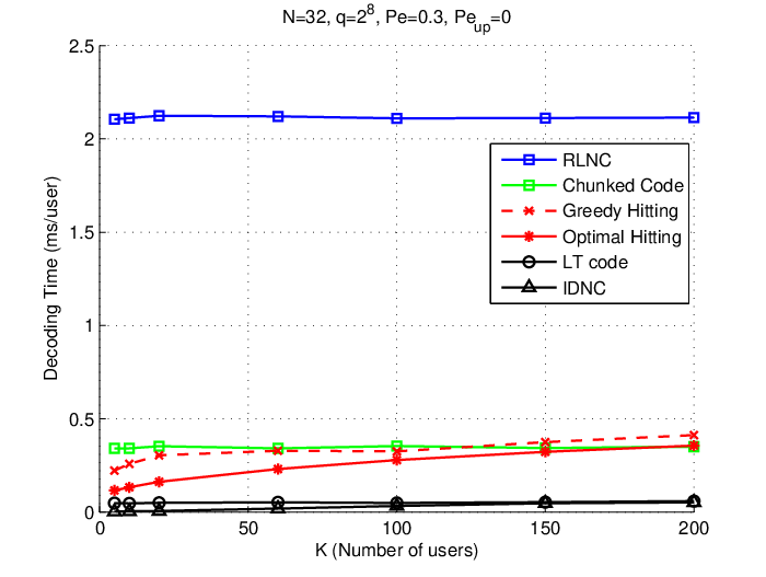
The average Hamming weights of the encoding vectors generated by RLNC, LT code and Chunked Code are constant, as shown in Fig. 7. Since the decoding time mainly depends on the Hamming weight of received encoding vectors, the decoding times of RLNC, LT code and Chunked Code keep unchanged as increases. However, the decoding times of OH, GH and IDNC slightly increase as increases, which is shown in Fig. 8. This agrees with the complexity results shown in the previous section.


To study the performance under different fading environment, we run simulations with various erasure probability . We set , and over . The erasure probability various from to . The completion times of the coding schemes are shown in Fig. 9. Since OH, GH and RLNC always transmit innovative packets, they have shorter completion times in all scenarios. The comparison of encoding times, Hamming weight and decoding times are similar to Fig. 2, 3 and 4, respectively, and are omitted here.

The performance comparison of these schemes are summarized in Table II. It is clear that there is no dominant scheme and there is a tradeoff between different performance measures. Our proposed methods, OH and GH, achieves optimal completion time like RLNC. As RLNC has very long decoding time, we design OH and GH to generate sparse encoding vectors so that the decoding time can be reduced. It is, however, at the expense of higher encoding time and user feedback.
| Scheme | Comple-tion Time | Decoding | Encoding | Feedback Required? | Field Size |
|---|---|---|---|---|---|
| LT Code | Long | Fast | Fast | No | |
| RLNC | Optimal | Very Slow | Fast | No | |
| Chunked Code | Sub-optimal | Faster than RLNC | Fast | No | |
| IDNC | Sub-optimal | Fast | Slow | Yes | |
| OH | Optimal | Faster than RLNC and GH | Slow | Yes | |
| GH | Optimal | Faster than RLNC | Slow (Faster than OH) | Yes |
Since the binary field is widely used in engineering, we also study the performance of these schemes over . In the binary field, innovative encoding vectors cannot be guaranteed. However, simulation shows that FH and GH still have shorter completion time. In particular, compared with LT, Chunked Code, IDNC and RLNC, they can reduce completion time by 77%, 53%, 15% and 5%, respectively, when .

As feedback channels in reality are not error-free, we also investigate the case where the feedback channels have erasures. In Fig. 11, we plot the completion times with , and over . It can be seen that OH and GH have longer completion times than RLNC does, but still outperforms LT code, Chunked Code and IDNC. In particular, when , compared with RLNC, OH and GH requires 15% longer completion time than RLNC, while compared with LT code, Chunked Code and IDNC, they can reduce their completion times by 73%, 30% and 20%, respectively.

XI Conclusions
In this paper, we adopt the computational approach to study the linear network code design problem for wireless broadcast systems. To minimize the completion time or to maximize the information rate, the concept of innovativeness plays an important role. We show that innovative linear network code is uniformly optimal in minimizing user download delay. While it is well known that innovative encoding vectors always exist when the finite field size, , is greater than the number of users, , we prove that the problem of determining their existence over smaller fields is NP-complete. Its corresponding maximization version is not only hard to solve, but also hard to approximate. Nevertheless, for , we propose a heuristic called FH with SBES, which is numerically shown to be nearly optimal under our simulation settings.
Sparsity of a network code is another issue we have addressed. When , we show that the minimum Hamming weight within the set of innovative vectors is bounded above by . To find a vector that achieves the minimum weight, however, is proven to be NP-hard via a reduction from the hitting set problem. An exact algorithm based on BIP is described, and a polynomial-time approximation algorithm based on the greedy approach is constructed.
The performance of our proposed algorithms has been evaluated by simulations. When , our proposed algorithm is optimal in completion time and is effective in reducing decoding time. When , our proposed algorithm is able to strike a proper balance between completion time and decoding time. Our proposed methods, however, require longer encoding time and the availability of user feedback. We believe that there is no scheme which can dominate all other schemes in all aspects. Which broadcast codes are more suitable to use depends on the specific application scenario.
Acknowledgements: The authors would like to thank Prof. Wai Ho Mow and Dr. Kin-Kwong Leung for their stimulating discussions in the early stage of this work.
Appendix A Problem instances with no Innovative Encoding Vector when
In this appendix we show that the condition in Theorem 4 cannot be relaxed.
Let be the ambient space , and consider a subspace of with dimension . Let be a basis of . For a given vector in , we let denote the the vector subspace in generated by and . We claim that we can find non-zero vectors in such that for , the sets of vectors are mutually disjoint. We can pick sequentially as follows. Firstly, we let to be any vector in . For , we let to be any vector in
| (13) |
The set in (13) is non-empty because, by the union bound, we have
If are chosen according to the above procedure, then and are disjoint for . Otherwise, if and have non-empty intersection for some , then we have
for some non-zero scalar and in and vectors and in , but this implies that
contradicting the condition in (13). For , we create an instance of the problem of finding an innovative encoding vector by defining as the matrix whose row vectors are , and . The row spaces corresponding to the matrices ’s satisfy
(i) for all .
(ii) whenever .
(iii) For , the sets are mutually disjoint.
The size of the union of is
Hence the rowspaces of ’s cover the whole vector space . Any encoding vector we pick from is not innovative to at least one user.
As an example, we consider the case and and . If the encoding matrices are
then we cannot find any innovative encoding vector.
Appendix B Incremental Method for Computing a Basis of the Null Space of a Given Matrix
In this appendix, we illustrate how to compute a basis of the null space incrementally. In the application to the broadcast system we consider in this paper, the rows of are given one by one. A row is revealed after an innovative packet is received. Given an matrix over , recall that our objective is to find a basis for the null space of . The idea is as follows. We first extend to an matrix by appending row vectors. These vectors are chosen in a way such that the resulting matrix, denoted by , is non-singular. Let be the inverse of . By the very definition of matrix inverse, the last columns of is a basis for the null space of .
We proceed by induction. The algorithm is initialized by setting . We will maintain the property that .
Suppose that the first rows of are the encoding vectors received by a user, and . We let be the -th row of and be the -th column of . When a packet arrives, we can check whether it is innovative by taking the inner product of the encoding vector of the new packet, say , with , . According to Lemma 5, it is innovative to that user if and only if one or more of such inner products are non-zero.
Consider the case that is innovative. Permute the columns of , if necessary, to ensure that . This can always be done, since cannot be orthogonal to all the last columns of . Permute the rows of accordingly, so as to ensure that .
We are going to modify by updating its -st row to . This operation can be expressed algebraically by
| (14) |
where is the column vector with the -st component equal to 1 and 0 otherwise. The matrix is a rank-one matrix, with the -st row equal to , and 0 everywhere else. The inverse of can be computed efficiently by the Sherman-Morrison formula [44] [45, p.18],
| (15) |
We have used the facts that and in the above equations. The denominator of the fraction in (15) is a non-zero scalar by construction, so that division of zero would not occur.
References
- [1] S.-Y. R. Li, R. W. Yeung, and N. Cai, “Linear network coding,” IEEE Trans. on Inf. Theory, vol. 49, no. 2, pp. 371–381, Feb. 2003.
- [2] R. Koetter and M. Médard, “An algebraic approach to network coding,” IEEE/ACM Trans. Networking, vol. 11, no. 5, pp. 782–795, Oct. 2003.
- [3] A. Eryilmaz, A. Ozdaglar, and M. Médard, “On delay performance gains from network coding,” in 40th Annual Conf. on Inf. Sci. and Systems, Princeton, Mar. 2006, pp. 864–870.
- [4] M. Ghaderi, D. Towsley, and J. Kurose, “Reliability gain of network coding in lossy wireless networks,” in IEEE Int. Conf. on Comp. Comm. (INFOCOMM ’08), Phoenix, Apr. 2008, pp. 2171–2179.
- [5] J. Heide, M. V. Pedersen, F. H. P. Fitzek, and T. Larsen, “Network coding for mobile devices – systematic binary random rateless codes,” in IEEE Int. Conf. Comm. Workshops, Dresden, Jun. 2009, pp. 1–6.
- [6] E. Drinea, C. Fragouli, and L. Keller, “Delay with newtork coding and feedback,” in Proc. IEEE Int. Symp. Inform. Theory, Seoul, Jun. 2009, pp. 844–848.
- [7] M. Durvy, C. Fragouli, and P. Thiran, “Towards reliable broadcasting using ACKs,” in Proc. IEEE Int. Symp. Inform. Theory, Nice, Jun. 2007, pp. 1156–1160.
- [8] M. Luby, “LT codes,” in Proceedings of the 43rd annual IEEE symposium on foundations of computer science, Nov. 2002, pp. 271–282.
- [9] A. Shokrollahi, “Raptor codes,” IEEE Trans. Inf. Theory, vol. 52, no. 6, pp. 2551–2567, 2006.
- [10] T. Ho, M. Médard, R. Koetter, D. Karger, M. Effros, S. Jun, and B. Leong, “A random linear network coding approach to multicast,” IEEE Trans. Inf. Theory, vol. 52, no. 10, pp. 4413–4430, Oct. 2006.
- [11] S. Jaggi, P. Sanders, P. Chou, M. Effros, S. Egner, K. Jain, and L. Tolhuizen, “Polynomial time algorithms for multicast network code construction,” IEEE Trans. Inf. Theory, vol. 51, no. 6, pp. 1973–1982, Jun. 2005.
- [12] J. K. Sundararajan, D. Shah, and M. Médard, “Online network coding for optimal throughput and delay – the three-receiver case,” in Int. Symp. on Inform. Theory and its Application (ISITA), Auckland, Dec. 08, pp. 1–6.
- [13] J. K. Sundararajan, P. Sadeghi, and M. Médard, “A feedback-based adaptive broadcast coding scheme for reducing in-order delivery delay,” in Network Coding, Theory and Application (NetCod), Lausanne, Jun. 2009, pp. 1–6.
- [14] D. Nguyen, T. Tran, T. Nguyen, and B. Bose, “Wireless broadcast using network coding,” IEEE Trans. on Veh. Tech., vol. 58, no. 2, pp. 914–925, Feb. 2009.
- [15] L. Lu, M. Xiao, M. Skoglund, L. K. Rasmussen, G. Wu, and S. Li, “Efficient network coding for wireless broadcasting,” in IEEE Wireless Comm. and networking conf. (WCNC ’10), Sydney, Apr. 2010, pp. 1–6.
- [16] S. Sorour and S. Valaee, “On minimizing broadcast completion delay for instantly decodable network coding,” in IEEE Int. Conf. Comm. (ICC ’10), May 2010, pp. 1–5.
- [17] L. Keller, E. Drinea, and C. Fragouli, “Online broadcasting with network coding,” in Proc. of the Fouth Workshop on Network Coding, theory, and applications (NetCod ’08), Hong Kong, Jan. 2008, pp. 68–73.
- [18] R. Costa, D. Munaretto, J. Widmer, and J. Barros, “Informed network coding for minimum decoding delay,” in Fifth IEEE Int. Conf. on Mobile Ad-hoc and Sensor Systems (MASS ’08), Atlanta, 2008.
- [19] P. Sadeghi, D. Traskov, and R. Koetter, “Adaptive network coding for broadcast channels,” in Fifth Workshop on Network Coding, Theory and Applications (NetCod ’08), 2009, pp. 1–6.
- [20] P. Sadeghi, R. Shams, and D. Traskov, “An optimal adaptive network coding scheme for minimizing decoding delay in broadcast erasure channel,” EURASIP J. on Wireless Comm. and Networking, vol. 2010, 2010, doi:10.1155/2010/61816.
- [21] D. H. Wiedemann, “Solving sparse linear equations over finite fields,” IEEE Trans. Inf. Theory, vol. 1, no. 32, pp. 54–62, Jan. 1986.
- [22] C. W. Sung, K. W. Shum, and H. Y. Kwan, “On the sparsity of a linear network code for broadcast systems with feedback,” in Proc. of Network Coding, Jul. 2011, pp. 1-4.
- [23] E. Kaltofen and B. D. Saunders, “On Wiedemann’s method of solving sparse linear system,” in the 9th Int. Symp. on Applied Algebra, Algebraic Algorithms and error-Correcting Codes (AAECC, T. M. H. F. Mattson and T. R. N. Rao, Eds., vol. 539, 1991.
- [24] D. Coppersmith, “Solving linear equations over GF(2): the block Lanczos algorithm,” Linear algebra and its applications, vol. 192, pp. 33–60, 1993.
- [25] A. Barg, Handbook of coding theory. Elsevier Science, 1998, vol. 1, ch. Complexity issues in coding theory, pp. 649–754.
- [26] E. R. Berlekamp, R. J. McEliece, and H. C. A. van Tilborg, “On the inherent intractability of certain coding problems,” IEEE Trans. Inf. Theory, vol. 24, no. 3, pp. 348–386, May 1978.
- [27] A. Vardy, “The intractability of computing the minimum distance of a code,” IEEE Trans. Inf. Theory, vol. 43, no. 6, pp. 1757–1766, Nov. 1997.
- [28] A. R. Lehman and E. Lehman, “Complexity classification of network information flow problems,” in Proc. of the 15th annual ACM-SIAM Symp. on Discrete algorithms (SODA), 2004, pp. 142–150.
- [29] N. J. A. Harvey, D. R. Karger, and K. Murota, “Deterministic network coding by matrix completion,” in Proc. of the 16th Annual ACM-SIAM Symp. on Discrete Algorithm (SODA), Jan. 2005, pp. 489–498.
- [30] N. J. A. Harvey, D. R. Karger, and S. Yekhanin, “The complexity of matrix completion,” in Proc. of the 17th Annual ACM-SIAM Symp. on Discrete Algorithm (SODA), Jan. 2006, pp. 1103–1111.
- [31] M. Langberg and A. Sprintson, “On the hardness of approximating the network coding capacity,” IEEE Trans. Inf. Theory, vol. 57, no. 2, pp. 1008–1014, Feb. 2011.
- [32] M. Langberg, A. Sprintson, and J. Bruck, “The encoding complexity of network coding,” IEEE Trans. Inf. Theory, vol. 52, no. 6, pp. 2386–2397, Jun. 2006.
- [33] M. Langberg, A. Sprintson, and J. Bruck, “Network coding: a computational perspective,” IEEE Trans. Inf. Theory, vol. 55, no. 1, pp. 147–157, Jan. 2009.
- [34] S. El Rouayheb, M. A. R. Chaudhry, and A. Sprintson, “On the minimum number of transmissions in single-hop wireless coding networks,” in IEEE Information theory workshop (ITW), Lake Tahoe, Sep. 2007, pp. 120–125.
- [35] M. A. R. Chauhry, Z. Asad, A. Sprintson, and M. Langberg, “On the complementary index coding problem,” in Proc. IEEE Symp. Int. on Inform. Theory, St. Petersburg, Aug. 2011, pp. 306–310.
- [36] N. Milosavljevic, S. Pawar, S. El Rouayheb, and M. Gastpar, “Optimal deterministic polynomial-time data exchange for omniscience,” arXiv:1108.6046, Aug. 2011.
- [37] M. R. Garey and D. S. Johnson, Computers and intractability: A guide to the theory of NP-completeness. W. H. Freeman and Company, 1979.
- [38] V. V. Vazirani, Approximation Algorithms. Springer, 2003.
- [39] O. Goldreich, P, NP, and NP-Completeness: The Basics of Computational Complexity. Cambridge University Press, 2010.
- [40] H. Y. Kwan, K. W. Shum, and C. W. Sung, “Generation of innovative and sparse encoding vectors for broadcast systems with feedback,” to appear in Proc. IEEE Int. Symp. Inform. Theory, St. Petersburg, Jul. 2011.
- [41] A. Schrijver, Theory of linear and integer programming. John Wiley & Son, 1986.
- [42] U. Feige, “A threshold of log for approximating set cover,” Journal of ACM 45, pp. 634–652, 1998.
- [43] L. Shi and X. Cai, “An exact fast algorithm for minimum hitting set,” in Proc. of 2010 Third Int. Joint Conf. on Computational Science and Optimization, 2010, pp. 64–67.
- [44] W. H. Press, S. A. Teukolsky, W. T. Vetterling, and B. P. Flannery, Numerical Recipe, 3rd ed. Cambridge University Press, 2007, ch. 2.7.1.
- [45] R. A. Horn and C. R. Johnson, Matrix analysis. Cambridge University Press, 1985.
- [46] Y. Li, E. Soljanin and P. Spasojevic, “Three schemes for wireless coded broadcast to heterogeneous users,” in Physical Communication, 2012, doi:10.1016/j.phycom.2012.05.003.
- [47] S. Sorour and S. Valaee, “Completion delay minimization for instantly decodable network codes,” preprint, arXiv:1201.4768, 2012.