Constructing and Classifying Fully Irreducible Outer Automorphisms of Free Groups
Abstract
The main theorem of this document emulates, in the context of theory, a mapping class group theorem (by H. Masur and J. Smillie) that determines precisely which index lists arise from pseudo-Anosov mapping classes. Since the ideal Whitehead graph gives a finer invariant in the analogous setting of a fully irreducible , we instead focus on determining which of the 21 connected, loop-free, 5-vertex graphs are ideal Whitehead graphs of ageometric, fully irreducible . Our main theorem accomplishes this by showing that there are precisely 18 graphs arising as such. We also give a method for identifying certain complications called periodic Nielsen paths, prove the existence of conveniently decomposed representatives of ageometric, fully irreducible having connected, loop-free, ()-vertex ideal Whitehead graphs, and prove a criterion for identifying representatives of ageometric, fully irreducible . The methods we use for constructing fully irreducible outer automorphisms of free groups, as well as our identification and decomposition techniques, can be used to extend our main theorem, as they are valid in any rank. Our methods of proof rely primarily on Bestvina-Feighn-Handel train track theory and the theory of attracting laminations.
1 Introduction
The main theorem of this document (Theorem 14.1) is motivated by a theorem in mapping class group theory. The mapping class group of a compact surface is the group of homotopy classes of homeomorphisms . The most common mapping classes are called pseudo-Anosov. (One characterization of a pseudo-Anosov mapping class is that some representative of a pseudo-Anosov mapping class expands and contracts a pair of transverse singular measured foliations on the surface). Because of their fundamental importance in topology and geometry, both mapping class groups and pseudo-Anosov mapping classes have been objects of extensive research. The list of singularity indices associated to a pseudo-Anosov mapping class is an important invariant of the class. (Each foliation singularity for the pair of transverse singular measured foliations has an associated index). H. Masur and J. Smillie (see [MS93]) proved precisely which lists of singularity indices arise from pseudo-Anosov mapping classes. This document is the first step to proving an analogous theorem for outer automorphism groups of free groups.
For a free group of rank , , the outer automorphism group, , consists of equivalence classes of automorphisms , where two automorphisms are equivalent when they differ by an inner automorphism, i.e. a map defined by for all . Outer automorphisms can be described geometrically as follows. Let be the -petaled rose (graph having edges and a single vertex ). Given a graph with no valence-one vertices, we can assign to a (identification of the fundamental group with the free group ) via a homotopy equivalence . We call such a graph , together with its marking , a marked graph. Each element of can be represented geometrically by a homotopy equivalence of a marked graph, where is the induced map of fundamental groups. For the proof of our analogue to the mapping class group theorem, we will focus on constructing representatives of ageometric, fully irreducible outer automorphisms with particular ideal Whitehead graphs. An ideal Whitehead graph is a strictly finer invariant than a singularity index list and encodes information about the attracting lamination for a fully irreducible outer automorphism.
There is potential for an analogue to the Masur-Smillie theorem because of deep connections between outer automorphism groups of free groups and mapping class groups of surfaces. When , we have , where denotes a genus-1 torus with a single punture. Furthermore, elements are induced by homeomorphisms of and “fully irreducible outer automorphisms” (Subsection 2.2) are induced by pseudo-Anosov homeomorphisms. While we do not have such exact correspondences for , there are still strong similarities between all of the outer automorphism groups and mapping class groups , as well as between the fully irreducible and pseudo-Anosov . In fact, some with are even still induced by homeomorphisms of a compact surface with boundary (such are called geometric).
There is a large group of mathematicians exploring the parallel properties between the groups and the groups. They have made significant progress to this affect. We use some of their definitions and machinery (including the definitions of singularities, indices, and ideal Whitehead graphs for outer automorphisms of free groups, as defined in [GJLL98] and [HM11]), in order to understand an appropriate -analogue to the Masur-Smillie theorem for mapping class groups (as described in the next section).
1.1 The Question
Let denote the sum of the singularity indices for a fully irreducible as defined in [GJLL98] and in Subsection 2.8 below. An index can in some sense be thought of as recording the number of germs of initial edge segments (directions) emanating from a vertex that are fixed by a given geometric representative of . [GJLL98] gives an inequality bounding the index sum for a fully irreducible outer automorphism , in contrast with the equality , for a pseudo-Anosov on a surface , dictated by the Poincare-Hopf Theorem. With this in mind, one can ask whether every index list who’s sum satisfies this inequality is achieved. M. Handel and L. Mosher pose the question in [HM11]:
Question 1.1.
What possible index types, which satisfy the index inequality , are achieved by a nongeometric, fully irreducible element of ?
What we present here focuses on several constructions that may eventually allow us to attack this question directly and that, in the meantime, give us a stronger result for the rank-3 case when restricting to “ageometric” fully irreducible outer automorphisms and connected, -vertex ideal Whitehead graphs with no single-vertex edges (see Theorem 14.1). For an ageometric, fully irreducible and TT representative on a rose having fixed directions at the unique vertex and no periodic Nielsen paths (PNPs), i.e. paths in such that for some , the ideal Whitehead graph is the graph with one vertex for each fixed direction of and an edge between two such vertices when there exists some and edge of such that crosses over the turn formed by the directions corresponding to the vertices.
Having vertices is maximal when we refine our search to ageometric, fully irreducible outer automorphisms and connected, loop-free graphs. We focus on ageometric, fully irreducible outer automorphisms, as they are far more common and better understood than parageometrics, the only other kind of nongeometric, fully irreducible outer automorphism (geometric outer automorphisms are induced by surface homeomorphisms, thus are already understood). We focus on connected graphs, as this allows us to only look at homotopy equivalences of roses (see Proposition 3.3).
In the mapping class group case, one only sees circular ideal Whitehead graphs, making singularity index lists the best possible invariant. However, this is not true for fully irreducible outer automorphisms. Thus, a better analogue to the Masur-Smillie theorem would record possible “ideal Whitehead graphs,” instead of just singularity indices. For an ageometric, fully irreducible , the index of a component in is simply , where is the number of vertices of the component. Ideal Whitehead graphs for outer automorphisms of free groups are defined in [HM11] and discussed in Subsection 2.8 below. In the spirit of focusing on ideal Whitehead graphs, the question we give a partial answer to in this document (see Theorem 14.1) is that also posed by L. Mosher and M. Handel in [HM11]:
Question 1.2.
Which ideal Whitehead graphs arise from ageometric, fully irreducible outer automorphisms of rank-3 free groups?
We call graphs with no single-vertex edges (i.e. no edges are loops) loop-free and a connected, ()-vertex, loop-free graph a Type (*) potential ideal Whitehead graph or Type (*) pIW graph (pIWG). The partial answer (Theorem 14.1) we give completely answers the following subquestion posed in person by L. Mosher and M. Feighn:
Question 1.3.
Which of the twenty-one five-vertex Type (*) pIW graphs are ideal Whitehead graphs for ageometric, fully irreducible ?
Theorem 1.4.
Precisely eighteen of the twenty-one five-vertex Type (*) pIW graphs are ideal Whitehead graphs for ageometric, fully irreducible .
As mentioned above, we chose to look at -vertex graphs because, with the restriction that must be ageometric and fully irreducible and the restriction that is loop-free and connected, five vertices is maximal. We focused on connected graphs as this allowed us to focus on representatives on the rose (see Proposition 3.3).
As they will be used throughout, we list now the -vertex Type (*) pIWGs.

Remark 1.5.
The -vertex Type (*) pIWGs that are not ideal Whitehead graphs for ageometric, fully irreducible are:

1.2 Outline of Document
Proposition 1.6.
Let an ageometric, fully irreducible be such that is a Type (*) pIWG. Then there exists a PNP-free, rotationless representative of a power of on the rose. Furthermore, the representative can be decomposed as a sequence of proper full folds of roses.
(The point of being rotationless is its representative fixing the periodic directions.)
The significance, for our purposes, of the proposition is its refining our search for representatives with desired ideal Whitehead graphs to those “ideally decomposed,” as in the proposition.
The next step to proving Theorem 14.1 is to define, as we do in Section 4, “lamination train track structures ” (LTT structures). We “build” or “construct” portions of desired ideal Whitehead graphs by determining “construction compositions” from smooth paths in LTT structures. “Construction compositions” are in ways analogues to Dehn twists (mapping class group elements used in pseudo-Anosov construction methods, including those of Penner in [P88]). We appropriately compose construction compositions to construct (for the Theorem 14.1 proof) the representatives of outer automorphisms with particular ideal Whitehead graphs. On the other hand, we use that LTT structures for ageometric, fully irreducible outer automorphisms are “birecurrent” to show in Proposition 5.4 that the ideal Whitehead graph of an ageometric, fully irreducible outer automorphism cannot be of a certain type. While stated in the restricted form it is used for (and we give definitions for) in this document, what the Proposition 5.4 proof really says is:
Proposition 1.7.
The LTT structure for a train track representative of a fully irreducible outer automorphism is birecurrent.
However, Proposition 5.4 only explains one of the three graphs Theorem 14.1 deems unachievable. We explain in Section 12 methods used to show the remaining two graphs are also unachievable. We prove their unachievability in Section 13.
To determine which construction compositions to use and how to appropriately compose them, we define “AM Diagrams” in Section 8. If there is an ageometric, fully irreducible with a particular Type (*) pIWG, , as its ideal Whitehead graph, then there is a loop in the AM Diagram for that corresponds to an “ideal decomposition” (defined in Section 3) of a representative for a power of . This fact is proved in Proposition 11.4 and helps us rule out unobtainable ideal Whitehead graphs. Additionally, Sections 8 and 12 tell us how to construct representatives yielding the obtainable Type (*) pIWGs.
Finally, in order to prove that our representatives are representatives of ageometric fully irreducible outer automorphisms, we proved in Section 9 the “Full Irreducibility Criterion” or “FIC” (Lemma 9.9). We need three conditions to apply the criterion. First, the FIC requires that a representative is PNP-free. Proposition 10.2 of Section 10 offers a method for identifying PNPs for an ideally decomposed train track representative . Second, the criterion includes a condition that the local Whitehead graph at a vertex be connected (a condition satisfied in our case by the ideal Whitehead graph being connected). A local Whitehead graph records how images of edges enter and exit a particular vertex. For a representative at a vertex the local Whitehead graph will be denoted by . Finally, the criterion includes a condition on the transition matrix for satisfied when there exists some such that maps each edge of over each other edge of .
Lemma 1.8.
(The Full Irreducibility Criterion) Let be an irreducible train track representative of . Suppose that has no PNPs, that the transition matrix for is Perron-Frobenius, and that all for are connected. Then is fully irreducible.
For our proof of the criterion we appeal to the train track machinery of M. Bestvina, M. Feighn, and M. Handel. The proof uses several different revised versions (defined in [BFH00] and [FH09]) of “relative train track representatives.” Definitions of the relative train track representatives relevant to our situation are also given in Section 9. Outside of Section 9 we restrict our discussions to train track representatives.
As a final note, we comment that, while our methods have been designed for constructing ageometric, fully irreducible outer automorphisms with particular ideal Whitehead graphs, and thus are particularly well-suited for this purpose, there are other methods for constructing fully irreducible outer automorphisms, such as the recent one described in [CP10].
1.3 Summary of Results
The main theorem of this document (Theorem 14.1) lists precisely which Type (*) pIWGs arise as ideal Whitehead graphs for ageometric, fully irreducible . Of independent interest and use are two propositions and a lemma used in the proof of the main theorem. The propositions and lemma show the existence of a useful decomposition of a certain class of fully irreducible (Proposition 3.3), a method for identifying pNps (Proposition 10.2), and a criterion for identifying representatives of ageometric fully irreducible (Lemma 9.9). Finally, our Theorem 14.1 proof outlines fully irreducible representative construction methods that have use beyond proving Theorem 14.1, as they can, for example, they could be used in any rank.
1.4 Acknowledgements
The author would like to thank her thesis advisor Lee Mosher for his incredible patience, suggestions, ideas, corrections, and answers to her endless questions. The author would like to thank Mark Feighn for his numerous meetings with her and answers to her questions, as well as his recommendations for uses of the methods she developed. The author would like to thank Michael Handel for meeting with her and his recommendations, particularly on how to finish our Full Irreducibility Criterion proof.
The author would like to thank Mladen Bestvina, Alexandra Pettet, Andy Putman, Martin Lustig, Benson Farb, and Ilya Kapovich for their conversations and support.
The author would like to thank Yael Algom-Kfir and Johanna Mangahas for the knowledge and understanding they imparted on her during their numerous conversations, as well as the inspiration their strength and courage have always provided.
Finally, the author thanks Bard College at Simon’s Rock for their financial support.
2 Preliminary Definitions
In this section we give some definitions used throughout the document. We continue with the notation established in the introduction.
2.1 Train Track Representatives
Thurston defined a homotopy equivalence of marked graphs to be a train track map if, for all , the restriction of to the interior of each edge of is locally injective (there is no “backtracking” in edge images). If induces a (as a map of fundamental groups) and (where is the vertex set of ) then is called a topological (or train track) representative for [BH92]. Train track representatives are in many ways the most natural representatives to work with and [BH92] gives an algorithm for finding a train track representative of any irreducible . In this document we focus on train track representatives and several versions of their more general “relative train track” representatives, as defined in Section 9. Unless otherwise stated, one should assume throughout this document that a representative of an outer automorphism is a train track representative.
2.2 Reducibility
“Fully irreducible” outer automorphisms of free groups are induced by pseudo-Anosov homeomorphisms of surfaces in rank and still resemble pseudo-Anosovs in higher rank. They are our main focus and can be defined either algebraically or geometrically. We algebraically define fully irreducible outer automorphisms, but geometrically define representative reducibility and irreducibility.
Again let denote the free group of rank . An outer automorphism is reducible if there are proper free factors of such that permutes the conjugacy classes of the ’s and such that is a free factor of (i.e. there is a free group such that ()). If is not reducible, then we say is irreducible. If every power of is irreducible, then we say is fully irreducible.
A train track representative of a is reducible if it has a nontrivial invariant subgraph (meaning ) with at least one noncontractible component. The representative is otherwise called irreducible. [BH92, BFH97]
It is important to note that a reducible outer automorphism may have irreducible representatives. It is only necessary that it have at least one reducible representative in order for it to be reducible. Thus, a fully irreducible outer automorphism is an outer automorphism such that no power has a reducible representative.
2.3 Turns, Paths, Circuits, and Tightening
We remind the reader here of a few definitions (unless otherwise indicated) from [BH92]. These definitions are important in establishing notions of “legality,” prevalent in train track theory, and are needed to define ideal Whitehead graphs, the outer automorphism invariant finer than a singularity index list. First we establish notation.
Let be a train track representative of and the set of edges in with some prescribed orientation. For any edge , let denote oriented oppositely as and then let . Finally, let denote the set of vertices of (or just , when is clear). We continue with this notation throughout the document.
Next we state the definition versions used here for paths and circuits. These notions are important for analyzing images of edges under train tracks and in discussions of RTTs and laminations.
Let be a marked graph with universal cover and projection map . A path in is either a proper embedding , where is a (possibly infinite) interval, or a map of a point . Paths in are projections , where is a path in . Paths differing by an orientation-preserving change of parametrization are considered to be the same path. [BFH00]
Let be a path in . Then can be written as a concatenation of subpaths, each of which is an oriented edge of (with the exception that the first and last subpaths of may actually only be partial edges). We call this sequence of oriented edges (and partial edges) the edge path associated to . Its projection gives a decomposition of as a concatenation of oriented edges in . We will call this sequence of oriented edges in the edge path associated to . [BFH00]
A circuit in is an immersion of the circle into . Edge paths for circuits in are defined the same as paths in except that the edges for only one period of the edge path are listed. [BFH00] This will mean that there can be multiple edge paths representing the same circuit.
Directions will be important for defining ideal Whitehead graphs and will be prevalent throughout the proofs of this document.
The directions at a point are the germs of initial segments of edges emanating from . Let denote the set of directions at and . For an edge , let denote the initial direction of (the germ of initial segments of e). For a path , define . We denote the map of directions induced by as , i.e. for . (Note that ). is periodic if for some and fixed if . We denote the set of periodic directions at a by and the set of fixed points by .
The following notions of turns, legality, and tightening will be important for stating the properties of the different RTT variants and laminations. They will also be prevalent throughout the proofs of this document.
A turn in is defined as an unordered pair of directions at a vertex . Let denote the set of turns at . For a vertex , induces a map of turns on , defined by for each . A turn is degenerate if and nondegenerate otherwise. The turn is illegal with respect to : if some is degenerate and is otherwise legal.
It is an important property of any train track representative that one never has , where , , is an illegal turn for , and . (In other words, for a train track representative , no iterate of maps an edge over an illegal turn).
The set of gates with respect to at a vertex is the set of equivalence classes in where if and only if for some . In other words, pairs of directions in the same gate form illegal turns and pairs of directions in different gates form legal turns.
For an edge path associated to a path in , we say that contains (or crosses over) the turn for each . A path is called legal if it does not contain any illegal turns and illegal if it contains at least one illegal turn.
Every map of the unit interval is homotopic rel endpoints to a unique path in , which we denote by . We then say that is obtained from by tightening. ([] is obtained from by removing all “backtracking”). If is the projection to of , then the projection of is said to be obtained from by tightening.
A homotopy equivalence is tight if, for each edge , either or is locally injective on . Any homotopy equivalence can be tightened to a unique tight homotopy equivalence by a homotopy rel . For a train track representative , we define by for each path in .
2.4 Lines
We give here several definitions from [BFH00]. These definitions will be important for defining the laminations analogous to the attracting laminations for pseudo-Anosovs that we use in the proofs of Proposition 5.4 and Lemma 9.9.
We start by establishing the notion of a line in a marked graph and in its universal cover. Again let be a marked graph with universal cover and projection map . A line in is the image of a proper embedding of the real line . We denote by the space of lines in with the compact-open topology (one can define a basis for where an open set consists of all lines sharing a given line segment). A line in is the image of a projection of a line in . We denote by the space of lines in with the quotient topology induced by the natural projection map from to .
Now we give a characterization of lines as pairs of points in the space of ends of (viewed as ). We then relate this characterization back to the definitions just given. The characterization of lines as pairs of points in the space of ends of is used to discuss laminations. Let be the diagonal in x . is obtained from ( x ) - by quotienting out by the action that interchanges the factors of x . We denote by the quotient of under the diagonal action of on x . We can identify the Cantor Set with the space of ends of . In particular, if () x is an unordered pair of distinct elements of , then there exists a unique line with endpoints corresponding to and . This defines a homeomorphism between and that projects to a homeomorphism between and (see [BFH00]). For a path , we say that realizes in if corresponds to under the projection of the homeomorphism between and .
As we use it in Subsection 2.5, we give one last definition here. For a marked graph , we say that a line in is birecurrent if every finite subpath of occurs infinitely often as an unoriented subpath in each end of . A line in representing a birecurrent line (with either choice of orientation) is called birecurrent. [BFH00]
2.5 Laminations
The following two definitions are required to state the attracting lamination definition for a . Attracting laminations are used in Section 5 to prove a necessary condition for a Type (*) pIWG to be the ideal Whitehead graph of a fully irreducible and are used in the the Full Irreducibility Criterion proof (Section 9). To avoid reading about laminations, one can simply skip the proofs requiring them in Sections 5 and 9. All definitions in this subsection are from [BFH00].
Definition 2.1.
An attracting neighborhood of for the action of is a subset such that and is a neighborhood basis for in .
Definition 2.2.
For a free factor of , [[]] will denote the conjugacy class of . Consider the set of circuits in determined by the conjugacy classes in of . Lines in the closure of this set of circuits are said to be carried by [[]].
Remark 2.3.
The notion of “closure” in this context can be understood by recognizing that the appropriate notion of convergence in is “weak convergence.” Suppose that represents . If realizes and realizes , then is weakly attracted to if, for each subpath , for all sufficiently large .
We are now ready to give the definition of an attracting lamination.
Definition 2.4.
An attracting lamination for is a closed subset of that is the closure of a single point which:
(1) is birecurrent,
(2) has an attracting neighborhood for the action of some , and
(3) is not carried by a -periodic rank-1 free factor.
In such a circumstance we say that is generic for or -generic. will denote the set of attracting laminations for .
Remark 2.5.
It is proved in [BFH00] that a fully irreducible outer automorphism has a unique attracting lamination associated to it (in fact, any irreducible train track representative having a Perron-Frobenius transition matrix, as defined below, has a unique attracting lamination associated with it).
The notation in the literature for this unique attracting lamination varies in ways possibly confusing to the reader unaware of this fact. For example, in [BFH97] and [BFH00] it is denoted by , or just , while the authors of [HM11] used the notation , more consistent with the terminology of dynamical systems ( turns out to be the dual lamination to the tree ). To avoid confusion, we simply denote the unique attracting lamination associated to the fully irreducible outer automorphism by (or just when we believe to be clear).
In addition to the notational variance, there is also variance in the name assigned to . An attracting lamination is called a stable lamination in [BFH97]. It is also referred to in the literature, at times, as an expanding lamination.
2.6 Periodic Nielsen Paths and Geometric, Parageometric, and Ageometric Fully Irreducible Outer Automorphisms
Recall that “periodic Nielsen paths” are important for determining fully irreducibility (see the Full Irreducibility Criterion) and are used to identify ageometric outer automorphisms, the type of outer automorphisms we focus on.
Definition 2.6.
A nontrivial path between fixed points is called a periodic Nielsen Path (PNP) if, for some , rel endpoints. If , then is called a Nielsen Path (NP). is called an indivisible Nielsen Path (iNP) if it cannot be written as a nontrivial concatenation , where and are NPs. A particularly nice property of an iNP for an irreducible train track representative [Lemma 3.4, BH97] is that there exist unique, nontrivial, legal paths , , and in such that , , and .
In [BF94], immersed paths are said to form an orbit of periodic Nielsen paths if rel endpoints, for all . The orbit is called indivisible if is not a concatenation of subpaths belonging to orbits of PNPs. We call each in an indivisible orbit an indivisible periodic Nielsen path (iPNP).
In order to define geometric, ageometric, and parageometric fully irreducible outer automorphisms, we first remind the reader of the following definitions.
Definition 2.7.
Let denote Outerspace, defined in [CV86] to be the set of projective equivalence classes of marked graphs (where the equivalence is up to marking-preserving isometry). We remind the reader that Outerspace can also be defined in terms of free, simplicial -trees up to isometric conjugacy and that elements of the compactification are represented by equivalence classes of actions of on R-trees (sometimes called -trees) that are:
(1) minimal: there exists no proper, nonempty, -invariant subtree and
(2)very small:
(a) the stabilizer of every nondegenerate arc is either trivial or a cyclic subgroup generated by a primitive element of and
(b) the stabilizer of every triod is trivial.
In the tree definition, elements in an equivalence class differ by -equivariant bijections that multiply their metrics by a constant.
Let be fully irreducible. is defined as the unique point in which is the attracting point for every forward orbit of in . The point’s uniqueness is proved in [LL03].
It is proved in [BF94, Theorem 3.2] that, for a fully irreducible , is a geometric R-tree if and only if every TT representative of every positive power of has at least one iPNP. Recall that a fully irreducible is called geometric if it is induced by a homeomorphism of a compact surface with boundary. A defining characteristic of geometric fully irreducible outer automorphisms is that they have a power with a representative having only a single closed iPNP (and no other iPNPs) [BH92]. In fact, such a can be realized as a pseudo-Anosov homeomorphism of the surface obtained from by gluing a boundary component of an annulus along this loop [BFH, Proposition 4.5]. In the remaining circumstances where is a geometric R-tree, but is not geometric, every representative of a positive power of has at least one indivisible periodic Nielsen path that is not closed. This type of outer automorphism was defined by M. Lustig and is called parageometric [GJLL98].
In the case where is nongeometric, is called ageometric. In other words, a fully irreducible is ageometric if and only if there exists a representative of a power of having no PNPs (closed or otherwise).
Since our question was answered in the geometric case by the work of H. Masur and J. Smillie, we do not focus on geometric outer automorphisms in this document. We also ignore the parageometric case and instead focus on ageometric fully irreducible outer automorphisms.
2.7 Rotationlessness
M. Feighn and M. Handel defined rotationless outer automorphisms and rotationless train track representatives in [FH09]. The following (from [HM11]) is the description of a rotationless train track map that we will use. A vertex is called principal if it is either an endpoint of an iPNP or has at least three periodic directions.
Definition 2.8.
A TT map is called (forward) rotationless if it satisfies:
(1) every principal vertex is fixed and
(2) every periodic direction at a principal vertex is fixed.
The property of being rotationless is an outer automorphism invariant and so it suffices to have a definition of a rotationless representative, as above. That is, is rotationless if and only if some (every) RTT representative is rotationless [FH09, Proposition 3.29].
Remark 2.9.
An important fact proved in [FH09, Lemma 4.43] is that there exists a , depending only on , such that is forward rotationless for all . (Thus all representatives of a given have a rotationless power).
2.8 Local Whitehead Graphs, Local Stable Whitehead Graphs, Ideal Whitehead Graphs, and Singularity Indices
In order to define singularity indices (the weaker outer automorphism invariant), we first give a special case definition for ideal Whitehead graphs (the finer outer automorphism invariant). It is important to notice that these ideal Whitehead graphs, local Whitehead graphs, and local stable Whitehead graphs given here are as defined in [HM11] differ from the Whitehead graphs mentioned elsewhere in the literature. As this has been a reoccurring point of confusion, we clarify a difference here. In general, Whitehead graphs come from looking at the turns taken by immersions of 1-manifolds into graphs. In our case the 1-manifold is a set of lines, the attracting lamination. In much of the literature the 1-manifolds are circuits representing conjugacy classes of free group elements. For example, for the Whitehead graphs referred to in [CV86], the images of edges are viewed as cyclic words. This is not the case for local Whitehead graphs, local stable Whitehead graphs, or ideal Whitehead graphs, as we define them.
The following set of definitions is taken from [HM11], though it is not their original source. We start by defining the Whitehead graph variants in a way more user-friendly for the purposes of our document and then give the definitions, involving singular leaves and points in , found in [HM11]. The definitions we begin with involve turns taken by a given representative of .
Definition 2.10.
Let be a vertex of the connected marked graph and let be a train track representative of . Then the local Whitehead graph for at (denoted ) has:
(1) a vertex for each direction and
(2) an edge connecting vertices corresponding to directions if the turn is taken by some , where .
The local Stable Whitehead graph for at , , is the subgraph of obtained by restricting to precisely the vertices with labels , i.e. vertices corresponding to periodic directions at . If is a rose with vertex , then we denote the single local stable Whitehead graph by and the single local Whitehead graph by .
If has no PNPs (which is the only case we consider in this document), then the ideal Whitehead graph of , , is isomorphic to , where a singularity for in is a vertex with at least three periodic directions. In particular, when has only one vertex (and no PNPs), .
Let be a PNP-free representative of an ageometric, fully irreducible . We take from [HM11] the definition of the index for a singularity to be , where is the number of vertices of . The index of is then the sum . When has only a single vertex , . The index type of is the list of indices of the components of , written in increasing order. Since the index type can be determined by counting the vertices in the components of the ideal Whitehead graph, one can ascertain that the ideal Whitehead graph is indeed a finer invariant than the index type for a fully irreducible outer automorphism.
While we took the definition from [HM11], the index sum of a fully irreducible was studied much before [HM11], in papers including [GJLL98]. The papers written by D. Gaboriau, A. Jaeger, G. Levitt, and M. Lustig take a perspective of studying outer automorphisms via R-trees. We focus instead on TT representatives.
Example 2.11.
Let , where is a rose and , defined by
is a train track representative of an ageometric, fully irreducible . We will see in Section 10 that has no PNPs and in Section 12 that is fully irreducible.
In Section 4 we officially define the lamination train track structure (LTT structure) for a Type (*) representative . We will end this example by giving the LTT structure for as a warm up for the definitions of Section 4. Since will encapsulate the information of and into a single graph (along with information about the marked graph ), we first determine and .
The periodic (actually fixed) directions for are . is not periodic since , which is a fixed direction, meaning that for all and thus does NOT equal for any . The vertices for are and the vertices of are .
The turns taken by the where are , , , , , and . Since contains the nonperiodic direction , this turn is not represented by an edge in , though is represented by an edge in . All of the other turns listed are represented by edges in both and .
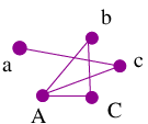
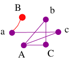
There will be a vertex in and for each of the directions . The vertex in corresponding to is red and all others are purple. There are purple edges in for each edge in . And has a single red edge for the turn (the turn represented by an edge in , but not in . is obtained from by adding black edges connecting the pairs of vertices , , and (these black edges correspond precisely to the edges and of ).
, , and respectively look like (in these figures, A will be used to denote , B will be used to denote , and will be used to denote ):

We now relate the definitions of ideal Whitehead graphs, etc, given above to those only relying on the attracting lamination for a fully irreducible outer automorphism. The purpose will be to show that an ideal Whitehead graph is indeed an outer automorphism invariant. Each of the following definitions can be found in [HM11].
Definition 2.12.
A fixed point is repelling for the action of if it is an attracting fixed point for the action of , i.e. if there exists a neighborhood of such that, for each neighborhood of , there exists an such that for all and .
Let be a train track representative of a nongeometric, fully irreducible, rotationless and let be a principal lift of , i.e. a lift to the universal cover such that the boundary extension has at least three nonrepelling fixed points. We denote the boundary extension of by . will denote the lift of the attracting lamination to the universal cover of . The ideal Whitehead graph, , for is defined to be the graph where:
(1) The vertices correspond to nonrepelling fixed points of .
(2) The edges connect vertices corresponding to and precisely when and are the ideal (boundary) endpoints of some leaf in .
We then define the ideal Whitehead graph for by , leaving out components having two or fewer vertices.
Since the attracting lamination is an outer automorphism invariant (and, in particular, the properties of leaves having nonrepelling fixed point endpoints and sharing an endpoint are invariant), the definition we just gave does not rely on the choice of representative for a given . Thus, once we establish equivalence between this definition and that given at the beginning of this subsection, it should be clear that the ideal Whitehead graph is an outer automorphism invariant.
Corollary 2.13 below is Corollary 3.2 of [HM11]. It relates the definition of an ideal Whitehead graph that we gave above Example 2.11 to that given in Definition 2.12.
For Corollary 2.13 to actually make sense, one needs the following definitions and identification from [HM11]. A cut vertex of a graph is a vertex separating a component of the graph into two components. denotes the lift of to the universal cover of (having countably many disjoint copies of , one for each lift of ).
Let be an irreducible train track representative of an iterate of such that:
(1) each periodic vertex is fixed and
(2) each periodic direction at such a is fixed.
Choose one of these fixed vertices . Suppose is a lift of to the universal cover, is a lift of fixing , and is a direction at fixed by . Furthermore, let be the edge at whose initial direction is . The ray determined by (or by ) is defined as . This is a ray in converging to a nonrepelling fixed point for . Such a ray is called singular if the vertex it originates at is principal (i.e. is principal). With these definitions:
(1) the vertices of correspond to singular rays based at and
(2) directions and represent endpoints of an edge in if and only if is a singular leaf of realized in , where and are the rays determined by and respectively.
Noticing that the ideal (boundary) endpoints of singular rays are precisely the nonrepelling fixed points at infinity for the action of , combining this with what has already been said, as well as Corollary 2.13 and what follows, we have the correspondence proving ideal Whitehead graph invariance.
Corollary 2.13.
[HM11]
Let be a principal lift of . Then:
(1) is connected.
(2) .
(3) For , and intersect in at most one vertex. If they do intersect at a vertex , then is a cut point of , in fact separates and in .
By [Lemma 3.1, HM11], in our case (where there are no PNPs), there is in fact only one and so the above corollary gives that .
This concludes our justification of how an ideal Whitehead graph is an outer automorphism invariant. Consult [HM11] for clarification of the relationship between ideal Whitehead graphs and R-trees or for other ideal Whitehead graph characterizations.
2.9 Folds, Decompositions, and Generators
John Stallings introduced “folds” in [St83]. Bestvina and Handel use in [BH92] several versions of folds in their construction of TT representatives of irreducible . We use folds in Section 3 for defining and proving ideal decomposition existence.
Let be a homotopy equivalence of marked graphs. Suppose that as edge paths, where the edges emanate from a common vertex . One can obtain a graph by identifying and in such a way that projects to under the quotient map induced by the identification of and . is also a homotopy equivalence and one says that and are obtained from by an elementary fold of and . [St83, BH92]
One can generalize this definition by only requiring that and be maximal, initial, nontrivial subsegments of edges emanating from a common vertex such that as edge paths and such that the terminal endpoints of and are in . Possibly redefining to have vertices at the endpoints of and , one can fold and as and were folded above. If both and are proper subedges then we say that is obtained by a partial fold of and . If only one of and is a proper subedge (and the other is a full edge), then we call the fold a proper full fold of and . In the remaining case where and are both full edges, we call the fold an improper full fold. [St83, BH92]
Now let be a free basis for the free group . From [N86] we know that any can be written as a composition of “Nielsen generators” having one of the following two forms (Nielsen gave a longer list, but these suffice):
- (1)
for some (and for all with )
- (2)
a permutation of preserving inverses (if , then ).
Definition 2.14.
In general, we will call an automorphism such as in (1) the Nielsen generator (or just generator) .
Consider two metric roses and with respective edge-labelings and
and markings where the homotopy class of each in and each in are identified with the free basis element under the respective markings. Consider a homotopy equivalence that linearly maps over and, for each , linearly maps over . Let where is mapped by over and is mapped by over . Now consider a quotient map (a “proper full fold”) identifying with . There exists a homeomorphism such that , i.e. and give the same induced map of fundamental groups. In fact, the homeomorphism linearly maps over and linearly maps each other over . Sometimes we instead call the proper full fold.
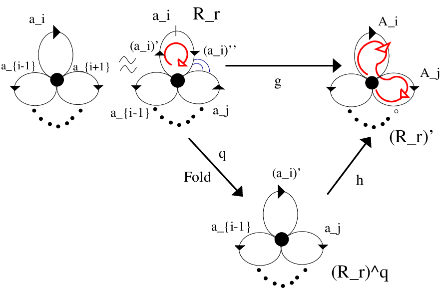
Under the identification, for each , of the homotopy classes of the and with the free basis element , the induced automorphism is the automorphism where and for all . We say that in the pervious paragraph corresponds to the Nielsen generator . We have similar situations for cases where maps linearly over and , or is replaced by its inverse, or both and are replaced by their inverses.
Stallings showed in [St83] that one can decompose a tight (in the sense defined in Subsection 2.3 above) homotopy equivalence of graphs as a composition of elementary folds together with a final homeomorphism. In the circumstance where the elementary folds are proper full folds of roses, the elements of this decomposition have induced Nielsen generators, as described above.
Ideally, the Nielsen generators in a decomposition of would all be of form (1) above and there would be a representative of where
- •
is a marked rose,
- •
( corresponds to ),
- •
the Stallings fold decomposition corresponds to the Nielsen generator decomposition in the sense that (where is the marking on ) for each , and
- •
each is a proper full fold of a rose.
In Section 3 we prove that such is the case in the scenario we want it for.
3 Ideal Decompositions
As mentioned in Subsection 2.9, TT representatives are composed of elementary folds, followed by a homeomorphism. The ideal situation would be to have a TT representative for each composed only of proper full folds of roses and a homeomorphism inducing a trivial permutation. We would further like for the automorphism corresponding to to have several properties.
In this section we show that for an ageometric, fully irreducible such that is Type (*) pIW we have a representative of a rotationless power decomposed as desired.
For Proposition 3.3, we need the following from [HM11]: Let an ageometric, fully irreducible be such that is a Type (*) pIWG , then is rotationless if and only if the vertices of are fixed by the action of .
We will also need the following lemmas:
Lemma 3.1.
Let be a PNP-free TT representative of a fully irreducible and let be a decomposition of into homotopy equivalence of marked metric graphs. Let denote the composition . Then is also a PNP-free TT representative of (and, in particular, ).
Proof: Suppose that had a PNP and let be such that the path is fixed (up to homotopy rel endpoints), i.e. rel endpoints. Let . First notice that cannot be trivial or would be trivial, contradicting that is a PNP.
. Now, rel endpoints and so rel endpoints (just compose the homotopy with ) But that means that is homotopic to relative endpoints. Making a PNP for contradicting that is PNP-free. Thus, must be PNP-free, as desired.
Let be the marking on . Since is a homotopy equivalence, gives a marking on and and just differ by a change of marking. Thus, and are representatives of the same outer automorphism .
QED.
Lemma 3.2.
Let be a PNP-free train track representative of a fully irreducible such that has fixed directions. Let
be the Stallings fold decomposition for . Let be such that . Let be the fixed directions for and let for each and . Then cannot identify any of the directions .
Proof: Let be the fixed directions for and let for each and . Suppose that identified any of the directions , then we would have that had fewer than directions in its image, contradicting that it has fixed directions.
QED.
Proposition 3.3.
Let an ageometric, fully irreducible be such that is a Type (*) pIW graph. Then there exists a PNP-free, rotationless representative of a power of on the rose. Further, the representative can be decomposed as a sequence of proper full folds of roses.
Proof: Suppose is as described in the proposition. Since is ageometric, there exists a PNP-free TT representative of a power of . Let be such that fixes all of ’s periodic directions ( is rotationless). Then is also a PNP-free TT representative of some . Since has no PNPs (meaning ), since fixes all of its periodic directions (in particular for all ), and since the ideal Whitehead graph of (hence ) is a Type (*) pIW graph, must have a vertex with fixed directions. Thus, must be one of the only three graphs of rank with a valence or higher vertex:

If , then will be the desired representative. We will show that, in this case we have the desired decomposition. However, first we will show that cannot be or by ruling out all possibilities for folds in the Stallings fold decomposition for in the cases of and .
If we had , then the vertex with fixed directions could only be . must have an illegal turn unless it were a homeomorphism, which it could not be and still be irreducible. Notice that could not be mapped to in a way not forcing an illegal turn at , as this would mean that either we would have an illegal turn at (if were wrapped around some ) or we would have backtracking on (contradicting that is a TT map, so must be locally injective on edge interiors). Because all of the directions at are fixed by , if had an illegal turn, it would have to occur at (as no two of the fixed directions can share a gate).
The turns at are , , and . However, we only need to rule out illegal turns at and , as the situations with and are identical.
First, suppose that the illegal turn at were , so that the first fold in the Stallings decomposition would have to be of . Fold maximally to obtain . The fold cannot completely collapse , as this would change the homotopy type of . Also, we can assume the fold is maximal or the next fold in the sequence would just anyway be a continuation of the same fold.

Let be the induced map as in [BH92] and explained in Subsection 2.9 above. Since the fold of was maximal, must be legal. Since was a TT map, and thus was locally injective on edges of (on the edge in particular), and must also be legal. But then would fix all directions at both vertices of (since it still must fix all directions at ). This would make a homeomorphism, again contradicting irreducibility. Thus, could not have been the illegal turn at . This leaves us to rule out .
Suppose that the illegal turn at were , so that the first fold in the Stallings decomposition would have to be of . Fold maximally (we can again assume the fold is maximal). Let be the induced map of [BH92] and Subsection 2.9. Either
I. all of is folded with all of or a power of ;
II. all of is folded with part of or a power of ;
III. part of is folded with all of or a power of ; or
IV. part of is folded with part of or a power of .
If (I) or (II) held, would be a rose and would give a representative on the rose, returning us to the case of . So we just need to analyze (III) and (IV).
Consider first (III), i.e. suppose part of is folded with part of or a power of :

Let be such that with being the single fold performed thus far. could not identify any of the directions at : could not identify and or would have had back-tracking on ; could not identify and or would have had back-tracking on ; and could not identify and because the fold was maximal. But then all the directions of would be fixed by , making a homeomorphism and the decomposition complete. However, this would make consist of the single fold and a homeomorphism, contradicting that ’s irreducibility. So, in analyzing what might happen if were the illegal turn for at , we are left to analyze (IV):

Suppose part of were folded with all of (or a power of ). Again let be such that , where is the single fold performed thus far. If did not identify any of the directions at , it would be a homeomorphism, causing the same contradiction with ’s irreducibility as above. But could not identify any of the directions at : could not identify and for the same reasons as above; could not identify and , as the fold of and was maximal; and cannot identify and of would have had backtracking on . We have thus shown that all cases where are either impossible or yield the desired representative on the rose.
We are left to analyze when . In this case, must be the vertex with fixed directions. As with , because must fix all directions at , if had an illegal turn (which it still has to) the turn would be at . Without loss of generality assume the illegal turn is . Maximally fold . If all of and were folded, this would change the homotopy type. Thus also assume (again without losing generality) that either 1. all of is folded with part of or 2. only proper initial segments of and are folded with each other. If (1) holds, we get a PNP-free TT representative on the rose. So suppose (2) holds. Let be the induced map of [BH92]. The fold and look like:

The new vertex has 3 distinct gates ( is legal since the fold was maximal and and must also be legal or would have had back-tracking on or , respectively). This leaves the situation where the entire decomposition is a single fold with a homeomorphism, again leading to the contradiction of being reducible.
Having ruled out all cases, we have completed the analysis of and thus proved that we have a PNP-free representative of a power of on the rose.
Let be the PNP-free train track representative of on the rose. Let
be the Stallings decomposition for . Each is either an elementary fold or locally injective (in which case it would be a homeomorphism). We can assume that is the only homeomorphism. Let . Since has precisely gates, has precisely one illegal turn. We first determine what could be. cannot be a homeomorphism or we would have , making reducible. Thus, ’s vertex contains an illegal turn for . We maximally fold the illegal turn. Suppose first that the fold is a proper full fold. (If the fold is not a proper full fold, then see the analysis below about what would happen with an improper or partial fold.)

By Lemma 3.2, cannot have more than one turn such that is degenerate (we will call such a turn an order one illegal turn for ). If it has no order one illegal turn, then must be a homeomorphism and we have determined the entire decomposition. So suppose that has an order one illegal turn and maximally fold this illegal turn. Continue as such until either is obtained, in which case the desired decomposition has been found, or until the next fold is not a proper full fold.
The next fold cannot be an improper full fold because this would change the homotopy type of the rose. So suppose, without loss of generality, that this first fold other than a proper full fold is a partial fold of and .

As in the analysis of the case of above, the next fold has to be at or the next generator would be a homeomorphism, which does not make sense since is not a rose and the image of is a rose. Since the previous fold was maximal, the illegal turn cannot be . The illegal turn also cannot be or , since this would imply had backtracking on edges, contradicting that is a train track. Thus, was not possible in the first place, meaning that all of the folds in the Stallings decomposition must be proper full folds between roses.
Since all folds in the Stallings decomposition are proper full folds of roses, it is possible to index the edge sets as
so that
(a) where , , and
(b) for all .
Suppose we similarly index the directions .
Let be the homeomorphism in the Stalling’s decomposition and suppose that gave a nontrivial permutation of the second indices of the directions. Some power of the permutation would be trivial. Replace by . We rewrite the decomposition of as follows. Let denote the permutation of second indices defined by . Then, for define by where and . Adjust the corresponding proper full folds accordingly. This decomposition still gives , but now the permutation caused by the final homeomorphism is trivial.
This concludes the proof that the PNP-free TT representative of a power of on the rose can be decomposed as a sequence of proper full folds between roses and thus the proof of the proposition.
QED
Representatives such as that given in Proposition 3.3 will be called ideally decomposable and the decomposition an ideal decomposition. We establish here notation used for discussing ideally decomposed representatives and restate the results in that notation. That (4) and (3a) hold (i.e that is not a homeomorphism permuting the direction second indices) can be ascertained from the Proposition 3.3 proof.
Ideal Decomposition Standard Statement and Notation:
Let be an ageometric, fully irreducible outer automorphism such that has vertices. Then Proposition 3.3 gives a PNP-free representative of a rotationless power of with a decomposition
, where:
(1) the index set is viewed as the set / with its natural cyclic ordering;
(2) each is a rose;
(3) we can index the sets as
and as
( and for each ) so that
(a) where , , and and
(b) for all
(we denote by , by , by , and by ); and
(4) for all such that , we have , where . ( fixes every direction except for ).
Additionally,
- •
will denote the set of directions corresponding to .
- •
.
- •
if and if .
- •
will denote , which will sometimes be called the unachieved direction for because it is not in the image of (the “” in is for “unachieved”).
- •
will denote and sometimes be called the twice-achieved direction for , as it is the image of both () and () under (the “” in is for “(twice) achieved” and the “” in and is for “pre”).
- •
will denote
- •
will denote the subgraph of containing
- (1)
all black edges and vertices (given the same colors and labels as in ) and
- (2)
all colored edges representing turns in taken by .
- (1)
- •
If we additionally require that is ageometric and fully irreducible and that is a Type (*) pIW graph, then we will say is of Type (*). (By saying is of Type (*), it will be implicit that, not only is ageometric and fully irreducible, but is ideally decomposed, or at least ideally decomposable).
Remark 3.4.
We refer to as for all in circumstances where we believe it will not cause confusion. In these circumstances we may also refer to as .
While we may abuse notation by writing instead of , unless otherwise specified, will always denote an element of (or when specified), where the index of will not necessarily match the index of the corresponding element of (or ). will still denote .
Additionally, for reasons of typographical clarity we sometimes put parantheses around the subscripts.
4 Lamination Train Track (LTT) Structures
This section contains our definitions for several different abstract and specific notions of “lamination train track (LTT) structures.” M. Bestvina, M. Feighn, and M. Handel discussed in their papers slightly different notions of train track structures than the notions we describe here. However, those we describe in this section contain as smooth paths realizations of leaves of the attracting lamination for the outer automorphism. This fact makes them useful for ruling out the achievability of particular ideal Whitehead graphs and for constructing the particular representatives we seek. The need for all of the properties included in the LTT definitions should become clear in Section 5 when we prove the necessity of the “Admissible Map Properties.”
4.1 Abstract Lamination Train Track Structures
Definition 4.1.
A smooth train track graph is a finite graph satisfying:
- STTG1:
-
has no valence-1 vertices;
- STTG2:
-
each edge of has 2 distinct vertices (single edges are never loops); and
- STTG3:
-
the set of edges of can be partitioned into two subsets, (the “black” edges) and (the “colored” edges), such that each vertex is incident to at least one and at least one .
Two train track graphs will be considered equivalent if they are isomorphic as graphs.
Definition 4.2.
A path in a smooth train track graph is smooth if no two consecutive edges of the path are in and no two consecutive edges of the path are in .
We now give our first abstract notion of a lamination train track (LTT) structure.
Definition 4.3.
A Lamination Train Track (LTT) Structure is a smooth colored train track graph (black edges will be included but not considered colored) satisfying each of the following:
- LTT1:
-
Vertices are either purple or red.
- LTT2:
-
There are an even number of vertices and they are labeled via a one-to-one correspondence with a set . (In the case of an LTT structure for a Type (*) representative , the and will be the initial and terminal directions of the edges of ).
- LTT3:
-
No pair of vertices is connected by two distinct colored edges.
- LTT4:
-
Edges of are of the following 3 types:
- (Black Edges):
-
A single black edge connects each pair of vertices of the form . There are no other black edges. In particular, there is precisely one black edge containing each vertex.
- (Red Edges):
-
A colored edge is red if and only if at least one of its endpoint vertices is red.
- (Purple Edges):
-
A colored edge is purple if and only if both endpoint vertices are purple.
- LTT5:
-
The partition of the set of edges of , where is the set of black edges of and is the set of colored edges of , satisfies (STTG3).
is an augmented LTT structure with legal structure if it is obtained from by adding some green edges to the colored edges of and the green edges satisfy:
- LTT6:
-
At least one vertex of each green edge is red.
- LTT7:
-
A green edge and a nongreen edge never connect the same vertex pair.
Definition 4.4.
Two LTT structures differing by an ornamentation-preserving (label and color preserving), vertex-preserving homeomorphism will be considered equivalent.
Standard LTT Structure Notation and Terminology: In the context of an LTT Structure :
- •
An edge connecting a vertex pair will be denoted [].
- •
The interior of [] will be denoted ().
(While the notation [] may be ambiguous when there is more than one edge connecting the vertex pair , we will be clear in such cases as to which edge we refer to.) - •
will denote []
- •
Red vertices will be called nonperiodic (direction) vertices.
- •
Red edges will be called nonperiodic (turn) edges.
- •
Purple vertices will be called periodic (direction) vertices.
- •
Purple edges will be called periodic (turn) edges.
- •
The purple subgraph of an LTT structure will be called the potential ideal Whitehead graph associated to and will be denoted . For a finite graph , we will say that is an LTT Structure for .
- •
will denote the colored subgraph of the LTT structure and will be called the colored subgraph associated to (or of) .
- •
We say that the LTT structure is admissible if is additionally birecurrent as a graph, i.e. if there exists a smooth line in such that each edge of occurs infinitely often in each end of the line.
- •
For an augmented LTT structure with legal structure , we denote the set of green edges of by and call elements of green illegal turn edges (or say that they correspond to illegal turns).
4.1.1 Type (*) LTT Structures for Type (*) pIWGs
The following specialized abstract LTT structure is tailored for the case of a fully irreducible, ageometric such that is a Type (*) pIWG. For this definition, a (potential) ideal Whitehead graph must be designated, but the structure does not use or record any other information about .
Definition 4.5.
A Type (*) Lamination Train Track Structure is an LTT structure a Type (*) pIW graph for such that:
- LTT(*)1:
-
has only a single red vertex (all other vertices are purple).
- LTT(*)2:
-
has a unique red edge.
- LTT(*)3:
-
.
Standard Type (*) Notation and Terminology: In the context of a Type (*) LTT structure for :
- •
The label on the unique red vertex will sometimes be written and called the unachieved direction.
- •
The unique red edge is denoted , or [], and the label on its purple vertex is denoted .
- •
is contained in a unique black edge, which we call the twice-achieved edge.
- •
The other twice-achieved edge vertex will be labeled by and called the twice-achieved direction.
- •
For a Type (*) LTT structure to be admissible, we will require that it is admissible as an LTT structure and, in particular:
- LTT(*)4:
-
has no valence-1 vertices contained in purple or red edges of the form [].
4.1.2 Based Lamination Train Track Structures
Instead of relying on information about for , the following LTT structure focuses on the graph for a representative of .
Definition 4.6.
Let be a connected marked graph with no valence-one vertices. An LTT Structure with Base Graph is an LTT structure such that:
- LTT(Based)1:
-
For each vertex and direction , there exists a vertex in labeled by . In particular, the vertices of are in one-to-one correspondence with
- LTT(Based)2:
-
Edges of are of the following 3 types:
- (Purple Edges)
-
connect the purple vertices in corresponding to certain distinct pairs of directions at a common vertex of (we will call such pairs of directions periodic turns);
- (Red Edges)
-
connect the vertices in corresponding to certain distinct pairs of directions at a common vertex of such that at least one direction in the pair is represented by a red vertex in . (We will call such pairs of directions nonperiodic turns);
- (Black Edges)
-
connect precisely vertex pairs where .
Based LTT Structure Terminology: In the context of Definition 4.6, for a given vertex :
- •
We call the union of the purple edges , where , the stable Whitehead graph at .
- •
We call the union of the purple and red edges [] corresponding to turns , where , the local Whitehead graph at .
Definition 4.7.
Let be an r-petaled rose with vertex . A Type (*) LTT Structure with base graph is an LTT structure with base graph additionally satisfying:
- LTT(*)(Based)1:
-
is a Type (*) pIW graph (and is actually PI()).
An Augmented Type (*) Lamination Train Track Structure for with Base Graph is an augmented LTT structure with legal structure additionally satisfying:
- LTT(*)(Based)2:
-
is a Type (*) LTT structure with base graph .
- LTT(*)(Based)3:
-
contains only a single edge, which we denote , or just , and call the of or edge corresponding to the illegal turn;
We describe here what it means for two based LTT structures to be equivalent.
Definition 4.8.
Suppose and are LTT structures with respective base graphs and . A homeomorphism extends to an ornamentation-preserving homeomorphism if, for each edge there exists a homeomorphism and for each edge there exists a homeomorphism such that the following commutes:
One would also say in such a circumstance that restricts to .
LTT structures and with respective bases and are equivalent if there exists an ornamentation-preserving homeomorphism of based LTT structures restricting to a label-preserving homeomorphism of marked graphs.
4.1.3 Maps of Based Lamination Train Track Structures
Let and be LTT structures with respective base graphs and . Let be a homotopy equivalence. Recall that induces a map of turns . additionally induces a map on the corresponding edges of and (if the appropriate edges exist in ):
Definition 4.9.
Let and be LTT structures with respective base graphs and . We say is a map of colored subgraphs induced by if:
- 1.
sends the vertex labeled in to that labeled by in ;
- 2.
sends the edge [] in to the edge [] in ;
- 3.
maps each into ;
- 4.
maps each isomorphically onto
We now describe what it means for a continuous map of marked graphs to extend to a map of based LTT structures.
Definition 4.10.
Suppose that and are LTT structures with respective base graphs and . Let be a homotopy equivalence such that . A map induced by is an extension of taking the interior of the black edge of corresponding to the edge to the interior of the smooth path in corresponding to . In this case we say that is the extension of to the continuous map of based LTT structures and that extends to .
Definition 4.11.
A vertex-preserving homeomorphism extends to an ornamentation-preserving homeomorphism if there exist homeomorphisms and homeomorphisms such that the following diagram commutes:
One would also say in this circumstance that restricts to .
We now describe what it means for two based LTT structures to be equivalent.
Definition 4.12.
Suppose that and are LTT structures with respective base graphs and . If there exists a vertex-preserving homeomorphism extending to an ornamentation-preserving homeomorphism then we say that induces an equivalence of and and that and are equivalent based LTT structures.
4.1.4 Generating Triples
Since we deal with representatives decomposed into Nielsen generators, we will use an abstract notion of a “generating triple.”
Definition 4.13.
A generating triple is a triple such that
- (1)
is a Nielsen generator of marked graphs defined by for some , , and ;
- (2)
is an LTT structure with base graph ;
- (3)
is an LTT structure with base graph ;
- (4)
is the induced map of based LTT structures;
- (5)
contains the red edge where and ; and
- (6)
either or is a red vertex in .
The following establishes equivalences for generating triples of based LTT structures.
Definition 4.14.
Suppose that and are generating triples. Let be the map of LTT structures induced by and let be the map of LTT structures induced by .
We say that and are equivalent generating triples if there exist homeomorphisms and such that
- •
induces an equivalence of and as based LTT structures,
- •
induces an equivalence of and as based LTT structures,
- •
and the following diagram commutes:
4.2 LTT Structures of Type (*) Representatives
We now give a few definitions that will enable us to apply the abstract definitions given earlier to the setting of Type (*) representatives, as defined in Section 3.
Definition 4.15.
Let be ideally decomposable (with the condition on directions being fixed dropped), let be the set of edges of with a particular orientation, and let . For an oriented edge , we let and (the terminal direction of ).
The Colored local Whitehead graph at the vertex , , is the uncolored graph but with the subgraph colored purple and colored red (including the nonperiodic vertices).
Let be the graph obtained from by removing a contractible neighborhood, , of the vertex of and adding vertices and at the corresponding boundary points of each partial edge , for each . A Lamination Train Track Structure for is formed from by identifying the vertex labeled in with the vertex labeled in . The vertices for nonperiodic directions are red, the edges of remain black, and all periodic vertices remain purple.
An LTT structure is given a smooth structure via a partition of the edges at each vertex into the two sets: (containing all black edges of ) and (containing all colored edges of ). A smooth path will be a path alternating between colored and black edges.
The Augmented Lamination Train Track Structure for , , is formed from by adding a green edge for each illegal turn of .
Remark 4.16.
We record here the following remarks about LTT structures:
- (1)
could also be built from by adding a black edge connecting each vertex pair .
- (2)
Each edge image path determines a smooth path in that transverses the black edge , then the colored edge , then the black edge , and so on, until it ends with the black edge . This observation is related to one of the most important properties of LTT structures for fully irreducible representatives, i.e. they contain leaves of the attracting lamination as locally smoothly embedded lines.
- (3)
The train track structures we define are not quite the same as those in [BH97].
Definition 4.17.
Let be an ideally decomposed Type (*) representative of with the standard ideal decomposition notation. Then will denote the LTT structure and will denote the subgraph of containing
(1) all black edges and vertices (given the same colors and labels as in ) and
(2) all colored edges representing turns in for some .
For any , we have a direction map and an induced map of turns . The induced map of LTT Structures is such that
(1) the vertex corresponding to a direction is mapped to the vertex corresponding to the direction ,
(2) the colored edge [] is mapped linearly as an extension of the vertex map to the edge [] [], and
(3) the interior of the black edge of corresponding to the edge to the interior of the smooth path in corresponding to .
Remark 4.18.
It still makes sense to define when is only irreducible (not fully irreducible) and possibly even is not ageometric. The difference will be that, while the purple subgraph will be , it will not necessarily be . If had more than one vertex, one would define by creating a colored graph for each vertex, removing an open neighborhood of each vertex when forming , and then continuing with the identifications as above in . Dropping the condition on having fixed directions more drastically changes what definitions actually make sense or what they look like if they do make sense.
5 Admissible Map Properties
The aim of this section is establishing additional properties held by any Type (*) representative. In particular, we determine several necessary characteristics of LTT structures arising in an ideal decomposition of a Type (*) representative and give the background to identify (as described in Section 7) the only two possible types of (fold/peel) relationships between any LTT structures and in an ideal decomposition. The properties proved necessary in this section will be called “Admissible Map Properties.” They are summarized in the final subsection, Subsection 5.10.
In subsequent sections, we will define and outline a method for associating, a diagram (the “AM Diagram”) to a Type (*) pIW graph . This diagram will contain a loop for each map having the Admissible Map Properties we establish in this section. Thus, in particular, the diagram contains a loop for any Type (*) representative with . If no loop in the diagram gives an irreducible, PNP-free representative with , then we know that does not occur as for any ageometric, fully irreducible . We will use this fact to rule out the possibility of achieving certain graphs in Sections 13 and 14. We also give in subsequent sections methods for constructing the Type (*) representatives, if they do exist.
The conditions of an ideal decomposition will be relaxed slightly for many of the subsections of this section in order to highlight the necessity of certain properties (we will make it clear when representatives will also be required to be ideally decomposed of Type (*)). For each of these subsections, will be an irreducible TT representative of semi-ideally decomposed as: , where the decomposition differs from an ideal decomposition (as described in the end of Section 3) in that the periodic directions may not be fixed. The notation for the decomposition will also be as in the end of Section 3 and saying that is of Type (*) will still mean that is a Type (*) pIWG. We will use the standard ideal decomposition notation, even when our decomposition in only semi-ideal.
We begin this section by proving a preliminary lemma that will be used later in this section to prove the necessity of the “Admissible Map Properties.”
5.1 Cancellation and a Preliminary Lemma
Before stating the lemma, we clarify for the reader what is meant by “cancellation”.
Definition 5.1.
We say that an edge path in has cancellation if for some . We say that has no cancellation on edges if for no and edge does the edge path have cancellation.
We are now ready to state and prove the lemma.
Lemma 5.2.
Suppose that is a semi-ideally decomposed TT representative of with the standard ideal decomposition notation. For this lemma we index the generators in the decomposition of all powers of so that (, but we want to use the indices to keep track of a generator’s place in the decomposition of ). With this notation, will mean . Then:
(1) for each ), no has cancellation;
(2) for each and each edge , the edge is contained in the edge path ; and
(3) if , then the turn is in the edge path , for all .
Proof: Let be minimal so that some has cancellation. Before continuing with our proof of (1), we first proceed by induction on to show that (2) holds for . For the base case observe that for all . Thus, if and then is precisely the path and so we are only left for the base case to consider when . If , then and so the edge path contains , as desired. If , then and so the edge path also contains in this case. Having considered all possibilities, the base case is proved.
For the inductive step, we assume that contains and show that is in the edge path . Let for some edges . As in the base case, for all , is precisely the edge path . Thus (since is an automorphism and since there is no cancellation in for ), where each and where no , , or is an illegal turn. So each is in , as desired. We are only left to consider for the inductive step the cases where and where .
If , then , and so (where no , , or is an illegal turn), which contains , as desired. If instead , then and so , which also contains . Having considered all possibilities, the inductive step is now also proven and the proof is complete for (2) in the case of .
We now finish our proof of (1). We are still assuming that is minimal so that has cancellation for some . Let be such that has cancellation. Let , for , be edges in so that . Since was minimal, either has cancellation for some or for some . Since each is a generator, no has cancellation. Thus, there exists an such that . Since we have already proved (1) for all , we know that the edge path contains . Then contains cancellation, which implies that for some (with ) contains cancellation, which contradicts that is a train track map.
We now prove (3). Let By (2) we know that the edge path contains . Let be such that . Then where for all . Thus contains , as desired.
QED.
5.2 LTT Structures, Birecurrency, and AM Property I
LTT structures were defined in Section 4 and the “birecurrency”(defined below) of each LTT structure in a semi-ideal decomposition is the first property we will prove necessary for a Type (*) representative, i.e. AM Property I.
Definition 5.3.
We will say that a smooth train track graph is birecurrent if there exists a locally smoothly embedded line in that crosses each edge of infinitely many times as and as .
Proposition 5.4.
Let be a Type (*) representative of . Then is birecurrent.
Our proof of this proposition will require the following lemmas recording the relationship between the local Whitehead graph for , , and the realization of the leaves of the attracting lamination, , for . The proofs will use facts about laminations that can be found in [BFH97] and [HM11], but will not be recorded here.
Lemma 5.5.
Let be a Type (*) representative of . The only turns possible in the realization in of a leaf of the attracting lamination for are those corresponding to edges in . Conversely, each turn represented by an edge of is a turn of some (hence all) leaves of (as realized in ).
Proof: To prove the forward direction, we first notice, as follows, that each edge has a fixed point in its interior. Since is irreducible, some contains a path with at least three edges (some contains at least two edges of , including and then contains at least three edges). Let , with each . Again, since is irreducible, for some , the edge path contains either or . Thus, contains either or in its interior, implying that has a fixed point in its interior. This then tells us that, for each edge , there is a periodic leaf of obtained by iterating a neighborhood of a fixed point of .
Consider any turn taken by the realization in of a leaf of . Since periodic leaves are dense in the lamination, either or (where or ) is a subpath of any periodic leaf of the lamination. In particular, either or is a subpath of the leaf obtained by iterating a neighborhood of a fixed point of for any , so is contained in some , for each . Thus, is represented by an edge in , as desired. This concludes the forward direction.
We now prove the converse. The presence of the turn as an edge of indicates that, for some and , is a subpath of . We showed above that each has a fixed point in its interior and hence that there is a periodic leaf of obtained by iterating a neighborhood of the fixed point of . is a subpath of this periodic leaf and (since periodic leaves are dense) of every leaf of . Since the leaves contain as a subpath, they contain as a subpath, and thus the turn . This concludes the proof of the converse, and hence lemma.
QED.
We will need one more definition for the proof of the second lemma.
Definition 5.6.
Let be a train track representative of a fully irreducible, ageometric . Let be a smooth (possibly infinite) path in . The path (or line) in corresponding to is , where
,
where each , each is the black edge of corresponding to the edge , and each is a colored edge.
Lemma 5.7.
Let be a TT representative of a fully irreducible, ageometric . Then contains smooth paths corresponding to the realizations in of the leaves of .
Proof of Lemma: Consider the realization of a leaf of and any single subpath in . If it exists, the representation in of would be by the path
, as above. Lemma 5.5 above tells us that and are edges of and hence are colored edges in . The path representing in thus exists and alternates between colored and black edges. By looking at overlapping subpaths, we can see that the path in corresponding to has no consecutive colored or black edges and so is smooth. We have proved the lemma.
QED.
We are now ready for the proof of the proposition.
Proof of Proposition 5.4: We need that contains a locally smoothly embedded line crossing over each edge of infinitely many times as and as . We will show that the path corresponding to the realization of a leaf of is such a line. We first consider any colored edge [] in . By Lemma 5.5, must contain either or as a subpath. Birecurrency of the lamination leaves of a fully irreducible implies that must cross the subpath or infinitely many times as and as . We showed in Lemma 5.7 above that this means that contains either or infinitely many times as and as . This concludes the proof for a colored edge.
Now consider a black edge . Each vertex is shared with a colored edge. Let [] be such an edge. As shown above, or occur in realizations infinitely many times as and as . In particular, it crosses over infinitely many times as and as . And so crosses over infinitely many times as and as . This concludes the proof.
QED.
In combination with Proposition 5.4, the second of the following two lemmas proves the necessity of AM Property I. The first (Lemma 5.8) is used in the proof of the second (Lemma 5.10) .
Lemma 5.8.
Let be a semi-ideally decomposed train track representative. Each has the same number of gates (and thus periodic directions).
Proof: Suppose, for the sake of contradiction, that had more gates than . Let be such that maps each gate of to a single direction and let be such that maps each gate of to a single direction. Let be the set of gates for , let be the periodic direction of for each , let be the set of gates for , and let be the periodic direction of for each . Consider . Let . Then is mapped by into and, consequently, . This implies that , which has at most elements. But this contradicts having more gates that . Thus, all have the same number of gates.
QED.
Remark 5.9.
If is an ideally decomposed Type (*) representative, then the above lemma shows that each has the same number of purple periodic vertices.
Lemma 5.10.
If is an ideally decomposed Type (*) representative of with the standard ideal decomposition notation, then each is also an ideally decomposed Type (*) representative of for some .
Proof of Lemma: If is an ideal decomposition of , then can be decomposed as
What we need to show is that this decomposition of is an ideal decomposition and that is a representative of for some (since we already know that is ageometric and fully irreducible, as well as that is a Type (*) pIW graph, we know that all of these things must also be true of any ). Properties (1)-(3) of an ideal decomposition hold for the decomposition of because they hold for the decomposition of and the decompositions have the same and (just renumbered). By the previous lemma we know that also has gates. Thus, some fixes directions. Since is not in the image of , it cannot be in the image of . We thus also know that (4) holds for the decomposition of and we are only left to prove that is a representative of . Now, is a representative of and . Let be the marking on . Since is a homotopy equivalence, gives a marking on and and just differ by a change of marking. Thus, and are representatives of the same outer automorphism, i.e. . This concludes the proof.
QED.
Remark 5.11.
The same proof works to prove the statement where “ideally” is replaced by “semi-ideally.”
We have thus shown that every ideally decomposed Type (*) representative satisfies
- AM Property I:
-
Each LTT structure is birecurrent.
5.3 Periodic Directions and AM Property II
The main goal of this subsection is Proposition 5.14, giving AM Property II for a Type (*) representative of such that .
We add to the notation already established that and .
The following lemma is used in the proof of Proposition 5.14.
Lemma 5.12.
is an illegal turn for .
Proof: Recall that .
Since ,
,
which is degenerate. So is an illegal turn for , as desired.
QED.
Definition 5.13.
As a result of the previous lemma, for the generator , we will sometimes call the green illegal turn in (even though does not technically live in , but in the augmented LTT structure for ).
We are now ready to prove the proposition.
Proposition 5.14.
Let be semi-ideally decomposed (though not necessarily irreducible). has periodic directions if and only if, for each , the illegal turn contains , ie, either or . In fact, if each contains , the image of contains all directions in except .
Proof: We start by proving the forward direction. Suppose that our map has periodic directions and, for the sake of contradiction, that the illegal turn does not contain . Let and . Then and , which means that
and so and share a gate. But is already in a gate with more than one element and we already established that and . So has a maximum of gates. Since each has the same number of gates, this would imply that has a maximum of gates, giving a contradiction. The forward direction is thus proved.
Now suppose that, for each , the illegal turn for the generator always contained the unachieved direction for the generator . We will proceed by induction to prove that would then have distinct gates. In fact, we will show that the image of is missing precisely , where .
For the base case we need that has distinct gates. By our assumptions, . The direction map for , , is defined by and for all with . Thus, the image of includes distinct directions and is missing precisely . Also, the only direction with two preimages is . This concludes the proof of the entire base case.
For the inductive step assume that has distinct gates (there are distinct directions (and second indices) in the image of ) and that is the only direction not in the image of . We also assume that is defined by where either (1) or (2) .
Consider Case (1) where are the directions in the image of (none of which is ). and preserves the second indices of all of other directions. Since none of the
are , acts as the identity on the second indices of , leaving
as distinct directions in the image of (still none of which is equal to ) and the second indices in the image of and are the same. Since were the only directions in the image of , their images are the only directions in the image of , meaning that is also not in the image of . Thus, has precisely distinct gates and is not in the image of , which were our two desired conclusions.
Now, consider Case (2), i.e , where ,
are the directions in the image of (none of which is ). is defined by , mapping to and to for (replacing the index with the previously absent index and fixing all other indices). Since for , since is replaced by , and since , we can conclude that is not in the image of . Thus we have shown our two desired conclusions in this case also, i.e. that has distinct gates and is not in the image of , as desired.
We have thus completed the inductive step and consequently inductively proved the backward direction, completing the proof of the entire proposition.
QED.
Corollary 5.15.
(of Proposition 5.14) For each , , must contain either or .
Proof: We showed that, for each , the illegal turn always contains . At the same time, we know that , implying contains and thus either or .
QED.
We have shown that every ideally decomposed Type (*) representative satisfies
- AM Property II:
-
At each graph , the illegal turn for the generator exiting always contains the unachieved direction for the generator entering the graph , i.e. either or .
5.4 The Nonperiodic Red Direction and AM Property III
The conditions for this subsection are the same as described in the start of the section.
The following corollary of the proof of Proposition 5.14 gives AM Property III.
Corollary 5.16.
(of Proof of Proposition 5.14) For each , is the direction not fixed by , i.e. is not a periodic direction for . In particular, the vertex labeled by in is red and is a red edge in .
Proof: Since is defined by (and for all such that and ), is not in the image of . Suppose for the sake of contradiction, that is a periodic direction for . Let be a sufficiently high power for so that fixes all periodic directions of . Then would still be the final generator in the decomposition of and thus would also not be in the image of . This contradicts being a periodic direction for . So is not a periodic direction for and hence labels a red vertex in .
Before we can identify that is a red edge, we first need to show that is an edge of . In order to show that is an edge of , it suffices to show that is in . Let . By Lemma 5.2 we know that the edge path contains . Let be edges in such that . Then where for all . Thus contains , as desired and [] is an edge of . Since contains the red vertex , is a red edge in .
QED.
Definition 5.17.
As a consequence of the proof of Corollary 5.16, we will say that creates the edge in (in the sense that is a turn in the image of for any and is in (and is, in fact, the red edge of , as it is not in the image of , but in the image of the black edge [] in under )). Further details are discussed in Subsection 5.6.
As a consequence of Corollary 5.16, we will also henceforth sometimes refer to as the (red) unachieved direction in (and ), as the new red turn in (and ), and [] as the red edge in (and ). We will sometimes call the twice-achieved direction in (and ) for reasons ascertainable by analyzing the proof of Proposition 5.14.
Remark 5.18.
Visually what we established in Corollary 5.16 for a Type (*) representative is that, in each augmented LTT structure , the intersection of the red edge and green edge is the red vertex.
We have now shown that every ideally decomposed Type (*) representative satisfies
- AM Property III:
-
The vertex labeled by is red in and is a red edge in .
Since we have what is necessary to do so at this point, and it will be used later, we will prove a final lemma about periodic directions here before shifting our focus.
Lemma 5.19.
Suppose that is semi-ideally decomposed and has periodic directions. Then the image under of the directions at the vertex is precisely the set of the periodic directions for .
Proof: Since ’s image is missing , it is clear that the image of has at most directions. So we are left to show that ’s image cannot be missing a periodic direction for .
For the sake of contradiction, let be a periodic direction not in the image of . Then is also not in the image of any since . Let be such that fixes every periodic direction. Then is still not in the image of , so it cannot be one of the periodic directions. This is a contradiction, meaning that the image of cannot be missing a periodic direction for . The lemma is proved.
QED.
5.5 Edge Images and AM Property IV
The following lemma gives AM Property IV.
Lemma 5.20.
Let be a semi-ideally decomposed representative of with the standard notation. If is a purple or red edge in , then is a purple edge in .
Proof: It suffices to show two things:
(1) is a turn in some edge path with and
(2) and are periodic directions for .
We will proceed by induction and start with (1). For the base case of (1) assume that the turn is represented by a purple or red edge in . Then
for some edges and . By Lemma 5.2, is contained in the edge path . Thus, since and no can have cancellation, contains as a subpath. Applying to , we get .
Suppose first that and . Then , with possibly different edges before and after and than before and after and . Thus, in this case, contains the turn , which in this case is . So is represented by an edge in .
Now suppose that . Then , (again with possibly different edges before and after and ). So contains the turn , which in this case is , so is again represented by an edge in .
Finally, suppose that is defined by . Unless ,
, which contains the turn
, implying that is represented by an edge in in this case also.
If , then we are actually in a reflection of the previous case. The other cases ( and ) follow similarly by symmetry. We have thus completed the base case for our proof of (1).
We now must prove the base case for (2). Since , both vertices of are directions in the image of . By Lemma 5.19, combined with Lemma 5.10, this means that both vertices represent periodic directions. Thus, is actually a purple edge in , concluding our proof of the base case.
Now suppose inductively that is a purple or red edge in and
is a purple edge in . Then the base case implies that
is a purple edge in . But
. So the lemma is proved.
QED.
We have now shown that every ideally decomposed Type (*) representative satisfies
- AM Property IV:
-
If is a purple or red edge in , then [] is a purple edge in .
5.6 The Red Turn and AM Property V
The aim of this subsection is to better understand red edges, their properties, and how they are “created.” This subsection should also begin to shed light on how generic edges in an ideal Whitehead graph are “created” by generators in an ideal decomposition.
For this subsection, is an ideally decomposed Type (*) representative of with the standard ideal decomposition notation.
As above, we say that creates the edge of if is defined by either or . The first and second of the following lemmas, together with Lemma 5.25, tell us that “creating” means what we intuitively want for it to mean.
Lemma 5.21.
For each , is a purple edge in .
Proof: By Property IV proved in Lemma 5.20, it suffices to show that is a colored edge of . This was shown in Corollary 5.16.
QED.
Lemma 5.22.
is not in .
Proof: By Lemma 5.20, all purple and red edges of are mapped to purple edges in . On the other hand, is a red edge in . Thus, is not in .
QED.
Remark 5.23.
Notice that the above lemmas also show the uniqueness of once the red edge and red nonperiodic direction vertex of are known. This is explained further in the next section.
The following Lemma (together with Corollary 5.16) gives AM Property V.
Lemma 5.24.
can have at most 1 edge segment connecting the nonperiodic red direction vertex to the set of purple periodic direction vertices.
Proof: First notice that the nonperiodic direction vertex is the red vertex in . If , then the red direction in is (where and ). If is the final generator in the decomposition, then the vertex will be adjoined to the vertex for and only , as every occurrence of in the image under of any edge has been replaced by and every occurrence of has been replaced by , ie, there are no copies of without following them and no copies of without preceding them.
QED.
We have now shown that every ideally decomposed Type (*) representative satisfies
- AM Property V:
-
Each can have at most one edge segment connecting the red (nonperiodic) vertex of to the set of purple (periodic) vertices of . This single edge is red and is in fact the edge .
5.7 The Ingoing Nielsen Generator and AM Property VI
Given an LTT structure in a Type (*) representative ideal decomposition (or even just given the red vertex or red edge), there is only one possibility for the generator entering . We will use this fact when constructing representatives yielding our desired ideal Whitehead graphs.
We continue to assume that is an ideally decomposed Type (*) representative of with the standard ideal decomposition notation.
The following lemma gives AM Property VI.
Lemma 5.25.
Let be an ideally decomposed Type (*) representative of with the standard notation. Suppose that the unique red edge in is and that the vertex representing is red. Then and for , where and for all , .
Proof: By the definition of an ideal decomposition, must be of the form ( for and ). Corollary 5.16 indicates that , i.e. the direction associated to the red vertex of . In other words, the second index of uniquely determines the index and so and . Additionally, the proof of Corollary 5.16 indicates that is the red edge of . This means that we must have . has thus been determined to be , i.e, , as desired.
QED.
Definition 5.26.
The in Lemma 5.25 will be called the ingoing Nielsen generator for .
We have now shown that every ideally decomposed Type (*) representative satisfies
- AM Property VI:
-
Given that is the red edge of and labels the single red vertex of , is defined by and for , where , , , and .
5.8 Isomorphic Ideal Whitehead Graphs and AM Property VII
The aim of this subsection is AM Property VII (stated in Proposition 5.27), giving that representatives of the same outer automorphism have isomorphic ideal whitehead graphs.
Proposition 5.27.
Let be an ideally decomposed Type (*) representative of with the standard notation. For each , induces an isomorphism from SW() onto SW().
The proof of the proposition will come after the following two lemmas used in the proof. Notice that Lemma 5.10 implies that SW() and SW() are isomorphic and so the key point of the proposition is that this isomorphism is induced by .
Lemma 5.28.
Each maps the purple subgraph of isomorphically (as a graph) onto itself. Further, the graph isomorphism preserves the vertex and edge labels.
Proof: Lemma 5.20 implies that maps the purple subgraph of into itself. However, fixes all directions corresponding to vertices of the purple graph. Thus, restricted to is a label-preserving graph isomorphism onto its image.
QED.
Lemma 5.29.
The set of purple edges of is mapped by injectively into the set of purple edges of .
Proof: Since is the only direction with more than one preimage of and these two preimages are and , the only edges in with more than one preimage under are those of the form and the two preimages are the edges and in . However, by Proposition 5.14, either or , meaning that one of the preimages of is actually , i.e. one of the preimage edges is actually . Since is the only purple or red edge of containing , one of the preimages of must be , leaving only one possible purple preimage.
QED.
Proof of Proposition 5.27: Since compositions of injective maps are injective, by Lemma 5.29, the set of purple edges of is mapped injectively by into the set of purple edges of . Likewise, the set of purple edges of is mapped injectively by into . Additionally, by the first lemma proved above, is a bijection. Thus, since each of these sets of edges is a finite set, the map that induces on the set of purple edges of is a bijection. It is only left to show that two purple edges share a vertex in if and only if their images under share a vertex in .
Suppose that we have two purple edges and in sharing the vertex . Then and
share the vertex . This proves the forward direction. To prove the other direction, observe that, if two purple edges and in share the vertex , then and share the vertex in . Since is an isomorphism on , and act on inverses. So the preimages of and under share a vertex in .
QED.
Corollary 5.30.
(of Proposition 5.27) Purple edges of are images under of purple edges of .
Proof of Corollary: From the proposition, we know that gives a bijection on the set of purple edges of . In particular, it is surjective, meaning that the purple edges of are all images under of purple edges of , as desired.
QED.
We have now shown that every ideally decomposed Type (*) representative satisfies:
- AM Property VII:
-
induces an isomorphism from onto for .
5.9 Irreducibility and AM Property VIII
In order for a train track map to represent a fully irreducible outer automorphism, it certainly needs to be irreducible. We begin this subsection with several definitions.
Definition 5.31.
The transition matrix for an irreducible TT representative is the square matrix such that, for each and , the entry is the number of times crosses in either direction. A matrix is an irreducible matrix if each entry and if, for each and , there exists a so that the entry of is strictly positive. If the same works for each index pair , then the matrix is called aperiodic. If each sufficiently high works for all index pairs , then the matrix is called Perron-Frobenius (PF). [BH92]
Remark 5.32.
PF matrices are part of the Full Irreducibility Criterion. We collect here the following facts about transition matrices and PF matrices:
- (1)
Any power of a Perron-Frobenius matrix is Perron-Frobenius and irreducible.
- (2)
A power of an irreducible matrix need not be irreducible.
- (3)
While aperiodic matrices are irreducible, the converse is not always true.
- (4)
A topological representative is irreducible if and only if its transition matrix is irreducible [BH92].
The following three lemmas give properties stemming from irreducibility (though not proving irreducibility). Together they comprise AM Property VIII.
We will assume that is a semi-ideally decomposed train track representative of with the standard notation.
Lemma 5.33.
For each , there exists a such that either or .
Proof: Suppose, for the sake of contradiction, that, if there is some so that and for all . We will proceed by induction to show that and so is certainly reducible. Induction will be on the in .
For the base case, we need to show that if and . is defined by and for all . Since and , and . Thus, , as desired. Now suppose inductively that and that neither nor .
Then and . Thus, since is defined by and for all , . So , as desired. Inductively, this proves that , we have our contradiction and the lemma is proved.
QED
Lemma 5.34.
For each , either or for some .
Proof: For the sake of contradiction, suppose that, for some , and for each . The goal will be to inductively show that, for each with and , does not contain and does not contain (contradicting irreducibility).
We start with the base case. is defined by (and for all ). First suppose that either or . Then and (since and ) and so , which does not contain or . Now suppose that and Then does not contain or (since by the assumption), which means that and are not in the image of if (since the image is of is then ) and are not in the image of (since the image is ) and are not in the image if and (since the image is , which does not equal or ). So the base case is proved.
Now inductively suppose that does not contain or . A similar analysis to the above shows that does not contain or for any and . Since does not contain or , with each and . Thus, no contains or , which means that does not contain or . This completes the inductive step and thus proves the lemma.
QED.
Remark 5.35.
While the above lemmas are necessary for to be irreducible, they are not sufficient to prove the irreducibility of a semi-ideally decomposed representative. For example, the composition of , , , and would satisfy these lemmas, but is clearly reducible. On the other hand, Lemma 6.1 below gives a necessary and sufficient condition for irreducibility.
Definition 5.36.
Let be a semi-ideally decomposed Type (*) representative of with the standard notation, except that we return to the convention of Lemma 5.2 and index the generators in the decomposition of all powers of so that (, but we want to use the indices to keep track of a generator’s place in the decomposition of ). Again, with this notation, will mean . We recursively define the edge containment sequence for an edge of (or just for ). For , the level-1 edge containment set for , denoted , contains each index such that, for some , and . Recursively define the level edge containment set for , denoted , as with duplicates of indices removed. The edge containment sequence for (or just ) is .
Lemma 5.37.
has a Perron-Frobenius transition matrix if and only if for each , we have for some .
Proof: Suppose that for some , we have that is not in for any . Let be the subgraph of that includes precisely the edges where for some . Then it is not too difficult to see that is a proper invariant subgraph (proper since it does not contain ). This proves the that is not irreducible and, in particular, does not have a Perron-Frobenius transition matrix.
Now suppose that for each , we have that for some . This means that for each some passes over (in some direction). Let be the least common multiple of the . Then is strictly positive where is the transition matrix for . And, in fact, is strictly positive for any , since maps each over itself. This proves that has a Perron-Frobenius transition matrix and thus proves the reverse direction.
QED.
Remark 5.38.
It will be relevant later that a semi-ideally decomposed train track representative satisfies that, for each , we have for some , is not just irreducible, but actually has a Perron-Frobenius transition matrix. Since this is a condition in the FIC, it is useful to have this way to check the condition.
We have now shown that every ideally decomposed Type (*) representative satisfies:
- AM Property VIII:
-
is irreducible (and, in fact, has a PF transition matrix), i.e.
- (a)
for each , either or for some ;
- (b)
for each , either or for some ; and
- (c)
for each , we have that for any .
- (a)
5.10 Admissible Map Properties Summarized
We proved in this section that a list of properties hold for any ideally decomposed Type (*) representative of a . However, one can at least analyze whether they hold in any situation where is an ideal decomposition of a TT representative such that is a Type (*) pIWG.
For the sake of clarity we list here the properties we proved hold for ideally decomposed Type (*) representatives and call them “Admissible Map (AM) Properties”. We use the standard ideal decomposition notation.
Definition 5.39.
Let be a Type (*) pIWG. Let , with , be a triple such that can be decomposed as ,
with a sequence of LTT structures for
.
We say satisfies the Admissible Map (AM) Properties if it satisfies:
- AM Property I:
-
Each LTT structure , with , is birecurrent.
- AM Property II:
-
For each LTT structure , with , the illegal turn for the generator exiting contains the unachieved direction for the generator entering the graph , i.e. either or .
- AM Property III:
-
In each LTT structure , with , the vertex labeled and the edge are both red.
- AM Property IV:
-
For all , if is a purple or red edge in , then ([]) is a purple edge in .
- AM Property V:
-
For each , has precisely one edge segment containing the red (nonperiodic) vertex of . This single edge is red and is in fact .
- AM Property VI:
-
For each , the generator is defined by (where , , , and ).
- AM Property VII:
-
induces an isomorphism from onto for all .
- AM Property VIII:
-
is irreducible (and, in fact, has a Perron-Frobenius transition matrix), i.e.
- (a)
for each , either or for some ;
- (b)
for each , either or for some ; and
- (c)
for each , we have that for any .
- (a)
6 Lamination Train Track Structures are Lamination Train Track Structures
In this section we simply show that the LTT structures defined in Subsection 4.2 are indeed abstract LTT structures.
Lemma 6.1.
Let be a Type (*) representative of such that . Then is a Type (*) LTT structure with base graph . Furthermore,
- 1.
and
- 2.
if is an ideal decomposition of with the standard notation, then each is a Type (*) LTT structure with base graph such that
- a.
,
- b.
the vertex labeled is the red vertex of , and
- c.
the red edge of is .
- a.
Proof: We first need that each is a Type (*) LTT structure with base graph . However, since each is also an ideally decomposed Type (*) representative with the same ideal Whitehead graph as (and even the same ideal decomposition with simply a shifting of indices), it suffices to show that is a Type (*) LTT structure with base graph
For STTG1 to hold, we need that has a colored edge containing each vertex, since each vertex labeled or is contained in the black edge . Note that this would also prove STTG3 and LTT5. Since must have vertices and , there is at most one vertex without a colored edge containing it. However, this vertex must be the red vertex contained in the red edge by AM Property V and Corollary 5.16, in particular. We now prove STTG2. Colored edges of contain distinct vertices because they correspond to turns taken by images of edges. The black edges contain distinct vertices because they connect the directions corresponding to the initial and terminal directions in each edge of , which are distinct. This proves STTG2 and is a smooth train track graph.
LTT1-LTT3 hold by construction (in the definition of ). That the edges of are either black, purple, or red follows from the construction of the definition. LTT4(Black Edges) holds by construction (in the definition of ). If an edge is red in , by how is constructed, it means that the edge is in , but not in . For this to be true, it must have a nonperiodic vertex, i.e. a red vertex. This implies both LTT4(Red Edges) and LTT4(Purple Edges). Since LTT5 was proved above, we are left to show that is a base for , but this can also easily be seen to be true by construction in the definition of .
LTT(*)1 holds because the fact that each is a rose means that each has vertices and because AM Property VII implies that each has precisely purple vertices. LTT(*)2 holds by AM Property V
(1) is true by construction. (2a) is true by (1) combined with AM Property VII. (2b) and (2c) are true by AM Property III.
QED
7 Extensions, Switches, Construction Compositions, Switch Paths, and Peels
Let be a Type (*) pIWG. We saw in Section 3 that, if there is an ageometric, fully irreducible with , then there is a Type (*) representative of a power of . By Section 5, such a representative would satisfy AM Properties I-VIII. Thus, if we can show that a representative satisfying all these properties does not exist, then we have shown that the Type (*) representative cannot exist, and thus that there is no ageometric, fully irreducible with .
We will show how to construct all ideally decomposed representatives satisfying the AM properties by determining, given knowledge of an LTT structure in the decomposition, all possibilities for and respecting the AM properties. We prove in Proposition 7.15 that, if the structure and a purple edge in are set, then there is only one possibility and at most two possibilities (one possible triple will be called a “switch” and the other an “extension”).
In Section 8, we construct the “PreAdmissible Map (PreAM) Diagram” for (denoted ) from all “permitted switches” and “permitted extensions.” Then, from , we construct the “Admissible Map (AM) Diagram” for (denoted ), in which any Type (*) representative with will be “realizable” as a loop. Thus, as a consequence of the above, if no loop in the satisfies all the AM properties, then is “unachievable.” The simplest “unachievable” examples arise when all loops in the represent reducible maps.
One should note that, while we do not restrict the rank , we only consider ageometric, fully irreducible such that is a Type (*) pIWG. The definitions below would need to be tailored for any other circumstance.
7.1 Peels
As a warm-up for the following subsections, we describe here a geometric method for visualizing “switches” and “extensions.” It is sometimes useful to visualize switches and extensions as geometric moves (called “peels”) transforming an LTT structure into an LTT structure . For such a peel, we call the source LTT structure and the destination LTT structure.
Definition 7.1.
Each of the two peels associated to a generator and source LTT structure involve three directed edges of . The first edge of the peel begins with and ends with (it is also known as the new red edge in ). The second edge of the peel is the black edge from to (the twice-achieved edge in ). The third edge of the peel (the determining edge for the peel), starts with and ends with some direction , that will actually be labeled in our peel’s destination LTT structure (it will be the attaching vertex of the red edge in ). For each choice of a determining edge, we arrive at one “peel switch” and one “peel extension” as follows.
Starting at the vertex , split open the black edge and the third edge , keeping fixed. The first edge of the peel now concatenates with the black edge and third edge (all internal vertices of the edge formed by the concatenation are removed) to form . The split has created two edges: the third edge of the peel and an edge . In the peel’s destination LTT structure, one of these edges will be purple and one will be red. If is the red edge in , then the peel is called a peel extension (and the triple with as in AM Property VI, will be called the potential extension associated to ). A composition of peels will be called an extended peel. If is the red edge in , then the peel will be called a peel switch (and the triple with as in AM Property VI, will be called the potential switch associated to ), but the structure must be further altered in this case. One could image just shifting all edges containing to contain instead. Alternatively, one could imagine that, instead of the peel performed as above, one at a time, for each in , the peeler peels a copy of off to concatenate with and form the edge . Only in the case of , is an edge (the new red edge) left behind by the process.
Example 7.2.
The following illustrates a peel extension:

And the following illustrates a peel switch, where is the only purple edge containing the vertex labeled :

If there are other purple edges containing the vertex , imagine first peeling each of them off as in Figure 16 below (and then either splitting open and then starting at or performing the peeling off of , as demonstrated in Figure 15 above):

Remark 7.3.
We record here two properties of peels:
(1) A peel can be viewed as an extension to the LTT structure of a fold inverse.
(2) In Subsection 7.3 we see that a composition of extensions “constructs” a path (the “construction path”) in an LTT structure. This LTT structure is the source structure for the corresponding extended peel. The extended peel splits open the structure along this path.
7.2 Extensions and Switches
Let be a Type (*) pIWG. In this subsection we define (permitted) extensions and switches “entering” a Type (*) admissible LTT structure for . When composed, extensions “construct” a smooth path in an LTT structure. The colored edges in the image of the path are “constructed” in (see Proposition 7.25). “Switches” change the LTT structure more dramatically, start the construction of a new path, and are necessary for reducibility. Our goal in building TT representatives will be to maximize the number of extensions and minimize the number of switches, while still creating an irreducible representative yielding the entire graph. This will allow us to more easily track our progress in “constructing” .
We collect and establish here the standard notation we will use for a Type (*) LTT structure for a Type (*) pIW graph with rose base graph .
Standard Notation for a Type (*) LTT Structure: Let be a Type (*) LTT structure for a Type (*) pIW graph with rose base graph .
- •
The Type (*) LTT structure definition gives a unique red vertex. Motivated by AM Property III, we denote this vertex by and call the corresponding direction the unachieved direction in .
- •
The Type (*) LTT structure definition also gives a unique red edge (containing ). Motivated again by AM Property III, we denote this edge .
- •
The other endpoint of is a uniquely determined purple vertex. Also motivated by AM Property III, we denote this vertex by .
- •
In summary, the red edge can always be denoted .
- •
There is a uniquely determined black edge with endpoint , i.e. . This edge is denoted and called the twice-achieved edge in .
- •
will be called the twice-achieved direction in (see Corollary 5.14).
Lemma 7.4.
Let be a Type (*) LTT structure for a Type (*) pIW graph with rose base graph and the standard notation. There exists a colored edge having an endpoint at , so that it may be written and this edge must be purple.
Proof: If were red, the red edge would be , violating [LTT(*)3]. If were red, i.e. , then both and would be red, violating [LTT(*)2]. So the edge must be purple. At least one such purple edge must exist or would not have vertices.
QED.
Definition 7.5.
Let be a Type (*) admissible LTT structure for a Type (*) pIW graph with rose base graph and the standard notation. An extension associated to a purple edge is a triple satisfying each of the following:
- (EXTI):
-
is additionally
- (a)
a Type (*) LTT structure for and
- (b)
a Type (*) LTT structure with rose base graph (denoted )
- (a)
- (EXTII):
-
is the tight homotopy equivalence defined by where:
- (a)
The edge sets and are respectively denoted:
and
(we let ), ), ), and ));
- (b)
and are such that and ;
- (c)
for all .
- (EXTIII):
-
induces an ornamentation-preserving graph isomorphism from onto defined by sending each vertex labeled to the vertex labeled and extending linearly over edges.
- (EXTIV):
-
, i.e. labels the single red vertex in .
- (EXTV):
-
The single red edge of is .
Remark 7.6.
Using the definition of a peel extension in Subsection 7.1, one can always construct a “potential extension” for a purple edge . If it satisfies EXTI-EXTV, it will be the unique such extension. This uniqueness will be proved in Lemma 7.17. Another method for obtaining the potential extension is described in Definition 7.7
Standard Extension Terminology and Notation: Let be a Type (*) admissible LTT structure for a Type (*) pIWG with rose base graph and let be an extension, as in Definition 7.5.
- 1.
An extension will be called admissible if and are both birecurrent (and thus are actually Type (*) admissible LTT structures for ).
- 2.
We call the source LTT structure and the destination LTT structure.
- 3.
The single red vertex in will be denoted by both and (as before, “p” is for “pre”).
- 4.
denotes (and denotes ). Consequently, the red edge in can be written, among other ways, as or .
- 5.
denotes (again “p” is for “pre”).
- 6.
will be called the ingoing generator and, motivated by AM Property VI, is sometimes written .
- 7.
We will call the (purple) edge determining .
As explained in Subsection 7.1, but with this subsection’s notation, an extension transforms LTT structures as follows:

Definition 7.7.
For a Type (*) admissible LTT structure with Type (*) pIWG and rose base graph, we obtain the potential extension associated to a purple edge by the following procedure (justification in Lemma 7.17):
- 1.
Replace each vertex label with and each vertex label with .
- 2.
Remove the interior of the red edge from .
- 3.
Add a red edge connecting the red vertex to .
Remark 7.8.
It can be noted that we cannot have (similarly ). If , then the red edge of would be , which would contradict that is a Type (*) LTT structure because of [LTT(*)4]. The following two reasons motivate this requirement. First, would force the ingoing generator for to be , which is not a generator. Second, would be the only edge in containing the vertex labeled , forcing to be nonbirecurrent (this actually motivates [LTT(*)4]).
Definition 7.9.
Let be a Type (*) admissible LTT structure for a Type (*) pIWG with rose base graph with the standard notation. The switch associated to a purple edge in is a triple satisfying the properties (EXTI) and (EXTII) of Definition 7.5 (with the notation of (EXTI) and (EXTII)), as well as:
- (SWITCHIII):
-
induces an isomorphism from to defined by
( for ) and extended linearly over edges.
- (SWITCHIV):
-
labels the red nonperiodic vertex in .
- (SWITCHV):
-
The single red edge of is .
Standard Switch Terminology and Notation: Let be a Type (*) admissible LTT structure for a Type (*) pIW graph with rose base graph and let be a switch, as in Definition 7.9.
- •
As with extensions, a switch is admissible if and are both birecurrent (and thus actually Type (*) admissible LTT structures for ).
- •
Again is the source LTT structure and the destination LTT structure.
- •
Again we call is called the (purple) edge determining the switch .
- •
again denotes , though it does not label the red vertex of in the case of a switch (as it had in the case of an extension).
- •
is denoted by both and as, in this case, is also the label on the red nonperiodic (unachieved) direction vertex of .
- •
The red edge in can thus be written as or or , among other ways.
- •
is still called the ingoing generator and can again be written .
As explained in Subsection 7.1, but with this subsection’s notation, a switch transforms LTT structures as follows:

Remark 7.10.
For similar reasons as to why we could not have for an extension, we cannot have for a switch.
Remark 7.11.
One can realize the uniqueness of the potential switch associated to a purple edge as follows. is determined by the isomorphism in (SWITCHIII). Since must be a Type (*) LTT structure, [LTT(*)1] implies it has only a single red vertex and [LTT(*)2] implies it has a unique red edge. The label on the red vertex is dictated by (SWITCHIV) and the vertices of the red edge are dictated by (SWITCHV). Since the black edges of an LTT structure connect precisely vertices with inverse labels ((EXTII) dictates inverse by vertex label indices), and we have already determined the colored edges and vertex labels, the LTT structure is uniquely determined by Definition 7.9. is uniquely determined by (EXTII).
Definition 7.12.
For a Type (*) admissible LTT structure with Type (*) pIWG and rose base graph, we obtain the potential switch associated to a purple edge by the following procedure (justification in Lemma 7.11):
- 1.
Start with .
- 2.
Replace each vertex label with and vertex label with .
- 3.
Switch the attaching (purple) vertex of the red edge to be .
- 4.
Switch the labels and , so that the red vertex of will be and the red edge of will be .
- 5.
Include black edges connecting inverse pair labeled vertices (there is a black edge in if and only if there is a black edge in ).
Definition 7.13.
If is a Type (*) admissible LTT structure for a Type (*) pIW graph with rose base graph, then we call the triple obtained in this manner the potential switch associated to the purple edge .
We will call a composition of switches and extensions an “(admissible) composition”:
Definition 7.14.
An (admissible) composition for a Type (*) pIW graph is a pair , with , such that can be written
with an associated sequence of LTT structures for
where, for each ,
- (1)
is either an (admissible) extension or switch for and
- (2)
either or .
Proposition 7.15.
(Admissible) switches and extensions for a Type (*) pIWG satisfy AM Properties I-VII. Conversely, the (admissible) switches and extensions for a Type (*) pIWG are the only possible triples for satisfying:
- 1.
and are admissible Type (*) LTT structures for with respective base graphs and ;
- 2.
AM Properties I-VII; and
- 3.
the vertex labels are mapped according to .
In particular, in the circumstance where , the triple is a switch and, in the circumstance where , the triple is an extension.
Proof: We start with the forward direction.
Since we have required that the extensions and switches be admissible, and are both birecurrent. This gives us AM Property I.
Notice that the first and second parts of AM Property II are equivalent and that the second part holds by (EXTIIb) and (EXTIV) in the case of an extension and (EXTIIb), together with (SWITCHIV), in the case of a switch. That there is only a single red unachieved direction vertex labeled in and that there is only a single red unachieved direction vertex labeled in follows from the requirement in (EXTI) that and are Type (*) LTT structures (the notation of (EXTII) makes this notation consistent with that in the AM properties).
What is left of AM Property III is that the edge in and the edge in are both red. This follows from the notation of (EXTII) with (EXTV) in the extension case and (SWITCHV) in the switch case.
We now prove AM Property IV. First notice that (as this would make the red edge of , [], equal to [] contradicting the birecurrency of ) and (as then the purple edge determining the extension would be [], contradicting SGTT2) and (as then the edge determining the extension would be [], which would be red and not purple).
Consider the extension case. (EXTV) implies that the red edge of is . By (EXTIIc) and the fact that , since for all , we know that ([]) []. This edge must be purple in since labels the only red vertex of and we showed above that and .
Now consider the switch case. (SWITCHV) implies that the red edge of is . Since (EXTII) still implies for all and we still have that , we know [][]. This edge must be purple, exactly as in the extension case.
For AM Property V, notice that AM Property III implies that is a red edge containing the red vertex . LTT(*)1 and LTT(*)2 imply the uniqueness of the red edge and red direction.
Since AM Property VI follows from (EXTII) and AM Property VII follows from (EXTIII) in the extension case and (SWITCHIII) in the switch case, we have proved the forward direction.
We now prove the converse. Consider a triple satisfying AM Properties I-VII, as well as the other conditions in the proposition statement. We will first show that the triple is either a switch or an extension, as and are birecurrent by AM Property I.
Assumption (1) in the proposition statement implies (EXTI).
By AM Property VI, is defined by (where for , , , and , where ). This gives us (EXTII).
By AM Property VII, induces on isomorphism from to . Since the only direction whose second index is not fixed by is , the only vertex label of that is not determined by this isomorphism is the preimage of (which AM Property IV dictates to be either or ). When the preimage is , this gives us (EXTIII). When the preimage is , this gives (SWITCHIII). For the isomorphism to extend linearly over edges, we need that the image of an edge in is an edge in , i.e. is an edge in for each edge in . This follows from AM Property IV.
AM Property II tells us that either or . When we are in the switch case, the above arguments tell us that labels a purple periodic vertex, so we must have that (since AM Property III tells us is red). This gives us (SWITCHIV) once one appropriately coordinates the notation. In the extension case, the above arguments tell us that instead labels a purple periodic vertex, meaning that (again since AM Property III tells us is red). This gives us (EXTIV). We are now only left with (EXTV) and (SWITCHV).
By AM Property V, has a single red edge . By AM Property IV, the image of is a purple edge in . First consider what we established is the switch case, i.e. assume . The goal is to determine that is , where () and is a purple edge in (making the switch determined by ). Since , we know . We know (since (STTG2) implies , which equals ). Thus, AM Property VI says where . So is a purple edge in . We thus have (SWITCHV). Now consider what we established is the extension case, i.e. assume . We need that the red edge is , where and is a purple edge in (making the extension determined by ). Since , we know . We know (since (STTG2) implies , which equals ). Thus, by AM Property VI, , where . We thus have (EXTV).
QED.
Definition 7.16.
An (admissible) switch or extension (, , ) such that and are Type (*) (admissible) LTT structures for will be called an (admissible) generator triple for . (If both and are birecurrent, then they will actually be admissible Type (*) LTT structures for and (, , ) will be an admissible generator triple).
Two generator triples (, , ) and (, , ) will be considered equivalent if they are equivalent as generating triples in the sense of Definition 4.14.
If (, , ) is an (admissible) generator triple, then we call both and its corresponding automorphism an (admissible) generator.
Lemma 7.17.
The extension associated to a purple edge is unique up to generator triple equivalence. can be obtained from by:
- 1.
Replacing each vertex label with and each vertex label with .
- 2.
Removing the interior of the red edge from .
- 3.
Adding a red edge connecting the red vertex to .
Proof: is uniquely determined by the isomorphism in (EXTIII) to differ from by the relabeling of vertices described in (1). Since must be a Type (*) LTT structure, [LTT(*)1] implies it has precisely one red vertex and [LTT(*)2] implies it has a unique red edge. The label on the red vertex is dictated by (EXTIV) to be , where , and the red edge is dictated to be by (EXTV). Since the black edges of an LTT structure connect precisely vertices with inverse labels, and we have already determined the colored edges and vertex labels, the LTT structure is uniquely determined by Definition 7.5. is uniquely determined by (EXTII). It is clear that the procedure gives us the structure described.
QED.
7.3 Construction Compositions
It is not enough for a representative to be composed of permitted switches and extensions, for it to start and end with the same LTT structure, and for its transition matrix to be Perron-Frobenius. We also need that . To ensure that , we use “building block” compositions of extensions called “construction compositions:”
Definition 7.18.
An (admissible) construction composition for a Type (*) pIW graph is a pair , together with a decomposition
and sequence of LTT structures for
where:
- 1.
each with is an (admissible) extension,
- 2.
is an (admissible) switch, and
- 3.
for each .
We call the composition of generators a construction automorphism, the source LTT structure and the destination LTT structure.
If , the composition is simply an (admissible) switch. If we leave out the switch, we get a purified construction automorphism and pair called a purified construction composition. Now is the source LTT structure and is the destination LTT structure.
An (admissible) construction composition is said to be realized if there exists an ideally decomposed Type (*) representative of decomposed as with the sequence of LTT structures , such that for all and for all .
A construction automorphism will always have the form of a Dehn twist automorphism , where , and one can view the composition as twisting the edge corresponding to around the path corresponding to in the destination LTT structure. Since construction compositions are in ways analogous to Dehn twist mapping class group representatives and since many construction methods for pseudo-Anosov mapping classes (including those of Penner in [P88]) used Dehn twists, it was natural to look into properties of construction compositions. Their properties and connections to Dehn Twists certainly warrant further investigation and Clay and Pettet use them in their fully irreducible construction methods. However, our methods here utilize a single special construction compositions property, i.e. that they, in some sense, “construct” smooth paths in the destination LTT structures (see Proposition 7.25). Since we use the paths in our procedure for constructing (ideal Whitehead graph)-yielding representatives, we include their definition.
However, before giving the definition, we first note that we abuse notation throughout this section by dropping indices. While not necessary, this abuse may make the visual aspects of the properties and procedures much clearer, as well as reduce the potential for confusion over indices.
Definition 7.19.
A construction path associated to a construction composition
is a path in starting with the red vertex , transversing the red edge from the red vertex to the vertex , transversing the black edge from the vertex to the vertex , transversing the purple edge from to , transversing the black edge from the vertex to the vertex , transversing the purple edge from the vertex to the vertex , transversing the black edge from the vertex to the vertex , continues as such through the purple edges determining each , and finally ending by transversing and the black edge from the vertex to the vertex .
Lemma 7.20.
The construction path associated to a realized construction composition
for a Type (*) pIW graph , with
- •
decomposition and
- •
LTT structures
is the smooth path in the LTT structure .
Proof: We will proceed by induction for decreasing values. Since nothing in the proof will rely on (which is the only thing that distinguishes that is a switch instead of an extension), proof by induction is valid here.
For the base case realize that is the red edge in . So is a path in and is smooth because it alternates between colored and black edges ( is colored and is black). For the sake of induction assume that, for ,
is a smooth path in (ending with the black edge ).
The red edge that creates in is (see Definition 5.17 the proof of Corollary 5.16). By Lemma 5.29, is a purple edge in . Since purple edges are always mapped to themselves by extensions (in the sense that preserves the second index of their vertex labels) and is a purple edge in , is a purple edge in . Thus, including the purple edge in the smooth path gives the smooth path (This path is smooth because we added a colored edge to a path with edges alternating between colored and black that ended with a black edge). By including the black edge we get the construction path
(Again this path is smooth because we added a black edge to a path with edges alternating between colored and black that ended with a colored edge).
This concludes the inductive step and hence the proof.
QED.
Definition 7.21.
Let be an admissible Type (*) LTT structure with red vertex . The construction subgraph is constructed from via the following procedure:
- •
Start by removing the interior of the black edge , the purple vertex , and the interior of any purple edges containing the vertex . Call the graph with these edges and vertices removed .
- •
Given , recursively define as follows: Let be the set of vertices in not contained in any colored edge of . will be the subgraph of obtained by removing all black edges containing a vertex , as well as the interior of each purple edge containing a vertex of the form .
- •
.
Lemma 7.22.
Let be an admissible Type (*) LTT structure. Consider a smooth path in the construction subgraph starting with (oriented from to ) and ending with the black edge .
Mark -petaled roses with edge sets denoted
so that, for each , can be viewed as having base graph where and .
Define the homotopy equivalences by , where , and for .
Define the LTT structures with respective base graphs (and maps between)
by having
-
1. each isomorphic to via an isomorphism preserving the second indices of the vertex labels,
-
2. the second index of the vertex label on the single red vertex in each be “s” (the same as in ), and
-
3. the single red edge in be .
If each is a Type (*) LTT structure for with base graph , then
is a purified construction composition. In fact, it is the unique realized purified construction composition with as its construction path.
Proof: We need to show that is indeed a construction composition, that its construction path is , and that it is the unique construction composition with that path.
We first show that each is an extension. (EXT I) is ensured by our requirement that each is a Type (*) LTT structure with rose base graph. The are all Type (*) LTT structures for by (1)-(3) in the lemma statement. The second index of the single red vertex label is the same in each as in , giving (EXT IV). (EXT II)(a) holds by how we determined our notation. (EXT II)(b) holds by how we determined our notation and the construction in the lemma statement. (EXT III) is true by construction (by (1), in particular). (EXT V) is true by construction (by (3), in particular).
The construction path is by Lemma 7.20.
That the must be as stated follows from
-
1. each being isomorphic to via an isomorphism preserving the second indices of the vertex labels in order for the to be extensions
-
2. the being Type (*) LTT structures,
-
3. the second index of the red vertices being the same, making each an extension, and
-
4. knowing, by Lemma 7.20, that the attaching vertex for in must be .
Once each is determined, that must be as stated follows from AM Property VI.
QED.
Definition 7.23.
We call , together with its sequence of LTT structures , as in the lemma, the construction composition corresponding to the path .
Example 7.24.
In the following LTT structure, , for Graph XX, the numbered edges give a construction path associated to the construction automorphism (all other edges are fixed by the automorphism) in the LTT structure. In the following figure, denotes , etc. We will continue with this notation throughout the document.
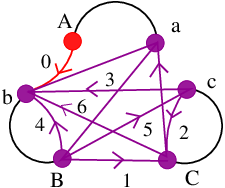
In Figure 20 we show the construction composition corresponding to the construction path of Figure 19. The source LTT structure of the switch is left out to highlight the fact that it does not affect the construction path.

We determine the sequence of LTT structures in the construction composition by attaching the red edge in to the terminal vertex of edge in the construction path. The generator can be determined by the red edge in its destination LTT structure: If the red vertex of is and the red edge is , then is defined by .
The following proposition tells us that construction paths are “built” by construction compositions. By saying a turn is taken by , we will mean that the turn is taken by some .
Proposition 7.25.
Let be an ideally decomposed Type (*) representative of with . Suppose that is decomposable as ,
with the sequence of LTT structures for :
.
Assume the Standard Notation for a Type (*) LTT Structure. If is a construction composition, then contains as a subgraph the purple edges in the construction path for .
Proof: We will proceed by induction for decreasing values. Since nothing in the proof will rely on (which is the only thing that distinguishes that is a switch instead of an extension), proof by induction is valid here.
For the base case consider . By the Corollary 5.16 proof, creates the red edge in . We know that is defined by : and for all . Thus, since , we know that . So and, since images of purple and red edges of are purple edges of , is a purple edge in . The base case is proved.
For the inductive step assume that, for , contains as a subgraph the purple edges in the construction path associated to . The red edge that creates in is (see the proof of Corollary 5.16). As above, is represented by a purple edge in . Since purple edges are always mapped to themselves by extensions and , , proving the inductive step. The proposition is proved.
QED.
7.4 Switch Paths
While they do not give insight into the progress of building and have more restrictions, switch sequences also have associated paths. The usefulness of switch paths lies in the aid they give in constructing the switch sequences required in our methods below. This subsection focuses on switch sequences and their associated switch paths.
We will continue in this section with the abuse of notation from the previous subsection (this mainly consists of ignoring second indices).
Definition 7.26.
A switch sequence for a Type (*) pIW graph is a pair
with a decomposition of as
,
and associated sequence of LTT structures
, where:
- (SS1)
-
each with is a permitted switch,
- (SS2)
-
for each , and
- (SS3)
-
and for all .
Sometimes we will just call a switch sequence when either the LTT structures should be clear from the decomposition or are unnecessary for discussion.
We call the composition of generators a switch sequence automorphism with source LTT structure and destination LTT structure .
Remark 7.27.
(SS3) is not implied by (SS1) and (SS2) and is necessary for a switch path to indeed be a path. Certain statements in the proof of Lemma 7.31 below (where we show that the switch path corresponding to a switch sequence is realized as a smooth path in the destination LTT structure) would be incorrect without (3).
Definition 7.28.
A realized switch sequence is a pair such that there exists an ideally decomposed Type (*) representative of having the sequence of LTT structures and satisfying that, for each , is a switch.
Again we call the composition of generators a switch sequence automorphism with source LTT structure and destination LTT structure .
Definition 7.29.
A switch path associated to a (realized) switch sequence is a path in the destination LTT structure for that starts with the red vertex , transverses the red edge [] for from the red vertex to the vertex , transverses the black edge [] from the vertex to the vertex , transverses what is the red edge [] = [] in (and a purple edge in ) from to , transverses the black edge [] from the vertex to the vertex , continues as such through all of the new red edges for the with , and ends by transversing the black edge [] from the vertex to the vertex and what is the red edge [] = [] in (purple edge in ), and then the black edge [] from the vertex to the vertex .
In other words, a switch path alternates between the red edges (oriented from the unachieved direction to ) for the (for descending ) and the black edges between.
Remark 7.30.
We clarify here some ways switch paths and construction paths differ.
- (1)
-
Switch paths look like construction paths but, while the purple edges in the construction path for a construction composition are purple in each with , for a switch path, they will be red edges in the structure they are created in and then will not exist at all in the structures with . The change of color of red edges and then disappearance of edges is the reason for (3) in the switch sequence definition.
- (2)
-
Unlike constructions paths, switch paths do not give subpaths of lamination leaves.
Lemma 7.31.
The switch path associated to a realized switch sequence forms a smooth path in the LTT structure .
Proof: The red edge in is []. We are left to show (by induction) that:
(1) For each , [] is a purple edge of and
(2) the purple edges [] (together with the black edges in the switch sequence) form a smooth path in .
Start with the base case. By the switch properties, the red edge in is []. Since and (by the switch sequence definition), . Thus, by Lemma 5.21, ], is a purple edge in . The red edge in is . So, by including the black edge [], we have a path in . This path is smooth since it alternates between colored and black edges. So our proof of the base case is complete.
We now prove the inductive step. By the inductive hypothesis we assume that the sequence of switches associated to gives us a smooth path in ending with a purple edge with “free” vertex . We know that the red edge in is ]. As long as we do not have or for (which holds again by the definition of a switch sequence), . This, as above, makes a purple edge in by Lemma 5.21.
Since is a smooth path in ending with a black edge,
is also a smooth path in , [] is a black edge in and as [] is a purple edge in .
QED.
Example 7.32.
We return to the LTT structure (for Graph XX) of Example 7.24 and number below the colored edges of a switch path.
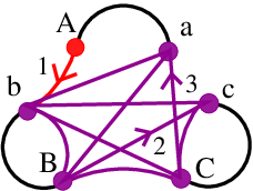
A switch sequence for constructed from the switch path is:

Notice how the red edge in the destination LTT structure for the generator labeled by (1) is the first colored edge in the switch path, the red edge in the destination LTT structure for (2) is the second colored edge in the switch path, etc.
8 AM Diagrams
In this section we describe how to construct the “AM Diagram” for a Type (*) pIWG, as well as prove that Type (*) representatives are realized as loops in these diagrams.
Definition 8.1.
Let be a given Type (*) pIW graph. A PreAdmissible Map Diagram (PreAM Diagram) for or ) is the directed graph where
- 1.
the nodes correspond to equivalence classes of admissible LTT structures for
- 2.
for each admissible generator triple (, , ) for , there exists a directed edge from the node [] to the node [].
The disjoint union of the maximal strongly connected subgraphs of will be called the Admissible Map Diagram for (or ).
The following proposition shows that we can restrict our search for representatives to loops in AM Diagrams. For the proposition and henceforth after, will denote the oriented edge from [] to [] labeled by and will denote the oriented path in from [] to [] that transverses the edges corresponding to the generators in the order they are composed (starting with the edge and concluding with the ). We say that realizes or that is realized by . In particular, we say that the decomposition of is realized by in .
Proposition 8.2.
If is an ideally decomposed Type (*) representative of such that , with corresponding sequence of LTT structures , then forms an oriented loop in .
Proof: Suppose that is such a representative. We showed in Proposition 7.15 that is a composition of permitted switches and permitted extensions , and thus of admissible maps. This tells us that forms an oriented loop in . Since all loops of a graph are contained in the union of the maximal strongly connected subgraphs of the graph, we know that is actually in , proving the proposition.
QED.
Definition 8.3.
We denote the loop by .
Corollary 8.4.
(of Proposition 8.2) If no loop in gives a Type (*) representative of an ageometric, fully irreducible outer automorphism such that , then such a does not exist. In particular, any of the following properties of an AM Diagram would prove that such a representative does not exist:
- (1)
There is at least one edge direction pair , where , such that no red vertex in is labeled by either or .
- (2)
The representative corresponding to each loop in has a PNP.
Proof: Proposition 3.3 says that such a would have an ideally decomposed Type (*) representative and Proposition 8.2 shows that any ideally decomposed Type (*) representative would be realized by a loop in . Thus, has a realization in .
If, for some , did not contain an LTT structure where either or , then the corresponding automorphism would fix the generator of corresponding to , which would make reducible, contradicting that is fully irreducible. So (1) is proved.
Since Type (*) representatives must be PNP-free, if no loop in realizes a PNP-free automorphism, then no Type (*) representative exists. This proves (2) and thus the entire corollary since the first sentence is a direct consequence of the Proposition 8.2.
QED.
9 Full Irreducibility Criterion
The main goal of this section is the proof of a “Folk Lemma” giving a criterion, the “Full Irreducibility Criterion (FIC),” for an irreducible train track map to represent a fully irreducible outer automorphism. Our original approach to proving the criterion involved the “Weak Attraction Theorem,” several notions of train tracks, laminations, and the basin of attraction for a lamination. However, Michael Handel graciously provided a way to finish the proof making much of our initial work unnecessary. The proof of the criterion we give here uses Michael Handel’s recommendation.
9.1 Free Factor Systems, Filtrations, and RTTs
The following definitions are necessary to understand the definition of a relative train track representative for an outer automorphism. While [BH92] gives that we always have train track representatives for irreducible outer automorphisms, this is not true for reducible outer automorphisms. Relative train tracks were invented by Bestvina and Handel to approximate train tracks as best possible in this circumstance. We use relative train tracks in our proof of the Full Irreducibility Criterion.
We begin by defining a “free factor system” for a free group, , of rank .
Definition 9.1 (BFH00).
is a free factor system for if is a free factor of and each is nontrivial. For free factor systems and , we say that when, for each , there exists some such that , i.e. is conjugate to a free factor of .
A distinguishing characteristic of reducible outer automorphism representatives is the existence of proper nontrivial invariant subgraphs. A relative train track representative of such an outer automorphism will have a “filtration” of invariant subgraphs “realizing” a nested sequence of free factors. Over the course of the next few definitions we describe what this means.
Definition 9.2 (BH92).
For a topological representative of , an increasing sequence of -invariant subgraphs such that each component of each subgraph contains at least one edge is called a filtration. For such a filtration, the closure of is called the stratum. Let denote the set of edges of with some prescribed orientation and let . The transition submatrix for the stratum is the square matrix such that, for each and , the entry is the number of times crosses over in either direction. Strata with zero matrices as their transition submatrices are called zero strata. Let denote the Perron-Frobenius eigenvalue for , i.e. the real eigenvalue of largest norm. Then is called exponentially growing (EG) if and a nonexponentially growing (NEG) if .
We are now ready for the relative train track representative definition, as defined in [BH92].
Definition 9.3 (BH92).
A Relative Train Track (RTT) Representative of an outer automorphism is a topological representative and filtration such that:
- (1)
-
Each is either the zero matrix or is irreducible;
- (2)
-
all vertices have valence greater than one; and
- (3)
-
each EG-stratum satisfies:
- (a)
for each edge , the first edge of is in ,
- (b)
is nontrivial for each nontrivial path having endpoints in , and
- (c)
is a t-legal path (i.e. contains each of its illegal turns) for each legal path .
- (a)
The following are needed for understanding the revised versions of RTTs used in proving the Full Irreducibility Criterion.
Definition 9.4.
Suppose is a marked graph and is a subgraph with non-contractible components . Then is called the free factor system realized by . A nested sequence of free factor systems is said to be realized by an RTT and filtration if each is realized by some . [BH92]
A topological representative and filtration are called reduced if each satisfies: For any and each -invariant free factor system such that , either or . [BFH00]
We will use a correspondence proved in [BFH00] between attracting laminations for an outer automorphism and the EG-strata of an RTT representative of : For each EG stratum of , there exists a unique attracting lamination (denoted by ) having as the highest stratum crossed by the realization of a -generic line. is called the EG-stratum determined by .
We will remind the reader of the definition of a revised version of a relative train track called a “complete split relative train track (CT).” These train tracks are defined by M. Feighn and M. Handel in [FH09]. However, we first give the definition of a “complete splitting.” Both these definitions are specialized definitions for the case of ageometric outer automorphisms (where there are, in particular, no closed PNPs).
Definition 9.5 (FH09).
A nontrivial path or circuit is completely split if it has a complete splitting, i.e. can be written as where
- (1)
each is either a single edge in an irreducible stratum, an iNP, or a taken connecting path in a zero stratum and
- (2)
.
In the case of a complete splitting we write .
Definition 9.6 (FH09).
An RTT representative of , together with its filtration given by , is a Completely Split Relative Train Track (CT) if it satisfies all of the following:
- (CT1)
-
is rotationless.
- (CT2)
-
is completely split, that is:
- (a)
is completely split for each edge in each irreducible stratum and
- (b)
is completely split for each taken connecting path in a zero stratum.
- (a)
- (CT3)
-
is reduced and the cores of the are also filtration elements. (Recall that the core of a finite graph is the subgraph consisting of all edges of crossed by some circuit in ).
- (CT4)
-
The endpoints of all iNPs are vertices (necessarily principal). For each NEG-stratum and nonfixed edge of , the terminal endpoint is principal (and hence fixed).
- (CT5)
-
Periodic edges are fixed and the endpoints of fixed edges are principal. For a fixed stratum with unique edge , either is a loop or each end of is in and is a core graph.
- (CT6)
-
For each zero stratum , there is an EG-stratum (with ) such that:
- (a)
is enveloped by , i.e.
- (i)
for some , is irreducible,
- (ii)
no component of is contractible,
- (iii)
is a component of , and
- (iv)
each -vertex is of valence greater than one in .
- (i)
- (b)
Each edge of is -taken (i.e. is a maximal subpath of in for some and edge in )
- (c)
contains every vertex of and the link of each vertex of is contained in .
- (a)
- (CT7)
-
There are no linear edges (i.e. edges of NEG-strata such that for some nontrivial NP ).
- (CT8)
-
The highest edges of iNPs do not belong to NEG-strata.
- (CT9)
-
Suppose that is an EG-stratum and that is a height- iNP. Then the restriction of to is where:
- (a)
can be decomposed into proper extended folds defined by iteratively folding ,
- (b)
can be decomposed into folds involving edges in , and
- (c)
is a homomorphism.
- (a)
Remark 9.7.
If is forward rotationless and is a nested sequence of -invariant free factor systems, then is represented by a CT and filtration that realizes [FH09, Theorem 4.29].
Before we can finally give our Fully Irreducibility Criterion proof, we need to remind the reader of the following.
Definition 9.8 (BFH00).
The complexity of the free factor system is defined to be zero if is trivial and is otherwise defined to be the non-increasing sequence of positive integers obtained by rearranging the set . The set of all complexities is given a lexicographic ordering.
The free factor support for a subset is defined in [BFH00, Corollary 2.6.5] to be the unique free factor system of minimal complexity carrying every element of .
The only relevant information about the free factor support for our proof of the FIC is that, if a lamination is carried by a proper free factor, then its support is a proper free factor. If this were not the case, then the free factor support would have to have rank (and thus complexity ), while the free factor carrying the lamination (because it is proper) must be of rank less than , giving it complexity less than the free factor support and hence contradicting that a free factor support is of minimal complexity.
We would like to credit Michael Handel for his contributions to the proof of the following “Folk lemma,” which we will call the Full Irreducibility Criterion (FIC).
Lemma 9.9.
(The Full Irreducibility Criterion) Let be an irreducible train track representative of . Suppose that
- (I)
has no PNPs,
- (II)
the transition matrix for is Perron-Frobenius, and
- (III)
all for are connected.
Then is a fully irreducible outer automorphism.
Proof: Suppose that is an irreducible TT representative of with Perron-Frobenius transition matrix, with connected local Whitehead graphs, and with no PNPs. Since has a Perron-Frobenius transition matrix, as an RTT, it has precisely one stratum and that stratum is EG. Hence, it has precisely one attracting lamination [BFH00]. Since the number of attracting laminations belonging to a TT representative of is independent of the choice of representative, any representative of would also have precisely one attracting lamination.
Suppose, for the sake of contradiction, that were not fully irreducible. Then some power of would be reducible. If necessary, take an even higher power so that will also be rotationless (this does not change the reducibility). Notice that, since is -invariant, any representative of would also have precisely one attracting lamination.
Since is reducible (and rotationless), there exists a completely split train track representative of with more than one stratum [FH09, Theorem 4.29]. Since has precisely one attracting lamination, will have precisely one EG-stratum . Each stratum , other than and any zero strata (if they exist), would be an NEG-stratum consisting of a single edge [FH09, Lemma 4.22]. We will consider separately the cases where and where .
Notice that, since any zero stratum has zero transition matrix (and thus must have every edge mapped to a lower filtration element by ), a zero stratum could not be . Thus, if , then is NEG and must consist of a single edge . Since is bottom-most, it would have to be fixed, as there are no lower strata for its edge to be mapped into. But then, according to (CT5), would have to be an invariant loop, which would mean that would have a rank-1 invariant free factor. However, was PNP-free, which means that was PNP-free and thus that should not be able to have a rank-1 invariant free factor. We have thus reached a contradiction for the case where .
Now assume that . This would imply that is carried by a proper free factor. Proposition 2.4 of [BFH97] states that, if a finitely generated subgroup carries , then has finite index in . The necessary conditions for this proposition are actually only: (1) the transition matrix of is irreducible and (2) at each vertex of , the local Whitehead graph is connected. (Up to the contradiction in the proof of Proposition 2.4 of [BFH97], the only properties used in the proof are that the support is finitely generated, proper, and carries the lamination. The contradiction uses Lemma 2.1 of [BFH97], which simply proves that properties (1) and (2) carry over to lifts of to finite-sheeted covering spaces, using no properties other than properties (1) and (2).) The assumptions (1) and (2) are assumptions in the hypotheses of our criteria and is still the attracting lamination for and so we can apply the proposition to create a contradiction with the fact that has proper free factor support. Applying the proposition, since proper free factors have infinite index, the support must be the whole group. This contradicts that the EG-stratum is and that there must be more than one stratum.
We have thus shown that we cannot have more than one stratum with or . So all powers of must be irreducible and thus is fully irreducible, as desired.
QED.
Remark 9.10.
To apply this lemma, we need a procedure for proving the nonexistence of PNPs, as stated in Proposition 10.2 of the following section.
10 Nielsen Path Identification
In this section we give a method for finding all iPNPs, thus PNPs, in our circumstance. While we have not yet proved the method’s finiteness, its application ended quickly in all examples thus far.
Example 10.1.
As a warm-up to the procedure, we give the following example of the procedure applied to the construction composition :
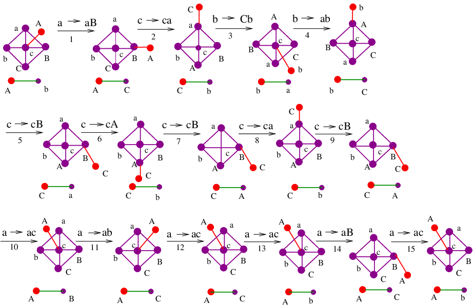
The green illegal turn for is . We will try to build an iPNP where and are legal paths.
Since is a subpath of , we must add another edge after in . And, since is red in , the edge added after will be such that its initial direction is a preimage of (the other direction in ) under . The only such preimage is . Thus, the next edge of would have to be .
is a subpath of , so we must add another edge after in . Since is red in , the edge added after will be such that its initial direction is a preimage of (the other direction in ) under . There are two such preimages: Case 1 will be where the initial direction is and Case 2 will be where the initial direction is .
We try each of these as the next edge of .
For Case 1, suppose that the next edge of is . Since is a subpath of , it follows that we must add another edge after in . Since is red in , the new edge will have to be such that its initial direction is a preimage of (the other direction in ) under . The only such preimage is . So the next edge of would have to be .
Now, and . Since (and ), and could not start and , respectively.
For Case 2, suppose that the next edge of is . Since is a subpath of , it follows that we must add another edge of after . As above, is red in , so we can follow the logic above and see that the next edge of would have to be .
and , which again leaves us with . So, as above, and could not start and , respectively.
This rules out all possibilities for and so has no iPNPs, and thus no PNPs, as desired.
Throughout this section, will be a semi-ideally decomposed TT representative of with the same notation as that given at the end of Section 3. We will additionally require that satisfies AM Properties (I)-(VIII) and, in particular, is a permitted composition. Let and .
Proposition 10.2.
There exists a procedure for determining all iPNPs for , where ; ; ; and is the unique illegal turn of .
Let and throughout the following procedure.
- (I)
-
Apply generators , , etc, to and to until . Either is a subpath of or vice versa. Without loss of generality assume that is a subpath of so that , for some edge . (Otherwise just switch all and , and , etc, in the following arguments). Then, must contain another edge .
We explain in (III) how to find all possibilities for this edge. - (II)
-
Inductively, assume that (or again switch for , for , and so on).
- (III)
-
We must add another edge to . There are two cases to consider:
- (a)
If , then the different possibilities for are determined by the directions such that where . (In this case there is a green segment between and in , and is the non-red direction of ).
- (b)
If , then the different possibilities for are all edges such that where .
After throwing out any choices for such that is the green illegal turn for , each remaining in (a) or (b) gives another prospective iPNP that we must continue applying the algorithm to.
- (a)
- (IV)
-
Suppose that at some step we do not have that is a subpath of (or vice versa). Then we compose with generators until either:
- (a)
We composed with enough to obtain some such that and for some legal path (in this case proceed to (V) ),
- (b)
is a subpath of or vice versa (in this case, return to (II) and continue with the algorithm as before), or
- (c)
some and where is a legal turn in . In this case there cannot be an iPNP with as a subpath (proceed to (VIII)).
- (a)
- (V)
-
For each such that and for some legal path (for the appropriate m and n), check if or vice versa and follow the appropriate step (among (a)-(d) below).
- (a)
If, for some , , then is the only possible iPNP for .
- (b)
For each such that (where containment is proper), proceed to (VII).
- (c)
If (where containment is proper), proceed to (VI).
- (d)
If we do not have or vice versa for any , then there is only one circumstance where we can possibly have an iPNP with as a subpath. This is the case where where either and or and . In this case, apply (VII) to the side that is too short. Otherwise, there cannot be an iPNP with as a subpath, so proceed to (VIII).
- (a)
- (VI)
-
We assume here that . Consider the final occurrence of in the copy of in and the final occurrence of in the copy of in . This final occurrence of must have come from and this final occurrence of must have come from . This means that we have fixed points in and . Replace with where is the same as , except that and are replaced with some partial edges ending at the fixed points. Repeat this process until some is an iPNP.
- (VII)
-
We assume here that (where containment is proper). Without loss of generality, assume that there exists a such that . For each direction such that and such that is not the green illegal turn for , return to (V) with where .
- (VIII)
-
Continue to rule out the other possible subpaths that have arisen via this procedure (by different choices of , as in (III) or (VII)). If there are no other possible subpaths, then we have shown there are no iPNPs for , and thus no PNPs for .
We will need the following Lemma(s) for the proof of this proposition.
Lemma 10.3.
Subpaths of legal paths are legal.
Proof of Lemma: The set of turns of the subpath is a subset of the set of turns of the path. Since all turns of the path are legal, all turns of the subpath must also be legal. So the subpath must also be a legal path.
QED.
Proof of Proposition: We begin with an argument that will be used throughout the proof. Since is an iPNP, and are both legal paths. Since subpaths of legal paths are legal and since the images under of legal paths are legal, the paths and are legal for each , , and .
Since is an illegal turn, for some , . We need to prove that either is a subpath of or vice versa. Let and . Since is an illegal turn for and the only illegal turn for is , . Without loss of generality suppose that (and ). Since is defined by , it follows that and . So is a subpath of . Since is an automorphism and also takes legal paths to legal paths, is a subpath of , as desired.
The final thing to show for (I) is that must contain a second edge . Suppose did not contain a second edge. Then tightening would cancel out all of with an initial subpath of and so certainly would cancel out all of with an initial subpath of . Thus, would be a subpath of and hence would be legal. So is legal for all , contradicting that some , which has an illegal turn.
To start off proving (III) we need a similar argument, as in the previous paragraph, to show that would have to have another edge . For the sake of contradiction, suppose that ended with . Then would be a subpath of (for similar reasons as above), which leads to a contradiction as in the argument above.
We now prove the claims of (IIIa) and (IIIb). Since ,
for some legal path ( is legal because it is a subpath of the image of the legal path ). Additionally, will be legal since is a legal path. Thus, , which is just unless , and then is legal unless is an illegal turn, i.e. with .
Suppose first that (as in (III)(a)). Notice that, in this case, is not in the image of and thus is not in the image of and so . This tells us that , which will be a legal path unless . However, if ) , then
, since and are legal paths and the images of edges are legal. But is a subpath of , so is legal, and is a subpath of , so is legal, and we still have that is legal, which together would make legal. This contradicts that some must be , which has an illegal turn. So, , as desired.
Suppose now (as in (III)(b)) that . For the sake of contradiction suppose that , where . First off, notice that this means that again . Also, since cannot be (see reasoning above) and , we cannot have . This would make legal, which leads to a contradiction as above. So , as desired.
The final observation about (III) is that choices for such that must be thrown out since must be a legal path.
We need to show for (IVc) that, if and where is a legal turn in , then there cannot be an iPNP with as a subpath. We prove this now. Under the stated conditions, and where is an initial subpath of (both of which are legal) and is an initial subpath of (both of which are legal). Since is a legal turn, , which is a legal path. Let be such that . (Without loss of generality we can assume that by replacing by a multiple of if necessary). Then, , since is a legal path. This makes legal since images under permitted compositions of legal paths are legal. And this contradicts that , which is not a legal path. We have now verified everything needing verification in (IV).
As in (V), suppose that and for some legal path (for the appropriate and ). (Va) is true by definition. Since (Vb) and (Vc) just refer us to later steps, we can just focus on (Vd) for now. The first thing that we need to prove for (Vd) is that there is only one circumstance where we can possibly have an iPNP with as a subpath. Suppose that, for no power do we ever have , , , or where either and or and . Now, for the sake of contradiction, suppose that some containing is an iPNP of period . Since is an iPNP, and are both legal paths (as are the subpath and ). This tells us that . So . But this lands us in one of the situations we said could not occur, which is a contradiction.
The verification of (VI) is left to the reader and there is nothing really to prove in (VII) since the conditions for (V) still hold.
QED.
11 Representative Loops
The goal of this section is to prove, for a Type (*) pIW graph , that representatives coming from the loops in the and satisfying certain prescribed properties, as mentioned before, are indeed TT representatives of ageometric, fully irreducible such that . This result is given in Proposition 11.4.
The following three lemmas are used in the proof of Proposition 11.4.
Lemma 11.1.
For each , is not represented by any edge in .
Proof: For the sake of contradiction suppose that were represented by an edge in . Then would be a turn in some . By Lemma 5.2, the edge path contains . Thus, the edge path would also contain the turn . Since , this would contradict that cannot have cancelation. So cannot be represented by any edge in , as desired.
QED.
Lemma 11.2.
Since one vertex of the green illegal turn of will be , cannot also be a purple edge in . Also, must be a vertex of the red edge of .
Proof: Since has no preimage under , it cannot be a vertex of a purple edge of , as the purple edges of are images of purple and red turns of under . The red edge in is , which contains .
QED.
Lemma 11.3.
For permitted compositions, images of legal paths and turns are legal.
Proof of Lemma: Suppose that is a legal path and suppose that is a permitted composition. Since permitted compositions are train track maps, the image under of any edge of is legal. Thus, we only need to be concerned about what happens with the turns of . Since is legal, all turns of are legal. Since images of legal turns are legal, the images of all turns of are legal. Thus, the image of is legal, as desired.
QED.
Proposition 11.4.
Suppose that is a Type (*) pIW graph and that is a loop in satisfying:
-
1. Each purple edge of correspond to a turn taken by some where ;
-
2. for each , there exists some such that contains either or ; and
-
3. has no periodic Nielsen paths.
Then is a train track representative of an ageometric fully irreducible such that .
Proof of Proposition: By the FIC, we only need to show that is a train track map, the transition matrix of is Perron-Frobenius, and . Property (2) of this proposition is the same as AM Property (VIc) and so that the transition matrix is Perron-Frobenius follows from Lemma 6.1. That is a train track map follows from Lemma 6.1. Since has no PNPs, , where . By the definition of , edges correspond precisely with turns crossed over by some were . By the definition of the edges of correspond precisely with the purple edges of .
This completes the proof.
QED.
12 Procedure for Building Ideal Whitehead Graphs
In this section we give three different methods for constructing train track representatives that have the potential to be of Type (*) with a Type (*) pIW graph ideal Whitehead graph . Different methods work better in different circumstances. For example, if most of the LTT structures with are birecurrent, then Methods II and III are better suited (as may be very large and impractical to construct). On the other hand, if only a few of the LTT structures with are birecurrent, then constructing is much simpler than using “guess and check” methods and so Method I generally proves more practical.
In all figures of this section we continue with the convention that Y denotes , etc.
12.1 Method I (Building the Entire AM Diagram)
Let be a Type (*) pIW graph. We explain in Steps 1-6 below a procedure for constructing . Once has been built, one still needs to find an appropriate loop in . We explain how to do this in Step 7. The final step will be to test the representative constructed from the loop to ensure that it is PNP-free. The procedure for identifying PNPs was explained and proved in Section 10.
STEP 1: CONSTRUCT AN LTT CHART FOR
- A.
-
An LTT Chart for will contain precisely one column for each way of labeling the vertices of with , except that:
- 1.
We consider labelings of the vertices of equivalent when there is a permutation of the indices and a permutation of the two elements of each pair making the labelings identical (when we have such a permutation, we say that the labeled graphs are Edge Pair Permutation (EPP) Isomorphic, even in a graph where we also have a vertex labeled by or include black edges, making the graph an LTT structure)
Example 12.1.
The following are two EPP-isomorphic graphs (in this example and the following examples, denotes , denotes , denotes , denotes , denotes , and denotes ):

Figure 24: Graphs EPP Isomorphic by the permutation taking to and to - 2.
We leave out any labeling causing to have two edges of the form , each with a valence-one vertex (we will call an edge containing a valence-one vertex a valence-one edge and a pair of vertices of the form an edge pair, making the statement say that we leave out any labeling causing to have two distinct pairs of edge-pair labeled vertices, each connected by a valence-one edge).
Example 12.2.
Here we show a graph not included as a result of having distinct pairs of edge-pair labeled vertices, each connected by a valence-1 edge.

Figure 25: Not in LTT Chart since and valence-one edges
- 1.
- B.
-
Graphs determining the columns of an LTT Chart are colored purple and labeled from left to right by , , etc. We call these graphs the Determining SW-Graphs for the columns.
Remark 12.3.
There is no canonical way of ordering the graph that will be , , etc. There is also no canonical way of choosing a labeled graph representing an EPP-isomorphic equivalence class. Thus, there will be multiple possible LTT Charts for , all of which will lead to the same diagram .
Example 12.4.
In the case of Graph VII, one set of representatives we could use to determine the columns would be:

Figure 26: Determining SW-Graphs for Graph VII - C.
-
Each column of the LTT Chart will contain a graph for each way of attaching (at a single vertex, called the attaching vertex) a red edge to the column’s determining SW-graph so that:
- 1.
the valence-one vertex of the red edge (which is colored red and called the free vertex) is labeled by and
- 2.
no valence-one edge connects edge pair vertices (there are no edges of the form where either has valence one or has valence one).
Example 12.5.
We show here two graphs that would not be included in an LTT Chart for Graph VII because they each have a valence-one edge connecting edge-pair vertices.

Figure 27: Graphs not in LTT Chart because and are valence-one edges
- 1.
- D.
-
We label graphs in the first () column from top to bottom , , , ; graphs in the second () column from top to bottom , , , ; etc.
Example 12.6.
An LTT Chart for Graph VII
In the following chart, the graphs we leave out are either EPP-isomorphic to one among those we included (see Figure 24) or violate one of the conditions for inclusion (as in Figure 27). We continue to denote by , we denote by , we denote by , we denote by , we denote by , and we denote by .

STEP 2: BIRECURRENCY
For each graph in the LTT Chart for , and each , add a black edge connecting and (notice that the graphs are now smooth train track graphs). Check each of these graphs for birecurrency, put a box around each birecurrent graph in the LTT chart, and cross out each nonbirecurrent graph in the LTT chart.
Example 12.7.
Birecurrency for Graph VII
We leave out here labels on the vertices of each LTT structure to highlight that the only significant information is vertex color and whether two vertices are part of an edge pair (forming an edge pair with the free vertex will have added significance). The fact that black edges connect edge-pair vertices encodes the information needed.

From the above figure one can see that the only LTT chart graph with a birecurrent LTT structure is IVe. We cross out and “box” the corresponding graphs in the LTT Chart to get:

STEP 3: A PERMITTED EXTENSION/SWITCH WEB
Consider the LTT structure for any boxed graph from the LTT chart. In what follows, for each , will be used to denote both and . The attaching vertex of (the purple vertex of the red edge of ) will be denoted by (the “a” here is for “attaching”). Additionally, in the figures, we will use to denote .
- A.
-
We determine all permitted extensions and permitted switches with as their destination LTT structure (i.e. ).
- 1.
-
Remove the interior of all black edges from to retrieve the colored subgraph , called the CLW-graph for , from the LTT chart.
- 2.
-
For each vertex distance-one in from we determine two potential “ingoing LTT Structures” (a switch and an extension). In LTT structure notation (where ), is denoted and the label on the free vertex is denoted .
- (a)
Associated to the distance-one vertex , the potential ingoing extension graph, , will have:
- –
the same purple subgraph as that of
- –
the second index of the label on the free vertex will remain the same, i.e. and, if we use the same letters to label the vertices in and , the same letter remains on the free vertex
- –
the red edge will now be attached at , instead of at

Figure 31: Potential Ingoing Extension Graph for : Notice that the label on the free vertex remains the same () but that the attaching vertex of the red edge changes from () to the distance-one vertex . - –
- (b)
The potential ingoing switch graph, , will have an isomorphic purple subgraph to that of . The labeling is almost the same labeling except that the second index of in is the second index of the vertex in that is mapped by the isomorphism to the vertex labeled with . (If we use the same letters to label the vertices in and , it will look as if the label on the red vertex in has moved to the position in of what had been in (the inverse of the attaching vertex)).
- –
The label on the red vertex in is .
- –
The red edge in is attached at .
- –
The label on the free vertex is now .
- –

Figure 32: Potential Ingoing Switch Graph for : Notice how the purple graph with its labels looks the same except for movement of and . Also notice how the red edge shifts. - (a)
- 3.
-
Construct in this way the CLW-graph for each potential ingoing LTT structure corresponding to each vertex that is distance-one in from .
- 4.
-
Label each CLW-graph and with the label of the LTT Chart EPP-isomorphic graph(labels will be of the form ).
- 5.
-
If a CLW-graph is not EPP-isomorphic to a graph in the LTT Chart (i.e. if there is an edge of the from where either or has valence-one), cross it out. Also cross out any graph EPP-isomorphic to a graph crossed out in the LTT chart.
- 6.
-
Each remaining potential ingoing LTT structure CLW-graph, , will be EPP-isomorphic to a graph with a box around it in the LTT Chart. Box the label of the graph in the web and draw an arrow in the web from each such to .
- 7.
-
We now have a graph with a number of arrows entering it. Each arrow originates at a potential ingoing LTT structure CLW-graph that is labeled with the label of the EPP isomorphic boxed graph in the LTT chart. The label of each of these is boxed in the web. If some has the same LTT Chart label as , we box the entire graph in the web. Such a boxed graph will be called a branch end.
- 8.
-
For each potential ingoing LTT structure CLW-graph for with a box around its label, carry out the same procedure to find all of its potential ingoing LTT structure CLW-graphs, their labels, whether they have their labels boxed, and their arrows.
- •
In this stage (and all subsequent stages), box graphs (not crossed out) EPP-isomorphic to graphs that have already occurred elsewhere in the web. Such boxed graphs are again called branch ends and do not need their potential ingoing LTT structures determined (as they are determined elsewhere in the web).
- •
- 9.
-
Continue this process recursively.
- 10.
-
When the recursion ends (see Remark 12.8 for why it must end), one portion of the web is complete. This process will be repeated to create further portions that will need to be glued together in the end:
- (a)
If there is some boxed graph in the LTT chart not EPP-isomorphic to any graph in the portion of the web obtained by starting with , then use any such to start the construction of another portion of the web in the same way we constructed the portion starting with .
- (b)
Keep constructing portions of the web as such until all boxed graphs in the LTT chart have arisen in at least one portion of the web constructed.
- (a)
Remark 12.8.
The recursion process ends, as the LTT chart is finite (so there are a finite number of “portions” of the web) and a branch can only contain each LTT Chart element once.
Remark 12.9.
A refined version of the web could be obtained by gluing together distinct pieces of the web at graphs that are both the starting graph of one piece and (up to EPP-isomorphism) a branch end in a separate piece. If the graphs glued are only EPP-isomorphic (and not identical), this would also involve an EPP isomorphism of one of the entire pieces glued (this is possible since we are never gluing a piece to itself). None of this refinement is necessary to properly perform the remaining steps of Method I and so one can just leave their web in a nonminimal number of pieces.
Example 12.10.
A Permitted Extension/Switch Web for Graph VII
Above we saw that the only LTT chart graph with a birecurrent LTT structure is IVe. and so the distance-1 vertices are those labeled , and . We get four potential ingoing extension graphs by attaching the red edge to each of these four vertices. However, the only one having a birecurrent LTT structure is that where the red edge was not moved (and thus is still attached to the vertex labeled ). Therefore, the only permitted ingoing extension is the self-map of IVe. To get the four potential ingoing switch graphs for IVe, we again attach the red edge to each of the four vertices , and , but this time also switch the labels so that the free vertex is labeled and what was labeled before is now labeled . The only of these potential ingoing switch graphs having a birecurrent LTT structure is the one EPP-isomorphic to IVe, i.e. the one where the attaching vertex is . Thus, the Permitted Extension/Switch Web looks like:

STEP 4: THE (REFINED) SCHEMATIC EXTENSION/SWITCH WEB
Construct a directed graph from the information in the Permitted Extension/Switch Web by drawing:
- •
a vertex for each boxed graph in the LTT chart labeled as the boxed graph in the LTT chart is labeled
- •
a directed edge from a vertex of to a vertex of for each arrow in the web of Step 3 pointing from a graph with the labeling of to a graph with the labeling of .
Remark 12.11.
Notice that this schematic web is missing information about an edge pair permutation that may occur in its loops, but we currently do not need that information and can/will retrieve it from the web of Step 3 when necessary.
Before proceeding we trim the schematic web, leaving only its maximal strongly connected components. This can be done by inductively removing any vertex with no colored edges entering it as well as removing the interiors of edges that exit a removed vertex. We call this “trimmed” web a Refined Schematic Extension/Switch Web and denote it here by .
Example 12.12.
(Refined) Schematic Extension/Switch Web for Graph VII
Since we have precisely a single extension and switch mapping IVe to itself, the Schematic Permitted Extension/Switch Web is just:

There was no trimming necessary to find the maximal strongly connected subgraph. Thus, the Schematic Refined Permitted Extension/Switch Web is the same.
STEP 5: ILLUSTRATIVE AM DIAGRAM
The illustrative AM Diagram, , for a Type (*) pIW graph is constructed as follows:
- (A)
-
Choose some vertex in the Refined Schematic Web . Let be the graph in the LTT chart labeled the same as .
- (B)
-
Build the corresponding LTT Structure from by adding a black edge to for each set of edge-pair vertices in .
- (C)
-
For each directed edge entering in there will be an arrow in entering .
- (D)
-
To determine the LTT structures at the initial ends of the arrows entering :
-
1. Find the corresponding arrow in the web of Step 3.
-
2. If the terminal LTT structure in the web differs from by an EPP-isomorphism, apply the permutation of vertex labels realizing from to the arrow’s initial LTT structure in the web will give the appropriate initial structure for the arrow in the illustrative AM Diagram.
-
3. If , include only one copy of , drawing the arrow as a loop.
-
4. Differentiate between different EPP-isomorphic graphs and include them separately when they occur.
-
- (E)
-
Label all arrows terminating at by where the red vertex of is labeled by and the red edge of is .
- (F)
-
For each initial LTT structure for each arrow constructed thus far, carry out the same process as was carried out for in (D) and (E). However, in no step should the same LTT structure be drawn twice. If the initial LTT structure for an arrow is already in the diagram just start the arrow at the copy of the LTT structure already in the diagram.
- (G)
-
Recursively follow this process until every structure in the diagram has the same number of arrows entering it as the corresponding vertex in the schematic diagram had entering it. If the schematic web had more than one component, the whole process must be carried out for each component of the schematic web. (Several components in the schematic web may end up as part of the same component in the if components of the schematic web were not glued in every possible circumstance.)
Example 12.13.
Illustrative AM Diagram for Graph VII
By referencing information in the full permitted extension/switch web we can obtain the illustrative AM Diagram. (There are more components, but each is the same up to EPP-isomorphism, so we show here only a single component.) Recall that the red edges determine the maps labeling the arrows.

STEP 6: THE AM DIAGRAM
is obtained from by
- (1)
-
replacing LTT Structures with nodes (labeled by those LTT structures they replaced) and
- (2)
-
replacing the arrows with directed edges (the maps in are the labels on the directed edges in ).
Example 12.14.
AM Diagram for Graph VII
This is only a single component of the diagram, but including one component suffices to understand the entire diagram, as the others are all the same up to EPP-isomorphism.

STEP 7: FINDING
- (A)
-
Check Irreducibility Potential: Check whether, in each connected component of , for each edge vertex pair , there exists a node in the component such that either or labels the red vertex in the LTT structure labeling the node. There needs to be at least one component where this holds and we only needs to check for in such components. If there is no component for which it holds, then we have shown that the graph is unachievable.
Example 12.15.
AM Diagram for Graph VII
We return to the AM Diagram for Graph VII given in Figure 36. Since contains only red vertices labeled and (and thus leaves out the edge vertex pair ) unless some other component contains all three edge vertex pairs (, , and ), Graph VII would be deemed unachievable at this stage. Since no other component does contain all three edge vertex pairs (all components are EPP-isomorphic), the analysis has led us to the conclusion that Graph VII is indeed unachievable. (We will later use these same arguments to deem Graph V unachievable.)
- (B)
-
To clarify the discussion here, we refer to the AM Diagram for Graph II.
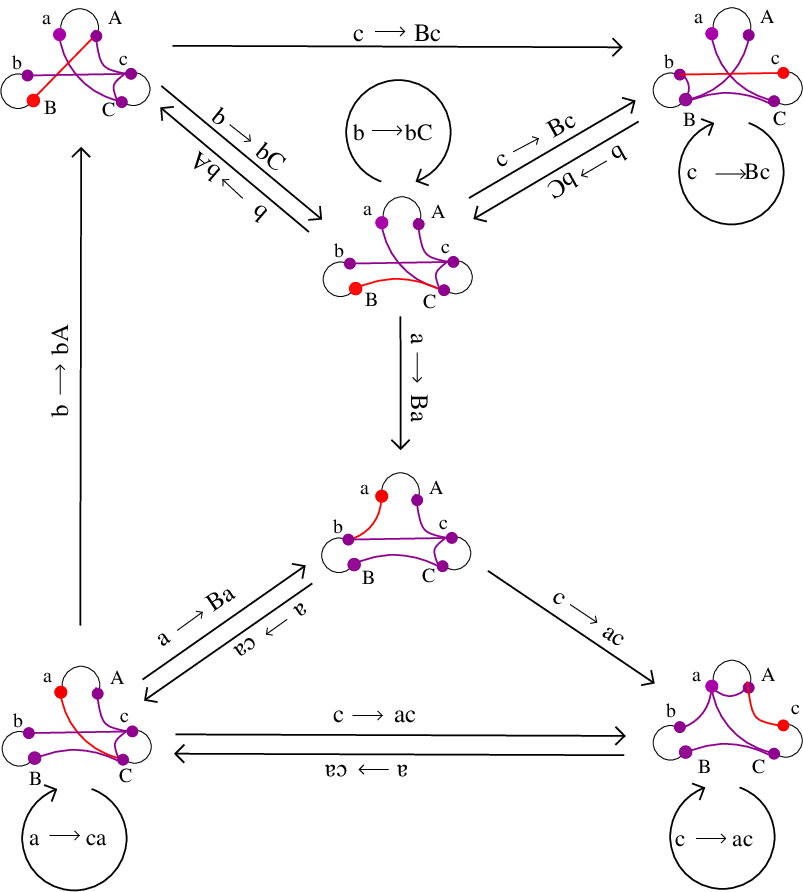
Each directed edge in corresponds to either a switch or an extension. Consider the subdiagram of consisting precisely of the directed edges corresponding to extensions (and their source and destination LTT structure nodes).

Notice that all of the LTT structures (source and destination LTT structures for the extensions) labeling nodes in a connected component of share the same purple subgraph (including the same labels on vertices). We call this purple subgraph the potential composition PI subgraph for the component.
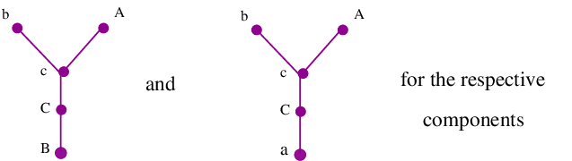
If we add black edges connecting edge pair vertices in the potential composition PI subgraph and then recursively remove any valence-one edges (leaving the vertex with valence greater than one each time we remove a valence-one edge), we get the potential composition subgraph for the connected component of .
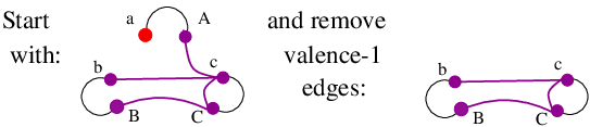
A directed smooth path (where the potential composition subgraph is viewed as a subgraph of an LTT structure ) is called a potential composition path.
Example 12.16.
We give here an example of a potential composition path.
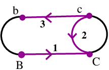
- (C)
-
There are multiple techniques for finding . Here are several:
- (1)
One can use potential composition paths to build portions of the graph (following progress using preimage subgraphs), see Method III.
- (2)
One can test the TT map corresponding to a loop in for being PNP-free, having Perron-Frobenius transition matrix, and having . If such is not the case, one can “attach” small loops to the initial loop in until the map satisfies those three necessary properties. If , the small loops attached can be determined by potential composition paths to ensure inclusion of necessary remaining edges (keeping in mind that the direction map will map purple edges of the construction path into the destination LTT structure).
- (1)
Example 12.17.
In this example we look at how to find a representative for Graph I. We start with the AM Diagram:

We find a loop to test in :
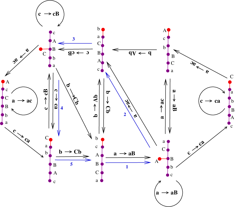
The loop gives:
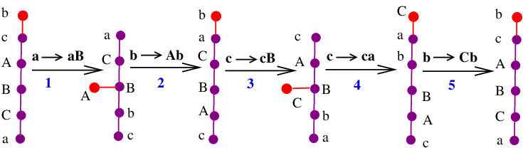
Since, the loop is not enough (we do not get the edge ), we add a second loop to it:
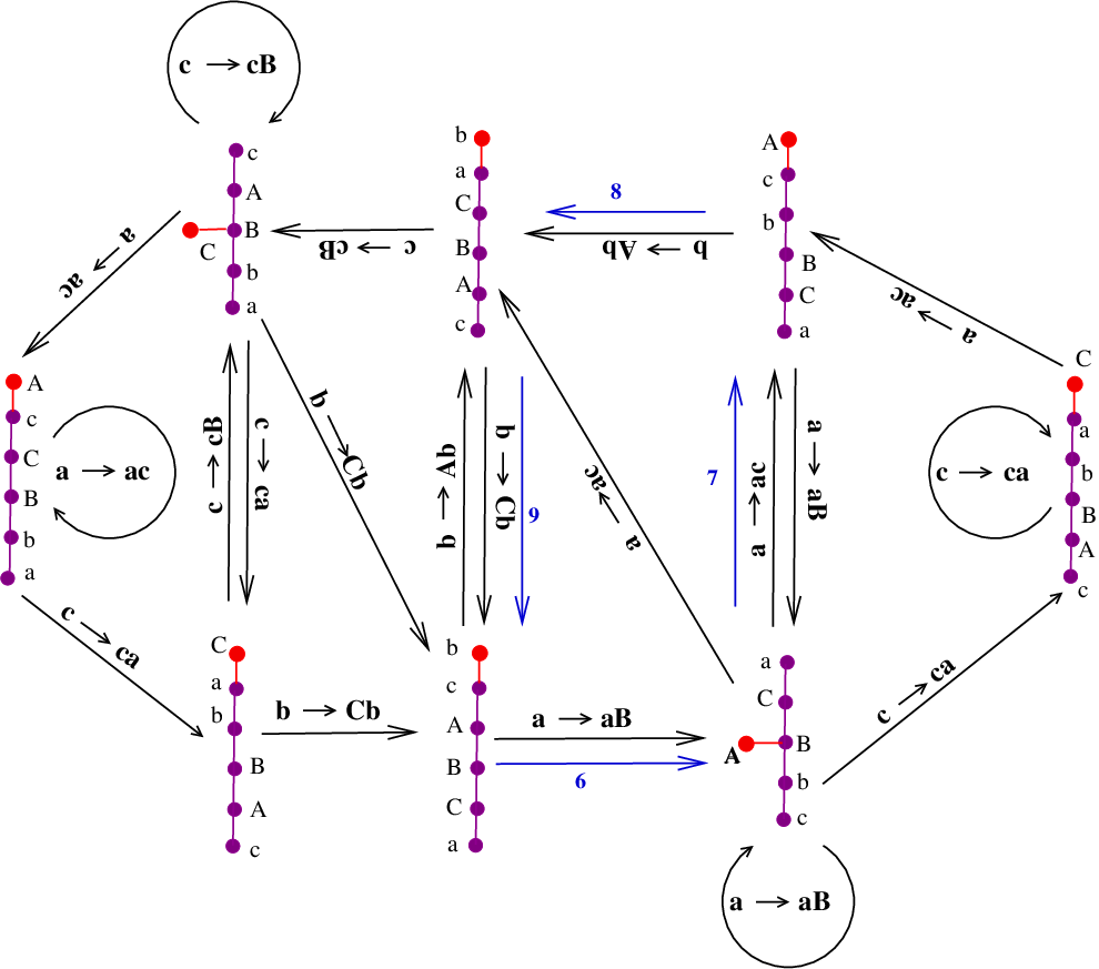
The loop gives:
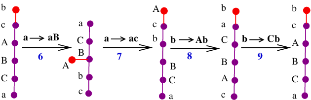
Combining the two loops we get the representative yielding Graph I (the line):
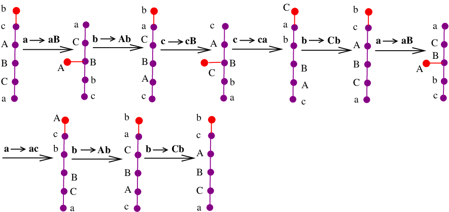
STEP 8: FINAL CHECKS
We need to check that:
- (1)
There are fixed directions.
- (2)
The map constructed is PNP-free.
- (3)
It is also important to check that the entire Type (*) pIW graph is “built.” We can do this by looking at the graph that is the union of the .
Example 12.18.
We show here an example of how to check that the entire Type (*) pIW graph is “built” (we iteratively take the image under each of the edges “created” thus far):
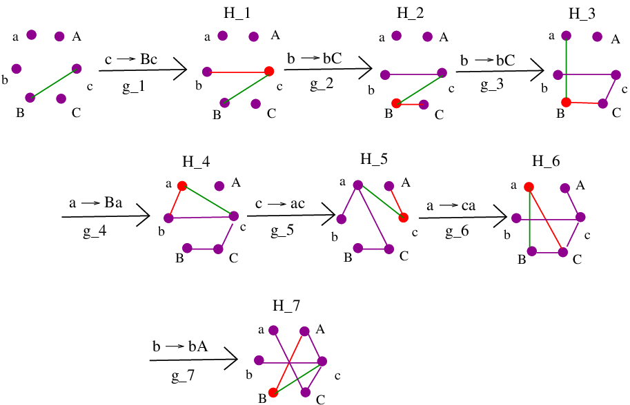
Figure 48: “Graph Building” We include subgraphs of the LTT structures to track how edges are “built.” The first generator is defined by . Thus, the red edge in the destination LTT structure for will be , where the red periodic direction vertex is labeled . The second generator is defined by . Thus, the red edge in the destination LTT structure for will be , where the red periodic direction vertex is labeled . This LTT structure will also contain the image of the red edge under the direction map . The third generator is defined again by . Thus, the red edge in the destination LTT structure for will be again , where the red periodic direction vertex is labeled . This LTT structure will also contain the image of the red edge and the image of the purple edge under the direction map . The fourth generator is defined by . Thus, the red edge in the destination LTT structure for will be , where the red periodic direction vertex is labeled . This LTT structure will also contain the image of the red edge and the images and of the purple edges and under the direction map . The remaining are constructed in a similar fashion.
12.2 Method II
Again let be a Type (*) pIWG. And let be a Type (*) admissible LTT structure with and the standard Type (*) admissible LTT structure notation.
Definition 12.19.
will denote the subgraph of containing all construction paths corresponding to construction compositions with destination LTT structure .
STEP 1: FIRST BUILDING SUBGRAPH
The first step we take in “building” a representative with will be to create a subgraph of , which we denote by , that contains and approximates .
Definition 12.20.
The first building subgraph for a Type (*) admissible LTT structure is obtained from as follows:
-
1. Remove the interior of the black edge , the vertex labeled , and any purple edges containing the vertex labeled . Call the remaining graph .
-
2. Given , recursively define : Let be the set of vertices in not contained in any purple edges in . will be the subgraph of obtained by removing all black and purple edges containing some vertex of the form .
-
3. .
Example 12.21.
We find the first building subgraph for a Graph XIII LTT structure .
Start with the following LTT Structure for Graph XIII:

Remove the interior of the black edge :

Remove and the interior of all purple edges containing :

Recall that construction compositions behave like Dehn twists and are used to “construct” subgraphs of ideal Whitehead graphs. Thus, given the first building subgraph, we look for paths aspiring to be construction paths for construction compositions.
Definition 12.22.
By a potential construction path in a first building subgraph for a Type (*) LTT structure we will mean a smooth oriented path
in that:
-
1. starts with the red edge of (oriented from to );
-
2. is entirely contained in the first building subgraph after the initial red edge and subsequent black edge; and
-
3. satisfies the following: Each is an LTT structure (and, in particular, is birecurrent), where is obtained from by moving the red edge of to be attached in at .
Example 12.23.
A potential composition construction path in the first building subgraph of Figure 51 is given by the numbered colored edges and black edges between in:
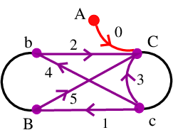
The purple edges left after the construction path in Figure 52:

STEP 2: PURIFIED CONSTRUCTION COMPOSITION
Choose a potential construction path in (a good choice would be one of minimal length among all potential construction paths transversing the maximum number of edges of ). Let be the corresponding purified construction composition, if it exists, as in Lemma 7.22. If the corresponding construction composition does not exist (for example, if one of the is not birecurrent), then try other potential construction paths until one exists with a corresponding construction composition. If none can be found, then one can use Method I to find and determine whether exists at all.
We denote the decomposition of by
and the corresponding sequence of LTT structures by
Example 12.24.
Purified construction composition corresponding to the potential composition construction path in Figure 52:

It should be noted that all relevant LTT structures are Type (*) admissible LTT structures for (and are birecurrent, in particular).
STEP 3: SWITCH
In this step we determine the switch that will precede in the decomposition of . To determine choices that may give the switch, one has to look at the source LTT structure for the first generator in the purified construction composition. There is one potential switch for each purple edge of such that in . Disregard potential switches with source LTT structures that are not birecurrent (or are for other reasons not admissible Type (*) LTT structures). Choose one of the remaining switches and call it . Denote the source LTT structure by .
Example 12.25.
The two options for the switch proceeding the pure construction composition of Example 12.24 can be summed up giving their source LTT structures (as the generator is determined to be by the red edge in . The two source LTT structures are (the black edges in the LTT structures are left out, as they are easily ascertained):

Both of the LTT structures are admissible Type (*) LTT structures, so are options.
STEP 4: RECURSIVE CONSTRUCTION COMPOSITION BUILDING
In order to track our progress in ensuring that all edges of are actually in the ideal Whitehead graph for we establish the notion of a “preimage subgraph.”
Definition 12.26.
Let (, , ) be a switch. Recall that there exists an isomorphism from to that sends the vertex labeled to the vertex labeled and fixes the second index of the label of all other vertices of (it sends the vertex labeled in to the vertex labeled in for all ). The isomorphism extends naturally from the vertices to the edges.
The preimage subgraph under (, , ) for a subgraph will be denoted and is obtained from by replacing each edge of with its preimage under the isomorphism. In other words, for each edge in there is an edge in and for each edge in , where and , there is an edge in .
Remark 12.27.
One could obtain the preimage subgraph from simply by changing the label in of to , as well as the labels to for .
We define here further notation that will also be used to track our progress in ensuring that all edges of are actually in the ideal Whitehead graph for .
Definition 12.28.
For the purified construction composition with destination LTT structure we define as the subgraph of consisting of precisely the purple edges in the construction path for . Let denoted the set of purple edges in the construction path for . Then and we inductively define as .
Now that we have established the notation to do so, we describe the recursive process of construction composition building.
Recursive Process:
The following steps are repeated recursively until for some .
- I.
-
Determine the first building subgraph for .
- II.
-
Find a potential construction path in (an “optimal strategy,” similar to that in Step 2, may involve choosing the path to be of minimal length among all potential construction paths transversing the maximum number of colored edges of ). Let be the corresponding purified construction composition, if it exists, as in Lemma 7.22. If the corresponding construction composition does not exist (for example, if one of the in the decomposition is not birecurrent), then try other potential construction paths until one has a valid corresponding construction composition. If no valid corresponding construction composition can be found, then try using different construction compositions in the previous steps. If this does not work, one can use Method I to find and determine whether exists at all.
We denote the decomposition of by
and the corresponding sequence of LTT structures by
- III.
-
Determine : There is one potential switch for each purple edge of such that in . Disregard potential switches with source LTT structures that are not birecurrent (or are for other reasons not admissible Type (*) LTT structures). Choose one of the remaining switches and call it . Denote the source LTT structure for by .
- IV.
-
Repeat (I)-(III) recursively until for some .
Example 12.29.
We continue with the example for Graph XIII
![[Uncaptioned image]](1205.5320v1/Example5.1Page2New2.png)
![[Uncaptioned image]](1205.5320v1/Example5.1Page2New2.5.png)
![[Uncaptioned image]](1205.5320v1/Example5.1Page3New2.png)
STEP 5: CONCLUDING SWITCH SEQUENCE
Once we have that , we find the shortest possible switch sequence
with as the source LTT structure and as the destination LTT structure. A switch path in may be used for this purpose, though it will be necessary to check that each with is an admissible Type (*) LTT structure for (and, in particular, is birecurrent).
If it is not possible to get a pure sequences of switches, then one can try any permitted composition with as its source LTT structure (and its destination LTT structure) or, if necessary, find a path in from to (see Method I). It may be possible to find the path in without actually building the entire diagram by instead just looking at the portion of the permitted extension/switch web constructed starting with (see Method I).
Example 12.30.
We continue with the example for Graph XIII.

At this point we have the final map and get:

We showed that this map does not have any PNPs in Section 10.
Remark 12.31.
There are choices for the switches at the beginning of each construction composition that make for shorter and simpler representatives. The following guidelines are helpful.
- (1)
We want that the switch changes the unachieved direction to be in a pair that does not contain the unachieved direction for for any .
- (2)
We want to maximize the number of edges of that constructs that have not yet been constructed by the with . To do this it helps that the switch does not result in an unachieved direction pair where a lot of the edges in that are not transversed by the construction path contain the vertex labeled .
STEP 6: FINAL CHECKS
The map is not acceptable if any of the following holds:
- (1)
for some vertex edge pair , neither nor is the red vertex in any LTT structure in the decomposition;
- (2)
there are not fixed directions; or
- (3)
the map constructed has a PNP.
Check (1) visually, check (2) by composing directions maps of the generators, and then check (3) via the procedure in Section 10. If (1) fails, then one can try finding an alternative concluding switch sequence resolving the problem. If (2) fails, one can simply take a power of the map so that all periodic directions are fixed.
12.3 Method III
- (A)
-
Find a switch sequence with such that, for each vertex pair , either or is the red vertex in some LTT structure in the sequence. (Such a composition would be represented by a loop in and can be found as a loop in if not by trial and error. It would also work to use a loop in that does not represent a switch sequence, but the condition on vertex pairs still holds.)
- (B)
-
As in Method II, find a construction path in transversing as many edges of as possible, except that we now have the added condition that the corresponding purified construction composition must start and end with the same LTT structure.
- (C)
-
Proceed as in Method II with the added condition of (B) and with the condition that the switches between the purified construction compositions are determined by the switch sequence .
- (D)
-
The map constructed is not acceptable if it has any PNPs and so the procedure of Section 10 must be used to check that it does not have any PNPs. It is additionally still important that all periodic directions are fixed and that the map constructed has all of as its ideal Whitehead graph. Reference Method II for how to ensure this is the case.
Example 12.32.
We return to Graph XX:
A switch sequence for this graph is given in Example 7.32. Our first construction composition was given in Example 7.24. What was still needed after that composition was:
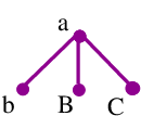
We take the preimage under the direction map for the final switch and get:
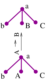
Since we could not obtain all of these edges from a single construction composition, we take another preimage:
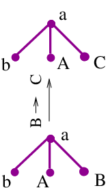
We use the construction composition for the following construction path to obtain these edges:
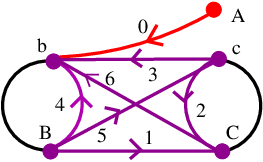
When composed we get:

The automorphism we have obtained is:
The periodic directions for this map are not fixed. However, they are fixed when we compose with itself, so we take .
13 Unachievable Ideal Whitehead Graphs
The unachievability of Graph VII was shown in Section 12. In this section we show that Graph II and Graph V are also unachievable. In all figures of this section, we continue with the convention that X represents , etc.
13.1 Four Edges Sharing a Vertex (Graph II)
The first unachievable 5-vertex Type (*) pIW graph is the graph consisting of four edges adjoined at a single vertex. For this graph we use Proposition 5.4. What we need is that every Type (*) Admissible LTT Structure for is not birecurrent. Up to EPP-isomorphism, there are two such LTT structures to consider neither of which is birecurrent):

These are the only structures worth considering as follows:
Either three of the valence-one vertices of belong to different edge pairs or the valence-one vertices are labeled with two sets of edge pairs. First consider the case where the valence-one vertices are labeled with two sets of edge pairs. The red edge cannot be attached in such a way that it is labeled with an edge pair and all the other resulting LTT structures are the same as the first structure up to EPP-isomorphism. Now consider the case where three of the valence-1 vertices of belong to different edge pairs. One of these three have the label of the inverse of the valence-four vertex. The red edge can only be attached at one vertex choice and without causing an edge pair labeled vertex set connected by a valence-1 edge in the colored subgraph of the LTT structure. Up to EPP-isomorphism, this just leaves us with the second structure.
13.2 Graph V
We draw the illustrative AM diagram here without labels on the edges because it is clear even from this much that no map represented by a loop in this diagram would be irreducible (the only edge pairs labeling red vertices are and ):

14 Achievable 5-Vertex Type (*) pIW Ideal Whitehead Graphs in Rank 3
This section includes the main theorem of this document. For the theorem we use our methods to determine which -vertex Type (*) pIW graphs arise as for ageometric, fully irreducible . Since there are precisely twenty-one -vertex Type (*) pIW graphs (see Figure 1 for a complete list), we can handle them on a case-by-case basis. For all figures of this section we continue with the convention that A notates .
Theorem 14.1.
Precisely eighteen of the twenty-one 5-vertex Type (*) pIW graphs are ideal Whitehead graphs for ageometric, fully irreducible .
Proof: The unachievable graphs (Graph II, Graph V, and Graph VII) were already handled in sections 12 and 13. We now give representatives for the remaining graphs, leaving it to the reader to prove that these representatives are PNP-free (using the procedure of Section 10), have Perron-Frobenius transition matrices, and have the appropriate ideal Whitehead graph. Proposition 11.4 then gives that they are representatives of ageometric, fully irreducible with the desired ideal Whitehead graphs.
GRAPH I (The Line):
We give here the representative whose ideal whitehead graph, , is GRAPH I:
Our ideal decomposition for is described by the following figure:
For this we constructed a component of and used Method I. This method made the most sense here as there were only a few birecurrent LTT structures to be included in .
GRAPH II:
The representative whose ideal whitehead graph, , is GRAPH II was again constructed using Method I. We started with a path in .

The path in corresponds to the ideal decomposition:
![[Uncaptioned image]](1205.5320v1/Example1.5.png)
And our representative is:
GRAPH IV:
The representative whose ideal whitehead graph, , is GRAPH IV is:
We used Method I here. Constructing was exceptionally easy because of the symmetry in the graph. Our ideal decomposition for is:
![[Uncaptioned image]](1205.5320v1/Example3New.png)
GRAPH VI:
The representative whose ideal whitehead graph is GRAPH VI is:
Our ideal decomposition for is described by the following figure:
![[Uncaptioned image]](1205.5320v1/Example19.png)
GRAPH VIII:
The representative whose ideal whitehead graph, , is GRAPH VIII is:
Our ideal decomposition for is described by the following figure:
![[Uncaptioned image]](1205.5320v1/Example13.png)
For this we constructed a component of and used Method I. This method made the most sense here as there were only a few birecurrent LTT structures to be included in .
GRAPH IX:
The representative whose ideal whitehead graph, , is GRAPH IX is:
Our ideal decomposition for is described by the following figure:
![[Uncaptioned image]](1205.5320v1/Example14.png)
GRAPH X:
The representative whose ideal whitehead graph, , is GRAPH X is:
Instead of giving our entire ideal decomposition here, we give a condensed decomposition where construction compositions starting and ending at a graph are shown as paths below it. This is an example of a case where Method III is used to find our desired representative. If you leave out the initial generator (the upper left-most) and the pure construction compositions corresponding to the paths indicated, we have a switch sequence.
![[Uncaptioned image]](1205.5320v1/Example10New.png)
GRAPH XI:
The representative whose ideal whitehead graph, , is GRAPH XI is:
Again, instead of giving our entire ideal decomposition here, we give a condensed decomposition where construction compositions starting and ending at a graph are shown as paths below it. However, the graph in the lower right actually gives a construction composition with source LTT structure above it to the left and destination LTT structure above it to the right. This representative thus actually uses a variant of Method III where we allow this. (We in fact use a combination of Method II and Method III).
![[Uncaptioned image]](1205.5320v1/Example15.png)
GRAPH XII:
The representative whose ideal whitehead graph is GRAPH XII is:
Again, instead of giving our entire ideal decomposition here, we give a condensed decomposition where construction compositions starting and ending at a graph are shown as paths below it.
![[Uncaptioned image]](1205.5320v1/Example17.png)
GRAPH XIII:
The representative whose ideal whitehead graph is GRAPH XIII is:
Our ideal decomposition for this representative and further explanation were given in Example 12.29.
GRAPH XIV:
The representative whose ideal whitehead graph is GRAPH XIV is:
Our ideal decomposition for is described by the following figure:
![[Uncaptioned image]](1205.5320v1/Example11.png)
GRAPH XV:
The representative whose ideal whitehead graph, , is GRAPH XV is:
Again, instead of giving our entire ideal decomposition here, we give a condensed decomposition where construction compositions starting and ending at a graph are shown as paths below it. The similarities between this construction and that of Graph XI are not a coincidence. Since XI is a subgraph of XV missing only a single edge, once the representative for XI was constructed, we could alter the representative by adding the edge [] to the final (right-most) construction path to add that edge to . It must also be checked, however, that, if we add the preimages of this edge into the previous LTT structures that they are still birecurrent, that we still have a composition of switches and extensions, that we still have no PNPs, and that our initial and terminal LTT structures for the entire train track are the same.
![[Uncaptioned image]](1205.5320v1/Example16.png)
GRAPH XVI:
The representative whose ideal whitehead graph is GRAPH XVI is:
Our ideal decomposition for is described by the following figure:
![[Uncaptioned image]](1205.5320v1/Example6NewNew.png)
GRAPH XVII:
The representative whose ideal whitehead graph is GRAPH XVII is:
Our ideal decomposition for is described by the following figure:
![[Uncaptioned image]](1205.5320v1/Example18.png)
GRAPH XVIII:
The representative whose ideal whitehead graph is GRAPH XVIII is:
Our ideal decomposition for is described by the following figure:
![[Uncaptioned image]](1205.5320v1/Example4RevisedNew.png)
GRAPH XIX:
The representative whose ideal whitehead graph is GRAPH XIX is:
Again, instead of giving our entire ideal decomposition here, we give a condensed decomposition where construction compositions starting and ending at a graph are shown as paths below.
![[Uncaptioned image]](1205.5320v1/Example12New.png)
GRAPH XX:
The representative having ideal Whitehead graph GRAPH XX, where
was constructed in the examples above.
GRAPH XXI (Complete Graph):
The representative whose ideal whitehead graph is GRAPH XXI is:
Below we include an ideal decomposition of the representative. We only label the vertices of the red edge in each graph of this example since the remainder of the graph is completely symmetric and so any permutation of the remaining labels gives exactly the same graph. This is an example of a case where Method I would have been extremely impractical and Method II was particularly easy to apply. Similar methods as used to construct this representative could also be used to construct the representative whose ideal Whitehead graph is the complete graph in any odd rank greater than five.
![[Uncaptioned image]](1205.5320v1/Example7_CompleteGraph.png)
Since we have either given representatives yielding or shown that they cannot exist for all twenty-one Type (*) pIW graphs with five vertices, we have completed the proof.
QED.
References
[BF94] M. Bestvina, M. Feighn, M. Handel, Outer Limits, preprint, 1993; available at
http://andromeda.rutgers.edu/ feighn/papers/outer.pdf.
[BFH00] M. Bestvina, M. Feighn, M. Handel, The Tits alternative for I: Dynamics of exponentially-growing automorphisms, Ann. Math. 151 (2000), 517-623.
[BFH97] M. Bestvina, M. Feighn, M. Handel, Laminations, trees, and irreducible automorphisms of free groups, Geom. Funct. Anal. 7 (1997), 215-244.
[BFH97] M. Bestvina, M. Feighn, M. Handel, Erratum to: Laminations, trees, and irreducible automorphisms of free groups, Geom. Funct. Anal. 7 (1997),1143.
[BH92] M. Bestvina, M. Handel, Train tracks and automorphisms of free groups, Ann. Math. 135 (1992), 1-51.
[CP10] M. Clay, A. Pettet, Twisting Out Fully Irreducible Automorphisms, Geom. Funct. Anal. 20 (2010), no. 3, 657-689.
[CV86] M. Culler and K. Vogtmann, Moduli of Graphs and automorphisms of free groups, Invent. Math. 84 (1986), 91-119.
[CP84] D. Cvetkovic , M. Petric , A table of connected graphs on six vertices, Discrete Math. 50 (1984) 37 49.
[FB86] Farb, Benson and Margalit, Dan. A Primer on Mapping Class Groups, Princeton: Princeton University Press, 2012.
[GJLL98] D. Gaboriau, A. Jaeger, G. Levitt, and M. Lustig, An Index for counting fixed points of automorphisms of free groups, Duke Math. J. 93 (1998), no. 3, 425-452.
[HM11] M. Handel and L. Mosher, Axes in outer space, American Mathematical Society, 2011.
[LL03] Levitt, Gilbert; Lustig, Martin, Irreducible automorphisms of Fn have north-south dynamics on compactified outer space. J. Inst. Math. Jussieu 2 (2003), no. 1, 5972.
[MS93] H. Masur and J. Smillie, Quadratic differentials with prescribed singularities and pseudo-Anosov diffeomorphisms, Comment. Math. Helv. 68 (1993), no.2, 289-307.
[P88] R.C. Penner. A construction of pseudo-Anosov homeomorphisms, Trans. Amer. Math. Soc., 310 (1988) No 1, 179-197.
[N86] Jakob Nielsen: collected mathematical papers. Vol. 1. Edited and with a preface by Vagn Lundsgaard Hansen. Contemporary Mathematicians. Birkhäuser Boston, Inc., Boston, MA, 1986. xii + 459 pp.
[St83] J. R. Stallings, Topology of Finite Graphs, Inv. Math. 71 (1983), 552-565.
[W36] J. H. C. Whitehead, On certain sets of elements in a free group, Proc. London Math. Soc., 41 (1936), pp. 4856.