New parton distributions in fixed flavour factorization scheme from recent deep-inelastic-scattering data
Abstract
We present our QCD analysis of the proton structure function to determine the parton distributions at the next-to-leading order (NLO). The heavy quark contributions to , with = , have been included in the framework of the ‘fixed flavour number scheme’ (FFNS). The results obtained in the FFNS are compared with available results such as the general-mass variable-flavour-number scheme (GM-VFNS) and other techniques used in global QCD fits of parton distribution functions. In the present QCD analysis, we use a wide range of the inclusive neutral-current deep-inelastic-scattering (NC DIS) data, including the most recent data for charm , bottom , longitudinal structure functions and also the reduced DIS cross sections from HERA experiments. The most recent HERMES data for proton and deuteron structure functions are also added. We take into account ZEUS neutral current DIS inclusive jet cross section data from HERA together with the recent Tevatron Run-II inclusive jet cross section data from CDF and DØ. The impact of these recent DIS data on the PDFs extracted from the global fits are studied. We present two families of PDFs, KKT12 and KKT12C, without and with HERA ‘combined’ data sets on DIS. We find these are in good agreement with the available theoretical models.
Keywords:
NLO computation, parton distribution functions, heavy quark contributions, fixed flavour number scheme (FFNS).pacs
13.60.Hb, 12.39.-x, 14.65.BtI Introduction
Lepton nucleon deep inelastic scattering (DIS) processes play a very important role for our understanding of quantum chromodynamics (QCD) and nucleon structure [1]. The DIS process of leptons off nucleons is an instrumental tool for high precision measurements of the quark and gluon content of the nucleons. DIS experiments provide valuable information from lepton-nucleon scattering cross sections to find out about the structure functions of targets. Note that these structure functions are related to parton distribution functions (PDFs) directly. This process at large momentum transfer provides one of the cleanest possibilities to test the predictions of QCD and allows us to measure the high-precision PDFs of the nucleons together with the strong coupling constant. DIS process also demonstrates the internal structure of the nucleon in high-energy scattering at the CERN Large Hadron Collider, Fermilab Tevatron collider, and in other hard scattering experiments. The advent and development of the electron-proton colliders, especially HERA, has resulted in significant progress in the recent years on the precise understanding of the structure of the nucleon, especially in different kinematic regions of momentum fractions of proton carried by the struck parton. The most precise inclusive structure function measurements which has been provided by HERA collider, has brought remarkable improvements to our understanding on proton structure and can be used to extract high precision PDFs, which is important for any process which involves colliding hadrons.
Recently it is quite common for several theoretical groups to make a global fit on available experimental data to extract parton distribution functions which are utterly useful in colliding hadrons, specially LHC, studies. Nowadays thousands of published data points from various experiments are available to extract more precise PDFs and strong coupling constants in higher perturbative orders. Also for more accuracy, the QCD fits can be performed with leading-order (LO), next-to-leading order (NLO) and even next-to-next-to-leading order (NNLO) QCD approximation. In addition, it is also significant to find out about PDFs uncertainties for experimentalist.
In recent years, a number of theoretical groups providing global QCD fits (CTEQ/CT10 [2, 3] and MRST/MSTW08 [4, 5, 6]) have developed a prescription for determining uncertainties, and have now been joined by several other theoretical groups (NNPDF [7, 8, 9], ABKM10 [10], GJR08/JR09 [11, 12]). HERA experimental collaborations have combined their DIS data and published parton distribution functions, (HERAPDF), with uncertainty error bands as well [14, 13].
Nowadays, new PDFs incessantly become more accurate by considering up-to-date theoretical developments and data from hadron colliders experiments, also such evolvement provide more reliable calculation of uncertainties corresponding to different theoretical and experimental inputs. The correct treatment of heavy quark flavours in global QCD analysis of PDFs is essential for precision measurements at hadron colliders such as HERA, since it contributes up to 30% to the DIS inclusive cross section at small . This is very important for the reliability of parton distributions in the kinematic region corresponding to the foreseen experiments at LHC since DIS remains an incomparable source of information about parton distributions at small , despite the effect of collider data on the PDFs. Recent reported results [15, 16, 17, 5, 18, 19, 20, 21] show that the cross section of Higgs, W and Z production at the LHC are sensitive to detailed aspects of PDFs that depend on the heavy quark mass effects; and standard model processes as well as beyond standard models considerably depend on improved knowledge of the c-quark parton density, in addition to the light flavours density [22]. Heavy quark flavours production in DIS is calculable in QCD and provides significant information on the gluonic content of the proton. Nowadays, heavy quarks are produced in several experiments of high energy physics and the production and decay properties of the heavy quarks are extremely interesting. A number of theoretical groups, such as CTEQ collaboration, CT10 [3], MSTW08 [6], ABKM10 [10] and GJR08 [11] have produced publicly available PDFs using different data sets. We also studied the diffractive process to parameterize the diffractive parton distribution functions (DPDFs) taking into account heavy quarks contributions using recent experimental data [23].
In the present paper we will extract the PDFs using QCD analysis of a large number of available and up-to-date experimental data in the frame work of FFNS by introducing a new kind of parametrization. This paper deals with the construction of a FFNS and the comparison of their predictions with the most recent experimental data for various region of and . Since we have recent experimental data for the reduced cross section, heavy quarks and longitudinal structure functions from the HERA collaboration, and new fixed target data for proton and deuteron structure functions from HERMES, we have enough motivation to extract all of parton distribution functions using new sets of parametrization with take into account the heavy quark contributions.
The organization of the paper is as follows. In Sec. II, we outline the theoretical formalism which describes the DIS structure functions. Our parametrization and heavy quark contributions to the proton structure function and the formulation of FFN scheme are also performed in this Section. In Sec. III, we discuss the global parton analysis and then present the results of our NLO PDF fit to the DIS world data to determine the PDF parameters and . Discussion of fit results are given in Sec. IV. This section also contains a detailed comparison of the KKT12 and KKT12C QCD fits with other recent PDF sets and with the recent HERA data in various and regions. The results related to the longitudinal structure function is presented in Sec. V. Section VII contains our summary and conclusions.
II Theoretical background of the QCD analysis
In this section, we first give a brief overview of the standard theoretical formalism that we used in the present QCD analysis. A more detailed description is given later in separate sections.
II.1 Theoretical input
The QCD predictions for the structure functions are obtained by solving the well known DGLAP evolution equations at NLO in the modified minimal subtraction () scheme. We choose the factorization and renormalization scales to be . We work in the scheme, where the deep-inelastic nucleon structure function , can be written as a convolution of the parton distribution functions together the coefficient functions [6]. The scale dependence of the PDFs is given by the well-known DGLAP evolution equations which yield the PDFs at all values of if they are provided as functions of at the input scale of .
A number of methods to solve the evolution equations have been proposed, including direct -space method, Mellin-transform methods and orthogonal polynomials methods. More detailed about the later method are given in Refs. [24, 25, 26, 27, 28, 29, 30, 31, 32, 33, 34, 35].
In the present paper we have performed all Q2-evolutions in Mellin -moment space for the NLO evolution. In this regard, the program QCD-PEGASUS [36] is used in order to perform all Q2-evolutions of parton distributions. The input for the evolution equations and the strong coupling constant , at a reference input scale taken to be Q = 2 GeV2, must be extracted from a global QCD analysis of DIS world data.
Our present standard NLO QCD analysis has been performed within the factorization and renormalization scheme. We do not consider the heavy quarks (, , ) as massless partons within the nucleon. In this case, the number of active (light) flavours appearing in the Wilson coefficients and the corresponding splitting functions to be fix at . Furthermore, the evaluation of the running strong coupling needs to match at , i.e. .
II.2 Parametrization
For the QCD fit in the present analysis we use the following independent functional form of the parametrization of the parton distribution functions at the input scale =2 GeV2 for the valence quark distributions and , the anti-quark distributions , , and for gluon distribution :
| (1) |
The flavour structure of the light quark sea at is taken to be
| (2) | |||||
| (3) | |||||
| (4) |
and we take a symmetric strange sea due to the insensitivity of data sets we are using to the specific choice of the strange quark distributions. Due to the very large amount of data in our global QCD fits and the presence of some constrains, we can control the parameters in order to allow sufficient flexibility in the form of the parton distributions.
In the present work, the input PDFs listed in Eq. 1 are subject to three constraints from valence quarks number sum rules together with the total momentum sum rule [6]. Not all the parameters in our inputs for the parton distributions are free. The parameters , and were calculated from the other parameters using mentioned constrains, therefore there are potentially 28 free parameters in the PDF fit, including .
The mentioned parametrization for the input PDFs in our analysis, Eq. 1, and all free PDF parameters listed there allow the fits a large degree of flexibility. In the final minimization, we fixed some parameters and only 13 parameters remained free for all parton flavour in the fits. These parameters are allowed to go free in order to calculate the covariance matrix.
According to our parameterization in Eq. 1 and for valence quark distributions, and , we use the standard functional form. The normalization parameter is obtained from the number of valence quarks sum rules. The variation of the valence distributions at intermediate values of will be controlled by the third free parameter . In our calculation for valence sector, we found that the parameter is correlated to and more strongly. At very high and even at very small , the uncertainties are constrained by the mentioned sum rules. In the region of =[0.01, 0.75], where the valence PDFs are constrained by DIS data, about 75% of the total number of valence quarks can be found. We should notice that in the reported results of MSTW08 [6] and GJR08 [11] for input parametrization, the parameter value of is fixed to 0.5 which we want to deal with this parameter as a free parameter. After first minimization, in both cases of valence quark distributions, we will get the parameter values of , and fixed so only two parameters remain free, and .
In order to consider the flavour separation of the sea-quark distributions in Eq. 1, we choose as a power of for , because at high this PDF is becoming very small and we attempt to constrain and to be positive. We need also to have term instead of the more usual and term to give sufficient flexibility at medium and large . In fact we consider , and as free parameters and , and will be fixed at their best-fit values.
In the sea quark distribution, in Eq. 1, there is no sum rule constraint, so in principle there are 3 free parameters including , and and the other 3 parameters will expected to be fixed since the data do not constrain these parameters well enough.
The gluon distribution is a far more difficult case for PDFs parameterizations to obtain precise information. Since the current data provide little constraint on the gluon density, we expect the functional form of gluon distributions in Eq. 1 to allow us for better gluon PDF determination. The input gluon in the MSTW08 [6] is almost the same form of the original MRST fits [37, 38], but MSTW08 added a second term to avoid a negative gluon distribution at very small . We found that the parameter in our gluon parametrization could help us to facilitate this. In this case we need to have a term instead of the more usual term to give sufficient flexibility at low , and we find stability in the QCD fits. On the other hand, one feature of our parametrization is that we allow the gluon to have a very general form over a wide range of , specially at medium , because it can induce potentially large effects on the strong coupling constant obtained from the global fits and indirectly leads to a change in the light partons. In particular, fixing the parameters , and at the best fit values we find that and are sufficient for the gluon – one for high and one for low . Consequently in the final minimization, only two parameters and remain free. We note that we can determine by the total momentum sum rule [6].
As a last point, we note that the single-inclusive jet data are very important for the constrains of gluon distribution. The constraints on the gluon distributions in the domain are provided by the inclusive jet production data from Run II at the Tevatron from CDF and DØ while the data from HERA on inclusive jet production in DIS constrain the gluon for .
II.3 Treatment of heavy flavours
In this section, we will discuss the fixed flavour number (FFN) scheme parton model predictions at high energy colliders at LO and NLO of QCD. It is expected that perturbative QCD at NLO should give a good description of heavy quark flavour production in hard scattering processes, so the correct treatment of heavy flavours in common QCD analysis of PDFs at this order is essential for precision measurements at hadron colliders. The LO and NLO heavy quark contributions to the proton structure function are calculated in the FFN approach and contribute to the total structure functions as where the refers to the common (anti) quarks and gluon initiated contributions, and with . Charm and bottom quark contributions to the total DIS cross section at high are up to 30% and 3%, respectively, and top quark contributions are negligible at present energies. As already mentioned at the end of Sec. II.1, we employ for our analysis the FFN scheme and fix the number of active light flavours = 3 in all splitting functions and in the corresponding Wilson coefficients. In this factorization scheme only the light quarks (, , ) are genuine, i.e., massless partons within the nucleon, whereas the heavy ones (, , ) are not.
Fixed flavour number approach is the region where the hard scale of the DIS process is around the quark mass, i.e. where . In this case, massive quarks are not considered as partons within the proton. They are described as final-state particles and so they are entirely created in the final-state. Our practical reason for extracting partons from the fits to structure function data in the fixed three-light-flavour () is to have a set of up-to-date partons in order to make consistent comparisons between other parton sets available using the same theoretical framework of other scheme such as general mass variable-flavour number scheme (GM-VFNS) [3, 6] and FFNS [11]. In addition for many exclusive or semi-inclusive processes the theoretical predictions for the hard scattering cross sections are only available in the FFN scheme. The different heavy quarks treatment which nearly every group does, may led to different results for the extracted parton distribution functions.
II.4 Fixed flavour number scheme (FFNS) and structure function
The NLO QCD analysis presented in this paper is performed in the modified minimal subtraction () factorization and renormalization scheme. Heavy quarks (, , ) are not considered as massless partons within the nucleon and all their effects are contained in the perturbative coefficient functions. This defines the so-called “fixed flavour number scheme” (FFNS), which is fully predictive in the heavy quark sector and incorporates the correct threshold behavior. In the common factorization scheme, the relevant total proton structure function as extracted from the DIS process can be, up to NLO, written as [6, 10, 11, 12, 39, 40, 41]
| (5) | |||||
with the non–singlet contribution for three active (light) flavours are given by
| (6) | |||||
where and is the common NLO coefficient function [42, 43, 44] . The NLO -evolution of the flavour non–singlet combinations and is related to the LO (1-loop) and NLO (2-loop) splitting functions and respectively [42, 43] .
The flavour singlet contribution in Eq. 5 reads
| (7) | |||||
with , and the additional NLO gluonic coefficient function can be found in Refs. [42, 44] for example. Notice that we consider sea breaking effects () since the HERA data is used, and thus our analysis are sensitive to these corrections. Since these data sets are also insensitive to the specific choice of the strange quark distributions, we consider a symmetric strange sea, . We also use where in practice is a constant fixed to . The heavy flavour contributions that have been added in the present analysis will be discussed in the next section.
II.5 Heavy flavour contributions
The heavy flavour contributions which have been added in the present analysis are taken as in Refs. [41, 45, 46, 47, 48, 49, 50] . The structure functions in fixed flavour factorization scheme are written by
| (8) |
where represents only to the light partons ( = , , …), refers to the mass of the heavy quarks, with = , and denotes the number of active flavour.
The FFNS approach which we are using in the present analysis, contains all the heavy quark mass dependent contributions. In leading order of QCD, , the well known FFN scheme heavy quark flavour contributions in collisions are dominated by the photon gluon fusion process (BGF), [51, 52, 53, 54, 55]. The FFNS heavy flavour coefficient functions for neutral-current structure functions containing terms are well known up to NLO. Due to the complexity of the heavy flavour coefficients function caused by the non-zero mass of heavy quarks, , there are no published complete analytic expressions for all the coefficient functions and the results are available in table form at this order [49]. In particular we use the code provided in Ref. [49], which combines known analytic expressions together with grids for the more complicated coefficient functions; they are represented in the factorization scheme. Up to , the relevant heavy quark contributions to DIS structure functions are given by [49, 50]
| (9) |
where the upper boundary on the integration is given by and sum runs over all the light quark and antiquark flavours. Furthermore, denote the light parton densities in the proton and stands for the mass factorization scale, which normally has been put equal to the renormalization scale. is the charge of the heavy quarks, with . The coefficient functions, represented by and by , are calculated in [50] and they are represented in the scheme. The LO contributions to , due to the subprocess with , have been summarized in [55], and the NLO ones are given in [49, 50].
Different groups use various values for the charm and bottom quark masses varying from 1.3 GeV to 1.65 GeV and from 4.3 GeV to 5 GeV, respectively. This variation will change the extracted parton distribution functions. A detailed discussion on mass dependence of parton distribution functions can be found in [5, 9, 56, 57].
In the present analysis we fix the heavy quark masses at and , this differs from the MRST and MSTW08 default values of GeV, GeV and GeV, GeV, respectively. The results of Ref. [6] indicated that if we allow the mass of charm quark as a free parameter in the global fits, one can find the best-fit value to be GeV at NLO.
III Global parton analyses
III.1 Overview of data sets
PDFs are usually determined in a global QCD analyses of a wide variety of DIS data, both from HERA and fixed-target experiments as well as data from CHORUS, NuTeV and data for the longitudinal structure function, . In the recent years, several new precise data sets became available which we include in our present global QCD fit. In the present analysis we fit to the measured neutral current deep inelastic scattering cross section values that is defined by three structure functions, , and as [1, 11]
| (10) |
where is the process inelasticity and is the centre-of-mass energy and .
| Experiment | –range | –range [GeV2] | # of data points | ||
| H1 high Q2 94–97 NC | 0.003 – 0.65 | 150.0 – 30000.0 | 130 [58] | 1.5% | 0.9991 |
| H1 high Q2 98–99 NC | 0.0032 – 0.65 | 150.0 – 30000.0 | 126 [59] | 1.8% | 0.9999 |
| H1 Q2 96–97 NC | 5.0E-5 – 0.2 | 2.0 – 150.0 | 144 [60] | 1.7% | 1.0078 |
| H1 high Q2 99–00 NC | 0.002 – 0.65 | 100.0 – 30000.0 | 147 [61] | 1.5% | 0.9999 |
| H1 Q2 99–00 NC | 5.0E-6 – 0.02 | 2.0 – 12.0 | 85 [62] | 0.5% | 0.9994 |
| H1 Q2 00 NC | 2.0E-4 – 0.1 | 12.0 – 150.0 | 99 [63] | 0.5% | 0.9987 |
| ZEUS SVX 95 NC | 5.4E-5 – 0.0019 | 2.50 – 17.0 | 30 [64] | 1.5% | 1 |
| ZEUS 96–97 NC | 6.32E-5 – 0.65 | 2.70 – 30000.0 | 242 [65] | 2% | 0.9995 |
| ZEUS 06–07 NC | 5.0 E-4 – 0.007 | 20.0 – 130.0 | 162 [66] | 2.7% | 1.0012 |
| ZEUS 98–99 NC | 0.050 – 0.65 | 200.0 – 30000.0 | 92 [67] | 1.8% | 0.9996 |
| ZEUS 99–00 NC | 0.050 – 0.65 | 200.0 – 30000.0 | 90 [68] | 2.5% | 0.9968 |
| H1 03–07 NC | 2.9E-5 – 0.01 | 2.0 – 120.0 | 134 [69] | 4 % | 0.9997 |
| NMC | 0.0045 – 0.5 | 2.50 – 65.0 | 126 [70] | 2 % | 1.0023 |
| NMC | 0.0045 – 0.5 | 2.50 – 65.0 | 126 [70] | 2 % | 1.0023 |
| NMC | 0.008 – 0.675 | 2.23 – 99.03 | 156 [76] | 0.15% | 1 |
| BCDMS | 0.07 – 0.75 | 7.5 – 230.0 | 167 [71] | 3% | 0.9900 |
| BCDMS | 0.07 – 0.75 | 8.75 – 230.0 | 155 [75] | 3% | 0.9900 |
| E665 | 0.0037 – 0.38726 | 2.046 – 64.269 | 53 [72] | 1.85% | 1.0012 |
| E665 | 0.0037 – 0.38726 | 2.046 – 64.269 | 53 [72] | 1.85% | 1.0012 |
| SLAC | 0.007 – 0.65 | 2.01 – 22.21 | 53 [73] | 2% | 1.0128 |
| HERMES | 0.006 – 0.66 | 2.0 – 12.0 | 39 [74] | 7.55% | 1.0167 |
| HERMES | 0.006 – 0.66 | 2.0 – 12.0 | 39 [74] | 7.55% | 1.0167 |
| H1 | 1.3E-4 – 0.02 | 6.50 – 60.0 | 25 [77] | 7.5% | 1 |
| H1 | 0.005 – 0.032 | 200.0 – 650.0 | 4 [78] | 1.5% | 1 |
| H1 | 2.0E-4 – 0.05 | 5.0 – 2000.0 | 29 [79] | 1.5% | 1 |
| H1 | 1.97E-4 – 0.05 | 12.0 – 60.0 | 6 [80] | 1.5% | 1 |
| H1 | 1.3E-4 – 0.00316 | 3.50 – 60.0 | 10 [81] | 1.5% | 1 |
| H1 | 8.0E-4 – 0.008 | 12.0 – 45.0 | 9 [82] | 1.5% | 1 |
| ZEUS | 1.3E-4 – 0.00676 | 4.20 – 111.8 | 5 [83] | 1.8% | 1 |
| ZEUS | 1.3E-4– 0.02 | 4.0 – 130.0 | 18 [84] | 1.65% | 1 |
| ZEUS | 3.0E-5 – 0.03 | 2.0 – 500.0 | 31 [85] | 2.2% | 1 |
| ZEUS | 8.0E-5 – 0.03 | 30.0 – 1000.0 | 8 [88] | 1.5% | 1 |
| H1 | 0.005 – 0.032 | 200.0 – 650.0 | 4 [78] | 1.5% | 1 |
| H1 | 2.0E-4 – 0.05 | 5.0 – 2000.0 | 12 [79] | 1.5% | 1 |
| H1 | 1.97E-4 – 0.05 | 12.0 – 60.0 | 6 [80] | 1.5% | 1 |
| ZEUS | 2.0E-4 – 0.013 | 12.0 – 600.0 | 9 [86] | 2 % | 1 |
| ZEUS | 1.3E-4 – 0.013 | 3.0 – 450.0 | 11 [87] | 2 % | 1 |
| ZEUS | 8.0E-5 – 0.03 | 30.0 – 1000.0 | 8 [88] | 1.5% | 1 |
| H1 | 8.0E-4 – 0.008 | 12.0 – 45.0 | 9 [82] | 1.5% | 1 |
| FNAL E866/NuSea | 0.026 – 0.315 | 54 (Fixed) | 30 [89, 90] | 0.6% | 1 |
| H1/ZEUS | 4.27E-5 – 0.0049 | 2.0 – 110.0 | 127 [60, 66, 69, 91] | - | 1 |
| CHORUS | 0.02 – 0.65 | 2.052 – 81.55 | 50 [92] | 2.1% | 1.0023 |
| NuTeV | 0.015 – 0.75 | 3.162 – 125.89 | 64 [93] | 2.1% | 1.0023 |
| DØ I incl. jets | 90 [99] | 6 % | 1.0021 | ||
| CDF II incl. jets | 76 [100] | 5.8% | 1.0023 | ||
| DØ II incl. jets | 110 [101] | 6.1% | 1.0221 | ||
| ZEUS 96–97 incl. jets | 30 [97] | 2 % | 0.9988 | ||
| ZEUS 98–00 incl. jets | 30 [98] | 2.5% | 0.9980 | ||
| CDF II incl. jets | 20 [102] | 6 % | 0.9972 | ||
| All data sets | 3279 |
Statistically, most significant data that we use in our QCD analysis, which we call “KKT12” fit, are the HERA measurements of the DIS ‘reduced’ cross-section. We use the small and large- from H1 and ZEUS data for GeV2 [58, 59, 60, 61, 62, 63, 64, 65, 66, 67, 68] .
In our QCD fits, we use the most recent H1 and ZEUS combined measurement for inclusive scattering cross sections [14] instead of all the above mentioned data. To distinguish, we call this “KKT12C” when we used the recent H1 and ZEUS combined measurement.
This combined data set contains complete information on DIS cross sections published by the H1 and ZEUS collaborations. The kinematic range of the neutral current data is 0.045 GeV2 30000 GeV2 and 60.65, for values of inelasticity between and . The statistical uncertainty reduces in this measurement.
The most recent HERA structure function data which we use in our analysis are the H1 measurements of the DIS ‘reduced’ cross-section [69]. The kinematic range of the following measurement covers 1.5 GeV120 GeV2 and 2.9. By using these data, we can improve our PDFs, especially at small value.
In addition, we have used the fixed target data of NMC [70], BCDMS [71], E665 [72], SLAC [73] and HERMES [74] all subject to the standard cuts GeV2 and GeV2. Furthermore the fixed target data for [70, 72, 75, 74] and the structure function ratio [76] are both subject to the same standard cuts have been added to the present analysis. These data on , and help us to control the behavior of PDFs in large , which dominated by valence quarks [1].
The H1 and ZEUS measurements on the heavy flavour contribution to structure functions , and of [77, 78, 79, 80, 81, 82, 83, 84, 85, 86, 87, 88] have also been included in the both sets of NLO fits. The Drell–Yan dimuon pair production data of the E866/NuSea (fixed target) experiment [89, 90] have been used.
The direct HERA measurements of the longitudinal structure function, [60, 66, 69, 91] which is a direct constraint on the small region of gluon distribution, have also been included in the present analysis. And finally, we include the data from CHORUS [92] and NuTeV [93] with the same cuts in the present analysis. The importance of data is that the small difference between NC and cross sections data at high Q2, which determines as seen in Eq. 10, contain the valence quark distributions. The reason is that the structure function is related to valence quark contributions and it can provide direct tests of the total valence quark distribution.
We now indicate that we use the deuteron structure function data in our QCD analysis also. Experimental data on the deuteron structure function and the structure function ratio have to be corrected for nuclear shadowing effects [94, 95, 96]. Since the neutron DIS data come from the experiments with nuclear targets such as deuteron, these effects have to be taken into account. Taking the shadowing into account, the deuteron structure function is related in the following way to , and to the shadowing contribution ,
| (11) |
We study the shadowing effect as a nuclear effect in our QCD fits and we found that in the range of 0.10.75 for the NMC, BCDMS and E665 and data, the shadowing effect are very small [96].
The HERA [97, 98] and Tevatron [99, 100, 101, 102, 103] Run I & II data on inclusive jet production in and scattering have been used in our QCD analysis to extract the new sets of parton distribution functions. Take into account the jet production data, constrains the the mid- to high- () gluon density and allows an accurate extraction of strong coupling constant at NLO.
The fastNLO package [104], based on NLOJET++ [105, 106], presents a method that offers an exact and very fast pQCD calculation for a large number of jet data sets. This scenario also allows the inclusion of the NLO hard cross section corrections to both the Tevatron and HERA jet data in the fitting procedure. In the present PDF fits, we use the fastNLO code to take full advantage of direct sensitivity of the jet production data to the gluon density in the proton.
The total data sets that we use in the present global analysis are listed in Table 1 and are ordered according to the type of process. The fitted normalization of the data sets included in the global fit, together with the total normalization uncertainty, , for each data set are also shown in this table. There are 3279 and 2485 data points for KKT12 and KKT12C fits, respectively. We note that the data from Refs. [69] to [93] are used in both of KKT12 and KKT12C QCD fits. It can be a new feature of our analysis that we use a wide range of the most recent DIS data sets including different processes, NC, and scattering to extract all PDFs.
III.2 The method of the minimization and error calculation
III.2.1 Minimization of
The global goodness-of-fit procedure follows the usual chi–squared method with defined as [6, 24, 26, 107]
| (12) | |||||
where denotes the set of independent parameters in the fit, including , and is the number of data points included, (KKT12) and (KKT12C) for the NLO fit. The errors include systematic and statistical uncertainties, being the total experimental error evaluated in quadrature. For the experiment, , , and denote the data value, measurement uncertainty (statistical and systematic combined), and theoretical value for the data point for proton structure function as an example. The theory prediction depends on the input PDF parameters . The KKT12 and KKT12C fits added all uncorrelated and correlated experimental errors in quadrature in the definition. is the experimental normalization uncertainty and is an overall normalization factor for the data of experiment .
In the present analysis, we allow the normalization of several data sets to be free at the same time as the PDF parameters, and then fixed them in the determination of the PDF uncertainties. We also allow a different normalization for each of the HERA running periods. To determine the best fit values at NLO, we minimize the with respect to 27 free input PDF parameters, together with and 23 different data set normalizations, giving a total of 50 free parameters in the fits. The minimization of the above value to determine the best parametrization of the parton distributions is done using the program MINUIT [108]. Due to the limitation of MINUIT package in the practical maximum number of free parameters, we fixed some of the data set normalization to be 1. For example, in the KKT12 fit, we take all the normalization of the H1 and ZEUS data on to be fixed at 1. (See Table 1.) As discussed in Sec. III.1, we use the H1/ZEUS combined data in our KKTC fit, consequently the number of free normalization decreases so we have this chance to allow the data to have different normalization.
III.2.2 Error calculation using Gaussian method
The one errors for the parton density are given by the Gaussian error propagation method as discussed in details in Refs. [109, 110, 111]. In this method, the standard linear errors propagation allows one to calculate the error on any quantity using the formula
| (14) |
where is the allowed variation in and is the covariance, or error matrix of the parameters determined in the QCD analysis at the scale and is the number of free input parameters in the global fit (see Table 2).
| 2.39 | |||||||||||||
| 7.20 | 2.36 | ||||||||||||
| -6.30 | -1.86 | 2.22 | |||||||||||
| -1.68 | -5.30 | 7.11 | 3.01 | ||||||||||
| -6.86 | -2.19 | 2.65 | 8.74 | 6.54 | |||||||||
| -4.51 | -1.40 | 1.38 | 4.33 | -1.21 | 2.38 | ||||||||
| -1.01 | -2.96 | 2.95 | 8.07 | -1.10 | 4.56 | 7.91 | |||||||
| 3.62 | 1.06 | -1.56 | -5.40 | -1.72 | -9.29 | -1.92 | 1.41 | ||||||
| 2.88 | 8.76 | -7.16 | -1.89 | 2.18 | -6.40 | -1.26 | 5.11 | 1.17 | |||||
| 9.96 | 3.16 | -6.12 | 1.60 | 3.98 | -1.72 | -2.89 | -9.68 | 2.53 | 1.85 | ||||
| 6.01 | 1.81 | -1.66 | -4.62 | -2.07 | -1.22 | -2.52 | 9.89 | 6.74 | 2.47 | 1.67 | |||
| 4.23 | 1.33 | -1.09 | -2.72 | -9.46 | -8.13 | -1.77 | 6.13 | 5.88 | 2.18 | 1.16 | 1.07 | ||
| 7.54 | 2.23 | -1.86 | -5.08 | -1.50 | -1.47 | -3.01 | 1.04 | 1.02 | 3.54 | 2.04 | 1.39 | 2.91 |
Consequently one can calculate the error of any quantity by using Hessian or covariance matrix. This method recently used in our nucleon polarized and un-polarized structure function QCD analysis [111, 112, 113]. The covariance matrix elements for 13 parameters in the KKT12 fit are given in Table 2. We able to calculate the uncertainties of PDFs using these covariance matrix elements based on the Gaussian method as mentioned in this section. Their value at are calculated by the QCD evolution.
IV Discussion of fit results
Both KKT12 and KKT12C fits show acceptable agreements with the data sets listed in Table 1. In order to discuss the fit results, we will concentrate on KKT12 fit. Since the outcome of the KKT12 and KKT12C for is almost similar and for PDFs is slightly different, we will show the results of both QCD fits in some figures separately.
IV.1 Detailed comparison to the HERA and fixed target data
Representative comparisons of our results with the relevant HERA (H1 and ZEUS) data [58, 59, 60, 61, 64, 65] on the structure function of the proton, , are presented in Figs. 2 and 2. As shown, the data are well described throughout the whole medium– to small– region for 1.5 GeV2, and thus perturbative QCD is here fully operative. It should be emphasized that the perturbatively stable QCD predictions are in agreement with all recent high statistics measurements of the -dependance of in wide range of .


A detailed comparison of our next-to-leading order (NLO) () results for with a selection of HERA data [58, 59, 60, 61, 64, 65] and fixed target data of NMC [70], BCDMS [71] and SLAC [73] are shown in Fig. 3 To facilitate the graphical presentation we have plotted with indicated in parentheses in the figure.

A comparison of our KKT12C theory predictions for the reduced cross section with the H1/ZEUS combined NC and data [14] are shown in Figs. 4, 5 and 6. The error bars in the figures indicate the total experimental uncertainty. From the figures it is clear that our KKT12C fits are in acceptable agreement with the combined H1/ZEUS set of reduced DIS cross sections.


Fig. 7 shows our prediction for reduced cross section, as a function of and for different value of , in comparison with the most recent data from H1 collaboration [69].

IV.2 KKT12 and KKT12C PDF sets
The resulting parameters of the KKT12 and KKT12C fits are summarized in Table 3. The for both PDFs fits also shown as well. As mentioned in Sec. II.2, the values without errors have been fixed after a first minimization since the data do not constrain these parameters well enough. The parameter errors quoted are due to the propagation of the statistical and systematic errors in the data.
| Parameter | Fit A - (KKT12) | Fit B - (KKT12C) |
|---|---|---|
| 0.3346 | 0.3753 | |
| 0.3271 0.0039 | 0.3126 0.0041 | |
| 3.5858 0.0123 | 3.6536 0.0103 | |
| 0.4573 | 0.5036 | |
| 5.4618 | 3.2716 | |
| 20.1864 | 21.2864 | |
| 0.3730 | 0.6124 | |
| 0.3668 0.0105 | 0.4226 0.0092 | |
| 4.8277 0.1001 | 5.1529 0.0654 | |
| 0.6306 | 0.9553 | |
| 4.6633 | -3.7475 | |
| 7.5520 | 14.1380 | |
| 10.0048 0.8417 | 15.8096 0.3160 | |
| 1.7030 0.0290 | 1.4430 0.0336 | |
| 9.8938 0.3506 | 10.4343 0.4278 | |
| 0.6625 | 0.4972 | |
| -7.3512 | -7.5151 | |
| 23.7067 | 20.4901 | |
| 0.3494 0.0019 | 0.3506 0.0023 | |
| -0.1740 0.0012 | -0.1775 0.0012 | |
| 8.2970 0.0953 | 8.9898 0.0990 | |
| 0.5129 | 0.8764 | |
| 0.2434 | 0.4549 | |
| 9.8585 | 12.4246 | |
| 6.2512 | 7.1383 | |
| 0.1179 0.0101 | 0.1348 0.0051 | |
| 8.4027 0.1663 | 10.0188 0.1494 | |
| 0.2600 | 1.3264 | |
| -1.4998 | -0.9499 | |
| 3590.589/3266 = 1.098 | 2622.118/2472 = 1.060 |
The KKT12 and KKT12C fitted parton distribution functions at NLO for all sets of parametrizations and their errors at the starting scale Q = 2 GeV2 are presented in Figs. 8 and 9. The colored bands show uncertainties on these parton distributions. By having the covariance matrix, it is possible to determine the uncertainties of our PDFs for both fits. Although some of the extracted PDF parameters of two fits are a little different but in total we found no big differences between the best-fit solutions of the two PDF fits. But the error bound for some PDFs of two sets are different.


IV.2.1 Comparison with other recent PDF sets
Our best-fit KKT12 PDFs for -, -, -quark and gluon distributions are shown in Figs. 10 together with a comparison of our results with CT10 [3], MSTW08 [6], ABKM10 [10] and GJR08 [11].

In Fig. 11 the valence quark distributions and are shown as a function of at = 100 GeV2 in the NLO approximation which have been compared with the results obtained by CT10 [3], MSTW08 [6], ABKM10 [10], GJR08 [11] and KT08 [26].

The NLO results for and as a function of in comparison to the results obtained by CT10 [3], MSTW08 [6], ABKM10 [10] and GJR08 [11] have been shown in Fig. 12. The E866/NuSea results [89, 90], scaled to fixed Q2=54 GeV2, are shown as the circles with statistical and systematic uncertainties. The accurate measurements from the E886/NuSea experiments from give clear evidence of the asymmetry as seen in Fig. 12. The asymmetry seems to reach a maximum at , and becomes small at smaller values.

IV.2.2 Impact of the H1/ZEUS Combined data
In order to investigate the effect of H1/ZEUS combined reduced cross section data on the extracted parton distributions functions, we show the ratios of the PDFs, , in the central PDF sets of the KKT11C and KKT11 fits in Figs. 14 and 14 at GeV2 and GeV2, respectively. The inclusive jet data from HERA and Tevatron Run-II are not included. The following results can be found in Refs. [112, 113]. Clearly the effects of the H1/ZEUS combined data sets is on the behavior of gluon and valence quark PDFs at below around as the Fig. 14 shows. The KKT11C gluon distribution at input scale is dominant for small , i.e. while the KKT11 -valance quark PDFs are slightly enhanced at very small , while the -valance quark PDFs degraded at this region.
In this region, the KKT11 , and distributions are very close to the corresponding KKT11C distributions, therefore . In addition the sea-quark (– , – and –quarks) PDFs are slightly similar at small to large region for these two PDF sets.
Fig. 14 shows how these ratios are impacted by the DGLAP evolution to higher energy at GeV2. At small to large , the ratios for all quarks and the features of PDFs are similar to those at GeV2 described above and have been shown in Figures. The same behavior of the - and -valance quark PDFs at GeV2 is repeated for higher scale, GeV2.
The differences observed between the two KKT11C and KKT11 PDFs sets using the H1/ZEUS combined and the separate HERA data sets are very small, except for the gluon PDFs. At higher scales we have as Fig. 14 shows.


The effect of the H1/ZEUS combined reduced cross section data including the inclusive jet data on extracted PDFs from the present QCD analysis have been shown in Figs. 16 and 16. The results presented in these figures includes the jet data from HERA [97, 98] and Tevatron [99, 100, 101, 102, 103]. The differences observed between the results of for KKT12 PDFs to the KKT12C PDFs at the input GeV2 and even at higher scale GeV2, for the , and distributions are very small and they are slightly similar at small to large region.
As Figs. 16 and 16 show, the mentioned data sets effect the gluon and valence quark PDFs at small , i.e. . The KKT12 gluon and -valance quark distributions both for input and higher scale are dominant at very small , while the KKT12 ratio for -valance quark PDFs are slightly decreases at this region.


IV.3 Comparison of charm and bottom structure functions to the HERA data
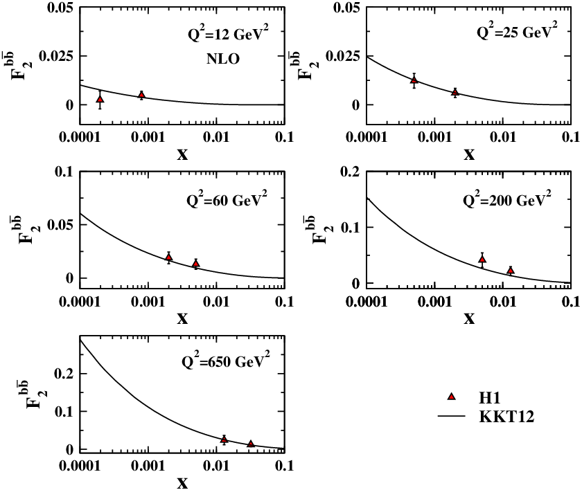
Charm and bottom contributions to the proton structure functions, and , have been extracted from Eq. 9. The detailed discussion of corresponding contributions have been presented in Sec. II.5. The NLO () charm contribution to the proton structure function in the strict of the FFNS with as a function for different values of Q2 and as a function of Q2 for various values are shown in Figs. 17 and 18, respectively. For comparison we also display the charm production data [78, 79, 80, 81, 82, 83, 84, 85] as well.


Fig. 19 shows the NLO () bottom contribution to the proton structure function shown as a function of for various Q2 value in comparison with the charm production data [78, 80]. The structure function ratio as a function of at Q2 = 12, 25, 45 Ge in comparison with H1 data [82] has been shown in Fig. 20.

IV.4 Comparison to the inclusive jet data
As indicated in Sec. III.1, the high- gluon distribution in our global QCD fits is determined by the HERA and Tevatron Run-II inclusive jet data. These data sets have the potential to constrain the gluon density in the proton when used as inputs to global fits of the proton parton distribution functions. In order to illustrate the precision of the KKT12C PDFs, we compare the total cross sections of some selected jet production processes at the Tevatron Run-II from CDF and DØ. Our KKT12C NLO QCD predictions for inclusive jet cross sections are compared to the Tevatron Run-II measurements. Fig. 21 shows the CDF measured inclusive jet cross sections [100], , as a function of in five different regions compared to our KKT12C NLO pQCD predictions. For presentation, the measurements in different regions are scaled by different global factors as indicated in parentheses in the figure. Overall the KKT12C predictions of NLO QCD gives a good description of the data. The DØ Collaboration also reported their measurement of the inclusive jet production cross section [101], in which a comparison was made to our NLO theory calculation (with fastNLO code [104]) based on NLOJET++ [105, 106] using the KKT12C PDF set. The corresponding results of the inclusive jet cross section measurement are displayed in Fig. 22 in six bins as a function of . The comparison shows a good agreement between our NLO theoretical predictions and the data.


V The longitudinal structure function
In this section we turn to the perturbative predictions for longitudinal structure function . Similarly to one can write for in the common factorization scheme for light quark flavour,
| (15) |
Since the longitudinal structure functions contains rather large heavy flavour contributions in the small- region, a consistent analysis has to be taken into account for these effects. The total longitudinal structure function can be written as a sum of where heavy quark contributions are , and the top quark contribution is negligible.

The extracted parton distributions from present analysis have been used to predict . The prediction for the longitudinal structure functions is mainly determined by the form of the gluon distribution extracted from the global QCD analysis. Measuring the structure function therefore provides a way of studying the gluon density and a test of perturbative QCD. The study of , led us to extract heavy quarks, especially gluon distribution function at low .
For completeness, we finally shown our NLO QCD standard predictions for with a representative selection of HERA-H1 data [60, 61, 91, 114] in Fig. 23 and HERA-ZEUS data [66] in Fig. 24 which we used in our QCD analysis.

The predicted longitudinal structure function as a function of has been also compared with the recent H1 data [69] in Fig. 25. Our results for , being gluon dominated in the small- region, are in full agreement with present measurements of .

The longitudinal structure function as a function of and for different values of averaged are shown with the most recent H1 [69] data in Fig. 26. The full error bars in this figure include the statistical and systematic uncertainties added in quadrature. The inner error bars represent statistical error.

VI Determination of the strong coupling constant
The determination of is still an open problem in PDF fits since it’s treatment is closely related to the most important processes at hadron colliders such as the LHC. This importance is due to the dependance of such processes and their partonic cross section to strong coupling constant, . We include as a free parameter in our fits, thus the running coupling constant is determined in our analysis together with the parton distributions of the nucleon; in particular it is closely related to the gluon distribution which drives the QCD evolution. Although some theoretical groups, like CT10 [3] or NNPDF [7, 8], fix the value close to the updated Particle Data Group (PDG) average as [115], but other theoretical groups such as MSTW08 [6], ABKM10 [10] or GJR08 [11] determine as a free parameter in the QCD fits.
The values for the are obtained in KKT12 fit are slightly larger than KKT12C QCD analysis. This is due to different data sets which we used in our fits. The gluon distributions extracted with and without HERA combined data sets play an important role in determination. In addition, inclusion of the inclusive jet data also effected our values. In our previous QCD analysis based on separate and combined data sets, which we didn’t include the HERA and Tevatron jet data, we obtained for KKT11 to be compared with for KKT11C at the NLO [112, 113].
Comparison of the present determination at NLO with the values obtained by other PDF fitting groups has been shown in the Table 4. The values of Ref. [6] are slightly larger than the corresponding results of both sets of our fits. The KKT12 and KKT12C values of are both consistent with the world average value of [116].
| Reference | Notes | |||
|---|---|---|---|---|
| KKT12 | standard approach | |||
| KKT12C | standard approach | |||
| MSTW08 | [6] | |||
| KT08 | [26] | valence analysis | ||
| GJR08 | [39] | standard approach | ||
| NLO | H1 | [60] | ||
| CTEQ | [117] | |||
| Alekhin | [118] | |||
| ZEUS | [119] | |||
| BBG | [120] | valence analysis |
VII Summary and conclusions
In the present paper, the most up-to-date data on deep inelastic scattering and related processes for the structure functions with , , and ‘reduced’ cross-section data have been analyzed in the standard NLO parton model approach of the perturbative QCD. We have produced two new PDF sets, KKT12 and KKT12C which include up-to-date DIS data as well as the HERA and Tevatron Run-II inclusive jet cross section data. The KKT12C is obtained using the HERA combined data sets while the KKT12 included the HERA results as separate data sets.
Our predictions for all PDFs using QCD fits to the data from all available experimental data and the most recent HERA combined measurements for KKT12 and KKT12C respectively, are in very good agreement with the other theoretical models. The strong coupling constant obtained from our standard NLO analysis in the FFN scheme with active light (, , ) flavours is (KKT12) to be compared with (KKT12C).
A FORTRAN package (grid) containing both our sets of standard NLO () parton densities, the light as well as the heavy and longitudinal and structure functions can be obtained by electronic mail or can be found directly from http://particles.ipm.ir/links/QCD.htm [121]. This FORTRAN package covers the following ranges in and Q2, 10-9 x 1 and 1 GeV2 Q2 106 GeV2 define for high and/or low . The QCD analysis based on the NNLO approximation is in progress.
Acknowledgments
We are especially grateful to F. Olness for valuable discussion and critical remarks. A.N.K thanks the CERN TH-PH division for the hospitality where a portion of this work was performed. We acknowledge financial support of Semnan university and also the School of Particles and Accelerators, Institute for Research in Fundamental Sciences (IPM).
References
- [1] A. De Roeck and R. S. Thorne, Prog. Part. Nucl. Phys. 66, 727 (2011) [arXiv:1103.0555 [hep-ph]].
- [2] W. K. Tung, H. L. Lai, A. Belyaev, J. Pumplin, D. Stump and C. P. Yuan, JHEP 0702 (2007) 053 [arXiv:hep-ph/0611254].
- [3] H. L. Lai, M. Guzzi, J. Huston, Z. Li, P. M. Nadolsky, J. Pumplin and C. P. Yuan, Phys. Rev. D 82, 074024 (2010) [arXiv:1007.2241 [hep-ph]].
- [4] A. D. Martin, W. J. Stirling, R. S. Thorne and G. Watt, Eur. Phys. J. C 64 (2009) 653 [arXiv:0905.3531 [hep-ph]].
- [5] A. D. Martin, W. J. Stirling, R. S. Thorne and G. Watt, Eur. Phys. J. C 70, 51 (2010) [arXiv:1007.2624 [hep-ph]].
- [6] A. D. Martin, W. J. Stirling, R. S. Thorne and G. Watt, Eur. Phys. J. C 63, 189 (2009) [arXiv:0901.0002 [hep-ph]].
- [7] R. D. Ball, V. Bertone, S. Carrazza, C. S. Deans, L. Del Debbio, S. Forte, A. Guffanti and N. P. Hartland et al., arXiv:1207.1303 [hep-ph].
- [8] R. D. Ball, L. Del Debbio, S. Forte, A. Guffanti, J. I. Latorre, J. Rojo and M. Ubiali, Nucl. Phys. B 838 (2010) 136 [arXiv:1002.4407 [hep-ph]]
- [9] R. D. Ball et al., arXiv:1101.1300 [hep-ph]
- [10] S. Alekhin, J. Blumlein, S. Klein and S. Moch, Phys. Rev. D 81, 014032 (2010) [arXiv:0908.2766 [hep-ph]].
- [11] M. Gluck, P. Jimenez-Delgado and E. Reya, Eur. Phys. J. C 53, 355 (2008) [arXiv:0709.0614 [hep-ph]].
- [12] P. Jimenez-Delgado and E. Reya, Phys. Rev. D 79, 074023 (2009) [arXiv:0810.4274 [hep-ph]].
- [13] A. M. Cooper-Sarkar, PoS D IS2010 (2010) 023 [arXiv:1006.4471 [hep-ph]]
- [14] F. D. Aaron et al. [H1 and ZEUS Collaboration], JHEP 1001, 109 (2010) [arXiv:0911.0884 [hep-ex]].
- [15] S. Alekhin, J. Blumlein and S. Moch, Nucl. Phys. Proc. Suppl. 222-224, 41 (2012) [arXiv:1202.4642 [hep-ph]].
- [16] M. Botje et al., arXiv:1101.0538 [hep-ph].
- [17] S. Alekhin et al., arXiv:1101.0536 [hep-ph].
- [18] W. K. Tung, H. L. Lai, A. Belyaev, J. Pumplin, D. Stump and C. P. Yuan, JHEP 0702 (2007) 053 [arXiv:hep-ph/0611254].
- [19] A. D. Martin, W. J. Stirling, R. S. Thorne and G. Watt, Phys. Lett. B 652 (2007) 292 [arXiv:0706.0459 [hep-ph]].
- [20] P. M. Nadolsky et al., arXiv:0802.0007 [hep-ph].
- [21] G. Watt, A. D. Martin, W. J. Stirling and R. S. Thorne, arXiv:0901.0002 [hep-ph].
- [22] R. S. Thorne and W. K. Tung, arXiv:0809.0714 [hep-ph].
- [23] S. T. Monfared, A. N. Khorramian and S. A. Tehrani, J. Phys. G: Nucl. Part. Phys. 39 (2012) 085009 [arXiv:1109.0912 [hep-ph]].
- [24] A. N. Khorramian, H. Khanpour and S. A. Tehrani, Phys. Rev. D 81, 014013 (2010) [arXiv:0909.2665 [hep-ph]].
- [25] H. Khanpour, A. N. Khorramian, S. Atashbar Tehrani and A. Mirjalili, Acta Phys. Polon. B 40, 2971 (2009).
- [26] A. N. Khorramian and S. A. Tehrani, Phys. Rev. D 78, 074019 (2008) [arXiv:0805.3063 [hep-ph]].
- [27] A. N. Khorramian, S. Atashbar Tehrani and M. Ghominejad, Acta Phys. Polon. B 38, 3551 (2007).
- [28] A. N. Khorramian and S. A. Tehrani, J. Phys. Conf. Ser. 110, 022022 (2008).
- [29] A. N. Khorramian and S. A. Tehrani, AIP Conf. Proc. 1006 (2008) 118.
- [30] S. Atashbar Tehrani and A. N. Khorramian, Nucl. Phys. Proc. Suppl. 186, 58 (2009).
- [31] S. Atashbar Tehrani and A. N. Khorramian, JHEP 0707, 048 (2007) [arXiv:0705.2647 [hep-ph]].
- [32] A. Mirjalili, A. N. Khorramian and S. Atashbar-Tehrani, Nucl. Phys. Proc. Suppl. 164, 38 (2007).
- [33] A. Mirjalili, S. Atashbar Tehrani and A. N. Khorramian, Int. J. Mod. Phys. A 21, 4599 (2006) [arXiv:hep-ph/0608224].
- [34] H. Khanpour, A. N. Khorramian and S. Atashbar Tehrani, Int. J. Mod. Phys. A 26, 658 (2011).
- [35] H. Khanpour and A. N. Khorramian, Acta Phys. Polon. B 41, 2929 (2010).
- [36] A. Vogt, Comput. Phys. Commun. 170, 65 (2005) [arXiv:hep-ph/0408244].
- [37] A. D. Martin, R. G. Roberts, W. J. Stirling and R. S. Thorne, Eur. Phys. J. C 14, 133 (2000) [arXiv:hep-ph/9907231].
- [38] A. D. Martin, R. G. Roberts, W. J. Stirling and R. S. Thorne, Eur. Phys. J. C 4, 463 (1998) [arXiv:hep-ph/9803445].
- [39] M. Gluck, E. Reya and A. Vogt, Eur. Phys. J. C 5, 461 (1998) [arXiv:hep-ph/9806404].
- [40] C. Pisano, Nucl. Phys. Proc. Suppl. 191, 35 (2009) [arXiv:0812.3250 [hep-ph]].
- [41] M. Gluck, C. Pisano and E. Reya, Eur. Phys. J. C 50, 29 (2007) [arXiv:hep-ph/0610060].
- [42] W. L. van Neerven and A. Vogt, Nucl. Phys. B 588, 345 (2000) [arXiv:hep-ph/0006154].
- [43] W. L. van Neerven and A. Vogt, Nucl. Phys. B 568, 263 (2000) [arXiv:hep-ph/9907472].
- [44] J. A. M. Vermaseren, A. Vogt and S. Moch, Nucl. Phys. B 724 (2005) 3 [arXiv:hep-ph/0504242].
- [45] M. Gluck, C. Pisano and E. Reya, Eur. Phys. J. C 40, 515 (2005) [arXiv:hep-ph/0412049].
- [46] M. Gluck, P. Jimenez-Delgado, E. Reya and C. Schuck, Phys. Lett. B 664, 133 (2008) [arXiv:0801.3618 [hep-ph]].
- [47] M. Gluck, E. Reya and M. Stratmann, Nucl. Phys. B 422, 37 (1994).
- [48] E. Laenen, S. Riemersma, J. Smith and W. L. van Neerven, Phys. Lett. B 291, 325 (1992).
- [49] S. Riemersma, J. Smith and W. L. van Neerven, Phys. Lett. B 347, 143 (1995) [arXiv:hep-ph/9411431].
- [50] E. Laenen, S. Riemersma, J. Smith and W. L. van Neerven, Nucl. Phys. B 392, 162 (1993).
- [51] J. P. Leveille and T. J. Weiler, Nucl. Phys. B147 (1979) 147.
- [52] E. Witten, Nucl. Phys. B104 (1976) 445.
- [53]
M. A. Shifman, A. I. Vainshtein and V. I. Zakharov,
Nucl. Phys. B136 (1978) 157
[Yad. Fiz. 27 (1978) 455]. - [54] M. Glück and E. Reya, Phys. Lett. B83 (1979) 98.
- [55] M. Gluck, E. Reya and A. Vogt, Z. Phys. C 67, 433 (1995).
- [56] S. Alekhin and S. -O. Moch, arXiv:1107.0469 [hep-ph].
- [57] S. Alekhin and S. Moch, Phys. Lett. B 699, 345 (2011) [arXiv:1011.5790 [hep-ph]].
- [58] C. Adloff et al. [H1 Collaboration], Eur. Phys. J. C 13, 609 (2000) [arXiv:hep-ex/9908059].
- [59] C. Adloff et al. [H1 Collaboration], Eur. Phys. J. C 19, 269 (2001) [arXiv:hep-ex/0012052].
- [60] C. Adloff et al. [H1 Collaboration], Eur. Phys. J. C 21, 33 (2001) [arXiv:hep-ex/0012053].
- [61] C. Adloff et al. [H1 Collaboration], Eur. Phys. J. C 30, 1 (2003) [arXiv:hep-ex/0304003].
- [62] H. Collaboration, Eur. Phys. J. C 63, 625 (2009) [arXiv:0904.0929 [hep-ex]].
- [63] F. D. Aaron et al. [H1 Collaboration], Eur. Phys. J. C 64, 561 (2009) [arXiv:0904.3513 [hep-ex]].
- [64] J. Breitweg et al. [ZEUS Collaboration], Eur. Phys. J. C 7, 609 (1999) [arXiv:hep-ex/9809005].
- [65] S. Chekanov et al. [ZEUS Collaboration], Eur. Phys. J. C 21, 443 (2001) [arXiv:hep-ex/0105090].
- [66] S. Chekanov et al. [ZEUS Collaboration], Phys. Lett. B 682, 8 (2009) [arXiv:0904.1092 [hep-ex]].
- [67] S. Chekanov et al. [ZEUS Collaboration], Eur. Phys. J. C 28, 175 (2003) [arXiv:hep-ex/0208040].
- [68] S. Chekanov et al. [ZEUS Collaboration], Phys. Rev. D 70, 052001 (2004) [arXiv:hep-ex/0401003].
- [69] H. Collaboration, Eur. Phys. J. C 71, 1579 (2011) [arXiv:1012.4355 [hep-ex]].
- [70] M. Arneodo et al. [New Muon Collaboration], Nucl. Phys. B 483, 3 (1997) [arXiv:hep-ph/9610231].
- [71] A. C. Benvenuti et al. [BCDMS Collaboration], Phys. Lett. B 223, 485 (1989).
- [72] M. R. Adams et al. [E665 Collaboration], Phys. Rev. D 54, 3006 (1996).
- [73] L. W. Whitlow, E. M. Riordan, S. Dasu, S. Rock and A. Bodek, Phys. Lett. B 282, 475 (1992).
- [74] A. Airapetian et al. [The HERMES Collaboration], JHEP 1105, 126 (2011) [arXiv:1103.5704 [hep-ex]].
- [75] A. C. Benvenuti et al. [BCDMS Collaboration], Phys. Lett. B 237, 592 (1990).
- [76] M. Arneodo et al. [New Muon Collaboration], Nucl. Phys. B 487, 3 (1997) [arXiv:hep-ex/9611022].
- [77] F. D. Aaron et al. [H1 Collaboration], Eur. Phys. J. C 71, 1769 (2011) [arXiv:1106.1028 [hep-ex]].
- [78] A. Aktas et al. [H1 Collaboration], Eur. Phys. J. C 40, 349 (2005) [arXiv:hep-ex/0411046].
- [79] F. D. Aaron et al. [H1 Collaboration], Eur. Phys. J. C 65, 89 (2010) [arXiv:0907.2643 [hep-ex]].
- [80] A. Aktas et al. [H1 Collaboration], Eur. Phys. J. C 45, 23 (2006) [arXiv:hep-ex/0507081].
- [81] C. Adloff et al. [H1 Collaboration], Phys. Lett. B 528, 199 (2002) [arXiv:hep-ex/0108039].
- [82] C. Adloff et al. [H1 Collaboration], Z. Phys. C 72, 593 (1996) [arXiv:hep-ex/9607012].
- [83] S. Chekanov et al. [ZEUS Collaboration], JHEP 0707, 074 (2007) [arXiv:0704.3562 [hep-ex]].
- [84] J. Breitweg et al. [ZEUS Collaboration], Eur. Phys. J. C 12, 35 (2000) [arXiv:hep-ex/9908012].
- [85] S. Chekanov et al. [ZEUS Collaboration], Phys. Rev. D 69, 012004 (2004) [arXiv:hep-ex/0308068].
- [86] H. Abramowicz et al. [ZEUS Collaboration], Eur. Phys. J. C 71, 1573 (2011) [arXiv:1101.3692 [hep-ex]].
- [87] H. Abramowicz et al. [ZEUS Collaboration], Eur. Phys. J. C 69, 347 (2010) [arXiv:1005.3396 [hep-ex]].
- [88] S. Chekanov et al. [ZEUS Collaboration], Eur. Phys. J. C 65, 65 (2010) [arXiv:0904.3487 [hep-ex]].
- [89] R. S. Towell et al. [FNAL E866/NuSea Collaboration], Phys. Rev. D 64, 052002 (2001) [arXiv:hep-ex/0103030].
- [90] J. C. Webb et al. (NuSea Collaboration), arXiv: hep-ex/0302019.
- [91] F. D. Aaron et al. [H1 Collaboration], Phys. Lett. B 665, 139 (2008) [arXiv:0805.2809 [hep-ex]].
- [92] G. Onengut et al. [CHORUS Collaboration], Phys. Lett. B 632, 65 (2006).
- [93] M. Tzanov et al. [NuTeV Collaboration], Phys. Rev. D 74, 012008 (2006) [arXiv:hep-ex/0509010].
- [94] B. Badelek and J. Kwiecinski, Phys. Rev. D 50, 4 (1994) [arXiv:hep-ph/9401314].
- [95] J. w. Qiu, Nucl. Phys. B 291, 746 (1987).
- [96] B. M. Badelek and J. Kwiecinski, Nucl. Phys. B 370, 278 (1992).
- [97] S. Chekanov et al. [ZEUS Collaboration], Phys. Lett. B 547 (2002) 164 [arXiv:hep-ex/0208037].
- [98] S. Chekanov et al. [ZEUS Collaboration], Nucl. Phys. B 765 (2007) 1 [arXiv:hep-ex/0608048].
- [99] B. Abbott et al. [D0 Collaboration], Phys. Rev. Lett. 86, 1707 (2001) [hep-ex/0011036].
- [100] A. Abulencia et al. [CDF - Run II Collaboration], Phys. Rev. D 75 (2007) 092006 [Erratum-ibid. D 75 (2007) 119901] [arXiv:hep-ex/0701051].
- [101] V. M. Abazov et al. [DØ Collaboration], Phys. Rev. Lett. 101 (2008) 062001 [arXiv:0802.2400 [hep-ex]].
- [102] A. Abulencia et al. [CDF Collaboration], Phys. Rev. D 74, 071103 (2006) [hep-ex/0512020].
- [103] T. Aaltonen et al. [CDF Collaboration], Phys. Rev. D 78, 052006 (2008) [Erratum-ibid. D 79, 119902 (2009)] [arXiv:0807.2204 [hep-ex]].
- [104]
T. Kluge, K. Rabbertz and M. Wobisch,
arXiv:hep-ph/0609285; fastNLO code from
http://projects.hepforge.org/fastNLO/. - [105] Z. Nagy, Phys. Rev. Lett. 88 (2002) 122003 [arXiv:hep-ph/0110315].
- [106] Z. Nagy, Phys. Rev. D 68 (2003) 094002.
- [107] D. Stump et al., Phys. Rev. D 65, 014012 (2002).
- [108] F. James and M. Roos, Comput. Phys. Commun. 10 (1975) 343; F. James and M. Roos, Minuit: Function Minimization and Error Analysis, CERN Program Library Long Writeup D506 (1994); F. James and M. Winkler, Minuit User’s Guide: C++ Version (2004).
- [109] J. Blumlein and H. Bottcher, Nucl. Phys. B 636, 225 (2002) [hep-ph/0203155].
- [110] J. Pumplin, D. Stump, R. Brock, D. Casey, J. Huston, J. Kalk, H. L. Lai and W. K. Tung, Phys. Rev. D 65, 014013 (2001) [hep-ph/0101032].
- [111] A. N. Khorramian, S. Atashbar Tehrani, S. Taheri Monfared, F. Arbabifar and F. I. Olness, Phys. Rev. D 83, 054017 (2011) [arXiv:1011.4873 [hep-ph]].
- [112] H. Khanpour, Ali N. Khorramian and S. Atashbar Tehrani, Few-Body Systems, 52, 279-284 (2012), [DOI: 10.1007/s00601-011-0293-y].
- [113] H. Khanpour, A. N. Khorramian and S. Atashbar Tehrani, PoS EPS-HEP2011, 443 (2011).
- [114] C. Adloff et al. [H1 Collaboration], Phys. Lett. B 393, 452 (1997) [arXiv:hep-ex/9611017].
- [115] K. Nakamura et al. [Particle Data Group], J. Phys. G 37, 075021 (2010).
- [116] C. Amsler et al. [Particle Data Group], Phys. Lett. B 667, 1 (2008).
- [117] J. Pumplin, A. Belyaev, J. Huston, D. Stump and W. K. Tung, JHEP 0602, 032 (2006).
- [118] S. Alekhin, Phys. Rev. D 68, 014002 (2003) [arXiv:hep-ph/0211096].
- [119] S. Chekanov et al. [ZEUS Collaboration], Eur. Phys. J. C 42, 1 (2005) [arXiv:hep-ph/0503274].
- [120] J. Blumlein, H. Bottcher and A. Guffanti, Nucl. Phys. B 774, 182 (2007) [arXiv:hep-ph/0607200].
- [121]
Program summary URL:
http://particles.ipm.ir/links/QCD.htm.