Capacity and coding for the Ising Channel with Feedback

• •

  Calligraphic letters, $\mathcal{X}$, denote alphabet sets, upper-case letters, $X$, denote random variables, and lower-case letters, $x$, denote sample values.

• •

  Superscript, $x^{t}$, denotes the vector $(x_{1},\dots,x_{t})$.

• •

  The probability distribution of a random variable, $X$, is denoted by $p_{X}$. We omit the subscript of the random variable when the arguments have the same letter as the random variable, e.g. $p(x|y)=p_{X|Y}(x|y)$.

The notations related to the channel are presented in Table I:

Here we present some basic definitions beginning with a definition of a finite state channel (FSC).

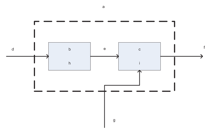
In this part, the Ising channel model is introduced. The channel is a unifilar FSC with feedback, as depicted in Fig. 1.

As mentioned before, the sets $\mathcal{X},\mathcal{Y},\mathcal{S}$ denote the input, output, and state alphabet, respectively. In the Ising channel model: $\mathcal{X}=\mathcal{Y}=\mathcal{S}=\{0,1\}$.

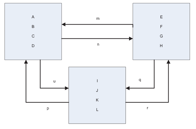
The Ising channel consists of two different topologies, as described in Fig. 2. The channel topologies depend on the channel state and are denoted by $Z$ and $S$. These $Z$ and $S$ notations are compatible with the well known $Z$ and $S$ channels. The channel topology at time $t$ is determined by $s_{t-1}\in\{0,1\}$.

As shown in Fig. 2, if $s_{t-1}=1$, the channel is in the $Z$ topology; if $s_{t-1}=0$, the channel is in the $S$ topology. The channel state at time $t$ is defined as the input to the channel at time $t$, meaning $s_{t}=x_{t}$.

The channel input, $x_{t}$, and state, $s_{t-1}$, have a crucial effect on the output, $y_{t}$. If the input is identical to the previous state, i.e. $x_{t}=s_{t-1}$, then the output is equal to the input, $y_{t}=x_{t}$, with probability $1$; if $x_{t}\neq s_{t-1}$ then $y_{t}$ can be either $0$ or $1$, each with probability $0.5$. This effect is summarized in Table II.

We assume a communication settings that includes feedback. The feedback is with unity delay. Hence, the transmitter (encoder) knows at time $t$ the message $m$ and the feedback samples $y^{t-1}$. Therefore, the input of the channel, $x_{t}$, is a function of both the message and the feedback as shown in Fig. 1.

Here we introduce a formulation for average-reward dynamic programs. Each DP problem is defined by a septuple $(\mathcal{Z},\mathcal{U},\mathcal{W},F,P_{z},P_{w},g)$, where all the functions considered are assumed to be measurable:

• $\mathcal{Z}$

  : is a Borel space which contains the states.

• $F$

  : is the function for which the discrete-time dynamic system evolves according to. $z_{t}=F(z_{t-1},u_{t},w_{t}),t\in\mathbb{N}^{\geq 1}$ (where each state $z_{t}\in\mathcal{Z}$).

• $\mathcal{U}$

  : is a compact subset of a Borel space, which contains the actions $u_{t}$.

• $\mathcal{W}$

  : is a measurable space, which contains the disturbances $w_{t}$.

• $P_{z}$

  : is a distribution from which the initial state, $z_{0}$, is drawn.

• $P_{w}$

  : is the distribution for which each disturbance, $w_{t}$, is drawn in accordance with $P_{w}(\cdot|z_{t-1},u_{t})$, which depends only on the state $z_{t-1}$ and action $u_{t}$.

• $g$

  : is a bounded reward function.

We consider a discrete-time dynamic system evolving according to

The history, $h_{t}=(z_{0},w_{0},\ldots,w_{t-1})$, summarizes information available prior to the selection of the $t$th action. The action, $u_{t}$, is selected by a function, $\mu_{t}$, which maps histories to actions. In particular, given a policy, $\pi=\{\mu_{1},\mu_{2},\ldots\}$, actions are generated according to $u_{t}=\mu_{t}(h_{t})$.

The objective is to maximize the average reward, given a bounded reward function $g:\cal{Z}\times\cal{U}\rightarrow\mathbb{R}$. The average reward for a policy $\pi$ is defined by

where the subscript $\pi$ indicates that actions are generated by the policy $\pi=(\mu_{1},\mu_{2},\ldots)$. The optimal average reward is defined by $\rho^{*}=\sup_{\pi}\rho_{\pi}$.

An alternative characterization of the optimal average reward is offered by the Bellman Equation. This equation verifies that a given average reward is optimal. The result presented here encapsulates the Bellman Equation and can be found in [25].

In this section we associate the DP problem, which was discussed in the previous section, with the Ising channel. Using the notations previously defined, the state, $z_{t}$, would be the vector of channel state probabilities $[p(s_{t}=0|y^{t}),p(s_{t}=1|y^{t})]$. In order to simplify notations, we consider the state $z_{t}$ to be the first component; that is, $z_{t}:=p(s_{t}=0|y^{t})$. This comes with no loss of generality, since $p(s_{t-1}=0|y^{t-1})+p(s_{t-1}=1|y^{t-1})=1$. Hence, the second component can be derived from the first, since the pair sums to one. The action, $u_{t}$, is a $2\times 2$ stochastic matrix

The disturbance, $w_{t}$, is the channel output, $y_{t}$. The DP-Ising channel association is presented in Table III.

Note that given a policy $\pi=(\mu_{1},\mu_{2},\ldots)$, $p(s_{t}|y^{t})$ is given in (8) (as shown in [12]), where $\mathbf{1}(\cdot)$ is the indicator function. The distribution of the disturbance, $w_{t}$, is $p(w_{t}|z^{t-1},w^{t-1},u^{t})=p(w_{t}|z_{t-1},u_{t})$. Conditional independence from $z^{t-2}$ and $w^{t-1}$ given $z_{t-1}$ is due to the fact that the channel output is determined by the channel state and input.

The state evolves according to $z_{t}=F(z_{t-1},u_{t},w_{t})$, where we obtain the function $F$ explicitly using relations from (8) as follows:

These expressions can be simplified by defining

and, using the fact that $u_{t}(1,1)=1-u_{t}(1,2),u_{t}(2,2)=1-u_{t}(2,1)$, we have that

Note that $\gamma_{t},\delta_{t}$ are functions of $z_{t-1}$. As shown in (10), given $z_{t-1}$, the action $u_{t}$ defines the pair $(\gamma_{t},\delta_{t})$ and vice versa. From here on, we represent the actions in terms of $\gamma_{t}$ and $\delta_{t}$. Since $u_{t}$ is a stochastic matrix, we have the constraints $0\leq\delta_{t}\leq z_{t}$ and $0\leq\gamma_{t}\leq 1-z_{t}$.

After finding the channel state probability, we can formulate the DP operator (6). We consider the reward to be $g(z_{t-1},u_{t})=I(X_{t},S_{t-1};Y_{t}|y^{t-1})$. Note that if $g(z_{t-1},u_{t})=I(X_{t},S_{t-1};Y_{t}|y^{t-1})$ then using Theorem 3 we have that

First, we show that the reward function $I(X_{t},S_{t-1};Y_{t}|y^{t-1})$ is indeed a function of $u_{t}$ and $z_{t-1}$. To show this we note that

Recall that $p(y_{t}|x_{t},s_{t-1})$ is given by the channel model. Thus, the reward is dependent only on $p(s_{t-1}|y^{t-1})$ and $p(x_{t}|s_{t-1},y^{t-1})=u_{t}$. Since $p(s_{t-1}|y^{t-1})$ is given by $z_{t-1}$, we have that

is indeed a function of $u_{t}$ and $z_{t-1}$. Now we find $g(z_{t-1},u_{t})$ explicitly for the Ising channel:

Where $H_{b}(\cdot)$ denotes the binary entropy function. $(a)$ follows from Table IV where the conditional distribution $p(x_{t},s_{t-1},y_{t}|y^{t-1})$ is calculated using (13) and $(b)$ follows from the definition of $\delta$ and $\gamma$ given in (10) and the fact that $u_{t}$ is a stochastic matrix. Therefore, using (15) and (6), we write the DP operator explicitly:

where $(a)$ follows from the fact that in the Ising channel case, $\int P_{w}(dw|z,u)h(F(z,u,w))$ takes the form $\sum_{w=0,1}p(w|z,u)h(F(z,u,w))$ and $F(z,u,w)$ is calculated explicitly using (11). We have formulated an equivalent dynamic program problem and found the DP operator explicitly. The objective is to maximize the average reward $\rho_{\pi}$ over all policies $\pi$. According to Theorem 4, if we identify a scalar $\rho$ and bounded function $h$ that satisfies the Bellman Equation, $\rho+Th(z)=h(z)$, then $\rho$ is the optimal average reward and, therefore, the channel capacity.

The aim of the numerical solution is to obtain some basic knowledge of the bounded function, $h$, which satisfies the Bellman Equation. In order to do so, the Bellman equation is solved using a value iteration algorithm. The algorithm generates a sequence of iterations according to

where $T$ is the DP operator, as in (18), and $J_{0}=0$.

For each $k$ and $z$, $J_{k}(z)$ is the maximal expected reward over $k$ periods given that the system starts in state $z$. Since rewards are positive, $J_{k}(z)$ grows with $k$ for each $z$. For each $k$, we define a differential reward function, $h_{k}(z)\triangleq J_{k}(z)-J_{k}(0)$.

For the numerical analysis, the interval $[0,1]$ was represented with a $1000$ points grid. Furthermore, each interval, such as $\delta$, which is in $[0,z]$ and $\gamma$, which is in $[0,(1-z)]$, was also represented with a $1000$ points grid. Obviously, the result has limited accuracy due to machine error in representation of real numbers. The numerical solution after $20$ value iterations is shown in Fig. 3. This figure shows the $J_{20}(z)$ function and the corresponding policies, $\gamma^{*}(z)$ and $\delta^{*}(z)$. The policies are chosen numerically such that the equation $T_{\gamma^{*},\delta^{*}}h(z)\geq T_{\gamma,\delta}h(z)$ holds for all $\gamma,\delta$ on the grid, where $T_{\gamma,\delta}$ represents the DP operator restricted to the policy given by $\gamma,\delta$. Moreover, Fig. 3 shows the histogram of $z$, which represents the relative number of times each point has been occupied by a state $z$. These values of $z$ have been calculated using (9) over $250000$ iterations, where each iteration calculates the next point using (9). Each time a specific value of $z$ was visited the program adds to this value $\frac{1}{250000}$, which gives the relative frequency each point was visited.

Here, the numerical results are explored in order to obtain further information on the possible analytical solution. We denote the optimal actions with $\gamma^{*}(z),\delta^{*}(z)$. Moreover, $h^{*}(z)$ denotes the function $h(z)$ restricted to the policy $\gamma^{*},\delta^{*}$.

As we can clearly see from the histogram presented in Fig. 3, the states, $z$, alternate between four major points. These points, which are symmetric around $\frac{1}{2}$ and two of them are $0$ and $1$, are denoted by $z_{0},z_{1},z_{2},z_{3}$, where $z_{0}=0$ and $z_{3}=1$. In addition, the function $h^{*}(z)$ found numerically is assumed to be symmetric around $\frac{1}{2}$.

In order to find $z_{i},\quad i=0,1,2,3$, we define $\gamma^{*}_{0}=\gamma^{*}(z=0)=a$. The variables $z_{i},\gamma^{*}_{i}=\gamma^{*}(z_{i})$, and $\delta^{*}_{i}=\delta^{*}(z_{i})$ for $i=0,1,2,3$, are presented in Table V. These variables are written with respect to the unknown parameter, $a=\gamma^{*}_{0}=\gamma^{*}(z=0)$, using (11), and the following assumptions, which are based on Fig. 3: i) we assume that $\delta=z\quad\forall z\in[z_{0},z_{2}]$, and ii) we assume there is a symmetry relation, $\gamma^{*}(z)=\delta^{*}(1-z)$.

Using the numerical solution, we assume that $a\notin\{0,1\}$, which implies that $z_{1},z_{2}\notin\{0,1\}$. In addition, we assume that $z_{1}\leq z_{2}$ and hence $a\geq\frac{1}{3}$. There is no loss of generality here, since otherwise we could do the same analysis and switch between $z_{1}$ and $z_{2}$. Moreover, using (11) and basic algebra, one can notice that the selection of $\gamma^{*}_{i},\delta^{*}_{i}\quad i=0,1,2,3,$ as in Table.V, guarantees that the states, $z_{t}$, alternate between the points $z_{i}$. For example, in order to attain the $z_{i}$ points, (11) was used in the following way: if $z_{t-1}=0$ then we have that $\gamma^{*}_{0}=a,\delta^{*}_{0}=0$ which implies

1. -

   if $w_{t}=0$ then $z_{t}=1+\frac{\delta^{*}_{t}-z_{t-1}}{1+\delta^{*}_{t}-\gamma^{*}_{t}}=1+\frac{0}{1-a}=1$.

2. -

   if $w_{t}=1$ then $z_{t}=\frac{1-z_{t-1}-\gamma^{*}_{t}}{1+\gamma^{*}_{t}-\delta^{*}_{t}}=\frac{1-0-a}{1+a}=\frac{1-a}{1+a}$.

Now, if $z_{t-1}=\frac{1-a}{1+a}$, using the symmetry, we also have the point $z_{t}=1-\frac{1-a}{1+a}=\frac{2a}{1+a}$. Since $a\geq\frac{1}{3}$ we have $\frac{1-a}{1+a}\leq\frac{2a}{1+a}$. Thus, for any specific time $t$, $z_{t}\in\{z_{0}=0,z_{1}=\frac{1-a}{1+a},z_{2}=\frac{2a}{1+a},z_{3}=1\}$.

In addition, based on the numerical solution, we assume that $\gamma^{*}$ and $\delta^{*}$ can be approximated by straight lines. Therefore, the following expressions can be found:

Note that if a scalar, $\rho$, and a function, $h$, solve the Bellman Equation, so do $\rho$ and $h+c1$ for any scalar $c1$. Hence, with no loss of generality, we can assume $h^{*}(\frac{1}{2})=1$.

References

- [1] W. Lenz, “Beitrage zum verstandnis der magnetischen eigenschaften in festen korpern,” Physikalische Zeitschrift, vol. 21, 1920.
- [2] E. Ising, “Beitrag zur theorie des ferromagnetismus,” Zeitschrift for Physik A Hadrons and Nuclei, vol. 31, 1925.
- [3] L. Onsager, “Crystal statistics. i. a two-dimensional model with an order-disorder transition,” Phys. Rev., vol. 65, Feb 1944.
- [4] T. Berger and F. Bonomi, “Capacity and zero-error capacity of ising channels,” IEEE Transactions on Information Theory, vol. 36, no. 7, pp. 173–180, 1990.
- [5] S. Arimoto, “An algorithm for computing the capacity of arbitrary discrete memoryless channels,” IEEE Transactions on Information Theory, 1972.
- [6] R. Blahut, “Computation of channel capacity and rate-distortion functions,” IEEE Transactions on Information Theory, 1972.
- [7] C. E. Shannon, “Communication in the presence of noise,” Proceedings of the IRE, vol. 37, no. 1, pp. 10–21, 1949.
- [8] M. S. Pinsker, Information and Information Stability of Random Variables and Processes. Moskva: Izv. Akad. Nauk, 1960, translated by A. Feinstein, 1964.
- [9] Y. H. Kim, “Feedback capacity of the first-order moving average Gaussian channel,” IEEE Transactions on Information Theory, vol. 52, pp. 3063–3079, 2006.
- [10] A. Goldsmith and P. Varaiya, “Capacity, mutual information, and coding for finite-state Markov channels,” IEEE Transactions on Information Theory, vol. 4, pp. 868–886, 1996.
- [11] J. Chen and T. Berger, “The capacity of finite-state markov channels with feedback,” IEEE Transactions on Information Theory, march 2005.
- [12] H. H. Permuter, P. W. Cuff, B. Van-Roy, and T. Weissman, “Capacity of the trapdoor channel with feedback,” IEEE Transactions on Information Theory, vol. 54, pp. 3150–3165, 2008.
- [13] J. Messy, “Causality, feedback and directed information,” in IEEE International Symposium on Information Theory and Applications, 1990.
- [14] H. Marko, “The bidirectional communication theory- a generalization of information theory,” IEEE Transactions on Information Theory, vol. COM-21, pp. 1335–1351, 1973.
- [15] G. Kramer, “Capacity results for the discrete memoryless network,” IEEE Transactions on Information Theory, vol. IT-49, pp. 4–21, 2003.
- [16] Y. H. Kim, “A coding theorem for a class of stationary channels with feedback,” IEEE Transactions on Information Theory, vol. 25, pp. 1488–1499, April, 2008.
- [17] S. Tatikonda and S. Mitter, “The capacity of channels with feedback,” IEEE Transactions on Information Theory, jan. 2009.
- [18] H. H. Permuter, T. Weissman, and A. Goldsmith, “Finite state channels with time-invariant deterministic feedback,” IEEE Transactions on Information Theory, 2009.
- [19] H. H. Permuter, T. Weissman, and J. Chen, “Capacity region of the finite-state multiple access channel with and without feedback,” IEEE Transactions on Information Theory, vol. 55, pp. 2455–2477, 2009.
- [20] B. Shrader and H. Permuter, “Feedback capacity of the compound channel,” IEEE Transactions on Information Theory, vol. 55, no. 8, pp. 3629 –3644, 2009.
- [21] R. Dabora and A. Goldsmith, “The capacity region of the degraded finite-state broadcast channel,” IEEE Transactions on Information Theory, vol. 56, no. 4, pp. 1828 –1851, 2010.
- [22] H. H. Permuter and I. Naiss, “Extension of the blahut-arimoto algorithm for maximizing directed information,” 2010.
- [23] S. Yang, A. Kavcic, and S. Tatikonda, “Feedback capacity of finite-state machine channels,” IEEE Transactions on Information Theory, 2005.
- [24] R. G. Gallager, Information theory and reliable communication. New York: Wiley, 1968.
- [25] A. Arapostathis, V. S. Borkar, E. Fernandez-Gaucherand, M. K. Ghosh, and S. Marcus, “Discrete time controlled Markov processes with average cost criterion - a survey,” SIAM Journal of Control and Optimization, vol. 31, no. 2, pp. 282–344, 1993.
- [26] T. Cover, “Enumerative source encoding,” IEEE Transactions on Information Theory, vol. 19, Jan 1973.
- [27] H. Asnani, H. Permuter, and T. Weissman, “To feed or not to feed back,” 2010.
- [28] A. Anastasopoulos, “A sequential transmission scheme for unifilar finite-state channels with feedback based on posterior matching,” in IEEE International Symposium on Information Theory, 2012.
- [29] S. Boyd and L. Vandenberghe, Convex Optimization. New York, USA: Cambridge University Press, 2004.