Latent Multi-group Membership Graph Model
Abstract
We develop the Latent Multi-group Membership Graph (LMMG) model, a model of networks with rich node feature structure. In the LMMG model, each node belongs to multiple groups and each latent group models the occurrence of links as well as the node feature structure. The LMMG can be used to summarize the network structure, to predict links between the nodes, and to predict missing features of a node. We derive efficient inference and learning algorithms and evaluate the predictive performance of the LMMG on several social and document network datasets.
Keywords:
network model, latent group, node features, multi-group1 Introduction
Network data, such as social networks of friends, citation networks of documents, and hyper-linked networks of webpages, play an increasingly important role in modern machine learning applications. Analyzing network data provides useful predictive models for recommending new friends in social networks (Backstrom & Leskovec, 2011) or scientific papers in document networks (Nallapati et al., 2008; Chang & Blei, 2009).
Research on networks has focused on various models of network link structure. Latent variable models (Airoldi et al., 2007; Hoff et al., 2002; Kemp et al., 2006) decompose a network according to hidden patterns of connections between the nodes, while models based on Kronecker products (Leskovec et al., 2010; Kim & Leskovec, 2012; Kim & Leskovec, 2011a) accurately model the global network structure. Though powerful, these models account only for the structure of the network, while ignoring observed features of the nodes. For example, in social networks users have profile information, and in document networks each node also contains the text of the document that it represents. Such models can find patterns which account for the connections between nodes, but they cannot account for the node features.
Node features along with the links between them provide rich and complementary sources of information and should be used simultaneously for uncovering, understanding and exploiting the latent structure in the data. In this respect, we develop a new network model considering both the emergence of links of the network and the structure of node features such as user profile information or text of a document.
Considering both sources of data, links and node features, leads to more powerful models than those that only consider links. For example, given a new node with a few of its links, traditional network models provide a predictive distribution of nodes to which it might be connected. However, to predict links of a node, our model does not need to see any links of a node. It can predict links using only node’s features. For example, we can suggest user’s friendships based only on the profile information, or recommend hyperlinks of a webpage based only on its textual information. Moreover, given a new node and its links, our model also provides a predictive distribution of node features. This can be used to predict features of a node given its links or even predict missing or hidden features of a node given its links. For example, in our model user’s interests or keywords of a webpage can be predicted using only the connections of the network. Such predictions are out of reach for traditional models of networks.
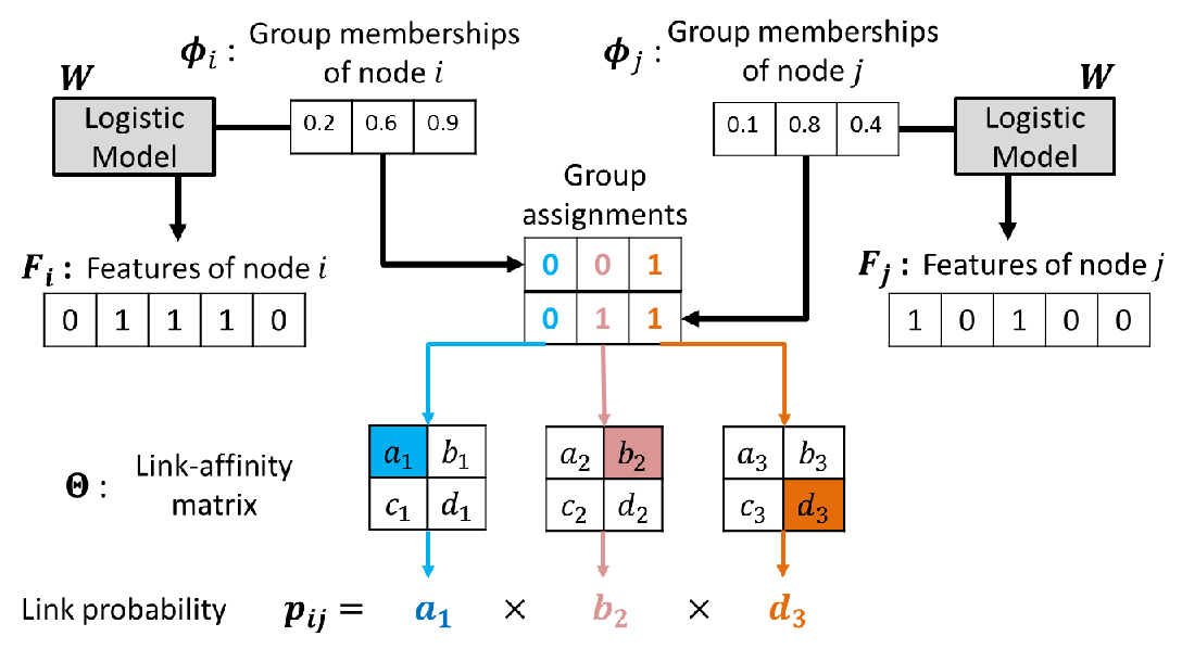
We develop a Latent Multi-group Membership Graph (LMMG) model of networks that explicitly ties nodes into groups of shared features and linking structure (Figure 1). Nodes belong to multiple latent groups and the occurrence of each node feature is determined by a logistic model based on the group memberships of the given node. Links of the network are then generated via link-affinity matrices. Each link-affinity matrix represents a table of link probabilities, and an appropriate entry of is chosen based on whether or not a pair of nodes share the membership in group . We derive effective algorithms for model parameter estimation and prediction. We study the performance of LMMG on real-world social and document networks. We investigate the predictive performance on three different tasks: link prediction, node feature prediction, and supervised node classification. The LMMG provides significantly better performance on all three tasks than natural alternatives and the current state of the art.
2 LMMG Model Formulation
The Latent Multi-group Membership Graph (LMMG) model is a model of a (directed or undirected) network and nodes which have categorical features. Our model contains two important ingredients or innovations (See Figure 1).
First, the model assigns nodes to latent groups and allows nodes to belong to multiple groups at once. In contrast to multinomial models of group membership (Airoldi et al., 2007; Chang & Blei, 2009), where the membership of a node is shared among the groups (the probability over group memberships of a node sums to 1), we model group memberships as a series of Bernoulli random variables ( in Figure 1), which indicates that nodes in our model can truly belong to multiple groups. Hence, in contrast to multinomial topic models, a higher probability of node membership to a group does not necessarily to lower probability of membership to some other group in the LMMG.
Second, for modeling the links of the network, each group has associated a link-affinity matrix ( in Figure 1). Each link-affinity matrix represents a table of link probabilities given that a pair of nodes belongs or does not belong to group . Thus, depending on the combination of the memberships of nodes to group , an appropriate element of is chosen. For example, the entry of captures the link-affinity when none of the nodes belongs to group , while stores the link-affinity when first node belongs to the group but the second does not. As we will later show that this allows for rich flexibility in modeling the links of the network as well as for uncovering and understanding the latent structure in the network data.
Now we formalize the LMMG model illustrated in Figure 2 and describe it in a generative way. Formally, each node has a real-valued group membership for each group . represents the probability that node belongs to group . Assuming the Beta distribution parameterized by as a prior distribution of group membership , we model the latent group assignment for each node as follows:
| (1) |
Since each group membership of a node is independent, a node can belong to multiple groups simultaneously.

The group memberships of a node affect both node features and its links. With respect to node features, we limit our focus to binary-valued features and use a logistic function to model the occurrence of node’s features based on the groups it belongs to. For each feature of node ( ), we consider a separate logistic model where we regard group memberships as input features of the model. In this way, the logistic model represents the relevance of each group membership to the presence of a node feature. For convenience, we refer to the input vector of node for the logistic model as , where represents the intercept term. Then,
| (2) |
where is the logistic model parameter for the -th node feature. The value of each indicates the contribution of group to the presence of node feature .
In order to model the links of the network, we build on the idea of the Multiplicative Attributes Random Graph (MAG) model (Kim & Leskovec, 2012). Here each latent group has associated a link-affinity matrix . Each entry of the link-affinity matrix indicates a tendency of linking between a pair of nodes depending on whether they belong to the group or not. In other words, given the group assignments and of nodes and , “selects” a row and “selects” a column of and so that the linking tendency from node to node is captured by . After acquiring such link-affinities from all the groups, we define the link probability as the product of the link-affinities. Therefore, based on latent group assignments and link-affinity matrices, we determine each entry of the adjacency matrix of the network as follows:
| (3) |
The network model parameter represents the link affinity with respect to the particular group . The model offers flexibility in a sense that we can represent many types of linking structures. In Figure 3, by varying the link-affinity matrix, the model can capture heterophily (love of the different), homophily (love of the same), or core-periphery structure. This way the affinity matrix allows us to discover the effects of node features on links of the network.
 |
 |
 |
| (a) Homophily | (b) Heterophily | (c) Core-periphery |
The node feature and the network models are connected via group memberships . For instance, suppose that is large for some feature and topic . Then, as the node belongs to topic with high probability ( is close to ), the feature of node , , is more likely to be . By modeling group memberships using multiple Bernoulli random variables (instead of using multinomial distribution (Airoldi et al., 2007; Chang & Blei, 2009)), we achieve greater modeling flexibility which allows for making predictions about links given features and features given links. In Section 4, we empirically demonstrate that the LMMG outperforms traditional models on these tasks.
Moreover, if we divide the nodes of the network into two sets depending on the membership to group , then we can discover how members of group link to other members as well as non-members of , based on the structure of . For example, when has large values on diagonal entries like in Figure 3(a), members or non-members are likely to link among themselves, while there is low affinity for links between members and non-members. Figure 3(b) captures exactly the opposite behavior where links are most likely between members and non-members. While the core-periphery structure is captured by link-affinity matrix in Figure 3(c) where nodes that share group memberships (the “core”) are most likely to link, while nodes in the periphery are least likely to link among themselves.
3 Inference, Estimation and Prediction
We now turn our attention to LMMG model estimation. Given a set of binary node features and the network , we aim to find node group memberships , parameters of node feature model, and link-affinity matrices .
3.1 Problem formulation
When the node features and the adjacency matrix are given, we aim to find the group memberships , the logistic model parameters , and the link-affinity matrices . We apply the maximum likelihood estimation, which finds the optimal values of , , and so that they maximize the likelihood where represents hyper parameters, , for the Beta prior distributioins. In the end, we aim to solve
| (4) |
Now we compute the objective function in the above optimization problem. Since the LMMG independently generates and given group memberships , we decompose the log-likelihood as follows:
| (5) |
Hence, to compute , we separately calculate each term of Equation (5). We obtain and from Equations (1) and (2):
where is defined in Equation (2).
With regard to the second term in Equation (5),
| (6) |
for . We note that is independent of given . To exactly calculate , we thus sum over every instance of given and , but this requires the sum over instances. As this exact computation is infeasible, we approximate using its lower bound obtained by applying Jensen’s Inequality to Equation (6):
| (7) |
Now that we are summing up over terms, the computation of the lower bound is feasible. We thus maximize the lower bound of the log-likelihood . To sum up, we aim to maximize
| (8) |
where , and . To avoid overfitting, we regularize the objective function by the L1-norm of .
3.2 Parameter estimation
To solve the problem in Equation (8), we alternately update the group memberships , the model parameters , and . Once , , and are initialized, we first update the group memberships to maximize with fixing and . We then update the model parameters and to minimize the function in Equation (8) by fixing . Note that is decomposed into , , and . Therefore, when updating and given , we separately maximize the corresponding log-likelihoods and . We repeat this alternate updating procedure until the solution converges. In the following we describe the details.
Update of group memberships . Now we focus on the update of group membership given the model parameters and . We use the coordinate ascent algorithm which updates each membership by fixing the others so to maximize the lower bound . By computing the derivatives of , , and we apply the gradient method to update each :
| (9) |
where is either or , and and is respectively defined in Equation (2) and (3). Due to the brevity, we describe the details of Equation (9) in the Appendix. Hence, by adding up , , and , we complete computing the derivative of the lower bound of log-likelihood and update the group membership using the gradient method:
| (10) |
for a given learning rate . By updating each in turn with fixing the others, we can find the optimal group memberships given the model parameters and .
Update of node feature model parameters . Now we update the parameters for node feature model, , while group memberships are fixed. Note that given the group membership the node feature model and the network model are independent of each other. Therefore, finding the parameter is identical to running the L1-regularized logistic regression given input and output data as we penalize the objective function in Equation (8) on the L1 value of the model parameter . We basically use the gradient method to update but make it sparse by applying the technique similar to LASSO:
| (11) |
if or where for and (i.e., we do not regularize on the intercepts). is a constant learning rate. Furthermore, if crosses while being updated, we assign to as LASSO does. By this procedure, we can update the node feature model parameter to maximize the lower bound of log-likelihood as well as to maintain the small number of relevant groups for each node feature.
Update of network model parameters . Next we focus on updating network model parameters, , also where the group membership is fixed. Again, note that the network model is independent of the node feature model given the group membership , so we do not need to consider or . We thus update to maximize given using the gradient method.
for a constant learning rate . We explain the computation of and in detail in the Appendix.
3.3 Prediction
With a fitted model, our ultimate goal is to make predictions about new data. In the real-world application, the node features are often missing. Our algorithm is able to nicely handle such missing node features by fitting LMMG only to the observed features. In other words, when we update the group membership or the feature model parameter by the gradient method from Equation (9) and (11), we only average the terms corresponding to the observed data. For example, when there is missing feature data, Equation (9) can be converted into as:
| (12) |
for the observed data .
Similarly, for link prediction we modify the model estimation method as follows. While updating the node feature model parameters based on the features of all the nodes including a new node, we estimate the network model parameters only on the observed network by holding out the new node. This way, the observed features naturally update the group memberships of a new node, we can predict the missing node features or network links by using the estimated group memberships and model parameters.
4 Experiments
Here we perform experiments to evaluate our model. First, we run the various prediction tasks: missing node feature prediction, missing link prediction, and supervised node classification. In all tasks our model outperforms natural baselines. Second, we qualitatively analyze the relationships between node features and network structure by a case study of a Facebook ego-network and show how the LMMG identifies useful and interpretable latent structures.
Datasets. For our experiments, we used the following datasets containing networks and node features.
- •
AddHealth (AH): School friendship network (458 nodes, 2,130 edges) with 35 school-related node features such as GPA, courses taken, and placement (Bearman et al., 1997).
- •
Egonet (EGO): Facebook ego-network of a particular user (227 nodes, 6,348 edges) and 14 binary features (e.g. same high school, same age, and sports club), manually assigned to each friend by the user.
- •
Facebook100 (FB): Facebook network of Caltech (769 nodes, 33,312 edges) and 24 university-related node features like major, gender, and dormitory (Traud et al., 2011).
- •
WebKB (WKB): Hyperlinks between computer science webpages of Cornell University in the WebKB dataset (195 nodes, 304 edges). We use occurrences of 993 words as binary features (Craven et al., 1998).
We binarized discrete valued features (e.g. school year) based on whether the feature value is greater than the median value. For the non-binary categorical features (e.g. major), we used an indicator variable for each possible feature value. Some of these datasets and the source code of our algorithms are available at http://snap.stanford.edu.
Predictive tasks. We investigate the predictive performance of the LMMG based on three different tasks. We visualize the three prediction tasks in Figure 4. Note that the column represents either features or nodes according to the type of the task. For each matrix, given 0/1 values in the white area, we predict the values of the entries with question marks. First, assuming that all node features of a given node are completely missing, we predict all the features based on the links of the node (Figure 4(a)). Second, when all the links of a given node are missing, we predict the missing links by using the node feature information (Figure 4(b)). Last, we assume only few features of a node are missing and we perform the supervised classification of a specific node feature given all the other node features and the network (Figure 4(c)).
 |
 |
 |
| (a) Missing feature | (b) Missing link | (c) Supervised node |
| prediction | prediction | classification |
Baseline models. Now we introduce natural baseline and state of the art methods. First, for the most basic baseline model, when predicting some missing value (node feature or link) of a given node, we average the corresponding values of all the other nodes and regard it as the probability of value . We refer to this algorithm as AVG. Second, as we can view each of the three prediction tasks as the classification task, we use Collective Classification (CC) algorithms that exploit both node features and network dependencies (Sen et al., 2008). For the local classifier of CC algorithms, we use Naive-Bayes (CC-N) as well as logistic regression (CC-L). We also compare the LMMG to the state or the art Relational Topic Model (RTM) (Chang & Blei, 2009). We give further details about these models and how they were applied in the Appendix.
Task 1: Predicting missing node features. First, we examine the performance for the task of predicting missing features of a node where features of other nodes and all the links are observed. We randomly select a node and remove all the feature values of that node and try to recover them. We quantify the performance by using the log-likelihood of the true feature values over the estimated distributions as well as the predictive accuracy (the probability of correctly predicting the missing features) of each method.
| LL | |||||
| AVG | CC-N | CC-L | RTM | LMMG | |
| AH | -23.0 | -17.6 | -16.8 | -63.4 | -15.6 |
| EGO | -5.4 | -6.6 | -5.1 | -9.9 | -3.7 |
| FB | -8.7 | -11.6 | -8.9 | -19.0 | -7.4 |
| WKB | -179.3 | -186.8 | -179.2 | -336.8 | -173.6 |
| ACC | |||||
| AVG | CC-N | CC-L | RTM | LMMG | |
| AH | 0.53 | 0.61 | 0.56 | 0.59 | 0.64 |
| EGO | 0.79 | 0.81 | 0.78 | 0.74 | 0.86 |
| FB | 0.77 | 0.76 | 0.75 | 0.77 | 0.80 |
| WKB | 0.88 | 0.88 | 0.89 | 0.88 | 0.90 |
Table 1 shows the results of the experiments by measuring the average of log-likelihood (LL) and prediction accuracy (ACC) for each algorithm and each dataset. We notice that LMMG model exhibits the best performance in the log-likelihood for all datasets. While CC-L in general performs the second best, our model outperforms it by up to 23%. The performance gain over the other models in terms of accuracy seems smaller when compared to the log-likelihood. However, LMMG model still predicts the missing node features with the highest accuracy on all datasets.
In particular, the LMMG exhibits the most improvement in node feature prediction on the ego-network dataset (30% in LL and 7% in ACC) over the next best method. As the node features are derived by manually labeling community memberships of each person in the ego-network dataset, a certain group of people in the network intrinsically share some node feature (community membership). In this sense, the node features and the links in the ego-network are directly related to each other and our model successfully exploits this relationship to predict missing node features.
Task 2: Predicting missing links. Second, we also consider the task of predicting the missing links of a specific node while the features of the node are given. Similarly to the previous task, we select a node at random, but here we remove all its links while observing its features. We then aim to recover the missing links. For evaluation, we use the log-likelihood (LL) of missing links as well as the area under the ROC curve (AUC) of missing link prediction.
| LL | |||||
| AVG | CC-N | CC-L | RTM | LMMG | |
| AH | -40.2 | -57.2 | -38.9 | -100.6 | -36.1 |
| EGO | -142.7 | -134.3 | -157.6 | -149.9 | -125.9 |
| FB | -320.8 | -330.7 | -345.6 | -359.1 | -328.3 |
| WKB | -54.2 | -185.5 | -39.6 | -25.8 | -13.7 |
| AUC | |||||
| AVG | CC-N | CC-L | RTM | LMMG | |
| AH | 0.51 | 0.69 | 0.39 | 0.56 | 0.72 |
| EGO | 0.61 | 0.89 | 0.55 | 0.49 | 0.89 |
| FB | 0.73 | 0.70 | 0.57 | 0.46 | 0.73 |
| WKB | 0.70 | 0.86 | 0.55 | 0.50 | 0.89 |
We give the experimental results for each dataset in Table 2. Again, the LMMG outperforms the baseline models in the log-likelihood except for the Facebook100 data. Interestingly, while RTM was relatively competitive when predicting missing features, it tends to fail predicting missing links, which implies that the flexibility of link-affinity matrices is needed for accurate modeling of the links.
We observe that Collective Classification methods look competetive in some performance metrics and datasets. For example, CC-N gives good results in terms of classification accuracy, and CC-L performs well in terms of the log-likelihood. As CC-N is a discriminative model, it does not perform well in missing link probability estimation. However, the LMMG is a generative model that produces a joint probability of node features and network links, so it is also very good at estimating missing links. Hence, in overall, the LMMG nicely exploits the relationship between the network structure and node features to predict missing links.
Task 3: Supervised node classification. Finally, we examine the performance on the supervised classification task. In many cases, we aim to classify entities (nodes) based on their feature values under the supervised setting. Here the relationships (links) between the entities are also provided. For this experiment, we hold out one feature of nodes as the output class, regarding all other features of nodes and the network as input data. We divide the nodes into a 70% training and 30% test set. Similarly, we measure the average of the log-likelihood (LL) as well as the average classification accuracy (ACC) on the test set.
| LL | |||||
| AVG | CC-N | CC-L | RTM | LMMG | |
| AH | -84.5 | -486.6 | -60.5 | -236.0 | -55.3 |
| EGO | -24.8 | -54.0 | -22.2 | -41.7 | -21.2 |
| FB | -97.6 | -254.6 | -79.2 | -181.7 | -63.4 |
| WKB | -17.5 | -254.6 | -15.4 | -193.6 | -15.0 |
| ACC | |||||
| AVG | CC-N | CC-L | RTM | LMMG | |
| AH | 0.52 | 0.58 | 0.63 | 0.51 | 0.63 |
| EGO | 0.76 | 0.76 | 0.77 | 0.75 | 0.79 |
| FB | 0.69 | 0.71 | 0.77 | 0.72 | 0.77 |
| WKB | 0.82 | 0.81 | 0.84 | 0.84 | 0.85 |
We illustrate the performance of various models in Table 3. The LMMG model performs better than the other models in both the log-likelihood and the classification accuracy. It improves the performance by up to 20% in the log-likelihood and 5% in the classification accuracy. We also notice that exploiting the relationship between node features and global network structure can improve the performance on supervised node classification compared to the models focusing on the local network dependencies (e.g., Collective Classification methods).
Case study: Analysis of a Facebook ego-network. Now we qualitatively analyze the Facebook ego-network example to provide insights into the relationship between node features and network structure. We examine the estimated model parameters (for features) and (for network structure). By investigating model parameters ( and ), we can find not only what features are important for each group but also how each group affects the link structure.
We begin by introducing the user which we used to create a network between his Facebook friends. We asked our user to label each of his friends with a number of labels. He chose to use 14 different labels. They correspond to his high school (HS), undergraduate university (University), math olympiad camp (Camp), computer programming club (KProg) and work place (KComp) friends. The user also assigned labels to identify friends from his graduate program (CS) and university (ST), basketball (BasketBall) and squash (Squash) clubs, as well as travel mates (Travel), summer internship buddies (Intern), family (Family) and age group (Age).
We fit the LMMG to the ego-network and each friend’s memberships to the above communities. We obtained the model parameters and . For the validation procedure, we set the number of latent groups to since the previous prediction tasks worked well when . In Table 4, for each of latent groups, we represent the top 3 features with the largest absolute value of model parameter and the corresponding link-affinity matrices .
We begin by investigating the first group. The top three labels the most correlated to the first group are ST, Age, and Intern. However, notice that Intern is negatively correlated. This means that group 1 contains students from the same graduate school and age, but not people with whom our user worked together at the summer internship (even though they may be of the same school/age). We also note that exhibits homophily structure. From this we learn that summer interns, who met our Facebook user neither because of shared graduate school nor because of the age, form a group within which people are densely connected. On the other hand, people of the same age at the same university also exhibit the homophily, but are less densely connected with each other. Such variation in link density that depends on the group memberships agrees with our intuition. Those who worked at the same company actively interact with each other so almost everyone is linked in Facebook. However, as the group of people of the same university or age is large and each pair of people in that group does not necessarily know each other, the link affinity in this group is naturally smaller than in the intern’s group.
Similarly, groups 2 and 3 form the two sports groups (BasketBall, Squash). People are connected densely within each of the groups, but less connected to the outside of the groups. This is natural because the sports clubs make members actively interact with each other but do not necessarily make members interact with those not in the clubs. Furthermore, we notice that those who graduated from not only the same high school (HS) but also the same undergraduate school (University) form another community but the membership to high school is more important than to the undergraduate university (8.7 vs. 2.3).
However, for groups 4 and 5, we note that the corresponding link-affinity matrices are nearly flat (i.e. values are nearly uniform). This implies that groups 4 and 5 are related to general node features. In this sense, we hypothesize that features like CS, family, math camp, and the company, have relatively little effect on the network structure.
| Group | Top 1 | Top 2 | Top 3 | Link-affinity matrix |
|---|---|---|---|---|
| 1 | ST (9.0) | Age (4.5) | Intern (-3.7) | [0.67 0.08; 0.08 0.17] |
| 2 | HS (-8.7) | University (-2.3) | BasketBall (2.2) | [0.26 0.18; 0.18 0.38] |
| 3 | University (-7.1) | KorST (-2.6) | Squash (2.2) | [0.22 0.23; 0.23 0.32] |
| 4 | CS (7.3) | Family (7.0) | Camp (6.9) | [0.25 0.24; 0.24 0.27] |
| 5 | KComp (5.2) | KorST (4.4) | Intern (-3.8) | [0.29 0.22; 0.22 0.27] |
5 Related Work and Discussion
The LMMG builds on previous research in machine learning and network analysis. Many models have been developed to explain network link structure (Airoldi et al., 2007; Hoff et al., 2002; Kemp et al., 2006; Leskovec et al., 2010) and extensions that incorporate node features have also been proposed (Getoor et al., 2001; Kim & Leskovec, 2011b; Taskar et al., 2003). However, these models do not consider latent groups and thus cannot provide the benefits of dimensionality reduction or produce interpretable clusters useful for understanding network community structure.
The LMMG provides meaningful clustering of nodes and their features in the network. The network models of similar flavor have been proposed in the past (Airoldi et al., 2007; Hoff et al., 2002; Kemp et al., 2006), and some even incorporate node features (Chang & Blei, 2009; Nallapati et al., 2008; Miller et al., 2009). However, such models have been mainly developed for document networks where they assume the multinomial topic distributions for each word in the document. We extend this by learning a logistic model for occurrence of each feature based on node group memberships. To highlight the difference between the previous models and ours, since topic memberships in the above models are modeled by multinomial distributions, a node has a mass of 1 to split among various topics. In contrast, in the LMMG, a node can belong to multiple topics at once without any constraint.
While previous work tends to explore only the network or only the features, the LMMG jointly models both so that it can make predictions on one given the other. The LMMG models the interaction between links and group memberships via link-affinity matrices which provide great flexibility and interpretability of obtained groups and interactions.
The LMMG is a new probabilistic model of links and nodes in networks. It can be used for link prediction, node feature prediction and supervised node classification. We have demonstrated qualitatively and quantitatively that the LMMG proves useful for analyzing network data. The LMMG significantly improves on previous models, integrating both node-specific information and link structure to give better predictions.
Acknowledgments
Myunghwan Kim was supported by the Kwanjeong Educational Foundation fellowship. This research has been supported in part by NSF CNS-1010921, IIS-1016909, IIS-1149837, IIS-1159679, Albert Yu & Mary Bechmann Foundation, Boeing, Allyes, Samsung, Yahoo, Alfred P. Sloan Fellowship and the Microsoft Faculty Fellowship.
References
- Airoldi et al. (2007) Airoldi, E. M., Blei, D. M., Fienberg, S. E., and Xing, E. P. Mixed membership stochastic blockmodels. JMLR, 9:1981–2014, 2007.
- Backstrom & Leskovec (2011) Backstrom, L. and Leskovec, J. Supervised random walks: Predicting and recommending links in social networks. In WSDM, 2011.
- Bearman et al. (1997) Bearman, P. S., Jones, J., and Udry, J. R. The national longitudinal study of adolescent health: Research design. http://www.cpc.unc.edu/addhealth, 1997.
- Chang & Blei (2009) Chang, J. and Blei, D. M. Relational topic models for document networks. In AISTATS, 2009.
- Craven et al. (1998) Craven, M., DiPasquo, D., Freitag, D., McCallum, A., Mitchell, T., Nigam, K., and Slattery, S. Learning to extract symbolic knowledge from the world wide web. In AAAI ’98, 1998.
- Getoor et al. (2001) Getoor, L., Segal, E., Taskar, B., and Koller, D. Probabilistic models of text and link structure for hypertext classification. In IJCAI Workshop on Text Learning: Beyond Supervision, 2001.
- Hoff et al. (2002) Hoff, P., Raftery, A., and Handcock, M. Latent space approaches to social network analysis. Journal of the American Statistical Association, 97:1090–1098, 2002.
- Kemp et al. (2006) Kemp, C., Tenebaum, J. B., and Griffiths, T. L. Learning systems of concepts with an infinite relational model. In AAAI ’06, 2006.
- Kim & Leskovec (2011a) Kim, M. and Leskovec, J. Network completion problem: Inferring missing nodes and edges in networks. In SDM, 2011a.
- Kim & Leskovec (2011b) Kim, M. and Leskovec, J. Modeling social networks with node attributes using the multiplicative attribute graph model. In UAI, 2011b.
- Kim & Leskovec (2012) Kim, M. and Leskovec, J. Multiplicative attribute graph model of real-world networks. Internet Mathematics, 8(1-2):113–160, 2012.
- Leskovec et al. (2010) Leskovec, J., Chakrabarti, D., Kleinberg, J., Faloutsos, C., and Ghahramani, Z. Kronecker Graphs: An Approach to Modeling Networks. JMLR, 11:985–1042, 2010.
- Miller et al. (2009) Miller, K. T., Griffiths, T. L., and Jordan, M. I. Nonparametric latent feature models for link prediction. In NIPS ’09, 2009.
- Nallapati et al. (2008) Nallapati, R., Ahmed, A., Xing, E., and Cohen, W. W. Joint latent topic models for text and citations. In KDD, 2008.
- Sen et al. (2008) Sen, P., Namata, G., Bilgic, M., Getoor, L., Gallagher, B., and Eliassi-rad, T. Collective classification in network data. AI Magazine, 29(3), 2008.
- Taskar et al. (2003) Taskar, B., Wong, M. F., Abbeel, P., and Koller, D. Link prediction in relational data. In NIPS, 2003.
- Traud et al. (2011) Traud, Amanda L., Mucha, Peter J., and Porter, Mason A. Social structure of facebook networks. Arxiv:CoRR, abs/1102.2166, 2011.
Appendix A Mathematical Details
A.1 Update of Group Membership
In Equation (9), we proposed the gradient ascent method which updates each group membership to maximize the lower bound of log-likelihood . To complete its computation, we further take a look at and in detail. Then, we can also compute and in the same way.
First, we calculate the derivative of expected log-likelihood for edges, . When all the group memberships except for are fixed, we can derive from definition of in Equation (3) as follows:
| (13) |
Here we use the following property. Since is an independent Bernoulli random variable with probability , for any function ,
| (14) |
Hence, by applying Equation (14) to (13), we obtain
| (15) |
Next, we compute the derivative of expected log-likelihood for unlinked node pairs, i.e. . Here we approximate the computation using the Taylor’s expansion, for small :
To compute ,
By Equation (14), each and its derivative can be obtained. Similarly, we can calculate , so we complete the computation of .
As we attain and , we eventually calculate . Hence, by adding up , , and , we complete computing the derivative of the lower bound of log-likelihood :
A.2 Update of MAG Model Parameters
Next we focus on the update of parameters of the network model, , where the group membership is fixed. Since the network model is independent of the node attribute model given the group membership , we do not need to consider , , or . We thus update to maximize only given using the gradient method.
As we previously did in computing by separating edge and non-edge terms, we compute each for and . To describe mathematically,
| (16) |
Appendix B Implementation Details
B.1 Initialization
Since the objective function in Equation (8) is non-convex, the final solution might be dependent on the initial values of , , and . For reasonable initialization, as the node attributes are given, we run the Singular Vector Decomposition (SVD) by regarding as an matrix and obtain the singular vectors corresponding to the top singular values. By taking the top components, we can approximate the node attributes over latent dimensions. We thus assign the -th entry of the -th right singular vectors multiplied by the -th singular value into for and . We also initialize each group membership based on the -th entry of the -th left singular vectors. This approximation can in particular provide good enough initial values when the top singular values dominate the others. In order to obtain the sparse model parameter , we reassign to of small absolute value such that .
Finally, to initialize the link-affinity matrices , we introduce the following way. When initializing the -th link-affinity matrix , we assume that the group other than group has nothing to do with network structure, i.e. every entry in the other link-affinity matrices has the equal value. Then, we compute the ratio between entries for as follows:
As the group membership is initialized above and and are independent of each other, we are able to compute the ratio between entries of . After computing the ratio between entries for each link-affinity matrix, we adjust the scale of the link-affinity matrices so that the expected number of edges in the MAG model is equal to the number of edges in the given network, i.e. .
B.2 Selection of the Number of Groups
Another issue in fitting the LMMG to the given network and node feature data is to determine the number of groups, . We can find the insight about the value of from the MAG model. It has been already proved that, in order for the MAG model to reasonably represent the real-world network, the value of should be in the order of where represents the number of nodes in the network (Kim & Leskovec, 2012). Since in the LMMG the network links are modeled similarly to the MAG model, the same argument on the number of groups still holds.
However, the above argument cannot determine the specific value of . To select one value of , we use the cross-validation method as follows. For instance, suppose that we aim to predict all the features of a node where its links to the other nodes are fully observed (Task 1 in Section 4). While holding out the test node, we can set up the same prediction task in a way that we select one at random from the other nodes (training nodes) and regard it as the validation test node. We then perform the missing node feature prediction on this validation node and obtain the log-likelihood result. By running this procedure with varying the validation test node, we can attain the average log-likelihood on the missing node features given the specific value of (i.e. N-fold cross-validation). Finally, we compare the average log-likelihood values according the value of and pick up the best one to maximize the log-likelihood. This method can be done by the other prediction tasks, missing link prediction and supervised node classification.
B.3 Baseline Models
Here we briefly describe how we implemented each baseline method depending on the type of prediction task.
AVG. In this baseline method, we regard each -th node feature and a link to the -th node as an independent random variable, respectively. In other words, we assume that missing node features or links do not depend on each other. Hence, we predict the -th missing node feature by finding the probability that the -th node feature of all the other nodes have value . We then regard the found probability as that of the missing -th node feature taking value .
Similarly, when we predict missing links (in particular, the link to the -th node) of a given node, we average the probability that all the other nodes are linked to the -th node and take it as the probability of link from the given node to the -th node (i.e. preferential attachment).
CC-N. For this method, we basically use the Naive-Bayes method using node features of each node as well as those of neighboring nodes. To represent each node feature of neighboring nodes by a single value, we select the majority value (either 0 or 1) from the neighbors’ feature values.
However, we cannot use the node features when predicting all the node features of a given node. Furthermore, the node features of neighboring nodes are unattainable when we predict missing links. Therefore, depending on the type of prediction task, we exploit only achievable information among node features and those of neighboring nodes.
CC-L. We employ the similar approach to the CC-N. However, here we use the logistic regression rather than the Naive-Bayes and average the feature values of neighboring nodes rather than pick up the majority value.
RTM. We use the lda-R package to run RTM (http://cran.r-project.org/web/packages/lda/index.html).