跳到论文正文
W Papers独立论文阅读器 arXiv:1205.4500 论文正文 计算阅读时间 · 0%
引用这篇论文根据当前论文元数据生成,正式投稿前建议核对。


License: arXiv.org perpetual non-exclusive license
arXiv:1205.4500v1 [math.NA] 21 May 2012

Structured conditioning of Hamiltonian eigenvalue problems

Paolo Buttà Address: Paolo Buttà, Dipartimento di Matematica, SAPIENZA Università di Roma, P.le Aldo Moro 5, 00185 Roma, Italy Email address: butta@mat.uniroma1.it and Silvia Noschese Address: Silvia Noschese, Dipartimento di Matematica, SAPIENZA Università di Roma, P.le Aldo Moro 5, 00185 Roma, Italy Email address: noschese@mat.uniroma1.it
Abstract.

We discuss the effect of structure-preserving perturbations on complex or real Hamiltonian eigenproblems and characterize the structured worst-case effect perturbations. We derive significant expressions for both the structured condition numbers and the worst-case effect Hamiltonian perturbations. It is shown that, for purely imaginary eigenvalues, the usual unstructured perturbation analysis is sufficient.

Key words and phrases: 
Structure eigenvalue problem, condition number, Hamiltonian structure.
2010 Mathematics Subject Classification
65F15, 65F35.

1. Introduction

For structured eigenvalue problems, algorithms that preserve the underlying matrix structure may improve the accuracy and efficiency of the eigenvalue computation and preserve possible eigenvalue symmetries in finite-precision arithmetic. The concept of backward stability, i.e., the requirement that the computed eigenvalues are the exact eigenvalues of a slightly perturbed matrix, is extended by requiring the perturbed matrix to have the same structure as the original one [B87]. In order to assess the strong numerical backward-stability of the employed structured algorithm and not to overestimate the worst-case effect of perturbations, it is appropriate to consider suitable measures of the sensitivity of the eigenvalues to perturbations of the same structure.

Our analysis is based on the perturbation expansion of a simple eigenvalue. The structured condition number of an eigenvalue λ∈A\lambda\in A is indeed a first-order measure of the worst-case effect on λ\lambda of perturbations of the same structure as AA. The structured conditioning measures we deal with can be computed endowing the subspace of matrices with the Frobenius norm; see, e.g., [T03, KKT06, R06] and references therein.

Here we are concerned with the Hamiltonian eigenvalue problems. They arise from a number of applications, particularly in systems and control theory. Algorithms and applications of Hamiltonian eigenproblems are discussed, e.g., in [BKM05] and references therein.

We investigate the sensitivity of the eigenvalues of a complex [real] Hamiltonian matrix with respect to complex [real] Hamiltonian perturbations.

Attention has been paid to derive straightforwardly computable formulae, for both the structured condition numbers and the maximal structured perturbations, that result to be explicative of the relationship between unstructured and structured conditioning. It is well known, see, e.g., [W65], that the worst (unstructured) perturbation which may affect a simple eigenvalue λ\lambda of a given matrix AA arises under the action of the matrix y​x∗yx^{*}, with xx and yy corresponding right and left eigenvectors, normalized to have ‖x‖2=‖y‖2=1\left\|x\right\|_{2}=\left\|y\right\|_{2}=1. As a matter of fact, if we add the Hamiltonian-structure requirement, just as for sparsity-structures [NP06] or symmetry-patterns [NP07], we prove that the Hamiltonian matrix which yields the structured worst-case effect perturbation is the structured analogue of y​x∗yx^{*}, i.e. the normalized projection of y​x∗yx^{*} onto the space of the complex [real] Hamiltonian matrices. Notice that a further condition on the angle between the right and left eigenvectors is here required in the normalization.

The paper is organized as follows. Section 2 provides formulae for the eigenvalue structured condition numbers and for the maximal Hamiltonian perturbations. In Section 3, the real case is addressed. Numerical tests are presented in Section 4. Finally, conclusions are drawn in Section 5.

2. Eigenvalue structured conditioning of Hamiltonian matrices

We start with some notation and definitions. We denote by ℋℂ{{\mathcal{H}}}_{{\mathbb{C}}} the linear subspace of 2​n2n-dimensional complex Hamiltonian matrices, i.e.,

ℋℂ={Q∈ℂ2​n×2​n:Q​J=(Q​J)∗}={Q=(KML−K∗):K,L,M∈ℂn×n,L=L∗,M=M∗},\begin{split}{\mathcal{H}}_{{\mathbb{C}}}&=\left\{Q\in{\mathbb{C}}^{2n\times 2n}\colon QJ=(QJ)^{*}\right\}\\ &=\left\{Q=\begin{pmatrix}K&M\\ L&-K^{*}\end{pmatrix}\colon K,L,M\in{\mathbb{C}}^{n\times n}\;,\;L=L^{*}\;,\;M=M^{*}\right\}\;,\end{split}

where JJ is the fundamental symplectic matrix, i.e.,

J=(0In−In0),J=\begin{pmatrix}0&I_{n}\\ -I_{n}&0\end{pmatrix}\;,

with InI_{n} the n×nn\times n identity matrix. We observe that the Hamiltonian matrix QQ is uniquely determined by the 4​n24n^{2} real parameters given by the 2​n22n^{2} real and imaginary parts of the elements of KK, the 2​n2n (real) diagonal elements of L,ML,M, and the 2​n​(n−1)2n(n-1) real and imaginary parts of the elements of the strict lower triangular parts of L,ML,M.

Proposition 2.1.

The closest Hamiltonian matrix to a given matrix A=(A1A3A2A4)∈ℂ2​n×2​nA=\begin{pmatrix}A_{1}&A_{3}\\ A_{2}&A_{4}\end{pmatrix}\in{\mathbb{C}}^{2n\times 2n} with respect to the Frobenius norm is

A|ℋℂ=12​(A1−A4∗A3+A3∗A2+A2∗A4−A1∗)=12​(A+J​A∗​J).A|_{{\mathcal{H}}_{{\mathbb{C}}}}=\frac{1}{2}\begin{pmatrix}A_{1}-A_{4}^{*}&A_{3}+A_{3}^{*}\\ A_{2}+A_{2}^{*}&A_{4}-A_{1}^{*}\end{pmatrix}=\frac{1}{2}(A+JA^{*}J)\;.
Proof.

For Q=(KML−K∗)∈ℋQ=\begin{pmatrix}K&M\\ L&-K^{*}\end{pmatrix}\in{\mathcal{H}} we have

‖A−Q‖F2=‖K−A1‖F2+‖K+A4∗‖F2+‖L−A2‖F2+‖M−A3‖F2.\|A-Q\|_{F}^{2}=\|K-A_{1}\|_{F}^{2}+\|K+A_{4}^{*}\|_{F}^{2}+\|L-A_{2}\|_{F}^{2}+\|M-A_{3}\|_{F}^{2}\;.

Since L,ML,M are only requested to be Hermitian, it is known that the last two terms in the right-hand side are minimized for L=12​(A2+A2∗)L=\frac{1}{2}(A_{2}+A_{2}^{*}) and M=12​(A3+A3∗)M=\frac{1}{2}(A_{3}+A_{3}^{*}). On the other hand, the minimization of

G⁡(K)=‖K−A1‖F2+‖K+A4∗‖F2G(K)=\|K-A_{1}\|_{F}^{2}+\|K+A_{4}^{*}\|_{F}^{2}

leads to K=12​(A1−A4∗)K=\frac{1}{2}(A_{1}-A_{4}^{*}). The proposition is thus proved. ∎

To state the next results we need some additional notation and definitions. It will be useful the following characterization of the space of complex Hamiltonian matrices,

ℋℂ={H+iW:H∈ℋ,W∈𝒲},{{\mathcal{H}}}_{{\mathbb{C}}}=\left\{H+\mathrm{i}\,W\colon H\in{\mathcal{H}},\;\;W\in{\mathcal{W}}\right\}\;,

where ℋ{\mathcal{H}} [resp. 𝒲]{\mathcal{W}}] is the linear space of real Hamiltonian [resp. skew-Hamiltonian] matrices, i.e.,

ℋ={H∈ℝ2​n×2​n:H​J=(H​J)T},𝒲={W∈ℝ2​n×2​n:W​J=−(W​J)T}.\begin{split}{\mathcal{H}}&=\left\{H\in{\mathbb{R}}^{2n\times 2n}\colon HJ=(HJ)^{T}\right\}\;,\\ {\mathcal{W}}&=\left\{W\in{\mathbb{R}}^{2n\times 2n}\colon WJ=-(WJ)^{T}\right\}\;.\end{split}

In particular, if A=ℜ⁡(A)+i​ℑ⁡(A)A=\Re(A)+\rm i\Im(A) then A|ℋℂ=ℜ⁡(A)|ℋ+i​ℑ⁡(A)|𝒲A|_{{\mathcal{H}}_{{\mathbb{C}}}}=\Re(A)|_{{\mathcal{H}}}+\rm i\Im(A)|_{{\mathcal{W}}} where, for B∈ℝ2​n×2​nB\in{\mathbb{R}}^{2n\times 2n},

B|ℋ:=12​(B+J​BT​J)B|𝒲:=12​(B−J​BT​J).B|_{{\mathcal{H}}}:=\frac{1}{2}(B+JB^{T}J)\;\,\qquad B|_{{\mathcal{W}}}:=\frac{1}{2}(B-JB^{T}J)\;.

We finally introduce the normalized projection of a matrix AA onto ℋℂ{\mathcal{H}}_{{\mathbb{C}}} as

A|𝒩:=A|ℋℂ‖A|ℋℂ‖F.A|_{\mathcal{N}}:=\frac{A|_{{\mathcal{H}}_{{\mathbb{C}}}}}{\|A|_{{\mathcal{H}}_{{\mathbb{C}}}}\|_{F}}\;. (2.1)
Theorem 2.2.

Let λ\lambda be a simple eigenvalue of a Hamiltonian matrix QQ, with corresponding right and left eigenvectors xx and yy normalized to have

‖x‖2=‖y‖2=1,ℑ⁡(y∗​J​x)=0.\|x\|_{2}=\|y\|_{2}=1\;,\qquad\Im(y^{*}Jx)=0\;. (2.2)

Given any Hamiltonian matrix EE with ‖E‖F=1\|E\|_{F}=1, let λE​(t)\lambda_{E}(t) be an eigenvalue of Q+t​EQ+tE converging to λ\lambda as t→0t\to 0. Then,

|λ˙E(0)|≤max{|y∗​G​xy∗​x|:∥G∥F=1,G∈ℋℂ}=‖y​x∗|ℋℂ‖F|y∗​x|.|\dot{\lambda}_{E}(0)|\leq\max\left\{\left|\frac{y^{*}Gx}{y^{*}x}\right|\colon\|G\|_{F}=1,\,G\in{\mathcal{H}}_{{\mathbb{C}}}\,\right\}=\frac{\|yx^{*}|_{{\mathcal{H}}_{{\mathbb{C}}}}\|_{F}}{|y^{*}x|}\;. (2.3)

Moreover,

λ˙E​(0)=‖y​x∗|ℋℂ‖Fy∗​xifE=±y​x∗|𝒩.\dot{\lambda}_{E}(0)=\frac{\|yx^{*}|_{{\mathcal{H}}_{{\mathbb{C}}}}\|_{F}}{y^{*}x}\qquad\mathrm{if}\qquad E=\pm yx^{*}|_{{\mathcal{N}}}\;. (2.4)
Remark 2.3.

By standard perturbation theory, the variational estimate in (2.3) holds for any choice of the right and left eigenvectors xx and yy. Instead, the assumption (2.2) is needed for the explicit expressions of the maximum and of the maximizers to hold.

Proof of Theorem 2.2. We shall use the real scalar product ⟨A,B⟩:=Trace⁡(AT​B)\left\langle A,B\right\rangle:=\mathrm{Trace}(A^{T}B), A,B∈ℝ2​n×2​nA,B\in{\mathbb{R}}^{2n\times 2n}, note ‖A‖F=⟨A,A⟩\|A\|_{F}=\sqrt{\left\langle A,A\right\rangle}. Our target is to compute

argmax{|y∗(H+iW)x|:H∈ℋ,W∈𝒲,∥H∥F2+∥W∥F2=1}.\mathrm{argmax}\left\{|y^{*}(H+\mathrm{i}\,W)x|\colon\;H\in{\mathcal{H}}\;,\;W\in{\mathcal{W}}\;,\;\|H\|_{F}^{2}+\|W\|_{F}^{2}=1\right\}.

The requirement H∈ℋH\in{\mathcal{H}} means that H​JHJ is symmetric, i.e., it is orthogonal (w.r.t. the above scalar product) to the space of skew-symmetric matrices. Similarly, W∈𝒲W\in{\mathcal{W}} means that W​JWJ is orthogonal to the space of symmetric matrices. Therefore, we study the auxiliary (unconstrained) variational problem for the function

G⁡(H,W)=|y∗​(H+i​W)​x|2+λ⁡(‖H‖F2+‖W‖F2−1)+⟨Λ,H​J⟩+⟨Γ,W​J⟩,G(H,W)=|y^{*}(H+\mathrm{i}\,W)x|^{2}+\lambda(\|H\|_{F}^{2}+\|W\|_{F}^{2}-1)+\left\langle\Lambda,HJ\right\rangle+\left\langle\Gamma,WJ\right\rangle\;,

which depends on 4​n2+14n^{2}+1 Lagrange multipliers, precisely the real parameter λ\lambda, the skew-symmetric matrix Λ\Lambda, and the symmetric matrix Γ\Gamma. Such parameters will be eventually determined by requiring that the solution satisfies all the constraints.

It is now useful to introduce the matrices ξ=ℜ⁡(y​x∗)\xi=\Re(yx^{*}), η=ℑ⁡(y​x∗)\eta=\Im(yx^{*}), so that

y​x∗=ξ+i​η,y¯​xT=ξ−i​ηyx^{*}=\xi+\mathrm{i}\,\eta\;,\quad\bar{y}x^{T}=\xi-\mathrm{i}\,\eta

and therefore

y∗​(H+i​W)​x=Trace⁡((y¯​xT)T​(H+i​W))=Trace⁡((ξT−i​ηT)​(H+i​W))=⟨ξ,H⟩+⟨η,W⟩+i⁡(⟨ξ,W⟩−⟨η,H⟩).\begin{split}y^{*}(H+\mathrm{i}\,W)x&=\mathrm{Trace}((\bar{y}x^{T})^{T}(H+\mathrm{i}\,W))=\mathrm{Trace}((\xi^{T}-\mathrm{i}\,\eta^{T})(H+\mathrm{i}\,W))\\ &=\left\langle\xi,H\right\rangle+\left\langle\eta,W\right\rangle+\mathrm{i}\,(\left\langle\xi,W\right\rangle-\left\langle\eta,H\right\rangle)\;.\end{split}

Whence,

G⁡(H,W)=(⟨ξ,H⟩+⟨η,W⟩)2+(⟨ξ,W⟩−⟨η,H⟩)2+λ⁡(‖H‖F2+‖W‖F2−1)+⟨Λ,H​J⟩+⟨Γ,W​J⟩,\begin{split}G(H,W)&=(\left\langle\xi,H\right\rangle+\left\langle\eta,W\right\rangle)^{2}+(\left\langle\xi,W\right\rangle-\left\langle\eta,H\right\rangle)^{2}\\ &\quad+\lambda(\|H\|_{F}^{2}+\|W\|_{F}^{2}-1)+\left\langle\Lambda,HJ\right\rangle+\left\langle\Gamma,WJ\right\rangle\;,\end{split}

and, by (2.2), also noticing that y∗​J​x=Trace⁡(x​y∗​J)=⟨ξ,J⟩−i⁡⟨η,J⟩y^{*}Jx=\mathrm{Trace}(xy^{*}J)=\left\langle\xi,J\right\rangle-\mathrm{i}\,\left\langle\eta,J\right\rangle,

‖ξ‖F2+‖η‖F2=1,⟨η,J⟩=0.\|\xi\|_{F}^{2}+\|\eta\|_{F}^{2}=1\;,\qquad\left\langle\eta,J\right\rangle=0\;. (2.5)

We now look for the critical points of GG. The gradients ∇HG​(H,W)\nabla_{H}G(H,W), ∇WG​(H,W)\nabla_{W}G(H,W), expressed in the form of 2​n×2​n2n\times 2n matrices, read,

∇HG​(H,W)=2​a​ξ−2​b​η+2​λ​H+Λ​JT,∇WG​(H,W)=2​a​η+2​b​ξ+2​λ​W+Γ​JT,\begin{split}\nabla_{H}G(H,W)&=2a\xi-2b\eta+2\lambda H+\Lambda J^{T}\;,\\ \nabla_{W}G(H,W)&=2a\eta+2b\xi+2\lambda W+\Gamma J^{T}\;,\end{split}

where we introduced the scalar functions,

a=⟨ξ,H⟩+⟨η,W⟩,b=⟨ξ,W⟩−⟨η,H⟩.a=\left\langle\xi,H\right\rangle+\left\langle\eta,W\right\rangle\;,\qquad b=\left\langle\xi,W\right\rangle-\left\langle\eta,H\right\rangle\;.

The critical points (H,W)(H,W) are therefore solutions to

H=−aλ​ξ+bλ​η−12​λ​Λ​JT,W=−aλ​η−bλ​ξ−12​λ​Γ​JT.\begin{split}H&=-\frac{a}{\lambda}\xi+\frac{b}{\lambda}\eta-\frac{1}{2\lambda}\Lambda J^{T}\;,\\ W&=-\frac{a}{\lambda}\eta-\frac{b}{\lambda}\xi-\frac{1}{2\lambda}\Gamma J^{T}\;.\end{split} (2.6)

By imposing H​J=(H​J)THJ=(HJ)^{T} and W​J=−(W​J)TWJ=-(WJ)^{T}, using that Λ=−ΛT\Lambda=-\Lambda^{T}, Γ=ΓT\Gamma=\Gamma^{T}, and recalling that J​JT=IJJ^{T}=I, JT=−JJ^{T}=-J, we get,

Λ=−a⁡(ξ​J+J​ξT)+b⁡(η​J+J​ηT),Γ=−a⁡(η​J−J​ηT)−b⁡(ξ​J−J​ξT).\Lambda=-a(\xi J+J\xi^{T})+b(\eta J+J\eta^{T})\;,\quad\Gamma=-a(\eta J-J\eta^{T})-b(\xi J-J\xi^{T})\;.

Plugging these expressions in (2.6) and calling α=−λ−1​a\alpha=-\lambda^{-1}a, β=λ−1​b\beta=\lambda^{-1}b, we conclude that the critical points have to be of the following form,

H=α⁡(ξ+J​ξT​J)+β⁡(η+J​ηT​J),W=α⁡(η−J​ηT​J)−β⁡(ξ−J​ξT​J).\begin{split}H&=\alpha(\xi+J\xi^{T}J)+\beta(\eta+J\eta^{T}J)\;,\\ W&=\alpha(\eta-J\eta^{T}J)-\beta(\xi-J\xi^{T}J)\;.\end{split} (2.7)

To determine the (still) unknown real parameters (α,β)(\alpha,\beta), it remains to maximize |y∗​(H+i​W)​x|2|y^{*}(H+\mathrm{i}\,W)x|^{2} with the constraint ‖H‖F2+‖W‖F2=1\|H\|_{F}^{2}+\|W\|_{F}^{2}=1 for (H,W)(H,W) as in (2.7). To compute these quantities we first notice that, as (ξT±i​ηT)​J(\xi^{T}\pm\mathrm{i}\,\eta^{T})J are rank-one (complex) matrices,

OPENTrace⁡((ξT+i​ηT)​J​(ξT±i​ηT)​J)=Trace⁡((ξT+i​ηT)​J)​Trace​(ξT±i​ηT)​J),\mathrm{Trace}((\xi^{T}+\mathrm{i}\,\eta^{T})J(\xi^{T}\pm\mathrm{i}\,\eta^{T})J)=\mathrm{Trace}((\xi^{T}+\mathrm{i}\,\eta^{T})J)\mathrm{Trace}(\xi^{T}\pm\mathrm{i}\,\eta^{T})J)\;,

from which, by identifying the real and imaginary parts, we get

Trace⁡(ξT​J​ξT​J)=Trace(ξTJ)2,Trace(ηTJηTJ)=Trace(ηTJ)2,Trace⁡(ξT​J​ηT​J)=Trace⁡(ηT​J​ξT​J)=Trace⁡(ηT​J)​Trace​(ξT​J).\begin{split}\mathrm{Trace}(\xi^{T}J\xi^{T}J)&=\mathrm{Trace}(\xi^{T}J)^{2}\;,\quad\mathrm{Trace}(\eta^{T}J\eta^{T}J)=\mathrm{Trace}(\eta^{T}J)^{2}\;,\\ \mathrm{Trace}(\xi^{T}J\eta^{T}J)&=\mathrm{Trace}(\eta^{T}J\xi^{T}J)=\mathrm{Trace}(\eta^{T}J)\mathrm{Trace}(\xi^{T}J)\;.\end{split}

Therefore, by (2.5),

⟨ξ,J​ξT​J⟩=⟨ξ,J⟩2,⟨η,JηTJ⟩=⟨η,J⟩2=0,⟨ξ,J​ηT​J⟩=⟨η,J​ξT​J⟩=⟨ξ,J⟩​⟨η,J⟩=0,\begin{split}\left\langle\xi,J\xi^{T}J\right\rangle&=\left\langle\xi,J\right\rangle^{2}\;,\quad\left\langle\eta,J\eta^{T}J\right\rangle=\left\langle\eta,J\right\rangle^{2}=0\;,\\ \left\langle\xi,J\eta^{T}J\right\rangle&=\left\langle\eta,J\xi^{T}J\right\rangle=\left\langle\xi,J\right\rangle\left\langle\eta,J\right\rangle=0\;,\end{split}

so that, one easily computes,

|y∗​(H+i​W)​x|2=(1+⟨ξ,J⟩2)2​α2+(1−⟨ξ,J⟩2)2​β2,|y^{*}(H+\mathrm{i}\,W)x|^{2}=(1+\left\langle\xi,J\right\rangle^{2})^{2}\alpha^{2}+(1-\left\langle\xi,J\right\rangle^{2})^{2}\beta^{2}\;,
‖H‖F2+‖W‖F2=2​(1+⟨ξ,J⟩2)​α2+2​(1−⟨ξ,J⟩2)​β2.\|H\|_{F}^{2}+\|W\|_{F}^{2}=2(1+\left\langle\xi,J\right\rangle^{2})\alpha^{2}+2(1-\left\langle\xi,J\right\rangle^{2})\beta^{2}\;. (2.8)

Moreover, as y​x∗|ℋyx^{*}|_{{\mathcal{H}}} [resp. (i​y​x)∗|ℋ(\mathrm{i}\,yx)^{*}|_{{\mathcal{H}}}] is given by (2.7) for (α,β)=(1/2,0)(\alpha,\beta)=(1/2,0) [resp. (α,β)=(0,1/2)(\alpha,\beta)=(0,1/2)], by (2.8) we get

‖y​x∗|ℋ‖F2=1+⟨ξ,J⟩22,‖(i​y​x)∗|ℋ‖F2=1−⟨ξ,J⟩22.\|yx^{*}|_{{\mathcal{H}}}\|_{F}^{2}=\frac{1+\left\langle\xi,J\right\rangle^{2}}{2}\;,\quad\|(\mathrm{i}\,yx)^{*}|_{{\mathcal{H}}}\|_{F}^{2}=\frac{1-\left\langle\xi,J\right\rangle^{2}}{2}\;.

If ‖(i​y​x)∗|ℋ‖>0\|(\mathrm{i}\,yx)^{*}|_{{\mathcal{H}}}\|>0, i.e., |⟨ξ,J⟩|<1|\left\langle\xi,J\right\rangle|<1, the (constrained) maximum of |y∗​(H+i​W)​x|2|y^{*}(H+\mathrm{i}\,W)x|^{2} is reached for α2=[2​(1+⟨ξ,J⟩2)]−1\alpha^{2}=[2(1+\left\langle\xi,J\right\rangle^{2})]^{-1} and β2=0\beta^{2}=0, so that the maximal perturbation is obtained for

E±=±ξ+J​ξT​J2​(1+⟨ξ,J⟩2)±i​η−J​ηT​J2​(1+⟨ξ,J⟩2)=±y​x∗|𝒩.E_{\pm}=\pm\frac{\xi+J\xi^{T}J}{\sqrt{2(1+\left\langle\xi,J\right\rangle^{2})}}\pm\mathrm{i}\,\frac{\eta-J\eta^{T}J}{\sqrt{2(1+\left\langle\xi,J\right\rangle^{2})}}=\pm yx^{*}|_{{\mathcal{N}}}\;.

On the other hand, if ‖(i​y​x)∗|ℋ‖=0\|(\mathrm{i}\,yx)^{*}|_{{\mathcal{H}}}\|=0 then α2=[2​(1+⟨ξ,J⟩2)]−1\alpha^{2}=[2(1+\left\langle\xi,J\right\rangle^{2})]^{-1} and H+i​W=E±H+\mathrm{i}\,W=E_{\pm} holds trivially. In both cases,

|y∗​E±​x|=1+⟨ξ,J⟩22=‖y​x∗|ℋ‖F.|y^{*}E_{\pm}x|=\sqrt{\frac{1+\left\langle\xi,J\right\rangle^{2}}{2}}=\|yx^{*}|_{{\mathcal{H}}}\|_{F}\;.

The theorem is thus proved. ∎

Remark 2.4.

By Theorem 2.2 the structured condition number is explicitly given by

κℋℂ​(λ)=‖y​x∗|ℋ‖F|y∗​x|,\kappa_{{\mathcal{H}}_{{\mathbb{C}}}}(\lambda)=\frac{\|yx^{*}|_{{\mathcal{H}}}\|_{F}}{|y^{*}x|}\;,

which can be also used for the structured backward error analysis of the algorithms in [BMX98, BK05]. Since the (unstructured) condition number of a simple eigenvalue is κ⁡(λ)=‖y​x∗‖F/|y∗​x|\kappa(\lambda)=\|yx^{*}\|_{F}/|y^{*}x|, we have κℋℂ​(λ)=κ⁡(λ)\kappa_{{\mathcal{H}}_{{\mathbb{C}}}}(\lambda)=\kappa(\lambda) if y​x∗yx^{*} is Hamiltonian. As shown in the next proposition, this can occur only if λ\lambda is a purely imaginary eigenvalue.

Proposition 2.5.

Let λ\lambda be a simple eigenvalue of a Hamiltonian matrix QQ with corresponding right and left eigenvectors xx and yy normalized such that ‖x‖2=‖y‖2=1\|x\|_{2}=\|y\|_{2}=1. If y​x∗yx^{*} is a Hamiltonian matrix or a skew-Hamiltonian matrix (i.e., (y​x∗​J)=−(y​x∗​J)∗(yx^{*}J)=-(yx^{*}J)^{*}) then ℜ⁡λ=0\Re\lambda=0.

Proof.

We prove the statement in the case y​x∗yx^{*} is a Hamiltonian matrix, the case y​x∗yx^{*} is skew-Hamiltonian can be treated similarly. We first show that if y​x∗yx^{*} is Hamiltonian then y=±J​xy=\pm Jx. Indeed, since JT=−JJ^{T}=-J, the identity y​x∗​J=(y​x∗​J)∗yx^{*}J=(yx^{*}J)^{*} can be recast as yk​(J​x¯)j=(J​x)k​y¯jy_{k}(J\bar{x})_{j}=(Jx)_{k}\bar{y}_{j} for any k,j=1,…,2​nk,j=1,\ldots,2n. As y∗​x≠0y^{*}x\neq 0, there exists at least one index kk for which (J​x)k,yk≠0(Jx)_{k},y_{k}\neq 0. Then, it is readily seen that the above identity implies J​x=c​yJx=cy for some c∈ℝc\in{\mathbb{R}}. As ‖x‖2=‖y‖2=1\|x\|_{2}=\|y\|_{2}=1, we conclude that y=±J​xy=\pm Jx. It remains to show that y=±J​xy=\pm Jx implies ℜ⁡λ=0\Re\lambda=0. To this end, it is enough to notice that, as QQ is Hamiltonian and J2=−1J^{2}=-1, the identity Q​x=λ​xQx=\lambda x can be recast as (J​x)∗​Q=−λ¯​(J​x)∗(Jx)^{*}Q=-\bar{\lambda}(Jx)^{*}. Since also y=±J​xy=\pm Jx is solution to y∗​Q=λ​y∗y^{*}Q=\lambda y^{*}, we conclude that λ+λ¯=0\lambda+\bar{\lambda}=0. ∎

3. Structured conditioning of real Hamiltonian eigenproblems

In several situations, we are interested in real structured perturbations of real Hamiltonian matrices. For these purposes, we are led to consider the real structured condition number κℋ​(λ)\kappa_{{\mathcal{H}}}(\lambda), where only real Hamiltonian perturbations are taken into account. For any smooth manifold 𝒮{\mathcal{S}}, an explicit formula for the real structured condition number κ𝒮​(λ)\kappa_{{\mathcal{S}}}(\lambda) is given in [KKT06, Eq. (2.16)]. Unfortunately, such formula, as its counterpart in the complex case, requires the characterization of the tangent space of 𝒮{\mathcal{S}} and the construction of a pattern matrix relevant to 𝒮{\mathcal{S}}. On the other hand, it yields the following bound,

κℋℂ​(λ)2≤κℋ​(λ)≤κℋℂ​(λ).\frac{\kappa_{{\mathcal{H}}_{{\mathbb{C}}}}(\lambda)}{\sqrt{2}}\leq\kappa_{{\mathcal{H}}}(\lambda)\leq\kappa_{{\mathcal{H}}_{{\mathbb{C}}}}(\lambda)\;.

Actually, we can give a more explicit expression of κℋ​(λ)\kappa_{{\mathcal{H}}}(\lambda), which is the content of the following theorem.

Theorem 3.1.

Let λ\lambda be a simple eigenvalue of a real Hamiltonian matrix QQ with corresponding right and left eigenvectors xx and yy normalized to have

‖x‖2=‖y‖2=1,ℑ⁡(y∗​J​x)​ℜ⁡(y∗​J​x)=Trace⁡(ℜ⁡(y​x∗)T​ℑ⁡(y​x∗)).\|x\|_{2}=\|y\|_{2}=1\;,\qquad\Im(y^{*}Jx)\,\Re(y^{*}Jx)=\mathrm{Trace}(\Re(yx^{*})^{T}\Im(yx^{*}))\;. (3.1)

Given any real Hamiltonian matrix EE with ‖E‖F=1\|E\|_{F}=1, let λE​(t)\lambda_{E}(t) be an eigenvalue of Q+t​EQ+tE converging to λ\lambda as t→0t\to 0. Then,

|λ˙E​(0)|≤max{|y∗​H​xy∗​x|:∥H∥F=1,H∈ℋ}=max⁡{‖ℜ⁡(y​x∗)|ℋ‖F|y∗​x|;∥ℑ(yx∗)|ℋ∥F}|y∗​x|}.\begin{split}|\dot{\lambda}_{E}(0)|&\leq\max\left\{\left|\frac{y^{*}Hx}{y^{*}x}\right|\colon\|H\|_{F}=1,\,H\in{\mathcal{H}}\,\right\}\\ &=\max\left\{\frac{\|\Re(yx^{*})|_{\mathcal{H}}\|_{F}}{|y^{*}x|};\frac{\|\Im(yx^{*})|_{\mathcal{H}}\|_{F}\}}{|y^{*}x|}\right\}\;.\end{split} (3.2)

Moreover:
1) if ‖ℜ⁡(y​x∗)|ℋ‖F>‖ℑ⁡(y​x∗)|ℋ‖F\|\Re(yx^{*})|_{\mathcal{H}}\|_{F}>\|\Im(yx^{*})|_{\mathcal{H}}\|_{F} then

λ˙E​(0)=‖ℜ⁡(y​x∗)|ℋ‖Fy∗​x𝑓𝑜𝑟E=±ℜ⁡(y​x∗)|ℋ∥ℜ(yx∗)|ℋ)∥F;\dot{\lambda}_{E}(0)=\frac{\|\Re(yx^{*})|_{\mathcal{H}}\|_{F}}{y^{*}x}\quad\mathit{for}\quad E=\pm\frac{\Re(yx^{*})|_{{\mathcal{H}}}}{\|\Re(yx^{*})|_{\mathcal{H}})\|_{F}}\;;

2) if ‖ℜ⁡(y​x∗)|ℋ‖F<‖ℑ⁡(y​x∗)|ℋ‖F\|\Re(yx^{*})|_{\mathcal{H}}\|_{F}<\|\Im(yx^{*})|_{\mathcal{H}}\|_{F} then

λ˙E​(0)=‖ℑ⁡(y​x∗)|ℋ‖Fy∗​x𝑓𝑜𝑟E=±ℑ⁡(y​x∗)|ℋ∥ℑ(yx∗)|ℋ)∥F;\dot{\lambda}_{E}(0)=\frac{\|\Im(yx^{*})|_{\mathcal{H}}\|_{F}}{y^{*}x}\quad\mathit{for}\quad E=\pm\frac{\Im(yx^{*})|_{{\mathcal{H}}}}{\|\Im(yx^{*})|_{\mathcal{H}})\|_{F}}\;;

3) if ‖ℜ⁡(y​x∗)|ℋ‖F=‖ℑ⁡(y​x∗)|ℋ‖F\|\Re(yx^{*})|_{\mathcal{H}}\|_{F}=\|\Im(yx^{*})|_{\mathcal{H}}\|_{F} then

λ˙E​(0)=‖ℜ⁡(y​x∗)|ℋ‖Fy∗​x𝑓𝑜𝑟​𝑎𝑛𝑦E=ℜ⁡(y​x∗)|ℋ​cos⁡θ+ℑ⁡(y​x∗)|ℋ​sin⁡θ‖ℜ⁡(y​x∗)|ℋ‖F,\dot{\lambda}_{E}(0)=\frac{\|\Re(yx^{*})|_{\mathcal{H}}\|_{F}}{y^{*}x}\quad\mathit{for}\;\mathit{any}\quad E=\frac{\Re(yx^{*})|_{{\mathcal{H}}}\cos\theta+\Im(yx^{*})|_{{\mathcal{H}}}\sin\theta}{\|\Re(yx^{*})|_{\mathcal{H}}\|_{F}}\;,

with θ∈[0,2​π]\theta\in[0,2\pi].

Proof.

Our target is to compute

argmax{|y∗Hx|:H∈ℋ,∥H∥F2=1}.\mathrm{argmax}\left\{|y^{*}Hx|\colon\;H\in{\mathcal{H}}\;,\;\|H\|_{F}^{2}=1\right\}.

As before, we introduce the real matrices ξ=ℜ⁡(y​x∗)\xi=\Re(yx^{*}), η=ℑ⁡(y​x∗)\eta=\Im(yx^{*}). By arguing as in the proof of Theorem 2.2, we find that the argmax have to be of the following form,

H=α⁡(ξ+J​ξT​J)+β⁡(η+J​ηT​J).H=\alpha(\xi+J\xi^{T}J)+\beta(\eta+J\eta^{T}J)\;. (3.3)

As ⟨ξ+J​ξT​J,η+J​ηT​J⟩=2​⟨ξ,η⟩+2​⟨ξ,J⟩​⟨η,J⟩\left\langle\xi+J\xi^{T}J,\eta+J\eta^{T}J\right\rangle=2\left\langle\xi,\eta\right\rangle+2\left\langle\xi,J\right\rangle\left\langle\eta,J\right\rangle and recalling y∗​J​x=⟨ξ,J⟩−i⁡⟨η,J⟩y^{*}Jx=\left\langle\xi,J\right\rangle-\mathrm{i}\,\left\langle\eta,J\right\rangle, by (3.1) we have,

‖ξ‖F2+‖η‖F2=1,⟨ξ+J​ξT​J,η+J​ηT​J⟩=0.\|\xi\|_{F}^{2}+\|\eta\|_{F}^{2}=1\;,\qquad\left\langle\xi+J\xi^{T}J,\eta+J\eta^{T}J\right\rangle=0\;.

Whence, a straightforward computation shows that if H=α⁡(ξ+J​ξT​J)+β⁡(η+J​ηT​J)H=\alpha(\xi+J\xi^{T}J)+\beta(\eta+J\eta^{T}J) then

|y∗​H​x|2=Dξ2​α2+Dη2​β2,‖H‖F2=2​Dξ​α2+2​Dη​β2,|y^{*}Hx|^{2}=D_{\xi}^{2}\alpha^{2}+D_{\eta}^{2}\beta^{2}\;,\quad\|H\|_{F}^{2}=2D_{\xi}\alpha^{2}+2D_{\eta}\beta^{2}\;,

where

Dξ:=12​‖ξ+J​ξT​J‖F2=‖ξ‖F2+⟨ξ,J⟩2,Dη:=12​‖η+J​ηT​J‖F2=‖η‖F2+⟨η,J⟩2.\begin{split}D_{\xi}&:=\frac{1}{2}\|\xi+J\xi^{T}J\|_{F}^{2}=\|\xi\|_{F}^{2}+\left\langle\xi,J\right\rangle^{2}\;,\\ D_{\eta}&:=\frac{1}{2}\|\eta+J\eta^{T}J\|_{F}^{2}=\|\eta\|_{F}^{2}+\left\langle\eta,J\right\rangle^{2}\;.\end{split}

Moreover, as ℜ⁡(y​x∗)|ℋ\Re(yx^{*})|_{\mathcal{H}} [resp. ℑ⁡(y​x∗|ℋ)\Im(yx^{*}|_{\mathcal{H}})] is given by (3.3) for (α,β)=(1/2,0)(\alpha,\beta)=(1/2,0) [resp. (α,β)=(0,1/2)(\alpha,\beta)=(0,1/2)], it follows that

‖ℜ⁡(y​x∗)|ℋ‖F2=Dξ2,‖ℑ⁡(y​x∗)|ℋ‖F2=Dη2.\|\Re(yx^{*})|_{\mathcal{H}}\|_{F}^{2}=\frac{D_{\xi}}{2}\;,\quad\|\Im(yx^{*})|_{\mathcal{H}}\|_{F}^{2}=\frac{D_{\eta}}{2}\;.

If both DξD_{\xi} and DηD_{\eta} are positive the (constrained) maximum of |y∗​H​x|2|y^{*}Hx|^{2} is reached for (α2,β2)=((2​Dξ)−1,0)(\alpha^{2},\beta^{2})=((2D_{\xi})^{-1},0) if Dξ>DηD_{\xi}>D_{\eta} and for (α2,β2)=(0,(2​Dη)−1)(\alpha^{2},\beta^{2})=(0,(2D_{\eta})^{-1}) if Dξ<DηD_{\xi}<D_{\eta}. In the critical case Dξ=Dη=:DD_{\xi}=D_{\eta}=:D, the function |y∗​H​x|2|y^{*}Hx|^{2} is constant and any pair (α2,β2)(\alpha^{2},\beta^{2}) satisfying the constraint 2​D​(α2+β2)=12D(\alpha^{2}+\beta^{2})=1 is allowed. Therefore, the maximal perturbation is obtained for

{Eξ=±ξ+J​ξT​J2​Dξif ​Dξ>Dη,Eη=±η+J​ηT​J2​Dηif ​Dξ<Dη,\begin{cases}{\displaystyle E_{\xi}=\pm\frac{\xi+J\xi^{T}J}{\sqrt{2D_{\xi}}}}&\text{if }D_{\xi}>D_{\eta}\;,\\ \\ {\displaystyle E_{\eta}=\pm\frac{\eta+J\eta^{T}J}{\sqrt{2D_{\eta}}}}&\text{if }D_{\xi}<D_{\eta}\;,\end{cases}

while, in the critical case Dξ=Dη=:DD_{\xi}=D_{\eta}=:D, for

Eθ=(ξ+J​ξT​J)​cos⁡θ+(η+J​ηT​J)​sin⁡θ2​D,θ∈[0,π].E_{\theta}=\frac{(\xi+J\xi^{T}J)\cos\theta+(\eta+J\eta^{T}J)\sin\theta}{\sqrt{2D}}\;,\quad\theta\in[0,\pi]\;.

On the other hand, if Dη=0D_{\eta}=0 [resp. Dξ=0D_{\xi}=0] then α2=(2​Dξ)−1\alpha^{2}=(2D_{\xi})^{-1} [resp. β2=(2​Dη)−1\beta^{2}=(2D_{\eta})^{-1}] and H=EξH=E_{\xi} [resp. H=EηH=E_{\eta}] holds trivially. In all cases,

|y∗​Eξ​x|=Dξ2,|y∗​Eη​x|=Dη2,|y∗​Eθ​x|=D2.|y^{*}E_{\xi}x|=\sqrt{\frac{D_{\xi}}{2}}\;,\quad|y^{*}E_{\eta}x|=\sqrt{\frac{D_{\eta}}{2}}\;,\quad|y^{*}E_{\theta}x|=\sqrt{\frac{D}{2}}\;.

The theorem is thus proved. ∎

Remark 3.2.

We observe that y​x∗yx^{*} is Hamiltonian if and only if ℑ⁡(y​x∗)|ℋ=0\Im(yx^{*})|_{\mathcal{H}}=0 and ℜ⁡(y​x∗)=ℜ⁡(y​x∗)|ℋ\Re(yx^{*})=\Re(yx^{*})|_{\mathcal{H}}. Likewise, y​x∗yx^{*} is skew-Hamiltonian if and only if ℜ⁡(y​x∗)|ℋ=0\Re(yx^{*})|_{\mathcal{H}}=0 and ℑ⁡(y​x∗)=ℑ⁡(y​x∗)|ℋ\Im(yx^{*})=\Im(yx^{*})|_{\mathcal{H}}. Therefore, by Theorem 3.1,

κℋ​(λ)={‖ℜ⁡(y​x∗)‖F|y∗​x|if​y​x∗​is Hamiltonian,‖ℑ⁡(y​x∗)‖F|y∗​x|if​y​x∗​is skew-Hamiltonian.\kappa_{\mathcal{H}}(\lambda)=\begin{cases}{\displaystyle\frac{\|\Re(yx^{*})\|_{F}}{|y^{*}x|}}&\mathrm{if}\;\;yx^{*}\;\;\mbox{is Hamiltonian}\;,\\ {\displaystyle\frac{\|\Im(yx^{*})\|_{F}}{|y^{*}x|}}&\mathrm{if}\;\;yx^{*}\;\;\mbox{is skew-Hamiltonian}\;.\end{cases}

By [BK03, Theorem 2.1] it follows that κℋ​(λ)\kappa_{\mathcal{H}}(\lambda) is equal to the real (unstructured) condition number. Moreover, by Proposition 2.5 this occurs only if λ\lambda is a purely imaginary eigenvalue.

Remark 3.3.

If is worthwhile to remark that if the eigenvalue λ\lambda is real, since the right and left eigenvectors are also real, then (2.2) and (3.1) are trivially satisfied and κℋ​(λ)=κℋℂ​(λ)\kappa_{{\mathcal{H}}}(\lambda)=\kappa_{{\mathcal{H}}_{{\mathbb{C}}}}(\lambda).

4. Numerical tests

Example 4.1. Consider the Hamiltonian matrix H=(H1H3H2H4)∈ℝ4×4H=\begin{pmatrix}H_{1}&H_{3}\\ H_{2}&H_{4}\end{pmatrix}\in{\mathbb{R}}^{4\times 4}, where

H1=(0200),H2=(−0.10.10.10.1),H3=(00.10.1−0.1).H_{1}=\begin{pmatrix}0&2\\ 0&0\end{pmatrix},\quad H_{2}=\begin{pmatrix}-0.1&0.1\\ \phantom{2}0.1&0.1\end{pmatrix},\quad H_{3}=\begin{pmatrix}0&\phantom{2}0.1\\ 0.1&-0.1\end{pmatrix}.

It is well known that if λ∈ℂ−(ℝ∪i​ℝ)\lambda\in{\mathbb{C}}-({\mathbb{R}}\cup\rm\mathrm{i}\,{\mathbb{R}}) is an eigenvalue of a real Hamiltonian matrix, then also −λ-\lambda, λ¯\overline{\lambda}, −λ¯-\overline{\lambda} are eigenvalues, since the spectrum is symmetric with respect to the real and the imaginary axis. According to Theorems 2.2 and 3.1, one derives for the eigenvalues of HH the condition numbers reported in Table 1.
λ\lambda κ⁡(λ)\kappa(\lambda) κℋℂ​(λ)\kappa_{{\mathcal{H}}_{{\mathbb{C}}}}(\lambda) κℋ​(λ)\kappa_{\mathcal{H}}(\lambda)
±0.3205±i​ 0.3126\pm 0.3205\pm\mathrm{i}\,0.3126 2.35132.3513 1.66311.6631 1.58511.5851
Table 1. Example 4.1. Unstructured, structured and real structured eigenvalue condition numbers.
Refer to caption
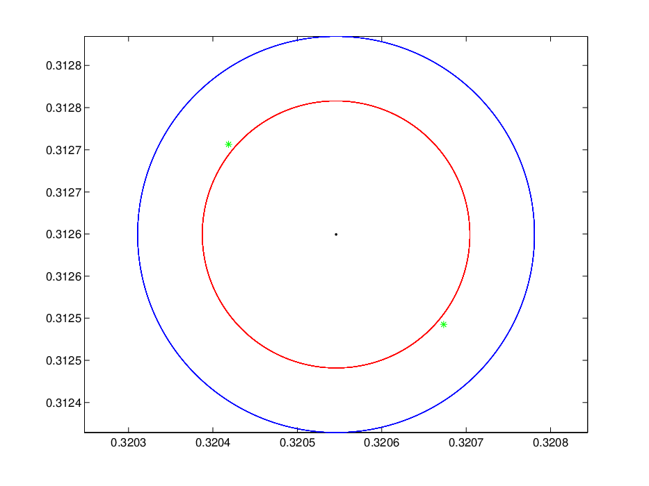
Figure 1. Example 4.1. Perturbations induced in the eigenvalue λ\lambda by the complex structured maximal perturbations (green ∗\ast), the real structured maximal perturbations (red −-) and the unstructured maximal perturbations (blu −-).

Let us focus on the eigenvalue λ=0.3205+i​ 0.3126\lambda=0.3205+\mathrm{i}\,0.3126, marked by a black point in Figure 1, and consider ε\varepsilon-norm perturbations, i.e. perturbation matrices of Frobenius norm equal to ε\varepsilon, with ε=10−4\varepsilon=10^{-4}.

The complex structured maximal perturbation matrices in (2.4) shift λ\lambda to one of the points marked by a green star in Figure 1. As a matter of fact, with respect to structured perturbations, the eigenvalue is not equally sensitive in any direction of the complex plane, since its eigenvectors have been normalized such that (2.2) is satisfied.

As for the real structured perturbations, holding in this case the equality ‖ℜ⁡(y​x∗)|ℋ‖F=‖ℑ⁡(y​x∗)|ℋ‖F\|\Re(yx^{*})|_{\mathcal{H}}\|_{F}=\|\Im(yx^{*})|_{\mathcal{H}}\|_{F}, the maximal perturbation matrices are given by case 3) in Theorem 3.1 and they shift λ\lambda to the boundary of the red circle of radius κℋ​(λ)​ε\kappa_{\mathcal{H}}(\lambda)\varepsilon.

We point out that the unstructured worst-case effect perturbation matrices ε​ei​θ​y​x∗\varepsilon\,\mathrm{e}^{\mathrm{i}\,\theta}yx^{*}, for θ∈[0,2​π]\theta\in[0,2\pi], shift in their turn λ\lambda to the boundary of the blue circle of radius κ⁡(λ)​ε\kappa(\lambda)\varepsilon. Analogous results hold for the other three eigenvalues of HH.

Example 4.2. Consider the same Hamiltonian test matrix as in Example 4.1, except for the block H3H_{3} that is here multiplied by the factor 0.10.1.

λ\lambda κ⁡(λ)\kappa(\lambda) κℋℂ​(λ)\kappa_{{\mathcal{H}}_{{\mathbb{C}}}}(\lambda) κℋ​(λ)\kappa_{\mathcal{H}}(\lambda)
±0.1786±i​ 0.1771\pm 0.1786\pm\mathrm{i}\,0.1771 7.02637.0263 6.37696.3769 6.31846.3184
Table 2. Example 4.2. Unstructured, structured and real structured eigenvalue condition numbers.
Refer to caption
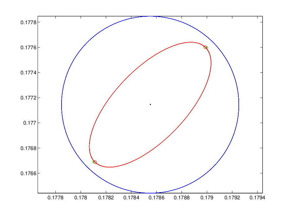
Figure 2. Example 4.2. Perturbations induced in λ\lambda by the complex structured (green ∗\ast), real structured (red ∘\circ) and unstructured (blu −-) maximal perturbations, and by the real structured perturbations in (4.1) (red −-).

We consider ε\varepsilon-norm perturbations in the matrix and analyze the effects induced in λ=0.1786+i​ 0.1771\lambda=0.1786+\mathrm{i}\,0.1771. The complex [real] structured maximal perturbation matrices shift λ\lambda to one of the points marked by a green star [red circlet] in Figure 2. Since ‖ℜ⁡(y​x∗)|ℋ‖F<‖ℑ⁡(y​x∗)|ℋ‖F\|\Re(yx^{*})|_{\mathcal{H}}\|_{F}<\|\Im(yx^{*})|_{\mathcal{H}}\|_{F}, case 2) in Theorem 3.1 holds; nevertheless, for the sake of completeness, let us take into account even the (non-maximal) real Hamiltonian matrices

Eθ=ℜ⁡(y​x∗)|ℋ​cos⁡θ+ℑ⁡(y​x∗)|ℋ​sin⁡θ‖ℜ⁡(y​x∗)|ℋ​cos⁡θ+ℑ⁡(y​x∗)|ℋ​sin⁡θ‖F,E_{\theta}=\frac{\Re(yx^{*})|_{{\mathcal{H}}}\cos\theta+\Im(yx^{*})|_{{\mathcal{H}}}\sin\theta}{\|\Re(yx^{*})|_{{\mathcal{H}}}\cos\theta+\Im(yx^{*})|_{{\mathcal{H}}}\sin\theta\|_{F}}\;, (4.1)

and notice that the perturbation matrices ε​Eθ\varepsilon\,E_{\theta}, for θ∈[0,2​π]\theta\in[0,2\pi], have the effect of shifting λ\lambda to the boundary of the ellipse in Figure 2, whose major axis gives indeed the direction induced by the worst-case effect perturbations.

5. Conclusions

We have derived simple expressions for structured eigenvalue condition number and for the worst-case effect perturbation in case of complex and real Hamiltonian matrices, which turns out to be a rank-2 complex matrix in the former and a rank-4 real matrix in the latter. In Proposition 2.5 and Remark 3.2, we showed that the structured and unstructured eigenvalue condition numbers are equal in case of purely imaginary eigenvalues, the unstructured worst-case effect perturbations resulting to be Hamiltonian. On the other hand, numerical tests show that the structured perturbation analysis may be of some interest for eigenvalues not lying in the imaginary axis; see, e.g., the tests reported in Section 4.

References

  • [BK05] P. Benner, D. Kressner, New Hamiltonian Eigensolvers with Applications in Control, Proceedings of 44th IEEE Conference on Decision and European Control Conference ECC 2005, pp. 655–6556.
  • [BKM05] P. Benner, D. Kressner, and V. Mehrmann, Skew-Hamiltonian and Hamiltonian Eigenvalue Problems: Theory, Algorithms and Applications. Z. Drmac, M. Marusic, and Z. Tutek, editors, Proceedings of the Conference on Applied Mathematics and Scientific Computing 2003, Springer-Verlag, 2005, pp. 3–39.
  • [BMX98] P. Benner, V. Mehrmann, and H. Xu, A numerically stable, structure preserving method for computing the eigenvalues of real Hamiltonian or symplectic pencils, Numer. Math., 78 (1998), pp. 329–358.
  • [B87] J. R. Bunch, The weak and strong stability of algorithms in numerical linear algebra. Linear Algebra Appl., 88/89 (1987), pp. 49Ð66.
  • [BK03] R. Byers, D. Kressner, On the condition of a complex eigenvalue under real perturbations, BIT, 43 (2003), pp. 1Ð18.
  • [KKT06] M. Karow, D. Kressner, and F. Tisseur, Structured eigenvalue condition numbers, SIAM J. Matrix Anal. Appl., 28 (2006), pp. 1052–1068.
  • [NP06] S. Noschese, L. Pasquini, Eigenvalue condition cumbers: zero-structured versus traditional, J. Comput. Appl. Math., 185 (2006), pp. 174–189.
  • [NP07] S. Noschese, L. Pasquini, Eigenvalue patterned condition numbers: Toeplitz and Hankel cases, J. Comput. Appl. Math., 206 (2007), pp. 615–624.
  • [R06] S. M. Rump, Eigenvalues, pseudospectrum and structured perturbations, Linear Algebra Appl., 413 (2006), pp. 567–593.
  • [T03] F. Tisseur, A chart of backward errors for singly and doubly structured eigen- value problems, SIAM J. Matrix Anal. Appl., 24 (2003), pp. 877–897.
  • [W65] J. H.  Wilkinson, The algebraic eigenvalue problem, Oxford University Press, 1965.