Two-photon widths of the $\chi_{c0,2}$ states and helicity analysis for $\chi_{c2}\rightarrow\gamma\gamma$

Charmonium physics is in the boundary domain between perturbative and nonperturbative quantum chromodynamics (QCD). Notably, the two-photon decays of $P$-wave charmonia are helpful for better understanding the nature of interquark forces and decay mechanisms [1]. In particular, the decays of $\chi_{c0,2}\rightarrow\gamma\gamma$ offer the closest parallel between quantum electrodynamics (QED) and QCD, being completely analogous to the decays of the corresponding triplet states of positronium. In the lowest order, for both positronium and charmonium the ratio of the two-photon decays $\cal R$${}^{(0)}_{th}\equiv\frac{\Gamma(^{3}P_{2}\rightarrow\gamma\gamma)}{\Gamma(^{3}P_{0}\rightarrow\gamma\gamma)}=4/15\approx 0.27$ [2]. Any discrepancy from this simple lowest order prediction can arise due to QCD radiative corrections and relativistic corrections, and the measurement of ${\cal R}$ provides useful information on these effects. The decay of $\chi_{c1}\rightarrow\gamma\gamma$ is forbidden by the Landau-Yang theorem [3]. Theoretical predictions on the decay rates are obtained using a non-relativistic approximation [4, 5], potential model [6], relativistic quark model [7, 8], nonrelativistic QCD factorization framework [9], effective Lagrangian [10], as well as lattice calculations [11]. The predictions for the ratio $\cal R\equiv$ $\frac{\Gamma_{\gamma\gamma}(\chi_{c2})}{\Gamma_{\gamma\gamma}(\chi_{c0})}$ cover a wide range values between 0.09 and 0.36 [6, 8]. Precision measurements of these quantities will guide the development of QCD theory.

The two-photon decay widths of $\chi_{cJ}$ have been measured by many experiments [12]. Using the reactions $\psi^{\prime}\rightarrow\gamma\chi_{cJ}$, the CLEO-c experiment reported results for $\Gamma_{\gamma\gamma}(\chi_{cJ})$ measured in the decay of $\chi_{cJ}$ into two photons [13]:

with uncertainties that are dominated by the statistical errors. BESIII has collected 106 million $\psi^{\prime}$ events, a data sample that is about four times of that of CLEO-c, allowing for more precise measurements of these quantities.

There are two independent helicity amplitudes, the helicity-two amplitude ($\lambda=2$) and the helicity-zero ($\lambda=0$) amplitude, that contribute to $\chi_{c2}\rightarrow\gamma\gamma$ decay [5], where $\lambda$ is the difference in the helicity values of the two photons. The ratio of the two-photon partial widths for the two helicity components, $f_{0/2}=\Gamma^{\lambda=0}_{\gamma\gamma}(\chi_{c2})/\Gamma^{\lambda=2}_{\gamma\gamma}(\chi_{c2})$ in the decay $\chi_{c2}\rightarrow\gamma\gamma$, is predicted to be about 0.5% [5]; a measurement of this ratio can be used to test the QCD prediction.

In this paper, $(1.06\pm 0.04)\times 10^{8}$ $\psi^{\prime}$ events accumulated in BESIII are used to study the process $\psi^{\prime}\rightarrow\gamma_{1}\chi_{c0,2}$, $\chi_{c0,2}\rightarrow\gamma_{2}\gamma_{3}$ and measure the two-photon decay widths, $\Gamma_{\gamma\gamma}(\chi_{c0})$ and $\Gamma_{\gamma\gamma}(\chi_{c2})$. We also determine the ratio $\cal R$, where many of the systematic uncertainties cancel in the ratio of the two simultaneous measurements. The ratio of the helicity-zero component relative to helicity-two component, $f_{0/2}$, is also reported for the first time.

This analysis is based on a 156.4 pb^-1 of $\psi^{\prime}$ data corresponding to $(1.06\pm 0.04)\times 10^{8}$ $\psi^{\prime}$ events [14] collected with the BESIII detector [15] operating at the BEPCII Collider [16]. In addition, an off-resonance sample of 44.1 pb^-1 taken at $\sqrt{s}=3.65$ GeV is used for the study of continuum backgrounds.

BEPCII/BESIII [15] is a major upgrade of the BESII experiment at the BEPC accelerator [17] for studies of hadron spectroscopy and $\tau$-charm physics [18]. The design peak luminosity of the double-ring $e^{+}e^{-}$ collider, BEPCII, is $10^{33}$ cm^-2 s^-1 at a beam current of 0.93 A. The BESIII detector has a geometrical acceptance of 93% of $4\pi$ and consists of four main components: (1) a small-celled, helium-based main draft chamber (MDC) with 43 layers. The average single wire resolution is 135 $\mu$m, and the momentum resolution for 1 GeV/$c$ charged particles in a 1 T magnetic field is 0.5%; (2) an electromagnetic calorimeter (EMC) made of 6240 CsI (Tl) crystals arranged in a cylindrical shape (barrel) plus two end-caps. For 1.0 GeV photons, the energy resolution is 2.5% in the barrel and 5% in the end-caps, and the position resolution is 6 mm in the barrel and 9 mm in the end-caps; (3) a time-of-flight system (TOF) for particle identification composed of a barrel part made of two layers with 88 pieces of 5 cm thick, 2.4 m long plastic scintillators in each layer, and two end-caps with 96 fan-shaped, 5 cm thick, plastic scintillators in each end-cap. The time resolution is 80 ps in the barrel, and 110 ps in the end-caps, corresponding to a 2$\sigma$ K/$\pi$ separation for momenta up to about 1.0 GeV/$c$; (4) a muon chamber system made of 1000 m² of resistive plate chambers arranged in 9 layers in the barrel and 8 layers in the end-caps and incorporated in the return iron of the super-conducting magnet. The position resolution is about 2 cm.

The optimization of the event selection and the estimation of physics backgrounds are performed using Monte Carlo (MC) simulated data samples. The geant4-based simulation software BOOST [19] includes the geometric and material description of the BESIII detectors, the detector response and digitization models, as well as the tracking of the detector running conditions and performance. The production of the $\psi^{\prime}$ resonance is simulated by the Monte Carlo event generator kkmc [20]; the known decay modes are generated by evtgen [21] with branching ratios set at PDG [12] world average values, and by lundcharm [22] for the remaining unknown decays. The analysis is performed in the framework of the BESIII offline software system [23] which takes care of the detector calibration, event reconstruction and data storage.

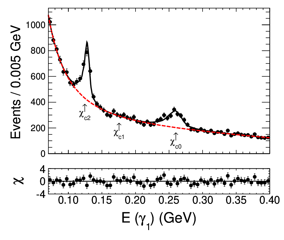
Electromagnetic showers are reconstructed from clusters of energy deposits in the EMC crystals. The energy deposited in nearby TOF counters is included to improve the reconstruction efficiency and energy resolution. Showers identified as photon candidates are required to satisfy fiducial and shower-quality criteria. A photon candidate is a shower detected in the EMC with a total energy deposit greater than 25 MeV and with an angle $\theta$ with respect to the $e^{+}$ beam direction in the range $|\cos\theta|<0.75$. This requirement is used to suppress continuum background $e^{+}e^{-}\rightarrow\gamma\gamma(\gamma)$, where the two energetic photons are mostly distributed in the forward and backward regions. We restrict the analysis to events that have no detected charged particles. The average event vertex of each run is assumed as the origin for the selected candidates. For $\psi^{\prime}\rightarrow\gamma_{1}\chi_{c0,2}$, $\chi_{c0,2}\rightarrow\gamma_{2}\gamma_{3}$ analysis, events are required to have three photon candidates, among which the smallest energy photon is selected as the radiated photon $\gamma_{1}$ and the second-largest and the largest energy photons are defined as $\gamma_{2}\gamma_{3}$ from $\chi_{c0,2}$ decays. An energy-momentum conservation constraint 4C-fit is performed, and events with $\chi^{2}\leq 80$ are retained in the final selection. The energy spectrum of the radiated photons is shown in Fig. 1, where enhancements due to the $\chi_{c0}$ and $\chi_{c2}$ over substantial backgrounds are clearly observed.

To determine signal efficiencies 100K signal MC event samples are generated for the $\chi_{c0}$ and the $\chi_{c2}$, with PDG values for the masses and widths [12]. The radiative transition $\psi(2S)\rightarrow\gamma_{1}\chi_{c0}$ is generated using a $(1+\mbox{cos}^{2}\theta)$ distribution, where $\theta$ is the radiative photon angle relative to the positron beam direction, in accordance with expectations for pure E1 transitions. The $\chi_{c0}\rightarrow\gamma_{2}\gamma_{3}$ decays are generated using a uniform angular distribution. Although the radiative transition $\psi(2S)\rightarrow\gamma_{1}\chi_{c2}$ is dominantly pure E1 [24, 25], there is some recent experimental evidence that the decay has contributions from higher-order multipoles [26]. The full angular amplitudes for $\psi^{\prime}\rightarrow\gamma_{1}\chi_{c2}$ are discussed in association with Eq. (5) in Section V. Furthermore, the $\gamma_{2}\gamma_{3}$ photons in the decay $\chi_{c2}\rightarrow\gamma_{2}\gamma_{3}$ are expected to be mostly in a pure helicity-two state; the ratio of the partial two-photon widths for the helicity-zero and helicity-two amplitudes is predicted to be less than 0.5% [5]. Thus the signal MC for the decay $\psi^{\prime}\rightarrow\gamma_{1}\chi_{c2}$, $\chi_{c2}\rightarrow\gamma_{2}\gamma_{3}$ is generated with $\gamma_{2}\gamma_{3}$ in a helicity-two state as described in Section V.

The energy resolutions determined by the MC simulations are $\sigma(E_{\gamma_{1}})=6.74\pm 0.29$ MeV for $\chi_{c0}$ and $\sigma(E_{\gamma_{1}})=3.91\pm 0.09$ MeV for $\chi_{c2}$. The efficiencies determined from MC simulations for the $\chi_{c0}$ and $\chi_{c2}$ are $\epsilon(\chi_{c0})=(35.4\pm 0.06)\%$ and $\epsilon(\chi_{c2})=(38.0\pm 0.07)\%$. The difference between $\epsilon(\chi_{c0})$ and $\epsilon(\chi_{c2})$ is due primarily to the different angular distributions.

The dominant non-peaking background that is apparent in the spectrum in Fig. 1 is from continuum $e^{+}e^{-}\rightarrow\gamma\gamma(\gamma)$ processes. It is determined from MC simulations that contributions to the background due to radiative decays to the $\eta$, $\eta^{\prime}$, and $3\gamma$ decays of $\psi^{\prime}$ are non-peaking, spread over the full range of $E_{\gamma_{1}}$, and negligible. Therefore, they do not change the shape of the dominant continuum background. In addition we use MC simulations to investigate possible sources of peaking backgrounds. These are found to come from $\chi_{c0,c2}\rightarrow\pi^{0}\pi^{0}$ and $\eta\eta$ decays and $\pi^{0}(\eta)\rightarrow\gamma\gamma$, where two of the $\gamma$s have low momentum and are not detected or are outside of the fiducial volume of this analysis. We generate at least 100K events of each type to determine the efficiencies for the peaking backgrounds, and use the efficiencies and branching fractions measured by BESIII [14] to determine the numbers of peaking background events listed in Table 1.

An unbinned maximum likelihood (ML) fit is done to the $E_{\gamma_{1}}$ spectrum as shown in Fig. 1. The shape of the large nonpeaking background in the spectrum is determined with the 44.1 pb^-1 of off-$\psi^{\prime}$ data taken at $\sqrt{s}=3.65$ GeV, as well as the $921.8$ pb^-1 of $\psi(3770)$ data taken at $\sqrt{s}=3.773$ GeV. As is evident in Fig. 2, the off-$\psi^{\prime}$ data are in good agreement with the high statistics $\psi(3770)$ data, for which transitions to either the $\chi_{c0}$ or $\chi_{c2}$ states are expected to be less than 8 events [12]. We also generate $e^{+}e^{-}\rightarrow\gamma\gamma(\gamma)$ MC events using the Babayaga QED event generator [27] and confirm that the shapes from the 3.65 GeV and 3.773 GeV samples are consistent with being due to the QED process. The $E_{\gamma_{1}}$ distribution for the $\psi(3770)$ data is fitted with the data-driven function:

where $p_{0}$, $p_{1}$, $p_{2}$ and $a$ are parameters which are obtained in a fit to the $\psi(3770)$ data in Fig. 2. In the nominal fit to the $\psi^{\prime}$ data, the background shape is fixed to Eq. (2), but its normalization is allowed to float. The shapes of the $\chi_{c0}$ and $\chi_{c2}$ resonances used in the fit are extracted from a nearly background-free $\psi^{\prime}\rightarrow\gamma_{1}\chi_{c0,2},\chi_{c0,2}\rightarrow K^{+}K^{-}$ sample shown in Fig. 3. The purity of the sample is larger than 99.2%. The shapes of the signal peaks in the $E{\gamma_{1}}$ spectrum are fixed to the smoothed-histograms of the $\psi^{\prime}\rightarrow\gamma_{1}\chi_{c0,2},\chi_{c0,2}\rightarrow K^{+}K^{-}$ sample, and the yields are allowed to float. The estimated numbers of peaking background events from $\chi_{c0,c2}\rightarrow\pi^{0}\pi^{0}$ and $\eta\eta$ that contribute to the $\chi_{c0}$ and $\chi_{c2}$ signals are 25.8 and 7.8 events, respectively, as listed in Table 1. They are subtracted from the fitted yields, and after this subtraction, the signal yields are $N(\chi_{c0})=813\pm 63$ and $N(\chi_{c2})=1131\pm 66$. The product branching fractions are determined from the relation

where $N_{\psi^{\prime}}$ is the total number of $\psi^{\prime}$ in the data sample. The measured product branching fractions are listed in Table 2. We use the PDG average values,

to determine $\mathcal{B}(\chi_{c0,2}\rightarrow\gamma\gamma)$, $\Gamma_{\gamma\gamma}(\chi_{c0,2})$ and $\mathcal{R}$. These are also listed in Table 2.

Several sources of systematic uncertainties in the measurement of the branching fractions are considered, including: uncertainties on the photon detection and reconstruction; the number of $\psi^{\prime}$ decays in the data sample; the kinematic fitting; the fitting procedure and peaking background subtraction. Table 3 lists a summary of all sources of systematic uncertainties. Most systematic uncertainties are determined from comparisons of special clean, high statistics samples with results from MC simulations.

The number of $\psi^{\prime}$ events, $N_{\psi^{\prime}}$ , used in this analysis is determined from the number of inclusive hadronic $\psi^{\prime}$ decays following the procedure described in detail in [14]. The result is $N_{\psi^{\prime}}=(1.06\pm 0.04)\times 10^{8}$, where the error is systematic.

Three photons in the final states include a soft photon $\gamma_{1}$ from the radiative transition and two energetic photons $\gamma_{2}\gamma_{3}$ from $\chi_{c0,2}$ decays. The photon detection efficiency and its uncertainty for low energy photons are studied using three different methods described in Ref. [28]. On average, the efficiency difference between data and MC simulation is less than 1% [28]. The momenta of the two energetic photons are more than 1.5 GeV/$c$. The systematic uncertainty due to the reconstruction of two energetic photons is determined to be 0.25% per photon as described in Ref. [29]. The total uncertainty associated with the reconstruction of the three photons is 1.5%.

The uncertainty due to the kinematic fit is estimated using a sample of $e^{+}e^{-}\rightarrow\gamma\gamma(\gamma)$, which has the same event topology as the signal. We select the sample by using off-$\psi^{\prime}$ data taken at $\sqrt{s}=3.65$ GeV to determine the efficiency difference between data and MC for the requirement of $\chi^{2}_{4C}<80$ in the 4C-fit. The uncertainty due to kinematic fitting determined in this way is 1%.

Since the signal shapes are obtained from $\psi^{\prime}\rightarrow\gamma\chi_{c0,2}$, $\chi_{c0,2}\rightarrow K^{+}K^{-}$ events in the data, the uncertainty due to the signal shape is negligible. The shape of the continuum background is parameterized using the data-driven function in Eq. (2); the parameters obtained in the fitting to off-$\psi^{\prime}$ data sample are fixed in the nominal fitting to $\psi^{\prime}$ data. The systematic uncertainty due to the choice of parametrization for the background shape is estimated by varying the fitting range and the order of polynomial in our data-driven function. We find relative changes on the $\chi_{c0}$ and $\chi_{c2}$ signal yields of 3.2% and 2.9%, respectively, which are taken as the uncertainties due to the resonance fitting.

The expected numbers of peaking background events from $\chi_{c1,2}\rightarrow\pi^{0}\pi^{0}$ and $\chi_{c0,2}\rightarrow\eta\eta$ decays summarized in Table 1 use BESIII measurements for $\mathcal{B}(\chi_{c1,2}\rightarrow\pi^{0}\pi^{0}/\eta\eta)$ [14]. The uncertainties on the $\pi^{0}\pi^{0}/\eta\eta$ contributions are estimated to be 0.3% and 0.1% for $\chi_{c0}$ and $\chi_{c2}$, respectively. The systematic uncertainties due to the trigger efficiency in these neutral channels are estimated to be $<0.1$%, based on cross-checks using different trigger conditions [14, 30]. We have assumed pure helicity-two decay of $\chi_{c2}\rightarrow\gamma\gamma$. In a relativistic calculation, Barnes [5] predicted the helicity-zero component to be 0.5%. In section V, the ratio of the two photon widths for the helicity-zero and helicity-two amplitudes is measured to be $0.00\pm 0.02\pm 0.02$. To be conservative, we determine the change in our $\chi_{c2}$ result when a helicity-zero component of 3% is included, corresponding to an upper limit at 90% confidence level from the measurement in this paper, to be 0.4%, and use that as the helicity-state-associated systematic error.

All sources of systematic errors are listed in Table 3. We assume that all systematical uncertainties are independent and add them in quadrature to obtain the total systematical uncertainty. For the measurements of $\mathcal{B}(\chi_{c0,2}\rightarrow\gamma\gamma)$, the uncertainty due to the $\psi^{\prime}\rightarrow\gamma\chi_{c0,2}$ branching fractions is kept separate and quoted as a second systematic uncertainty.

In $\chi_{c2}\rightarrow\gamma\gamma$ decay, the final state is a superposition of helicity-zero ($\lambda=0$) and helicity-two ($\lambda=2$) components, where $\lambda$ is the difference in the helicity values of the two photons. The formulae for the helicity amplitudes in $\psi^{\prime}\rightarrow\gamma\chi_{c2},\chi_{c2}\rightarrow\gamma\gamma$, which include higher-order multipole amplitudes, are:

where $x=\mathnormal{A}_{1}/\mathnormal{A}_{0}$, $y=\mathnormal{A}_{2}/\mathnormal{A}_{0}$, and $\mathnormal{A}_{0,1,2}$ are the $\chi_{c2}$ helicity 0, 1, 2 amplitudes, respectively, $\theta_{1}$ is the polar angle of the radiative photon, where the electron beam is defined as the $z$ axis in the $e^{+}e^{-}$ center-of-mass frame, and $\theta_{2}$ and $\phi_{2}$ are the polar angle and azimuthal angle of one of the photons from $\chi_{c2}$ decay in the $\chi_{c2}$ rest frame, relative to the radiative photon direction as polar axis; $\phi_{2}=0$ is defined by the electron beam direction. The factor $f_{0/2}=|F_{0}|^{2}/|F_{2}|^{2}=\Gamma^{\lambda=0}_{\gamma\gamma}(\chi_{c2})/\Gamma^{\lambda=2}_{\gamma\gamma}(\chi_{c2})$ is the ratio of partial two-photon widths for the helicity-zero and helicity-two components, where $F_{0}$ ($F_{2}$) is the helicity-zero (two) amplitude in the decay $\chi_{c2}\rightarrow\gamma\gamma$. Further information on the formulae for the helicity amplitudes can be found in Ref. [31].

An unbinned ML fit to the angular distribution is performed to determine $x$, $y$ and $f_{0/2}$ values. We define twelve factors [26]:

The mean values of $a_{1},\cdots,a_{12}$ can be determined with $\psi^{\prime}\rightarrow\gamma\chi_{c2}$, $\chi_{c2}\rightarrow\gamma\gamma$ MC events, where phase space is used for the simulation of all the angular distributions:

where $N$ is the number of events after all selections from phase space MC samples. Since $\bar{a}_{n}$ is calculated with phase space MC events after selection, it naturally accounts for the detector acceptance effects.

The normalized probability-density function is written as:

A total log-likelihood function is constructed as: $\ln\mathcal{L}=\sum_{i=1}^{n}\ln f_{i}(x,y,f_{0/2})$, where the sum is over all the events in the signal region (here the signal region is defined as $0.09<E_{\gamma_{1}}<0.15$ GeV). The log-likelihood function for the signal is given by $\ln\mathcal{L}_{s}=\ln\mathcal{L}-\ln\mathcal{L}_{b}$, in which $\ln\mathcal{L}_{b}$ is the normalized sum of logarithmic likelihood values from background events and is calculated using the events in the sidebands, which are defined in the ranges $(0.07,0.08)$ GeV (lower sideband) and $(0.16,0.20)$ GeV (higher sideband) in the the $E_{\gamma_{1}}$ spectrum. By maximizing the logarithm of the likelihood function $\ln\mathcal{L}_{s}$, the best values of $x$, $y$ and $f_{0/2}$ are determined. Before fitting to the data, input and output checks were done using MC samples, and the results used to validate the fitting procedure.

BESIII has determined $x$ and $y$ to be $x=1.55\pm 0.05(\mbox{stat.})\pm 0.07(\mbox{syst.})$ and $y=2.10\pm(\mbox{stat.})0.07\pm 0.05(\mbox{syst.})$ [26] using the decays $\psi^{\prime}\rightarrow\gamma\chi_{c2}$, $\chi_{c2}\rightarrow\pi^{+}\pi^{-}/K^{+}K^{-}$. Therefore, in the nominal fit, the $x$ and $y$ parameters are fixed to the measured values, and the remaining parameter $f_{0/2}$ is determined to be:

where the error is statistical. Figure 4 shows the angular distributions of background-subtracted data and the fitted results for $\chi_{c2}\rightarrow\gamma\gamma$ events. It is found that all angular distributions are consistent with the fitted results within errors. As mentioned in Section IV, for the measurements of the branching fractions we use the formulae in Eq. (5) to generate MC events for efficiency determination of $\psi^{\prime}\rightarrow\gamma\chi_{c2}$, $\chi_{c2}\rightarrow\gamma\gamma$ decay, with the $x$, $y$ and $f_{0/2}$ parameters fixed at their measured central values ($x=1.55$, $y=2.10$ and $f_{0/2}=0.0$).

In order to test the reliability of the fit, we allow the $x$ and $y$ parameters to float in the fit, in which case the likelihood fit to data yields

where the errors are statistical. The results are consistent with the previous BESIII measurements of the $\psi^{\prime}\rightarrow\gamma\chi_{c2}$, $\chi_{c2}\rightarrow\pi^{+}\pi^{-}/K^{+}K^{-}$ decays [26].

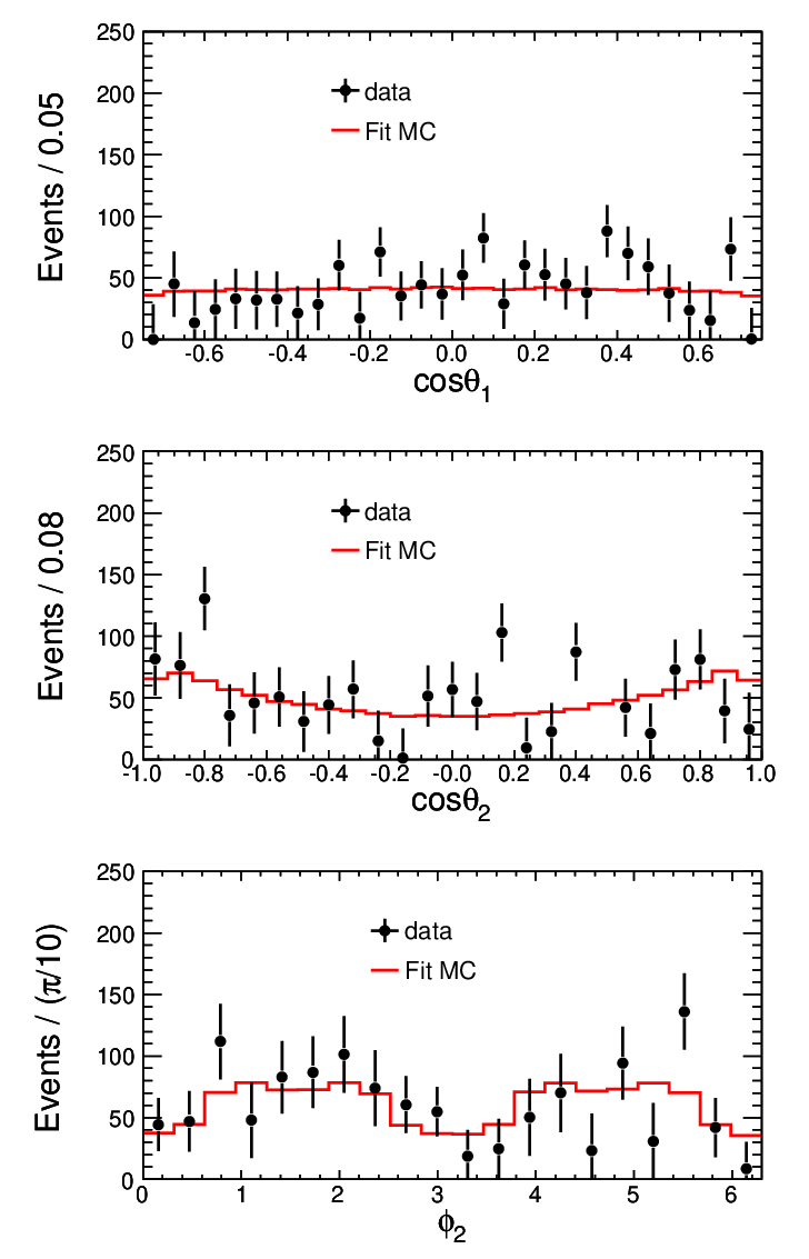
The goodness of the fit is estimated using Pearson^′s $\chi^{2}$ test  [32]. The data and MC are divided into 6 bins of equal width in each dimension (i.e. $\cos\theta_{1}$, $\cos\theta_{2}$, $\phi_{2}$) of the three-dimension angular distribution. The numbers of events in each cell for data and the normalized MC sample are compared. The $\chi^{2}$ is defined as:

where $n^{DT}_{i}$ ($\sigma_{n^{DT}_{i}}$) is the observed number (its error) of signal events after background subtraction in the $i$th bin from data and $n^{MC}_{i}$ is the expected number of events predicted from MC in the $i$th bin using $f_{0/2}$ fixed to the value determined in the analysis. If the number of events in a bin is less than 5, we add the events to the adjacent bin. The result of the $\chi^{2}$ test of the fitting is: $\chi^{2}/n.d.f=87.3/88=0.99$, where $n.d.f.$ is the number of degrees of freedom. The result shows that the fit quality is acceptable.

Since $f_{0/2}$ is a ratio, many systematic errors cancel, and only the effects due to MC simulation of detector response, the uncertainties on the measured $x$ and $y$ parameters, background substraction, $\chi_{c0}$ contamination are considered here. Among these sources of the systematic uncertainties, the MC simulation of detector response is dominant; the others are tiny and are neglected.

As discussed above, the $x$ and $y$ parameters are fixed to the measured values from Ref. [26] in the ML fit to $\chi_{c2}\rightarrow\gamma\gamma$ events in order to obtain the ratio $f_{0/2}$. In the fit we change the $x$ and $y$ central values by one standard deviation of the measured values [26], and find that the effect on $f_{0/2}$ is negligible. To estimate the uncertainty due to background subtraction, we vary the sideband region from $(0.07,0.08)$ GeV (lower sideband) and $(0.16,0.20)$ GeV (higher sideband) to $(0.07,0.09)$ GeV and $(0.15,0.20)$ GeV. After subtraction of the background based on the sum of recalculated logarithmic likelihood values, $\ln\mathcal{L}_{b}$, we find that the fitted $f_{0/2}$ value is almost unchanged. From MC simulation, 0.028% of the $\chi_{c0}\rightarrow\gamma\gamma$ events are distributed under the $\chi_{c2}$ signal region; the uncertainty due to $\chi_{c0}$ contamination is estimated to be negligible.

The uncertainty due to the inconsistency between data and MC simulation on the angular distributions for $\chi_{c2}$ events can be tested using $\chi_{c0}$ events. Since the $\chi_{c0}$ is pure helicity-zero, the $x$ and $y$ parameters are expected to be zero. In $\chi_{c0}\rightarrow\gamma\gamma$ decay, the difference of helicity values of the two photons is also expected to be zero, so only the helicity-zero term in Eq. (5) remains, which modifies Eq. (5) to:

where the product factor $f_{0/2}$ is moved to the front factor of the helicity-two term and renamed as $f_{2/0}$, and the $(3\cos^{2}\theta_{2}-1)^{2}$ term associated with $\lambda=0$ amplitude in Eq. (5) is replaced by 1, so that one can obtain the expected angular distribution $W_{0}=1+\cos^{2}\theta_{1}$ from Eq. (23) if the parameters $x=0$, $y=0$ and $f_{2/0}=0$, as expected. Therefore, we fit the angular distribution of $\chi_{c0}$ with the Eq. (23) using the same method as in $\chi_{c2}$ decays; non-zero $x$, $y$ and $f_{2/0}$ values will indicate the inconsistency between data and MC simulation. The systematic error is taken as the shift from 0 plus its error. The fitted results are $x=-0.11\pm 0.09$, $y=0.13\pm 0.07$ and $f_{2/0}=0.00\pm 0.02$. The correlation coefficient between $x$ and $y$ is -0.27, while it is 0.0 between $x$ ($y$) and $f_{2/0}$. Thus we take 0.02 as the systematic error for the measurement of $f_{0/2}$ in the fit to $\chi_{c2}$ events. Studies with MC simulated data samples demonstrate that a systematic error in modeling the $\theta_{1}$, $\theta_{2}$, and $\phi_{2}$ efficiency produces a shift of approximately the same size for $f_{2/0}$ in $\chi_{c0}$ sample and $f_{0/2}$ in $\chi_{c2}$ sample, when the latter sample is generated with $x=1.55$, $y=2.10$ and $f_{0/2}=0$. Therefore, we assume the observed shift from $f_{2/0}$ for the true $\chi_{c0}$ data is an estimate of the systematic error on the measured values of $f_{0/2}$ for the two-photon decay of $\chi_{c2}$.

References

- [1] H. W. Huang, C. F. Qiao, and K. T. Chao Phys. Rev. D 54,2123(1996); C. W. Hwang and R. S. Guo, Phys. Rev. D 82, 034021 (2010).
- [2] R. Barbier, R. Gatto, and R.Kgerler, Phys. Lett. B 60,183(1976).
- [3] L. Laudau, Phys. Abstr. A 52,125(1949); C. N. Yang, Phys. Rev. 77,242(1950).
- [4] T. Appelquist and H. D. Politzer, Phys. Rev. Lett. 34, 43 (1975).
- [5] T. Barnes, Proceedings of the IX International Workshop on Photon-Photon Collisions edited by D. O. Caldwell and H. P. Paar (World Scientific, Singapore, 1992), p. 263.
- [6] S. N. Gupta, J. M. Johnson, and W. W. Repko, Phys. Rev. D 54, 2075 (1996).
- [7] D. Ebert, R. N. Faustov, and V. O. Galkin, Mod. Phys. Lett. A 18, 601 (2003); Phys. Rev. D 67, 014027 (2003).
- [8] S. Godfrey and N. Isgur, Phys. Rev. D 32, 189 (1985).
- [9] G. A. Schuler, F. A. Berends, and R. van Gulik, Nucl. Phys. B 523, 423 (1998).
- [10] J. P. Lansberg and T. N. Pham, Phys. Rev. D 79, 094016 (2009).
- [11] J. J. Dudek and R. G. Edwards, Phys. Rev. Lett. 97, 172001 (2006).
- [12] K. Nakamura et al. (Particle Data Group), J. Phys. G 37, 075021 (2010) and 2011 partial update for the 2012 edition.
- [13] K. M. Ecklund, et al. (CLEO Collaboration), Phys. Rev. D 78,091501(R) (2008).
- [14] M. Ablikim et al. (BES Collaboration), Phys. Rev. D 81, 052005 (2010).
- [15] M. Ablikim et al. (BES Collaboration), Nucl. Instrum. Meth. A 614, 345 (2010).
- [16] J. Z. Bai et al. (BES Collaboration), Nucl. Instrum. Meth. A 344, 319 (1994); J. Z. Bai et al. (BES Collaboration), Nucl. Instrum. Meth. A 627, 319 (2001).
- [17] J. Z. Bai et al. (BES Collaboration), Nucl. Instrum. Methods Phys. Res., Sect. A 344, 319 (1994); 458, 627 (2001).
- [18] Special issue on Physics at BESIII, edited by K. T. Chao and Y. F. Wang, Int. J. Mod. Phys. A 24, Supp. (2009).
- [19] S. Agostinelli et al. (geant4 Collaboration), Nucl. Instrum. Meth. A 506, 250 (2003).
- [20] S. Jadach, B. F. L. Ward and Z. Was, Comput. Phys. Commun. 130, 260 (2000); S. Jadach, B. F. L. Ward and Z. Was Phys. Rev. D 63, 113009 (2001).
- [21] D. J. Lange et al., Nucl. Instrum. Meth. A 462, 1 (2001).
- [22] J. C. Chen, G. S. Huang, X. R. Qi, D. H. Zhang, and Y. S. Zhu, Phys. Rev. D 62, 034003 (2000).
- [23] W. D. Li, H. M. Liu et al., in Proceedings of CHEP06, Mumbai, India, 2006 edited by Sunanda Banerjee (Tata Institute of Fundamental Research , Mumbai, 2006).
- [24] M. Oreglia et al. (Crystal Ball Collaboration), Phys. Rev. D 25, 2259 (1982).
- [25] M. Ambrogiani et al. (E835 Collaboration), Phys. Rev. D 65, 052002 (2002).
- [26] M. Ablikim et al. (BES Collaboration), Phys. Rev. D 84, 092006 (2011).
- [27] C. M. Carloni Calame et al., Nucl. Phys. Proc. Suppl. 131, 48 (2004), and references therein.
- [28] M. Ablikim et al. (BES Collaboration), Phys. Rev. D 83, 112005 (2011).
- [29] M. Ablikim et al. (BES Collaboration),Phys. Rev. Lett. 105, 261801 (2010).
- [30] N. Berger, K. Zhu et al., Chinese Physics C 34, 1779 (2010)
- [31] T. Luo, G. Li, H. B. Li, Z. H. Yu, The deduction of the angular distribution of , in preparation.
- [32] W. Eadie et al., Statistical Methods in Experimental Physics (North-Holland Publishing Company, Amsterdam-London, 1971).
- [33] M. B. Voloshin, Prog. Part. Nucl. Phys. 61, 2, 455 (2008).