The Gröbner stratification of a tropical variety
Abstract.
Each Gröbner stratum of a tropical variety is a connected set of points, all of which induce the same initial subscheme. The Gröbner stratification is a coarsening of the decomposition into Gröbner polyhedra, and has the advantage that it does not depend on a choice of compactification. We give an example of a curve over a field with non-trivial valuation whose Gröbner stratification is strictly finer than the coarsest polyhedral decomposition of the tropical variety. We also show that the Gröbner stratification of a locally matroidal tropical variety is completely determined by the underlying tropical variety.
Let be a field with valuation and let be the image of its valuation. We assume and fix a splitting of the valuation, which is guaranteed to exist if is algebraically closed or if is discrete. For any closed subscheme and any point of , it is possible to take its weighted initial scheme (see Definition 1). The tropicalization is the set of all weights such that is non-empty. There exists a polyhedral complex whose support is , but the polyhedral structure is not unique, and there may not be a coarsest polyhedral structure [ST08, Example 5.2]. In particular, the construction of the polyhedral complex depends on the choice of a compactification in which we take to be the closure of . Then each polyhedron of the Gröbner complex is the closure of the set of such that is some fixed scheme.
Without choosing a compactification, we can stratify the tropical variety based on the initial ideal , taken within the torus . More precisely, a stratum of the Gröbner stratification is a component of the set of points such that is some fixed subscheme. Unlike the Gröbner complex, each stratum need not be the relative interior of a convex polyhedron, nor even contractible (for example, take two tropical planes meeting in a single point), but it is at least an open subset of an affine linear subspace of .
The purpose of this paper is to contrast the Gröbner stratification with topological stratification, which depends solely on as a subset of , and is defined to be the finest stratification which is compatible with local products in the tropical variety. More precisely, suppose that we have a linear isomorphism and an open set such that factors as a product of a subset of with an open subset . The topological stratification is defined to be the finest stratification such that for any local factoring of an open set , each stratum also factors as the product of a subset of with . Unlike the Gröbner stratification, the topological stratification depends only on and not on itself. Without using this terminology, Sturmfels and Tevelev gave a recipe for constructing a tropical variety whose Gröbner stratification is strictly finer than its topological stratification [ST08, Example 3.10]. We give an explicit such example as a curve over a field with non-trivial valuation in Section 1, and we examine the preimages of its Gröbner strata in the Berkovich skeleton.
The Berkovich analytification maps surjectively onto by taking the valuations of the coordinate functions. When is a curve, contains a distinguished graph, the skeleton, coming from a minimal semistable reduction of , and is the image of the skeleton under a map which is linear on each edge. Thus, there are finitely many points in which are the images of the vertices of the skeleton. Any point whose neighborhood in is not a union of open segments must be a zero-dimensional Gröbner stratum and also the image of a vertex of the skeleton. Nonetheless, in general, the set of images of vertices of the skeleton neither contains nor is contained in the set of zero-dimensional Gröbner strata. Example 2.6 of [BPR11] is a curve whose skeleton has a vertex which maps to a point in the interior of a one-dimensional Gröbner stratum. On the other hand, our example in Section 1 has a zero-dimensional Gröbner stratum contained in an open half-ray, whose preimage in the skeleton is two disjoint edges.
Our detailed examination of this example occupies the entirety of Section 1. In Section 2, we compare the two strata on general tropical varieties. Proposition 6 implies that in any case where the Gröbner refines the tropical stratification, the corresponding initial ideals will have the same support, but different non-reduced structures. We prove that the two strata agree for locally matroidal tropical varieties and for curves whose multiplicities are all one (Theorem 8 and Corollary 9). Throughout the paper, will denote the valuation ring of with maximal ideal and residue field .
Acknowledgments
I have been supported by the National Science Foundation under award DMS-1103856. I would like to thank Sam Payne for many helpful suggestions, including the question which prompted this paper. Walter Gubler pointed me towards Example 3.10 in [ST08]. I also thank the Institut Mittag-Leffler and the Max Planck Institute in Bonn for their hospitality during my work on this paper.
1. A non-trivial Gröbner stratification
In this section, we give an example of a curve whose tropicalization has an open ray, which contains 3 distinct Gröbner strata. First, it will be useful to define the initial degeneration in greater generality than has appeared in the literature. In particular, the following does not require the entries of to be in the value group.
Definition 1.
For any , we let denote the -subalgebra of generated by all terms such that , where is the vector of exponents. We define to be the closure of in . We then define a ring homomorphism by sending the monomial to
where denotes the image of in the residue field . The initial degeneration is defined to be , where is the map of schemes induced by .
If the entries of lie in the value group, then induces an isomorphism from to the special fiber of , and if not, can be thought of as the special fiber of after extending to a field whose valuation group contains the coordinates of .
For our example, we let be an element with non-trivial valuation, and for convenience, we rescale the valuation such that . Throughout this section, will denote the ideal generated by the minors of the matrix
| (1) |
and will be the subvariety of defined by . Abstractly, is isomorphic to with a finite number of points removed, and it can be given explicitly as the image of the rational map
We will use , , and as coordinates for . The intersection of the tropical variety of with the half space defined by is the single half ray with . The initial stratification divides this half-ray into three strata, based on the ideal defining :
| (2) |
Note that all three of these initial schemes have the same support, namely the subtorus defined by , but different non-reduced structures.
| Component | ||
|---|---|---|
We now compute the skeleton of and show that the map from this skeleton to does not distinguish from nearby points. We will assume that is algebraically closed and that does not have characteristic or . The purpose of these two assumptions is so that the boundary consists of exactly distinct closed points which are the roots of the polynomials shown in the first column of Table 1. In characteristics and , there are extra coincidences among the divisors in Table 1, which change the skeleton, but not the part mapped to the half-space . There is a unique -model of defined by taking to be a non-constant rational function on the special fiber. This model is not semistable because each root of intersects a corresponding root of in the special fiber. If we blow up the special fiber at each of the three roots of , we obtain a semistable model whose special fiber has components. The original component maps to . The exceptional divisor of the blow-up at maps to and the other two exceptional divisors map to . The dual graph of the special fiber is a claw graph and the Berkovich skeleton consists of this graph together with infinite edges. The map of the Berkovich skeleton to is shown in Figure 1.
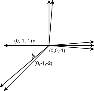
The preimage of the half-plane in the skeleton consists of two disjoint rays. Since has a deformation retract onto its skeleton, this implies that itself decomposes into two connected components in the corresponding analytic domain defined by . We now compute this decomposition explicitly. Since is generated by all minors of (1), it also contains the determinant
This is the equation of the projection of onto the and coordinates. We now assume that does not have characteristic in order to use the quadratic formula to find analytic representations of the two branches of in terms of :
| (3) |
which can be expanded as a power series in , convergent on the analytic disk defined by . Using the left-most minor of (1), we have
and we can use the expansion of (3) as a power series to get analytic formulas:
| (4) |
for the positive and negative branch of respectively. Thus, (3) and (4) give equations for each branch of as the graph of an analytic function from the coordinate to the and coordinates. Although we only defined for subschemes of the torus, we can also take initial ideals in the analytic domain . For and , the formulas (3) and (4) give . Thus, either branch on its own degenerates to the subtorus defined by , and it is only when the two branches degenerate together that the “twisted” non-reduced structure appears in (2).
An important use of the polyhedral complex decomposition of a tropical variety is the theory of tropical compactifications, as introduced by Tevelev [Tev07] and later extended to fields with non-trivial valuation by Qu [Qu09] (see also [LQ11]) and Gubler [Gub11, Sec. 11]. The topological stratification of has polyhedral strata, and we can compactify by taking its closure inside the corresponding toric scheme. This compactification cannot be a tropical compactification since a tropical compactification must come from a polyhedral complex which refines the Gröbner stratification [Gub11, Cor. 12.9]. We examine this compactification explicitly.
A toric scheme over corresponds to a fan in [Gub11, Sec. 7], and we will look at one affine chart of the scheme coming from the cone over the topological stratification of , placed at height . Our usual ray of produces the cone generated by the vectors and . The corresponding affine toric scheme is , where the subtorus is defined by . Near the point in the special fiber defined by and , the closure of has two branches, given by substituting into the analytic equations (3) and (4).
Thus, consists of two analytic branches, each isomorphic to the completion of the two-dimensional scheme , meeting at the single closed point . This is a textbook example of a non-Cohen-Macaulay singularity, which was the ingredient suggested in [ST08, Ex. 5.2] for building a tropical variety with a polyhedral structure which is too coarse to be tropical. As they argued, the non-Cohen-Macaulay point, together with Theorem 1.2 of[Tev07] give another proof that this (partial) compactification is not tropical.
2. Locally matroidal tropical varieties
In this section, we more systematically compare the Gröbner and topological stratifications. Proposition 6 relates the topological stratification to the structure of the initial ideals. The main result of this section is Theorem 8, which gives criterion for the two stratifications to agree.
We first need several lemmas, which extend standard results to initial ideals at points whose coordinates are not necessarily in the value group. In particular, Lemma 3 tells us that even when is not the special fiber of , it can be realized as the special fiber of a flat family over some extension of .
Lemma 2.
Let be an extension of valued fields and any point in . Then as subschemes of the torus, where is the residue field of .
Proof.
We let be the closure of the extension in the tilted torus , as in Definition 1. We have a commutative diagram:
where and are as in Definition 1. By [OP10, Thm. A.3], the ideal of is the image of the ideal of under the inclusion on the left (although [OP10] assumes that is algebraically closed, this isn’t used in the proof of Theorem A.3). Thus, the ideal of is the image of the ideal of by the upper-left path around the square. The ideal of is the image by the lower right path, and so the two schemes are equal. ∎
Lemma 3.
Let be a point in . Then there exists a valuation ring dominating and a flat family over whose special fiber is isomorphic to and whose general fiber is , where is the fraction field of .
Proof.
We build the extension , together with a splitting of its valuation homomorphism one coordinate of at a time. Let and equal and respectively, and we inductively define as follows. If no multiple of lies in , then we take to be the transcendental extension with the unique extension of the valuation given by . Otherwise, if is in , with minimal, then is constructed as the extension , where is a primitive th root of . In both cases, we also extend the splitting, which by abuse of notation, we still call , by setting . In the end, we have produced a valued field whose value group includes the entries of . We also note that at each stage of our construction of , the residue field of the valuation ring is unchanged.
The desired family will be , which is flat and finite presentation over [OP10, Prop. A.1]. By Lemma 2, we know that is , and so it only remains to show that the map as in Definition 1 induces an isomorphism between and the special fiber of . First, since , each variable of is the image of under , so is surjective. Second, for any monomial in the kernel of , i.e. with , then is in , so there exists , with . Thus, , and with positive valuation, so vanishes on the special fiber. We’ve shown that the special fiber of is , so forms the desired family. ∎
Lemma 4.
Let be a point in . Then for sufficiently small vectors , , where the last initial ideal is taken with respect to the trivial valuation on .
Proof.
By choosing a compactification into , we can partition into a Gröbner complex as in [Gub11, Sec. 10]. Now we claim that the lemma is true if we take sufficiently small such that any polyhedron containing also contains . If so, we can choose an extension whose valuation group contains the coordinates of and as in the proof of Lemma 3. Then Proposition 10.9 of [Gub11] tells us that , and Lemma 2 tells us that the same equality holds over . ∎
Proposition 5.
A point is in a Gröbner stratum of dimension if and only if the maximal subtorus preserving has dimension .
Proof.
For sufficiently small vectors , the initial degeneration equals the initial degeneration by Lemma 4. Therefore, lies in a -dimensional Gröbner stratum if and only if is equal to for all in a -dimensional vector space. The scheme is unchanged by taking initial with respect to some rational weight vector if and only if is invariant under the action of the corresponding one-dimensional subtorus of . Thus, the vector space of all weights under which is unchanged corresponds to the maximal subtorus under which is invariant, and in particular, they have the same dimension. ∎
The proof of Proposition 5 already shows that the Gröbner stratification refines the topological one. However, it can also be seen through the following characterization of the topological stratification in terms of initial ideals.
Proposition 6.
A point is in the topological stratum of dimension if and only if the maximal subtorus preserving the reduced subscheme of has dimension .
Proof.
First, let denote the reduced induced subscheme of and suppose that is preserved by some -dimensional subtorus, and thus the tropical variety of is a product with the vector space corresponding to the subtorus. Since taking reduced subschemes does not change the underlying set of a tropical variety, the tropical variety of now has the same property. Thus, is also a product with a vector space in a neighborhood of by Lemma 4, so is in an -dimensional topological stratum
Conversely, suppose that is a product with a -dimensional linear space in a neighborhood of . Then is globally a product with a vector space, and we can change coordinates to assume that the vector space generated by the first coordinate vectors. If we let be the projection of onto the last coordinates, then is the projection of the onto the last coordinates. Therefore, the Bieri-Groves theorem tells us that has dimension , where is the dimension of . For any irreducible component of , the projection must have dimension at most , so has dimension at most . However, is a -dimensional variety and is contained in , so they must be equal. Therefore, is invariant under the subtorus which acts on the first coordinates, as is the reduced subscheme of . ∎
Corollary 7.
If is a linear space in a neighborhood of a point , then the support of is a finite union of torus orbits.
Recall that at a point in the interior of a maximal cone of the Gröbner complex, the multiplicity is the sum of the multiplicities of all primary components of . By the balancing condition, the multiplicities in any neighborhood of a locally linear point will all be equal. However, we can given an intrinsic definition of the multiplicity at any locally linear point as the sum
where is the set of irreducible components of , and is the field of rational functions on which are invariant under the maximal subtorus of which preserves .
The tropicalizations of linear spaces have a purely combinatorial description in terms of the associated matroid [AK06], which we recall here. Let be a matroid with ground set and bases . For any basis and , let be the sum . Let be the set of bases for which is minimized, and it can be shown that is also the set of bases of a matroid. The Bergman fan of is the set of vectors for which has no loops. We say that a tropical variety is locally matroidal at a point if there exists a neighborhood of in which all multiplicities are and which is equal to a neighborhood of the Bergman fan of some matroid , possibly after a change of coordinates from an element of . Locally matroidal fans have been studied before as analogues of smooth varieties, for example in [Sha10] and [KS10, Sec. 7].
Theorem 8.
Let be locally matroidal point of . Then, in appropriate coordinates, is a linear subspace of . In particular, the Gröbner stratification and the topological stratification agree in a neighborhood of .
Corollary 9.
If is a curve and all multiplicities of are , then the Gröbner and topological stratifications on coincide.
Proof.
Since the Gröbner stratification refines the topological stratification, it suffices to prove that each one-dimensional topological stratum of is also a Gröbner stratum. However, any one-dimensional topological stratum is locally linear by definition, and thus matroidal, so the claim follows from Theorem 8. ∎
Recall that a subvariety of a torus is called schön if the initial degeneration is smooth for every
Corollary 10.
If is locally matroidal at all points , then is schön.
One ingredient in the proof of Theorem 8 is the fact that linear spaces are characterized by their tropicalizations, which was proved by Katz and Payne [KP11, Prop. 4.2]. Given this characterization, the remaining difficulty is to prove that the is reduced, for which we use the following.
Theorem 11.
If is generically reduced and its reduced induced subscheme is geometrically integral and normal, then is reduced.
Theorem 11 is a generalization of a result first obtained by Hironaka for degenerations over the localization of a ring of finite type over a field [Hir58, Lemma 4] (see also [Har77, Lemma III.9.12]). We use the Hironaka’s argument for the case when is an excellent DVR, and use Noetherian approximation to reduce to this case when is a general rank valuation.
Proof of Theorem 11.
Using Lemma 3, we let denote the coordinate ring of the flat family over the valuation ring, for which we drop the tilde and write . We let denote the unique minimal prime of .
We first prove the theorem under the assumption that is an excellent discrete valuation ring and write to denote a uniformizer of . We’ve assumed that is generically reduced, so generates the maximal ideal in , meaning that is a discrete valuation ring. Therefore, , the normalization of is a subring of , and so is a subring . However, is the field of fractions of , which we’ve assumed to be normal, so must equal .
Since is generically reduced, it will be sufficient to show that it has no embedded primes. Suppose that is any prime containing and we will show that is not an embedded prime of . Since is excellent, then, in particular, the normalization is a finite -module. We’ve shown that equals , so Nakayama’s Lemma implies that equals . In other words, is normal. Thus, the principal ideal in generated by cannot have any embedded primes, and thus cannot be an embedded prime of . This completes the proof when is an excellent DVR.
Now, we allow to be an arbitrary valuation ring and we reduce to the excellent case by Noetherian approximation. By [Gro66, Cor. 11.2.7], there exists a finite type -algebra , contained in , and a finite type, flat -algebra such that and as -algebras. Set to be the localization and let be its maximal ideal. By [Gro61, Prop. 7.1.7], there exists a discrete valuation ring dominating with the same field of fractions. From the proof of that proposition, we see that is the normalization of a localization of a ring of finite type over , so is excellent [Gro65, Schol. 7.8.3(iii)]. These various bases are summarized in the following commutative diagram:
| (5) |
We will write as for .
The rings in the bottom row of (5) are local rings and we now wish to the corresponding special fibers of the rings in the top row. The inclusions of into and are local homomorphisms, so if we take the quotients of the rings in (5) by the maximal ideals in the bottom row, we get a commutative diagram whose squares are tensor products:
By hypothesis, has a unique minimal prime. Thus, the only minimal prime of is the contraction [Gro65, Prop. 4.2.7(i)], and we will call this prime . Moreover, localizing at this prime kills off any embedded components in , so the localization of at is a subring of an integral domain and thus is generically reduced. Since is geometrically integral, then is integral and is the unique minimal prime over . Therefore, we can apply the proof of the excellent case to conclude that is radical. Since has no embedded primes, then neither do and [Gro65, Prop. 4.2.7(i)], which is what we wanted to prove. ∎
Proof of Theorem 8.
The degeneration and its reduced subscheme have the same tropicalizations as sets. In general, the tropicalization of the reduced subscheme could have lower multiplicities, but the fact that all the multiplicities are means that and its reduced subscheme have the same multiplicities as well. Therefore, the reduced subscheme of is isomorphic to the complement of a hyperplane arrangement in projective space [KP11, Prop. 4.2], and in particular it is normal. Thus, Theorem 11 implies that is reduced. The initial degenerations of a linear space are also linear spaces, so by Lemma 4, the initial subschemes are also reduced sufficiently close to . Therefore, the criteria in Propositions 5 and 6 agree, so the Gröbner and topological stratifications agree in this neighborhood. ∎
References
- [AK06] F. Ardila, C. Klivans: The Bergman complex of a matroid and phylogenetic trees, J. Combin. Theory Ser. B 96:1 (2006) 38–49.
- [BPR11] M. Baker, S. Payne, J. Rabinoff: Nonarchimedean geometry, tropicalization, and metrics on curves, preprint, arXiv:1104.0320.
- [Gro61] A. Grothendieck: Éléments de géometrétrie algébrique: II. Étude globale élémentaire de quelques classes de morphismes, Publ. Math. de l’IHÉS 8 (1961).
- [Gro65] A. Grothendieck: Éléments de géometrétrie algébrique: IV. Étude locale des schémas et des morphismes de schémas, Seconde partie, Publ. Math. de l’IHÉS 24 (1965).
- [Gro66] A. Grothendieck: Éléments de géometrétrie algébrique: IV. Étude locale des schémas et des morphismes de schémas, Troisième partie, Publ. Math. de l’IHÉS 28 (1966).
- [Gub11] W. Gubler: A guide to tropicalizations, preprint, arXiv:1108.6126.
- [Har77] R. Hartshorne: Algebraic Geometry, Graduate Texts in Mathematics 52, Springer, New York, 1977.
- [Hir58] H. Hironaka: A note on algebraic geometry over ground rings: the invariance of Hilbert characteristic functions under the specialization process, Illinois J. Math. 2:3 (1958) 355-366.
- [KP11] E. Katz, S. Payne: Realization spaces for tropical fans, Combinatorial aspects of commutative algebra and algebraic geometry, Abel Symp. 6 (2011) 73–88.
- [KS10] E. Katz, A. Stapledon: Tropical geometry and the motivic nearby fiber, Compositio Math., to appear. arXiv:1007.0511
- [LQ11] M. Luxton, Z. Qu: Some results on tropical compactifications, Trans. Amer. Math. Soc. 363:9 (2011) 4853–4876.
- [OP10] B. Osserman, S. Payne: Lifting tropical intersections, preprint, arXiv:1007.1314.
- [Qu09] Z. Qu: Toric schemes over a discrete valuation ring and tropical compactifications. PhD thesis, University of Texas at Austin (2009).
- [ST08] B. Sturmfels, J. Tevelev: Elimination theory for tropical varieties, Mathematical Research Letters 15:3 (2008) 534–562.
- [Sha10] K.M. Shaw: A tropical intersection product in matroidal fans, preprint, arXiv:1010.3967.
- [Tev07] J. Tevelev: Compactifications of subvarieties of tori, Am. J. Math. 129: 4 (2007) 1087–1104.