Universal Aspects of QCD-like Theories
Note: For “Physics at all scales: The Renormalization
Group,”
The Schladming Winter School on Theoretical
Physics.
Abstract
In these lectures I review some basic examples of how the concepts of universality and scaling can be used to study aspects of the chiral and the deconfinement transition, if not in QCD directly but in QCD-like theories. As an example for flavor dynamics I discuss a quark-hadron model to describe the phase diagram of two-color QCD with the functional renormalization group. Universal aspects of deconfinement are illustrated mainly in the dimensional SU gauge theories with second order transition where many exact results from spin models can be exploited.
Keywords:
strongly interacting matter , two-color QCD , functional RG , universality , scaling , duality , deconfinement1 Introduction
Strongly interacting matter fuels the stars and makes up almost the entire mass of the luminous universe. The underlying theory of quarks and gluons, Quantum Chromodynamics (QCD), completely specifies the interactions. However, these are so complex and non-linear that they have yet to be fully understood. Indeed, it is these strong interactions which under normal conditions confine quarks and gluons into the interior of hadrons. Understanding the generation of their masses, the confinement of quarks and gluons, the different phases of QCD at extreme temperatures or densities and the transitions between them are some of the great challenges in physics. At temperatures in familiar units close to K MeV, for example, confined hadronic matter undergoes a transition into an unconfined state which is a nearly perfect fluid, the quark-gluon plasma. Degenerate neutron matter presumably exists in neutron stars at similarly extreme pressures of above Pa MeVfm3. Compared to the conditions around us, both are of course beyond any imagination. The conditions in the finite temperature deconfinement transition are almost 10 orders of magnitude hotter than the surface of the Earth and still more than 5 orders of magnitude hotter than the center of the Sun. They bring us back in the evolution of the early universe within 10 s after the Big Bang, and they are being recreated in the heavy-ion collision experiments at RHIC and LHC [1]. The pressure inside neutron stars for comparison corresponds to the weight of about 100 solar masses pressing on one square meter. Such conditions at comparatively moderate temperatures require heavy-ion collisions at much lower beam energies, corresponding to center-of-mass energies per colliding nucleon pair in the GeV range instead of TeV at the LHC. This energy range was pioneered at the AGS and it will be the goal of the HADES and CBM experiments at FAIR where penetrating probes such as lepton pairs will be used to study the ultradense conditions in the early stages of the collisions, in particular [2, 3].
Nevertheless, the same characteristic features are being discussed in the QCD phase diagram as those, e.g., in the phase diagram of water under more normal conditions of pressure and temperature. Conventionally one plots the QCD phase diagram in the plane of temperature over baryon chemical potential. An unconventionally conventional pressure versus temperature phase diagram for strongly interacting matter is shown in the sketch of Fig. 1. A number of color superconducting and other ordered condensed matter phases are expected to exist in the high pressure region perhaps comparable to the sixteen or so known crystalline phases of water. There is the liquid-gas transition to nuclear matter with a critical endpoint at a temperature of around 15 MeV, and just as in the phase diagram of water there may be a second critical endpoint at a higher pressure where the conjectured first-order line for chiral symmetry restoration ends. But also the possibility of an at least approximate triple point in the QCD phase diagram has been discussed [4], which is a point of three-phase coexistence as in water at the low pressure end of the freezing temperature around 610 Pa.
In order to understand these main characteristic features in the phase digram of strongly interacting matter, it has proven to be very useful to deform QCD by not only varying the individual quarks’ masses but also the numbers of their different flavors and colors. Such deformations are particularly useful when they lead to second-order phase transitions. Then we can apply the powerful concepts of universality, scaling and finite-size scaling which provide by now standard tools that are straightforward applications of the renormalization group from statistical physics. The classic example is to consider chiral symmetry restoration with only two flavors of (nearly) massless quarks. In the chiral limit, the low temperature phase is characterized by chiral symmetry breaking with the quark condensate as the order parameter analogous to the spontaneous magnetization in a ferromagnet. Just as the magnetization, the condensate melts with temperature due to thermal fluctuations. For low temperatures this is very well described by chiral effective field theory [5] based on a non-linear realization of chiral symmetry in terms of the (would-be) Goldstone bosons which is determined entirely by the geometry of the coset or vacuum manifold of the symmetry breaking . With massless quarks at two-loop, for example,
| (1) |
As temperature increases, however, such asymptotic expansions necessarily break down eventually. In contrast, the restoration of chiral symmetry at the analogue of the Curie temperature in the ferromagnet is very well described by a linear sigma model. The global chiral symmetry is SU SU, corresponding to independent flavor rotations of the right and left-handed components of the two massless quarks. This symmetry is locally the same as SO, the group of rotations in 4 Euclidean dimensions. It is broken spontaneously in the ordered phase down to the diagonal, vector-like isospin symmetry SU SO. Therefore, scaling and universality predict that the singularities of the thermodynamic observables at this critical point, the endpoint of the first-order line in the plane of external field and temperature, are all described by the critical exponents in the class of the O Heisenberg ferromagnet in three dimensions [7]. In particular, with the analogue of the external magnetic field being the explicitly symmetry breaking quark mass , and the reduced temperature, this implies that
| (2) |
Scaling and hyperscaling relations which hold below the upper critical dimension then determine all other critical exponents, which is referred to as two-exponent scaling. More generally, the behavior of the thermodynamic observables in the vicinity of the critical point is governed by universal scaling functions. For example, the magnetic equation of state here is of the form
| (3) |
with and for [8].
The study of this O universality and scaling in the quark-meson model with the functional renormalization group (FRG) by now also has a long history [9, 10]. There is recent evidence, however, that the true scaling window might actually be very small, and that it might not include the region of physical pion masses in which only an apparent scaling may have been observed [11]. Finite volume effects were also investigated in the two-flavor quark-meson model and found to be under very good control with finite-size scaling [11, 12].
When a third, strange quark is included, the situation changes depending on its mass. With three massless or nearly massless quarks, the transition must be of first order because of the axial U anomaly [13]. Near its physical value, there is nowadays good evidence from lattice simulations for O scaling [14, 15], or perhaps at least apparent scaling. If the critical endpoint exists in the QCD phase diagram, i.e., for quark masses at the physical point, then it seems certainly no less likely to exist also when the two light quark masses are sent to zero, in which limit it will inevitably turn into a tricritical point separating the second-order O line from a triple line at , see Fig. 2. With increasing , wing lines of critical endpoints would emanate from such a tricritical point where three coexisting phases become indistinguishable. This is a very common view but it is seriously being challenged from studies of the corresponding critical surface in the three-dimensional phase diagram depending on , and through lattice simulations at imaginary chemical potential, with [16].
Other important ways to change QCD are to vary the number of colors , to change the quarks’ color representation or to replace the gauge group altogether.
For example, the limit of infinitely many colors has inspired many qualitative descriptions of the QCD phase diagram [4, 17, 18]. One interesting aspect of this limit is that the baryon density becomes an order parameter for , in particular, also when the number of flavors grows along with , i.e. with the ratio held fixed. In the next section we will discuss two-color QCD as another example, which perhaps surprisingly shares some aspects with the large- limit, however with . Therefore, if the phases of many-color QCD with might be reflected in some approximate sense in the real world, it seems quite worthwhile to also consider .
When changing the quarks’ color representation or the gauge group as a whole one often exploits the fact that a special role in various ways is being played by the center of the group, that is the set of all elements which commute with the whole group. The center of SU is Z, the set of the th roots of unity. The way the center is represented in any given irreducible representation defines its -ality . If is coprime with , then the center is represented faithfully. This is the case in the fundamental representation and all representations with . The other extreme are the real representations with -ality such as the adjoint representation in which the center is represented trivially, i.e. in a fully degenerate way by the unit element. Another special case worth mentioning are representations with for even in which the center is represented by the real Z. These representations are called pseudo-real because they are isomorphic to their complex conjugates. One special interest in quarks in real or pseudo-real color representations derives from the fact that the fermion determinant remains positive or real, respectively, even at finite chemical potential. This means that such theories can be simulated at finite baryon density without fermion-sign problem on the lattice (using pairs of degenerate flavors, if necessary in the worst case).
For example, the center of the SU gauge group of two-color QCD is Z. Its integer representations, i.e. the proper rotations of SO, have -ality and are real while the half-odd integer representations with such as the fundamental representation are pseudo-real, and this exhausts all possibilities in this case. We will have much more to say about the consequences in the next section. Here it suffices to make one general observation, and that is that color singlets in product representations can occur only for even powers of pseudo-real representations. Therefore, theories with quarks in pseudo-real color representations can contain only bosonic but no fermionic baryons. Theories with fermionic baryons require singlets in odd powers of the quarks’ representations which singles out the real ones if the sign problem is to be avoided. Adjoint fermions in SU gauge theories are the most obvious candidates. Other important examples include the compact exceptional Lie Groups , and which all have a trivial center. The smallest one of these is . It has rank 2 and dimension 14, it is simply connected and it can conveniently accommodate SU as a subgroup. All its representations are real, so there is no fermion-sign problem even for a single flavor and lattice simulations at finite baryon density are possible [19]. Moreover, if the gauge symmetry can be broken down to SU via the Higgs mechanism in a controlled way, one can study how the sign problem gradually reemerges.
We should eventually be able to completely understand the phase diagrams of QCD’s closest relatives without the fermion-sign problem, and this should be a worthwhile exercise also for QCD itself. QCD-like theories can be used to study universal aspects but also as benchmarks for functional methods which work for QCD as well but which rely on truncations or model assumptions. While two-color QCD with its bosonic baryons has been studied extensively in the past, as will be reviewed in the next section, studies of the phase diagram of gauge theory are still in their infancy. They will be an important next step in understanding a sign-problem-free variant of QCD with fermionic baryons.
The other special role that is being played by the center of the gauge group is via the global center symmetry and its spontaneous breaking in the deconfinement transition of the pure gauge theory. Again, if we change the number of colors or the dimension of space from three to two, this transition becomes second order and we can gain a very precise understanding of it from universality, scaling and finite-size scaling. This will be discussed in Section 3.
2 Quark-meson-diquark model of two-color QCD
Quantum Chromodynamics with two colors (QC2D) has been well studied for many years within chiral effective field theory and random matrix theory [20, 21, 22, 23, 24, 25, 26, 27, 28], in lattice simulations [29, 30, 31, 32, 33, 34, 35, 36], and the Nambu–Jona-Lasinio model [37, 38, 39, 40, 41, 42, 43, 44, 45, 46]. In this section we focus on the (Polyakov-)quark-meson-diquark model for studying the phase diagram of QC2D with the functional renormalization group [47], including fluctuations due to collective baryonic excitations.
The most important differences between two and three colors both follow from the property of the SU gauge group of QC2D that its representations are either real or pseudo-real. This leads to an antiunitary symmetry in the Dirac operator [21]. As one consequence, the fermion determinant remains real for non-vanishing baryon or quark chemical potential, , as it does for adjoint quarks in any-color QCD, or in the gauge theory with fundamental fermions. Thus, at least for an even number of degenerate fundamental quark flavors in QC2D there is no fermion-sign problem and the phase diagram is amenable to Monte-Carlo simulations.
Another consequence of the reality or pseudo-reality of the quarks’ color representation is a Pauli-Gürsey symmetry which allows to combine quarks and charge-conjugated antiquarks into enlarged flavor multiplets. As a result, for vanishing chemical potential and quark mass, , the usual chiral and baryon number symmetries are replaced by an extended flavor symmetry. A similarly extended flavor symmetry is also known from (even numbers of) fermions in dimensions with U or SU gauge fields with . There it is due to the fact that there is no physical helicity and that the 4-dimensional spinor representation of Dirac fermions is reducible in the 3-dimensional space-time. The resulting extended U flavor symmetry is relevant for the expected semimetal-insulator transition in QED3 with not too many flavors, estimated for , or for the description of the electronic excitations around the Dirac points of graphene at half-filling which are also described by such 4-spinors of 3-dimensional Dirac fermions in a single layer or in a double layer, for example [48]. With (pseudo-)real gauge fields such as SU or in 3 dimensions one obtains an even larger extended flavor symmetry [24].
As usual, the extended flavor symmetry of our 4-dimensional QCD-like theories is (spontaneously) broken by a (dynamical) Dirac mass. The breaking patterns are somewhat different from the usual, however. In the pseudo-real case of the fundamental two-color quarks the (non-anomalous) extended SU gets broken down to the dimensional compact symplectic group Sp. In the real cases of adjoint SU or fundamental quarks, for example, the corresponding breaking would be SU Spin, the double cover of the proper rotation group SO.
For the extended SU flavor symmetry group and its Sp subgroup combining the isospin and baryon number symmetries of QC2D are locally isomorphic to the rotation groups SO and SO, respectively. The coset is given by , the unit sphere in six dimensions, and a spontaneously generated Dirac mass will lead to five instead of the usual three Goldstone bosons in this case, the three pions plus a scalar diquark-antidiquark pair.
Moreover, for these color-singlet scalar diquarks play a dual role, as would-be-Goldstone bosons and bosonic baryons at the same time. While this thus represents the perhaps most important difference as compared to the real world, it also makes it much easier to investigate the effects of baryonic degrees of freedom on the phase diagram in functional approaches. In that sense the quark-meson-diquark (QMD) model can be considered as a first step towards their inclusion in a ‘quark-meson-baryon’ model for real QCD with .
For the same reason the QMD model of QC2D provides a relativistic analogue of the BEC-BCS crossover in ultracold fermionic quantum-gases, which has also been described successfully with functional renormalization group methods [49, 50, 51]. In contrast to non-relativistic models of the BEC-BCS crossover, an interesting additional constraint thereby arises from the Silver Blaze property [52]: When a relativistic chemical potential is coupled to degrees of freedom with a mass gap , as temperature approaches zero, the partition function and hence thermodynamic observables must actually become independent of the chemical potential as long as . In general, it is not guaranteed that this constraint is automatically satisfied in non-perturbative approaches such as functional renormalization group studies which rely on truncations, but it is yet another example of valuable extra information to devise intelligent truncation schemes [47].
One main virtue of the QMD model, however, is to explicitly demonstrate the impact of baryonic degrees of freedom on the phase diagram by comparing it with the corresponding purely mesonic model, as representative of typical three-color QCD model calculations. For this comparison it is more appropriate to think of the vacuum diquark mass as the baryon mass rather than the pion mass . In QC2D with its extended flavor symmetry they are the same, but the essential aspect of this assignment is that a continuous phase transition at zero temperature occurs at a critical quark chemical potential . Except for the scale separation between and in the real world, this transition is then to be compared to the liquid-gas transition of nuclear matter in QCD with three colors which is of first order, involves the binding energy, and thus occurs somewhat below .
As temperature increases the liquid gas transition ends, turning into a crossover with continuously varying but nevertheless probably still relatively abruptly increasing baryon density along some narrow region. This rapid increase is generally expected to lead to the strong chemical-potential dependence of the chemical freeze-out line observed in heavy ion collisions at center-of-mass energies below about 10 GeV per nucleon pair, the baryonic freeze-out [53, 54]. One might conclude that the phase transition line for diquark condensation, where a rapidly increasing baryon density develops, would be the origin of a corresponding baryonic freeze-out line in two-color QCD, with arguably not necessarily further from reality than the large limits. As in the latter, one might then even identify a two-color version of quarkyonic matter [4, 17, 35, 42].
Finally, it is worth noting that the model, the functional renormalization group equations and the techniques to solve them have a broad scope of applications beyond two-color QCD. One example is QCD with two light flavors at finite isospin chemical potential, which has been studied with the NJL model in mean-field plus random phase approximation (RPA) [55, 56]. There is a precise equivalence between the corresponding quark-meson model with isospin chemical potential and the quark-meson-diquark model of two-color QCD discussed here. Besides changing this merely involves reducing the number of would-be-Goldstone bosons from five to three again, retaining only one of the three degenerate pions for the neutral one, and reinterpreting the diquark-antidiquark pair of QC2D as the charged pions of QCD with isospin chemical potential [57]. Similar models are also studied in the context of color superconductivity [58, 59, 60]. The capacity to numerically solve functional renormalization group equations on higher dimensional grids in field space is generally useful for competing symmetries, as in a quark-meson model study of the axial anomaly with scale dependent ’t Hooft couplings, for example [61].
2.1 Extended flavor symmetry and model Lagrangian
As all half-odd integer representations of SU, its fundamental representation is pseudo-real because it is isomorphic to its complex conjugate representation with the isometry given explicitly by , . Therefore, charge conjugation of the gauge fields in QC2D can be undone by the constant SU gauge transformation . With for the fundamental color generators in SU, one has
| (4) |
We will reserve () for the Pauli matrices in spinor (flavor) space from now on. Together with the charge conjugation matrix in spinor space, likewise with , and complex conjugation denoted by one then defines an antiunitary symmetry with as time-reversal invariance in quantum mechanics which leaves the Dirac operator invariant.
For comparison, the irreducible representations of the proper rotations, as the adjoint representations of all SU, are examples of real representations with hermitian generators that satisfy
| (5) |
More generally this corresponds to an isometry for complex conjugation as in (4) but now with . For all real color representations, as those of the adjoint groups SU or the exceptional Lie groups mentioned in the introduction such as , one thus has , correspondingly. The Dirac operator then has an antiunitary symplectic symmetry which results in a two-fold degeneracy of its eigenstates and a positive fermion determinant even for a single flavor. This leads to the classification of the Dirac operator by the Dyson index of random matrix theory [20, 21], with for fermions in pseudo-real color representations corresponding to the Gaussian orthogonal ensemble, in real color representations corresponding to the Gaussian symplectic, and corresponding to the Gaussian unitary ensemble otherwise. The Dirac operator in the fundamental color representation of QC2D (and in the -ality representations of the SU’s with even ) falls in the first class (). Those of , and (and the -ality zero representations of SU) fall in the second ().11 1 Without the extra minus sign from the charge conjugation matrix after spin diagonalization, the antiunitary symmetries of staggered fermion operators for SU are opposite to those of the continuum or other lattice Dirac operators, for fundamental (pseudo-real, half-odd integer) and for adjoint (real, integer colored) quarks.
Following [21], let’s start from the standard kinetic part of the Euclidean QC2D Lagrangian, in the chiral basis,
| (6) |
with hermitian -matrices, , and , as independent Grassmann variables with . The covariant derivative is , and the coupling is absorbed in the gauge fields .
The two terms in (6) get interchanged under the antiunitary symmetry . One can apply a corresponding transformation to only one of the two terms to change its sign, however. Using for the chiral -component of the charge conjugation matrix in the second term, say, by changing variables to and , one can therefore re-express
| (7) |
in terms of -dimensional spinors and . Because is now block diagonal, the SU symmetry in the space combining flavor and transformed chiral components is manifest in this form. With the same transformation of variables the quarks’ Dirac-mass term becomes
| (8) |
where the symplectic matrix
| (9) |
acts in the -dimensional extended flavor space and transforms as , because it is antisymmetric according to the -dimensional antisymmetric rank 2 tensor representation of SU. The invariance group of as bilinear form on complex -vectors is the compact symplectic group Sp which is the intersection of the unitary U and the symplectic Sp, therefore sometimes also referred to as USp. An explicit(dynamical) Dirac mass thus explicitly(spontaneously) breaks the original SU down to Sp.
For real color representations (), going through the same steps with replacing [21], the mass term is a symmetric color singlet and the corresponding flavor matrix is therefore symmetric, likewise. It then belongs to the -dimensional symmetric rank 2 tensor representation of SU, and the invariance group, generated by the antisymmetric hermitian matrices, is SO or its double cover Spin for fermionic states.
For flavors the enlarged flavor symmetry group is SU, not because of the axial anomaly, it replaces the usual chiral and baryon number symmetries . Just as this extended flavor SU shares its 15 dimensional Lie algebra with the group of rotations in 6 dimensions, SO, its Sp subgroup leaving the () Dirac-mass term invariant has the 10 dimensional Lie algebra of SO (in fact they are both the universal covers of the respective rotation groups). So the symmetry breaking patterns by Dirac mass terms are locally the same as SO SO and SO SO for and , respectively.
On the other hand, at finite chemical potential , but still with massless quarks, , the SU symmetry is broken explicitly by [21]
| (10) |
down to . For , in terms of the rotation groups, this symmetry breaking pattern is locally the same as .
When both and are non-zero, the unbroken flavor symmetry is of course given by the common subgroup of the two limiting cases: (i) at finite with either Sp () or Spin () symmetry, and (ii) at finite with in either case, as discussed above.
Whether the resulting is actually closer to the combined isospin plus baryon-number symmetries or the standard chiral symmetry, naturally depends on the relative sizes of the quarks’ Dirac mass and their chemical potential . More precisely, for quark chemical potential the chiral symmetry breaking pattern essentially remains the one and the vacuum alignment is said to be -like. There is only an explicit breaking of the combined isospin/baryon-number symmetry proportional to : according to which is the same as for the bosonic states of QC2D with its pseudo-real fundamental quarks (), or according to Spin for with real fundamental quarks or other theories with quarks in real color representations (). If the chemical potential is small, the respective enlarged isospin/baryon-number symmetries are approximately realized. The vacuum is unchanged and the degeneracies in the spectrum simply split up by quark number proportional to . For example, among the would-be-Goldstone bosons the masses of diquark and antidiquark in QC2D split from those of the pion as .
When , i.e., for , a diquark condensate develops at zero temperature and the vacuum alignment starts rotating from being -like to becoming more and more -like as is further increased. The chiral condensate then rapidly decreases and chiral symmetry gets restored to the approximate . In this phase, the baryon number U is spontaneously broken and the remaining isospin SU changes from the approximately realized enlarged isospin/baryon-number Sp symmetry to becoming an approximate standard chiral symmetry.22 2 In our example with quarks in a real color representation it might seem that there is no change in the approximate symmetry, it is Spin for small chemical potential below the crossover and above. They may look the same but they are two different subgroups of the original SU, the first one contains U as a subgroup and the second one does not. Both are only approximate symmetries, the first is weakly broken by the small (but there is a large dynamical quark mass), while the second is weakly broken by the small current quark mass (at large ). They change in a crossover. In fact, the dynamical contribution to the quark mass changes in this crossover from being predominantly the original Dirac mass, with a condensate of tightly bound light diquarks, to becoming a dynamical Majorana mass as in BCS theory. This vacuum realignment in the diquark-condensation phase with superfluidity of the bosonic baryons in QC2D is the analogue of the BEC-BCS crossover in ultracold fermionic quantum gases.
At zero temperature, for , below the onset of the condensation of diquarks as bosonic baryons, the baryon density remains zero and the thermodynamic observables must be independent of . Because this is far from obvious to verify explicitly in actual calculations, it has been named the Silver Blaze Problem [52]. In order to be able to excite any states at zero temperature, and with a gap in the spectrum, the relativistic chemical potential needs to be increased beyond the mass gap in the correlations to which it couples. Here, with a continuous zero-temperature quantum phase transition at this gap is simply given by the lightest baryon mass in vacuum which because of the extended flavor symmetry in QC2D coincides with the pion mass, . This latter property is of course special to or other theories with quarks in pseudo-real (without fermionic baryons) or real color representations (with fermionic baryons, but where the lightest baryon with mass is still bosonic). The Silver Blaze property must hold as it does here, however, also when there are no bosonic baryons as in QCD up to a quark chemical potential of the order of (reduced by of the binding energy per nucleon when the transition is of first order).

At finite temperature, a qualitative picture emerges for the phase diagram of QC2D as sketched in Fig. 3. The solid line in the plane represents the continuous zero-temperature transition with diquark condensation which is of mean-field type. Because the quark mass scales quadratically with the pion mass, it will occur along a parabola . The thick dashed lines represent the corresponding second-order transitions at finite temperature in fixed planes of the O universality. The thick line along the temperature axis is the magnetic first-order transition in the plane which might end in a multicritical point. When viewed in the plane, this is the critical endpoint in the O universality class for the chiral phase transition in QC2D with its extended SU flavor symmetry. In the plane, the vacuum alignment will always be -like, for no-matter-how-small . Therefore, in this plane one only has the second-order O line which, if it ends in the same point, would make it multicritical.
The construction of the QMD model for QC2D starts from the flavor structure of the standard chiral condensate and the quark mass term which is of the form . It therefore transforms under the full flavor SU according to the six-dimensional antisymmetric representation in the decomposition .
The other components belonging to the same multiplet are obtained from transformations
| (11) |
Then, , where, from Cartan’s immersion theorem, the whole coset SUSp is obtained in this way via . The coset elements are in turn parameterized by six-dimensional unit vectors as , with and such that , , form a basis for the coset generators [25]. Thus, one verifies explicitly that the vector transforms as a (complex) six-dimensional vector under SO.
The QMD model for QC2D is therefore defined by coupling the real SO vector of quark bilinears to a vector of mesonic fields formed by the scalar meson, the pseudoscalar pions and the scalar diquark-antidiquark pair . This yields the Lagrangian,
| (12) |
where is the meson and diquark potential. A non-vanishing chemical potential not only couples to the quarks but also to the bosonic diquarks. Rewriting Eq. (12) in terms of the original variables, one obtains
| (13) |
with and a flavor- and color-blind Yukawa coupling . With
| (14) |
one obtains the corresponding O linear sigma model; and in the limit , the bosonic part of is then equivalent to the leading-order PT Lagrangian of Refs. [21] with the identifications and . The coefficient of the leading term in of the PT Lagrangian, which is with , was fixed from gauging the flavor SU in [20]. Here it simply follows from as part of the kinetic term of the complex scalar diquark field with chemical potential . This implies in particular, that the meson/diquark potential itself, up to the explicit breaking by , which in principle needs to be only SO invariant at finite , must remain SO invariant, however, at this leading order, , and therefore at in the fields, likewise. We can thus only have an SO invariant mass term in .
Gauge field dynamics and confinement effects can be modeled also in QC2D by including a constant Polyakov-loop variable as a background field as in the NJL model [42], and analogous to what is commonly done in the so-called Polyakov-loop-extended quark-meson models of three-color QCD [62, 63, 64]. To this end one introduces a constant temporal background gauge field which is furthermore assumed to be in the Cartan subalgebra as in the Polyakov gauge, i.e., for the color SU of QC2D simply given by . This leads to the Polyakov loop variable
| (15) |
to model a thermal expectation value of the color-traced Polyakov loop at an inverse temperature , as an order parameter for the deconfinement transition at vanishing chemical potential. With the covariant derivative replacing the ordinary one in the fermionic part of the QMD model in Eq. (13), this leads to a contribution of the form for a Polyakov-loop-extended quark-meson-diquark model (PQMD) Lagrangian.
It is often convenient to rewrite the fermionic part of the Lagrangian in yet another form, , in terms of eight-component Nambu-Gorkov spinors , where () explicitly denote the red (green) color components of and per flavor, and
| (16) |
The PQMD model Lagrangian then becomes
| (17) |
where is the Polyakov-loop potential [42] which is commonly fitted to lattice results, but which can also be computed with functional methods [65, 66]. In contrast to the three-color case the Polyakov-loop potential is a function of one single real variable here, even in the presence of a diquark condensate.
2.2 Mesonic and baryonic fluctuations with the
functional renormalization group
The phases of QC2D and the competing dynamics of the fluctuations of the order parameters due to collective mesonic and baryonic excitations are most conveniently described within the framework of the functional renormalization group (FRG) [67, 68, 69, 70, 71, 72, 73]. The central object in the Wilsonian RG flow equation as pioneered by Wetterich [74], is the scale dependent effective average action , where generically represents the set of all local fields in the theory. This scale-dependent effective average action interpolates between the microscopic classical action at some ultraviolet (UV) cutoff scale , at which fluctuations of essentially all momentum modes are suppressed, and the effective action of the full quantum theory in the infrared (IR), for , which then includes all quantum and thermal fluctuations. The scale-dependence is described by the Wetterich flow equation,
| (18) |
which involves a momentum- and scale-dependent regulator , whose precise form is not fixed but leaves a considerable flexibility. The role of the regulator is to suppress the fluctuations of modes with momenta below the renormalization scale , and the flow equation is UV as well as IR finite. are the second functional derivatives of the effective average action with respect to all the fields at scale . The functional trace represents a one-loop integration typically evaluated in momentum space and includes the sum over all fields and their internal and space-time indices as well, with standard modifications for fermionic fields. It contains the full field and -dependent propagators of the regulated theory with cutoff , the inverse of . In order to solve the flow equation an initial microscopic action at some UV scale has to be specified. Truncating the effective action to a specific form, the functional equation can be converted into a closed set of (integro-)differential equations, but will in general also introduce some regulator dependence in the flow. The choice of an optimized regulator minimizes this regulator dependence for physical observables. As bosonic (fermionic) regulators () we choose
| (19) |
which are three-momentum analogues of the optimized Litim regulators [75]. With this choice the three-momentum integration becomes trivial and the remaining Matsubara sums can be evaluated analytically. Furthermore, this choice leaves the semilocal U-symmetry of the Lagrangian unaffected, analogous to [50], where the chemical potential acts like the zero-component of an Abelian gauge field.
At leading-order in a derivative expansion, all wave-function renormalization factors are neglected and only the scale-dependent effective potential is taken into account. The ansatz for the effective average action then simply reads . This means that in from Eq. (17) the meson/diquark potential of the O linear sigma model from Eq. (14) is replaced by . The explicit symmetry breaking term does not affect the flow and is thus not part of but added after the RG evolution to the full effective potential again. At , the scale-dependent then only depends on the modulus of . At non-vanishing chemical potential, however, we only have symmetry and must therefore allow it to depend on two invariants, i.e., where , and as before. For we recover the full extended SO invariance, of course, so that then depends only on the combination again.
Working out the second functional derivatives of the effective action, one obtains in momentum space with constant fields, and coordinates such that , , , , the inverse bosonic propagator , with
| (20) | |||||
where short-hand index notations for the derivatives of the potential with respect to the fields are defined as
The inverse fermion-propagator can essentially be read off from Eq. (16). With the above replacements for constant fields it is diagonal in flavor and given by, , with
| (28) |
for each flavor. With the regulators from Eqs. (19) the -dependent propagators are obtained upon inverting these expressions for . When these propagators are inserted into the Wetterich equation, Eq. (18), the integration over the spatial momentum components in the explicit loop, with the three-dimensional optimized regulators in Eqs. (19), can be performed rather straightforwardly. For example, for the bosonic contribution to the flow, with bosonic Matsubara frequencies for periodic boundary conditions in the zero-component of the loop momentum at finite temperature we have in the subspace of the three pions,
with for the upper-left block of in Eq. (20). In the subspace of the meson and the diquark-antidiquark pair, which mix when the diquark condensate is non-zero, one analogously obtains a matrix corresponding to the lower-right block in Eq. (20) with the same replacements, and . If we call the inverse of this submatrix
| (29) |
the total bosonic contribution to the flow equation for the effective potential (up to a 4-dimensional spacetime-volume factor the same as that for the effective action in this truncation), is then given by the following Matsubara sum
| (30) | ||||
The trace of is the ratio of the sum of three determinants of submatrices of over the full determinant of the block corresponding to the sigma and diquark-antidiquark directions in field space in Eq. (20). Therefore, the numerator of is a quadratic polynomial in and the denominator a cubic one,
| (31) |
The coefficients of these polynomials are probably not very illuminating. They are worked out to be [47],
| (32) | ||||
| (33) | ||||
These coefficient functions and depend on the renormalization scale, the chemical potential, the fields, and the derivatives of the potential. This mixing of the sigma with the diquark sector in the diquark condensation phase, where and baryon number is no-longer conserved, is what makes the equations somewhat more complicated than usual. But the structure behind these lengthy expressions is actually not as bad as it might at first appear. With a partial-fraction decomposition of , for example, the Matsubara sum can still be computed analytically from the residue theorem in the standard way [76, 77]. With the roots of the polynomial in the denominator denoted as , , this yields for the bosonic flow
| (34) | ||||
where .
The fermionic contribution to the flow can be worked out analogously. The derivative of the regulator in Eqs. (19) cuts off the spatial loop-momentum integration at , and for the fermionic two-point function is obtained from Eq. (28) upon replacing therein. Inverting the resulting fermion matrix, this then yields for the trace over Dirac (and flavor) indices for ,
| (35) | ||||
One factor of hereby arises from the sum of the two flavors. The square of the denominator is the determinant of the fermion matrix per flavor, whose eigenvalues are given by the eight combinations of different signs of , with
| (36) |
For one would simply have to replace by in these expressions again, as one would for without the regulator, e.g., for a mean-field analysis of the model, see Ref. [47]. These momenta are not needed for the optimized fermionic flow either, however, which then readily follows to be given by,
| (37) | ||||
where the fermionic Matsubara frequencies are used for antiperiodic boundary conditions in imaginary time. When their sum is evaluated, one finally obtains,
| (38) | ||||
Here, are Polyakov-loop enhanced quark occupation numbers for QC2D,
| (39) |
which reduce to the Fermi-Dirac and Bose-Einstein distributions for and , respectively. It is also common to use [42],
| (40) |
which satisfies
| (41) |
The SU center sector with corresponds to using periodic quarks in QC2D and leads to a bosonic excitation spectrum. It is explicit in Eq. (37) that nothing changes, if one changes to periodic quarks and changes the background according to such a center flip at the same time. The first amounts to replacing and the second to which together leave the fermionic flow invariant.33 3 In Eq. (37) we can actually continuously change and without effect. It might appear that we can thus change the quarks’ boundary conditions by a general U phase as we could in QED with unbroken displacement symmetry. This is not the case, however, because would rotate the boundary conditions of the red quarks in the same way as those of the green antiquarks, i.e., those of the red ones in the opposite direction of those of the green ones. Thus this U rotates about the -direction of SU in color and there is no contradiction. This is a manifestation of the so-called Roberge-Weiss symmetry [78]. For , in a center-symmetric background with , the thermal excitation energies are twice the quark energies which is occasionally interpreted as modeling confinement.
The full and final flow equation for the effective potential in the PQMD model for QC2D [47] in the leading order derivative expansion is given by the sum of the bosonic and the fermionic flows in Eqs. (34) and (38),
| (42) |
A significant complexity in this flow equation for the effective potential is introduced by the presence of two fields and corresponding to the standard chiral quark condensate and the diquark condensate, respectively, which have a mutual influence on one another with physically important implications.
2.3 SO symmetric flow
In the normal hadronic phase without diquark condensation, we may set to obtain an explicitly SO symmetric flow for . If we set , Eq. (42) then reduces to a more familiar looking form,
| (43) |
with equal single-particle energies for mesons and diquarks,
| (44) |
while for the sigma meson one has
| (45) |
and for the quarks as above. Except for the change in the number of active degrees of freedom contributing to this flow, and the isospin-like chemical potential coupling to one pseudo-Goldstone boson pair, the SO symmetric flow equation here is entirely analogous to the one of the PQM model for QCD with three colors, see e.g., [64, 79, 80]. In the PQM model for QCD with isospin chemical potential, however, one must allow for pion condensation and then arrives at a flow equation for two competing fields [57] analogous to Eq. (42), with Eqs. (34) and (38).
A further simplification occurs for and in a trivial gauge-field background, corresponding to ,
| (46) |
Because the diquarks are now fully degenerate with the pions which leaves us with the analogue of the familiar three-color QM model flow equation [81, 82] except that there are now five pseudo-Goldstone bosons instead of the usual three pions.
As in the studies of O universality and scaling in the three-color QM model [9, 10, 83, 84, 11], one can use this flow equation to analogously check the symmetry breaking pattern discussed in Section 2.1, and the corresponding magnetic scaling, by computing the two critical exponents and as mentioned in the Introduction. For , the SU dynamically breaks down to Sp so that we expect a finite temperature phase transition in the three-dimensional O universality class. The critical exponent can be extracted from the dependence of the chiral condensate on the reduced temperature in the chiral limit, whereas the exponent governs the dependence of the chiral condensate at on the quark mass or correspondingly on the explicit symmetry-breaking parameter ,
| (47) |
With the usual two-exponent scaling all other critical exponents are then obtained from these two. A careful analysis of the behavior of the quark condensate from solutions to the 1 flow equation (46) such as those shown in Fig. 4 yields critical exponents and [47]. Literature values for these exponents obtained from Monte-Carlo simulations are given by and [85]. At leading order in the derivative expansion one would not expect to reproduce these values exactly, however. The more appropriate benchmark here should be the functional renormalization group result for the O model in the local potential approximation [86]. In absence of wave-function renormalizations there is no anomalous dimension for the fields and their critical exponent therefore vanishes, . Then the hyperscaling relations,
| (48) |
immediately entail that and in dimensions. With the correlation-length critical exponent from Ref. [86] this corresponds to , and both these values are in good agreement (i.e., within the errors) with the two from Eq. (46), and as quoted above [47].
The corresponding temperature dependent screening masses as extracted from the resulting effective potential also look qualitatively exactly the same as in the QM model and are shown in Fig. 5 for the same set of zero-temperature pion masses as in Fig. 4.
If we dismiss for the moment the effects of a finite density of the bosonic baryons of QC2D, and the corresponding fluctuations due to the collective baryonic excitations at finite density, we may go ahead and solve the one-dimensional SO symmetric flow equation in Eq. (43) at finite quark chemical potential and finite . The resulting quark condensate is shown in the three-dimensional plot in Fig. 6. The corresponding phase diagram is shown in Fig. 7.
The most important aspect of these results is that they are again qualitatively exactly as in the quark-meson model for QCD. There is a low-temperature -order transition line with an endpoint at around , and a chiral crossover which is here indicated by the dashed lines marking the half-value of the vacuum condensate. As also known from studies of the quark-meson model [82], the inclusion of fluctuations in the order parameter to account for collective excitations with the FRG leads to the capacity to describe a low temperature phase transition to bound quark matter. As shown in Figs. 6 and 7, chiral symmetry is not fully restored but only jumps at the transition and gradually decreases further into the quark-matter phase. This is conceptually different from the restoration of chiral symmetry at the first-order line in mean-field studies which would lead at the quark level to the analogue of Lee-Wick matter as in the chiral Walecka models [87], but which is a mean-field artifact.
Another nice feature of the SO symmetric FRG result at finite is that the zero-temperature quark condensate remains precisely constant until reaches the critical value for the transition to bound quark matter as seen in Fig. 6. There is no Silver-Blaze problem in the SO symmetric flow from Eq. (43). The vacuum does not change at all until the quantum phase transition to quark matter is reached.
These results are all nice and well to illustrate general features of quark-meson models, but they fail of course to describe an essential part of the dynamics which are the effects of finite baryon density and collective baryonic excitations. In QC2D this means to correctly describe the diquark condensation phase with superfluidity of the bosonic baryons and the BEC-BCS crossover in the cold ‘quarkionic’ two-color quantum gas.44 4 The emphasis in ‘quarkionic’ is on replacing the fermions in the ultracold fermionic gases by the colored quarks which are unphysical. If it is on baryonic excitations as the physical ones in confined quark matter, quarkyonic may be also appropriate. The advantage here as compared to the three-color case is that we can understand these effects quite well and study in detail what we need to do to include them. Moreover, it is not only much more straightforward to include the baryonic degrees of freedom in form of the diquarks of QC2D than the true fermionic baryons in the real world with three colors, but it can also be considered a valuable warm-up exercise for a successful quark-diquark description of baryonic degrees of freedom in QCD.
2.4 Diquark condensation
At zero temperature, the vacuum and the mass spectrum must remain independent of the (relativistic) chemical potential until the quantum phase transition is reached. To demonstrate that this phenomenological feature holds in the functional integral representation of the grand potential has been called the Silver Blaze problem after the story by Arthur Conan Doyle in which the dog did not bark when the horse named Silver Blaze was abducted [52]. This “curious incident of the dog in the night-time” doing nothing led Sherlock Holmes to solve the case. The solution to the Silver Blaze problem for QCD with isospin chemical potential [52] equally holds for QC2D with baryon chemical potential. However, the relevant quantum phase transition in QC2D is not the QM model transition to quark matter, but that of diquark condensation at with the spontaneous breaking of baryon number and baryon superfluidity.
Diquark condensation at thus occurs way before any quark matter or chiral transition at around as seen in the essentially purely mesonic model above. This is well known from chiral effective field theory [21], lattice simulations [31] and mean-field studies of the NJL [40] or the PNJL model [42] as mentioned at the beginning of this section. In order to describe it within the FRG one needs to solve the full flow equation (42) with including the competing fluctuations in the two directions of field space corresponding to the chiral and diquark condensates, respectively, both at the same time. This was done numerically on a two-dimensional grid in field space in Ref. [47].
Of course, it can also be described qualitatively already at mean-field level in the QMD model [47]. The resulting meson and diquark mass spectrum is shown in Fig. 8. Just as the dichotomy between chiral symmetry breaking and the Goldstone theorem is manifest within the mean-field/RPA framework or in the rainbow/ladder truncation to Dyson-Schwinger equations, the Silver Blaze problem is absent here as well. The meson masses at zero temperature remain constant at finite below the transition. It can be shown analytically that the diquark and antidiquark masses are given exactly by there, and the independence of the fermion determinant on for follows.
It is important to stress that at the mean-field level, this exact feature of the theory holds only for the pole masses in the meson and diquark propagators as obtained from the random-phase approximation. This is true in the (P)QMD model as it is in the (P)NJL model. The differences between the two are not significant and only quantitative in nature in this approximation. The corresponding pole masses are defined as the zeroes of the bosonic two-point function,
| (49) |
Defining
| (50) |
where and are the tree-level and vacuum-polarization contributions, respectively, and with the bosonic potential from the linear-sigma model, Eq. (14), in the normal phase without diquark condensation the pole-mass conditions (49) are then simply given by the solutions of the following equations for ,
| (51) |
Up to the chemical potential entries in the bosonic two-point function is diagonal in the normal phase with , and we have introduced for the six diagonal entries of with at finite .
As with chiral symmetry breaking and the occurrence of massless pions in the chiral limit, one then readily verifies that the gap equation for the diquark condensate along the bifurcation line , which defines the onset of U breaking and diquark condensation in the ()-plane, leads to the condition,
| (52) |
because the corresponding derivative of the effective potential is equal to . This implies that a solution with diquark-mass zero exists in Eqs. (51) along the same line in the ()-plane.55 5 This Goldstone mode persists everywhere into the diquark condensation phase but the simple pole-mass conditions (51) are no-longer valid in this form there.
One can further verify analytically that for as it must from SO symmetry, and, more significantly, that at zero temperature,
| (53) |
Therefore, the solutions to Eqs. (51) obey
| (54) |
Together with the -independence of the pion and sigma masses, this guarantees that there is no Silver Blaze problem at mean-field/RPA level as seen in Fig. 8, and that the zero-temperature quantum phase transition occurs at .
In contrast, in quark-meson models one usually assigns the physical masses of the mesons to the so-called screening masses to fix the model parameters. These are obtained as the eigenvalues of the Hessian of the effective potential in the leading-order derivative expansion. They agree with the eigenvalues of
| (55) |
and with the correct analyticity properties [76, 77] in the continuation from discrete Matsubara to continuous real frequencies this equivalence holds at all temperatures.
However, it is straightforward to verify [47] that the screening masses have an enormous Silver Blaze problem. Their behavior with chemical potential is utterly unphysical. That of the sigma meson does not remain independent of at in the normal phase as it should. The diquark and antidiquark screening masses remain degenerate throughout the normal phase at all , and they both vanish at . However, is not half the screening mass of the pion but half its pole mass. One would have thought that the difference is small, as we only have to extrapolate from to in the momentum dependence of the two-point function to get from one to the other, but this is not the case. In the QMD model of QC2D, where the the quantum phase transition at defines the physical pion mass, one observes that the corresponding screening mass is about 30% too large [47]. And this is true both in mean-field/RPA and with the effective potential obtained from the full flow equation (42) with mesonic and baryonic fluctuations. One thus needs to compute the pion pole-mass in those models to fix the parameters to more realistic values. At the mean-field level an RPA computation will do. A pole mass calculation from a flow equation for the fully momentum dependent in a truncation consistent with that for the effective potential indeed shows that this is much closer to than the screening mass from the effective potential in the FRG computation as well [47].
In the diquark-condensation phase the sigma meson mixes with the two diquark modes, i.e., the respective masses have to be determined from the zeroes of the determinant of the corresponding submatrix in . As in the NJL model [42, 55] one can verify further exact results from the mass formulas at . Also in the QMD model at mean-field/RPA level the in-medium pion pole-mass is equal to above the onset of diquark condensation at . Moreover, one verifies explicitly that one of the three modes in the diquark/sigma sector remains exactly massless in the superfluid phase, also at finite temperature. This is of course the Goldstone boson corresponding to the spontaneously broken U baryon number. Another one becomes degenerate with the pions for large values of the chemical potential, eventually, reflecting the restoration of chiral symmetry. They combine into an SO multiplet as the chiral condensate vanishes for large .
Fig. 8 also shows the corresponding mass formulas from the leading order chiral Lagrangian and the linear sigma model along with results of an RPA mass calculation where the mixing terms in the sigma/diquark sector were neglected. In those results all off-diagonal terms in other than the chemical potential entries in were set to zero by hand to demonstrate that it is these terms which lead to an avoided crossing in the sigma/diquark channel. In particular, without this mixing, the masses show more clearly that it really is the original sigma which becomes degenerate with the pion at high density as required by chiral symmetry. The transition marks the BEC-BCS crossover in which the massive diquark mode changes from its original would-be-Goldstone nature (shifted by ) to the heavy Higgs mode in the BCS limit at large .
From the discussion above, it is clear that it is best to fix the pion mass to the zero temperature quantum phase transition in the full FRG calculation of the effective potential from Eqs. (42), (34) and (38). A corresponding pole mass can be calculated from the flow of the bosonic propagator but it is not needed once we know they must agree. The resulting zero temperature chiral and diquark condensates are shown in Fig. 9. The linear sigma model expressions for the condensates and are [43]
| (56) |
where and . The only difference between these and the leading order PT result [21], i.e. in the non-linear sigma model, is the -dependent term in the diquark condensate which reduces to the PT formula for . In this limit the vacuum realignment from -like to and -like is described by a simple rotation with constant .
2.5 Phase diagram of the QMD model for QC2D
The solution to the full flow Eq. (42), with Eqs. (34) and (38) on a two-dimensional grid in field space can be extended into the entire ()-plane to demonstrate the effect of baryon density on the chiral condensate in QC2D [47]. For vanishing gauge-field background, , the result is summarized in Fig. 10. This figure, from the full two-dimensional flow for an effective potential with the reduced symmetry, should be compared to Fig. 6 from the flow for the SO symmetric effective potential, to appreciate the influence of finite baryon density.
For small chemical potential in the normal phase the results agree very well. Considering that the full solution does include independent mesonic and baryonic fluctuations also in this regime, albeit the latter around , this is perhaps not quite so obvious as one might think at first. It confirms, however, that a purely mesonic model can produce reliable results so long as the baryon density remains zero or sufficiently small, i.e., the part of the phase diagram relevant for the mesonic freeze-out. Those results are unambiguously determined by the chiral symmetry breaking pattern, here in the O universality class. Allowing additional interactions with lower symmetry has no effect on the flow in this regime.
Once the quark-chemical potential approaches half the baryon mass, corresponding to , however, the rapidly increasing baryon density equally rapidly suppresses the chiral condensate. With the proper inclusion of the collective baryonic excitations, there is no trace left of the chiral first-order transition and the critical endpoint of the purely mesonic model. At least at zero temperature, the baryon density is an order parameter for as well, and it rapidly increases at the finite temperature transition line separating the normal from the superfluid phase which should give rise to the two-color analogue of the baryonic freeze-out.
The corresponding phase diagrams from the two RG solutions with and without finite baryon density are compared in Fig. 11. The dashed lines again denote the half-value of the chiral condensate in the vacuum as an indication of the chiral crossover line.
The onset of diquark condensation and superfluidity of these bosonic baryons at low temperatures also marks the line at which the the residual SU flavor symmetry starts changing in nature from the approximate Sp symmetry in the normal phase to becoming the approximate quasi-restored chiral symmetry. Because they are both explicitly broken and only approximate symmetries, this vacuum realignment is a crossover. The quark mass with large chiral condensate in the normal phase starts out as the predominantly spontaneously generated Dirac mass, and the bosonic baryons undergo Bose-Einstein condensation in form of a dilute gas of strongly bound diquarks at the onset of diquark superfluidity. As their density increases, the underlying quark mass rotates into a spontaneous Majorana mass leading to a BCS-like pairing. This is the relativistic analogue in two-color QCD of the BEC-BCS crossover in ultracold fermionic quantum gases. It is indicated in Fig. 12 by additional dashed lines in the superfluid phase where the quarks’ Dirac-mass equals their chemical potential. For a more comprehensive discussion within the NJL model, see Ref. [46].
In Figure 12 the phase diagram from the full RG solution is compared to a QMD model mean-field result from Ref. [47]. As temperature increases, the line of the diquark-condensation phase transition, which should be in the O universality class, in the FRG solution with fluctuations differs more and more from the mean-field result. The first-order transition line at high temperatures in the mean-field approximation is washed out by the fluctuations, and the associated tricritical point which was as also predicted from next-to-leading order PT [23] turns out to be a mean-field artifact.
To summarize, the particular advantages of using two instead of the
usual three colors here were twofold:
– to prepare for the inclusion of diquark correlations
and baryonic degrees of freedom in a covariant quark-diquark
description, e.g., by a corresponding quark-meson-baryon model
for real QCD as a next step.
– to be able to test non-perturbative functional methods and models
against exact results and lattice simulations.
The main results from the tests discussed in this section include: the verification of O scaling at ; the demonstration of the relevance of pole masses to correctly describe the zero temperature quantum phase transition of two-color QCD in the FRG framework, and the failure of the usual screening masses to be capable of that; and finally but most importantly, the non-existence of a chiral first-order transition and critical endpoint at finite baryon density.
3 Universal aspects of deconfinement
The phases of gauge theories can be classified according to the behavior of the flux of a static fundamental charge. In a Coulomb phase, the electric flux spreads out and extends to infinity because of Gauss’ law. The Coulomb cloud of the charge is isotropic and of long-range nature because the photon is massless. With a mass gap, there are no such long-range Coulomb fields. Then the distinction between Higgs and confinement phases depends on whether charge is conserved or not. If it is, there is a kind of Gauss law and the flux of the test charge must go somewhere. Because of the mass gap, it will get squeezed into a string to minimize the cost of free energy. In a Higgs phase, on the other hand, charge is not conserved, there is no Gauss law, the condensate screens the charge and its flux lines peter out. This rough classification is sketched in Fig. 13. In the language of local quantum field theory, in terms of local field systems to measure the colored quantum numbers of the elementary degrees of freedom but not necessarily with physical asymptotic states associated to these fields (which would be called field-particle duality), this is described by the Kugo-Ojima criterion. This criterion specifies the same two conditions for confinement in the local field theory language: (i) there must be a mass gap to avoid the analogue of the Coulomb cloud in QED, but (ii) all global gauge charges must be conserved to have a Gauss law and to avoid the Higgs mechanism.
When the charges of global gauge invariance are unbroken one derives more generally that every gauge-invariant localized state is a singlet under these unbroken global gauge charges. Thus, without (electric) Higgs mechanism, QED and QCD have in common that any localized physical state must be chargeless/colorless. The extension to all physical states is possible only with a mass gap, however. Without that, as in QED, non-local charged states which are gauge-invariant can arise as limits of local ones which are not. The Hilbert space decomposes into so-called superselection sectors of physical states with different charges. A sector of (total) charge one differs from the neutral sector by the presence of one charged particle, and the energy difference between the ground states of both sectors defines its mass. With a mass gap in QCD, on the other hand, color-electric charge superselection sectors cannot arise: every gauge-invariant state can be approximated by gauge-invariant localized ones (which are colorless). One concludes that every gauge-invariant state must also be a color singlet.
To prepare a charged sector, one starts in a finite spatial volume with suitable boundary conditions. The free energy difference between the charged and the neutral sector then approaches a constant finite value, zero, or it tends to infinity in the infinite volume limit, in a Coulomb, a Higgs, or a confined phase, respectively.
This is all well established and tested in pure gauge theories with infinitely heavy test charges but without dynamical (color-)charged particles. Beyond that, in particular at finite temperature it is not so clear, however. A mass gap can change gradually so the high temperature deconfined and the low temperature confined phases can be analytically connected as in full QCD with a crossover. But even at zero temperature where there should be a clear distinction between differently charged superselection sectors, there is not. The methods to fix the total color charge which will be described below only work for the pure SU gauge theory without dynamical quarks, at least when QCD is studied as an isolated theory. An alternative where these methods could be applied might be to go beyond that and, in particular, include the quarks’ fractional electric charges as in the Standard Model. This possibility will be discussed briefly in Subsection 3.5.
In QCD alone, a non-zero total fundamental color charge cannot be screened completely without Higgs mechanism when dynamical quarks are present either, but with string breaking it should become a boundary effect and the energy difference to the neutral sector should reduce to the corresponding string-breaking scale in the thermodynamic limit. Moreover, one might expect that the Kugo-Ojima criterion should predict symmetry breaking and thus a phase boundary between confined and Higgs phases, for example, but there are counter examples on the lattice for that as well [88].
In pure gauge theories where the methods to fix differently charged sectors work well, we often also have a duality between magnetic and electric sectors. For example, antiperiodic (spatial) boundary conditions in the compact U lattice gauge theory, where they are equivalent to -periodic ones, can be used to prepare magnetic sectors and compute the corresponding monopole mass [89] to distinguish its Coulomb and confined phases. The difference in free energy of the antiperiodic versus the periodic ensemble thereby tends to zero or a finite value for the confining (magnetic Higgs) or Coulomb phases, respectively. By duality, via the gauge theory with integer valued link variables, the (electric) Higgs vs. Coulomb phases of the non-compact Abelian Higgs model follow an analogous pattern.
In SU gauge theories the analogue of antiperiodic boundary conditions, which would not in general be gauge invariant there, are ’t Hooft’s twisted boundary conditions to fix the total center-flux through the planes of the spacetime torus by fixing the total number of center vortices mod through these planes [90]. Dual to those are the corresponding electric flux sectors which describe the free energy of the flux of a static fundamental charge in a box with boundary conditions to mimic the presence of a mirror charge in the neighboring volume along the direction of the flux. This is a bit more complicated than the simple anti/-periodic boundary conditions in the Abelian case but it has the analogous interpretation in terms of mirror charges. It is reviewed in Subsec. 3.2. Moreover, combinations of -periodic and twisted boundary conditions can be used to calculate the mass of the ’t Hooft-Polyakov monopole in SU with adjoint Higgs at least for even [91].
3.1 Center vortices and spin interfaces
The finite temperature deconfinement transition in SU gauge theories in dimensions is very well understood in terms of the spontaneous breakdown of their global center symmetry [92]. This symmetry is faithfully represented by the fundamental Polyakov loops which live on the spatial dimensions and describe static fundamental charges. Under the global center symmetry they transform like spins in a dimensional -state Potts model with and Hamiltonian [93],
| (57) |
with nearest neighbor coupling . A non-zero external field , inversely related to the quark mass , may be included to mimic the leading effect of heavy dynamical quarks. When , the Polyakov loop develops a non-zero expectation value only in the deconfined, -broken phase, while the expectation value of vanishes in the disordered, confined phase much like the spontaneous magnetization in the spin model.

This is well described in terms of spacelike center vortices which play the role of spin interfaces. They separate regions where the Polyakov loop differs by a phase , and their proliferation disorders the Polyakov loop and leads to confinement. The suppression of spatial center vortices at high temperatures coincides with the ordering of the Polyakov loop, and their free energy offers an elegant order parameter for the transition [94].
In order to be able to apply the powerful tools of universality and scaling near a critical point, here we are particularly interested in cases where this transition is of order. For pure QCD with colors in dimensions this is of course not the case. The transition is first order, but only just. If we either reduce the number of colors to or the dimensions to , or both, we obtain Yang-Mills theories with a second order deconfinement transition within the universality class of -state Potts models with (Ising) in dimensions or with and in [95]. The Potts model in 2 dimensions is interesting because it is known [96] to have a order transition and to fall precisely on the separatrix with respect to the order of the transition in the -plane as shown in Fig. 14, where only order transitions occur for , i.e., . The corresponding SU gauge theory in 2+1 dimensions has been studied for example in [97, 98, 99]. The conclusion in [98] was that the transition is weakly order, unlike the Potts case. It nevertheless seems that there is a rather wide range of intermediate length scales where at least approximate Potts scaling can be observed [97, 100]. One might then like to understand, for example, why among the wider class of -symmetric Ashkin-Teller models with continuously varying critical exponents, it is the standard Potts scaling that is relevant here, and whether this can be derived from an effective Polyakov-loop model analogous to the known cases with and , along the lines of Refs. [101, 102, 103].
One general property of the 2 Potts models is that they are selfdual for all . We will see below, how this selfduality is reflected in a duality between the spacelike center vortices and the confining electric fluxes of the gauge theory.
In the pure SU gauge theories ’t Hooft’s twisted boundary conditions fix the total -valued center flux, i.e., the total number modulo of center vortices in the various planes of the Euclidean spacetime box [90]. At finite temperature , the free energy differences of these twisted ensembles and the periodic one define the corresponding center-vortex free energies. If they tend to zero in the thermodynamic limit, then these vortices condense which leads to an area law for those Wilson loops that feel their disordering phases in the corresponding plane of the twist. In a box, we have to distinguish between temporal and magnetic twist. The latter is defined in purely spatial planes and corresponds to the -valued magnetic flux of static center monopoles, with the direction of perpendicular to the spatial plane of the twist. Their free energy tends to zero with as at all [104], corresponding to the area law for spatial Wilson loops with spatial string tension .
Relevant for the deconfinement transition are only the temporal twists. These are characterized by -dimensional vectors of integers , i.e., with components representing the twist in the temporal plane of orientation , with total center flux through that plane. See Fig. 15 for an illustration of such a vortex ensemble in SU. We denote the partition functions of the various ensembles with temporally twisted boundary conditions by . The corresponding center-vortex free energies per are then given by
| (58) | ||||
where stands for the periodic ensemble.
Intuitively, center vortices can lower their free energy by spreading out. As temperature is increased, however, the temporal ones can no-longer spread arbitrarily but get squeezed more and more until the phase transition is reached above which they are completely suppressed. In the vicinity of a second order deconfinement transition these vortex free energies show the universal behavior of interfaces in the respective -dimensional Potts model. Interfaces in the spin models are typically introduced as frustrations along which the coupling of adjacent spins favors cyclically shifted spin states rather than parallel ones for the usual ferromagnetic couplings . They form dimensional surfaces dual to links at which the in Eq. (57) are replaced by and are conveniently studied by introducing analogous cyclically shifted boundary conditions,
| (59) |
Here, the interface free energies per temperature,
| (60) |
are obtained from ratios of Potts model partition functions with cyclically shifted boundary conditions labeled by over the periodic one, . Interfaces are suppressed in the low temperature ordered phase, and these ratios tend to zero in the thermodynamic limit. Interfaces in the spin model below thus behave as the temporal center vortices in the ordered, deconfined phase of SU above . Complementary to that, in the disordered(confined) phase above(below) , it is the interface(vortex) free energies that tend to zero such that the ratios , approach 1 for all boundary conditions. Only at the critical temperature do these ratios converge to non-trivial and universal values.
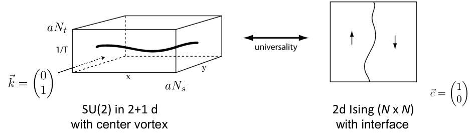
In two dimensions these universal numbers,
| (61) |
for all cyclic boundary conditions and all Potts models with order transitions, i.e., for , and , follow from the exact expressions of the corresponding partition functions at criticality obtained in Ref. [105]. In terms of Jacobi elliptic theta functions,
| (62) |
and with the definitions (for square lattices),
| (63) | ||||
the partition functions of the -state Potts models with different cyclic boundary conditions at criticality can be expressed [105], for the Ising model with as,
| (64) | ||||
for the state Potts model as,
| (65) | ||||
and the distinct ones for as
| (66) | ||||
Generally, the partition functions obey and . The ratios readily follow.
These universal ratios can be used to determine the critical couplings of the transition in the 2+1 dimensional gauge theories with high precision [106], by requiring that at with and the corresponding boundary conditions. For SU in dimensions, for example, where,
| (67) |
from the 2 square Ising model, this was used in [106] to determine the critical couplings of the deconfinement transition for lattices with up to links in the Euclidean time direction with a precision typically two orders of magnitude better than previous literature values where they were available [107, 108, 99]. In particular, the high precision allows to reliably determine the subleading -corrections to the linearly increasing behavior of with near the continuum limit in dimensions,
| (68) | ||||
The slope of the leading term determines the critical temperature in units of the dimensionful continuum coupling of the (2+1) theory, yielding . By standard arguments, from this result one can also read off the temperature dependence of the coupling at a given [106],
| (69) |
For each fixed , we thus have precise control of the temperature , where is the lattice spacing, by varying the lattice coupling . The physical length of the spatial volume then follows from
| (70) |
3.2 Twisted boundary conditions,
electric and
magnetic center flux
As mentioned above, the different choices of twisted b.c.’s in pure SU gauge theories at finite temperature are labeled by two -valued vectors, and , and fix the total numbers of vortices mod through the orthogonal planes of the Euclidean spacetime box as sketched in Fig. 16. There are purely spatial planes and the -dimensional vector denotes the total conserved, -valued and gauge-invariant magnetic flux through those, as generated by a static center monopole. The ones through the temporal planes labeled by the -dimensional vector are the universal partners of the Potts interfaces.
In order to understand the inequivalent choices for imposing boundary conditions on the gauge fields , which are blind to the center of SU, one first chooses to be periodic with the lengths of the system in each direction up to gauge transformation , which is physically equivalent to periodic boundary conditions,
| (71) |
In the box at finite temperature, we use
| (72) |
Then, compatibility of two successive translations in a ()-plane requires that (no summation of indices)
| (73) | ||||
The total number modulo of center vortices in a ()-plane is specified in each sector by the corresponding component of the twist tensor . In spatial dimensions magnetic center flux through the box is given by , in by . The time components define the temporal twist .

With these inequivalent choices of boundary conditions, the finite-volume theory in dimensions decomposes into sectors of fractional Chern-Simons number () [109] with states labelled by , where the integer is the usual instanton winding number. These sectors are connected by homotopically non-trivial gauge transformations ,
| (74) |
Note that such a gauge transformation must be multivalued in SU and hence singular to change the twist.
A Fourier transform of the twist sectors , which generalizes that for -vacua as Bloch waves from -vacua in two ways, by replacing for fractional winding numbers, and with an additional -Fourier transform w.r.t. the temporal twist , yields,
| (75) |
Up to a geometric phase,
| (76) |
the states in the new sectors are then invariant under the non-trivial also,
| (77) |
Their partition functions are classified, in addition to their magnetic flux and vacuum angle , by their -valued gauge-invariant electric flux in the -direction [90, 110]. Here, we do not consider finite and omit the argument in the partition functions henceforth. Magnetic flux is irrelevant for the deconfinement transition also, because for all combinations of magnetic flux with either electric flux or temporal twist [104],
| (78) |
There is no analogue of magnetic center flux in the spin systems, and center monopoles always condense because they are screened by the spatial string tension which is non-zero on either side of the deconfinement transition, likewise. Different combinations of temporal and spatial -twists, with different fractional topological charge, can however be used to measure the topological susceptibility without cooling [111].
The essential structure here is, however, that the temporally twisted vortex ensembles in the dimensional pure SU gauge theory are related to those with fixed units of electric flux (and a perhaps more intuitive physical interpretation) by a -dimensional discrete -Fourier transform [90],
| (79) |
no matter what the magnetic flux is, which is why the argument is dropped here and in the following also.
The role of the electric flux ensembles is best understood in terms of the translationally invariant flux between a fundamental color charge at some point in the finite volume and its mirror charge at in a neighboring volume in the direction of the flux [112],
| (80) |
where the ’s are untraced fundamental Polyakov loops, including any potentially non-trivial transition function in the time direction. With time-ordering from right to left,
| (81) |
The gauge field at differs from that at by the gauge transformation and we must undo this to make gauge invariant also under non-periodic gauge transformations which change the transition functions as
| (82) |
With this, the Polyakov line in Eq. (81) transforms as
| (83) |
and its trace is invariant under such gauge transformations even when .
In order to derive Eq. (80) we first decompose the total electric flux vector , with , and perform successive translations by in the direction of the individual unit vectors . For each step we use the boundary conditions (71) for the gauge fields and the cocycle condition (73) for the transition functions , to show that in a fixed twist sector with boundary conditions , and ,
| (84) |
where we have used to denote the normal Polyakov line as suitable for periodic boundary conditions. If we repeat this step for an arbitrary translation by , we pick up a product of center elements for the twists along the way,
| (85) |
and stands for the product of spatial transition functions when going from to . Changing the order of two spatial steps in different directions, in the path from to , multiplies by the corresponding spatial twist . Because , their order does therefore not matter in Eq. (85). We have,
| (86) |
in an ensemble with fixed temporal twist . When all boundary conditions are spatially periodic, . We can then insert the unity in Eq. (86) into the partition functions with fixed boundary conditions and sum over all temporally twisted sectors to establish Eq. (80) from Eq. (79). The subscript ‘no-flux’ in Eq. (80) indicates that the expectation value is meant to be taken in the enlarged ensemble corresponding to this sum. If there is no magnetic flux, , we can always apply time-independent (non-periodic) gauge transformations with
| (87) |
We can thus assume without loss that , as in Eq. (80) which then remains manifestly invariant under spatially periodic gauge transformations in this form. When we can still use Eq. (80) for a single direction, but for diagonal electric fluxes in a plane with magnetic twist we must include the combination of spatial transition functions in the expectation value on the right as in Eq. (86) which is then, however, invariant under non-periodic gauge transformations as well.66 6 This slight subtlety was overlooked in [112]. To verify the invariance of Eq. (86) under general, non-periodic gauge transformations is a straightforward exercise in manipulating transition functions using their cocycle condition (73) and transformation law (82).
Eq. (80) emphasizes the physical interpretation of the electric flux sectors, as providing the necessary mirror charges for the sectors of SU with non-vanishing total color charge, dual to those with fixed boundary conditions. Unlike the standard product of static charges at distance in a periodic ensemble, which is not gauge invariant, the electric fluxes (80) determine the gauge-invariant color-singlet free energy or potential between static charges at distance . They contain no ultraviolet divergent perimeter terms and no short-distance Coulomb contributions either.
3.3 Electric fluxes and selfduality in dimensions
Independent of universality and scaling, exact maps between the spin systems and their dual theories, in terms of disorder variables on the dual lattice, are provided by Kramers-Wannier duality [113]. In 2 dimensions, the dual of a spin model is a spin model again. In particular, the 2 -state Potts models (57) are selfdual for all . In dimensions, the spin models are dual to gauge theories. The best known example is the Ising model whose dual partner is the gauge theory, and this system is relevant for the dual universal behavior of center vortex and electric flux ensembles in the dimensional SU gauge theory [112, 114]. In 4 dimensions, the dual of a gauge model is a gauge model again [113].
One particular aspect of the SU gauge theories in dimensions with , and , that has been overlooked until recently, follows from the selfduality of the corresponding 2 -state Potts models and universality. The center vortex and electric flux ensembles of the dimensional gauge theories are mirror images of one another within the universal scaling window around criticality [115, 116, 100]. This is obvious from the fact that, as we will see, the exact duality transformation of the 2 -state Potts models in a finite volume is precisely of the structure of ’t Hooft’s relation between the temporal center vortex and electric flux ensembles in Eq. (79) discussed above.
The duality transformation and the selfduality of the -state Potts models in 2 dimensions has long been known for infinite systems. A particularly simple proof based on the random bond-cluster representation was given in [93]. Far less is known in a finite volume with translationally invariant boundary conditions, however, where ensembles with different boundary conditions in general mix under duality transformations. One case where this is known is the 3 Ising/-gauge theory system [117, 118, 119]. For the Potts model, using the random cluster methods developed in [105], we were able to obtain the following exact duality transformations for all on a finite 2 torus as discrete 2 Fourier transforms over all ensembles with cyclically shifted boundary conditions [115],
| (88) |
where is the total number of sites of the 2 lattice (i.e., on an square lattice), is the coupling per temperature, and its dual obtained from
| (89) |
as usual, with temperature mirrored around criticality at
| (90) |
For , and with , conventionally, this duality relation reduces to an analogous known result for the Ising model [120]. With it agrees with a result obtained for the planar or vector Potts model [121] which is equivalent to the standard one in that case.
Before we turn to the sketch of the proof, note that the structure of the finite-volume duality transformation in the Potts models (88) is precisely the same as that in the relation between the temporal center vortex and electric flux ensembles in Eq. (79). The temporal center vortices are the universal partners of the interfaces in the spin model, c.f., Fig. 15, and the electric fluxes are their duals, with again universally related to ensembles with interfaces, but at the dual temperature, swapped around criticality. In spatial dimensions the pattern is the same [114], the center vortex free energies in SU share their universal behavior with those of the interfaces in the Ising model, and electric fluxes correspond to ensembles of the dual gauge theory with anti-periodic boundary conditions. But they are not exact mirror images of one another in .
The general formula (88), for all -state Potts models on a 2 torus, was first given to my knowledge in [115].
I have not published its proof nor have I seen it in the literature before. So I will sketch it here, in the rest of this subsection which will not be needed later on and which the reader may thus choose to skip ad libitum.
The proof uses mostly standard techniques [122, 93], and it is based on the setup and results of Ref. [105].
We start from the Hamiltonian (57) without external field () but with cyclic interfaces such that
| (91) |
where the notation is such that we have introduced matrices on the links connecting nearest neighbors , and when and zero otherwise. For the cyclic interfaces we introduce straight lines (seams) and in the and directions on the dual lattice and use
| (92) |
where is a matrix for an elementary cyclic shift,
| (93) |
such that along the -direction the spins get shifted times at the links dual to (i.e., crossing) and times in the -direction at those dual to . The cyclically shifted boundary conditions implemented in this way are special cases of the general permutations of spin states across the boundary considered in Ref. [105]. We will use the random-cluster representation of the Potts models on a finite torus from there. With
| (94) |
the random-cluster representation of the partition function with -boundary conditions then follows from
| (95) | ||||
This is the standard random-cluster representation of the infinite Potts models [123, 122, 93]. It is valid also on the torus in this form as long as we only consider the cyclic shifts of the spin states across the seams in Eq. (92) as will be shown below. The product in the second line is multiplied out and the spin sum represented as a sum over all graphs where a link with aligned spins, , is said to be occupied while those with are empty. The possible configurations are then identified with graphs consisting of clusters connected by occupied links, whereby each disconnected site counts as its own cluster. So all sites are part of a cluster. Each occupied link (or bond) in a graph contributes a factor , and their total number in a given graph is called . Each of the clusters in a graph can be flipped independently as a whole and thus gives a combinatoric weight to the particular graph in the partition sum.
On the torus one needs to classify the clusters by the possible winding numbers of the non-selfintersecting closed loops around the torus that one can draw on them:
– If one cluster extends across both boundaries in such a way that independent and loops are possible, the graph is said to have a torus cluster (TC) of which it can have at most one.
– A cylinder cluster (CC) extends across the boundaries in such a way that only non-trivial loops with winding numbers are possible, where and are coprime. We call the number of cylinder clusters in a graph , and they must all have the same pair of winding numbers.
– And finally, island-type clusters are the ones on which only loops are possible. A graph with only island-type clusters is called a torus lake (TL) because the empty links form stacks which extend across the boundaries in both directions such that independent and loops are possible on the dual lattice, perpendicular to these stacks.
Generally, the empty links on the original lattice are dual to links which can be connected to form a cluster on the dual lattice . Therefore, a lake on the original lattice is a cluster on the dual lattice [105].
With this classification, and more general seams corresponding to arbitrary and independent permutations and of the spin states across each boundary in and directions the random cluster formulation of the Potts models on the torus as derived in [105] becomes,
| (96) |
Here this simplifies to,
| (97) |
The first sum is over all graphs with cylinder clusters, the second over all graphs with one torus cluster and the third over all graphs with only island-type clusters in a torus lake. See Ref. [105] for more details.
In the second line (97) we have used that and here, and that the weight of an cylinder cluster from [105] then reduces to
| (98) |
whereby, with the Kronecker delta modulo ,
| (99) | ||||
Moreover, unlike the more general case with arbitrary permutations , in [105], for the cyclic ones in Eq. (92) considered here, a torus cluster is only possible when , i.e., with periodic boundary conditions. But then it can have different states just as any other island-type cluster, therefore
| (102) |
This means that when we restrict to cyclically shifted boundary conditions, all clusters that are possible for such given boundary conditions have the same weight, , and this establishes that the infinite volume form of the cluster representation in Eq. (95) remains formally valid. One only needs to figure out the allowed cylinder and torus cluster and torus lake graphs as in Eq. (97) which is the starting point for the duality transformation in the finite volume.
The first task in obtaining the dual cluster representation is to re-express the number of occupied links and the number of clusters in Eq. (97) in terms of the corresponding numbers on the dual lattice .
To achieve this, recall that for an arbitrary lattice, the Euler formula relates the number of vertices , edges , faces , and open ends to the genus of the surface on which it is drawn via the Euler characteristic,
| (103) |
The Euler characteristic of the torus with and without open ends, , is . Moreover, is the number of sites of , and is the total number of links, that is the sum of occupied ones and empty ones which is identical to the number of occupied ones on the dual lattice . Thus . Finally, the number of faces is the number of sites on , i.e., . Therefore
| (104) |
It also follows from the Euler relation on the torus with that the total number of sites of the lattice is given by the number of clusters in a graph (recall that every site is part of a cluster) plus the number of occupied links minus the number of independent non-homotopic (and non-selfintersecting) loops on the clusters of the graph. Therefore, the number of clusters in a graph is expressed as
| (105) |
All TC graphs, with one torus cluster on the original lattice, are graphs with one torus lake on the dual lattice and vice versa, i.e., and .
On a TL graph, where all clusters are islands whose coastlines have winding numbers, one can walk around every pond which is a lake with coastline inside a cluster. Therefore . On a TC graph, one can walk around all ponds individually, but walking around all of them is homotopic to a point. In addition there are the and loops, thus . Together with the fact that the islands of a TL graph are the ponds of its dual graph TC∗ and vice versa, this implies for
| (106) | ||||
The ponds become islands on the dual graph. So is equal to the number of dual clusters on TL∗ graphs, while is the number of islands (and thus ) plus one on TC∗ graphs.
If we insert the identities (106) together with the Euler relation (104) into Eq. (105), this leads to
| (107) | ||||
| (108) |
CC graphs are selfdual. They contain an equal number of cylinder clusters and cylinder lakes, and all of them have the same winding numbers . The dual graph is the one with clusters and lakes swapped, and it thus has the same number of cylinder clusters, , with the same set of winding numbers. On a CC graph one can walk non-homotopically around every pond and along the loop of every cylinder cluster, therefore,
| (109) |
Now we use the relations in Eqs. (104), (107), (108), and (109), to re-express and in Eq. (97) in terms of the corresponding numbers and on the dual lattice . Labeling the graphs in the sums by their respective dual cluster configurations, this yields for the partition function with boundary conditions,
| (110) |
and its discrete Fourier transform over becomes,
| (111) | ||||
We have factorized another in Eq. (111) to get the right power in the middle term for which the sums over and collapse to the single term. The additional factor in front of the last term in Eq. (111) arises because the TL graphs are independent of the boundary conditions and and therefore their sums yield and , respectively. In the first term, the graph sum extends over all kinds of graphs with cylinder clusters for all pairs of coprime windings and , and the periodic Kronecker delta,
| (112) |
selects the right ones for each pair of boundary conditions . The duality transformation is thus completed upon realizing that for any pair of coprime , we can write,
| (113) | ||||
The last step might not be immediately obvious. It is verified by showing the following:77 7 I thank Nils Strodthoff for verifying that these two conditions are indeed satisfied.
(a) There is at most one in which solves the two conditions and at the same time. If it does, then the condition is also satisfied.
(b) If there is no solution to the first two conditions, then the new condition does not have one either.
Therefore, we have shown that the terms in brackets on the right in Eq. (111) agree with the random cluster representation (97) of a Potts model partition function with boundary conditions , and with the replacement which is equivalent to replacing the coupling per temperature by its dual according to their duality relation in Eq. (89). Analogously rewriting the prefactor on the right in Eq. (111) with Eq. (89),
| (114) |
and rearranging Eq. (111) to solve for the terms in brackets on the right, equalling , then finally yields the selfduality relation (88) of the -state Potts models (57) for all . The result here is actually a bit more general than that given in (88) where we have used for a square lattice. More generally, the duality relation valid for any lattice on a torus without open ends, and symmetric in and , here follows from Eq. (111) as
| (115) | ||||
At criticality, with , the prefactors cancel and one verifies that the values of the partition functions for the various cyclic boundary conditions in Eqs. (64), (65), and (66) reproduce themselves under the discrete Fourier transform (115) for , and as they must. The finite-volume duality relation is valid, however, for all , including with first order transition.
In the 2+1 dimensional gauge theories, temperature is the same on both sides of the -Fourier transform in Eq. (79). As a consequence of the selfduality of the corresponding spin models, however, the free energies of spatial center vortices and those of the confining electric fluxes are mirror images of one another within the universal scaling window around the second order phase transition.
3.4 Universality and finite-size scaling
The ratios of partition functions with -twisted and periodic boundary conditions in the SU gauge theories are obtained from multiplying coclosed stacks of plaquettes by the center elements such that one plaquette in every plane of orientation is multiplied by the corresponding to the twist tensor (c.f., Eqs. (73)),
These coclosed stacks of plaquettes are dual to non-homotopic closed surfaces or lines on the dual lattices in or dimensions, respectively.
If the total number of plaquettes in all stacks is , the ratio of partition functions in (3.4) can be converted into a product of ratios, each of which represents the expectation value of the twisted plaquette in an ensemble with already twisted ones, where runs lexicographically through the plaquettes of one stack after another, to implement twisted b.c.’s in all -planes according to the non-zero components of the twist tensor ,
| (118) |
In this way, one ratio of partition functions requires independent Monte-Carlo simulations [124, 112].
For the temporal -twists one introduces coclosed stacks aligned with the time direction between one pair of adjacent time-slices, where they are dual to spatial lines in and surfaces in dimensions, just as the respective spin interfaces in and dimensions as illustrated in Fig. 15 above.
Once the reduced temperature is determined in terms of the lattice coupling , as from Eq. (69) for dimensional SU, and with the spatial lattice size from Eq. (70), a finite-size-scaling analysis can be performed. In the vicinity of the order phase transition generalized couplings such as the vortex-ensemble ratios , for sufficiently large , only depend on the ratio of and the large correlation length which in the infinite volume diverges as
| (119) |
with the correlation-length critical exponent , where for the 2 Potts models for (percolation), for (Ising model), for and for [122] . Here we are particularly interested in the ratios which, up to finite size corrections on an square lattice, depend on in a universal way. The corresponding universal scaling functions for the interface free energies per temperature, suppressing the indices for the boundary conditions, are given by
| (120) | ||||
where , , and stands for the universal ratio with the particular combination of boundary conditions that is being used in the , and state Potts models as per Eqs. (64), (65) or (66).
For the square Ising model, with , the finite volume partition functions have been obtained exactly for all combinations of periodic and anti-periodic boundary conditions in Ref. [125]. We can use these results for the ratios and to obtain the corresponding universal scaling functions from Eq. (120). In Fig. 17, we plot for the interface, for example, over for and . We have tested that the difference between and vanishes as with [106]. The corresponding small residual finite-volume effects are observed, e.g., in the deviation of the result around from that for . To check which lattice size is needed for any desired accuracy, one can calculate the deviations of from the asymptotic slope for which is also known analytically.
Generally, the interface tensions (per temperature) in the dimensional spin models are defined in the ordered phase as
| (121) |
Comparison of this definition with Eqs. (120) thus entails that, if is finite in this limit, the interface tensions near criticality must behave as
| (122) |
The exponent of the interface tension is tied to the correlation length exponent by one of the so-called hyperscaling relations. In particular, for the square Ising model with one antiperiodic direction, with and thus , the asymptotic slope follows from Onsager’s famous result [126], valid for all in the ordered phase with , for the tension of a straight interface in the thermodynamic limit,
| (123) |
When the spin-coupling per temperature is expanded about criticality at this leads to,88 8 We use the typical Ising model conventions for such that here as compared to the general Potts model formulae above.
| (124) |
and this agrees with the asymptotic slope of for in Fig. 17 as obtained from the exact finite volume partition functions and of Ref. [125].
Many alternative and simplified derivations of Onsager’s result (123) were given since then and can be found in text books [122, 127]. A particularly interesting one for us is given in Baxter’s book [122], as it provides the tension of a diagonal interface. In our notations his result can be written as
| (125) |
As the free energies so far, these are all interface tensions per temperature. The proper free energy of an interface is given by . The corresponding proper interface tensions,
| (126) |
per coupling over temperature, for to , following from Eqs. (123) and (125) are compared in Fig. 18. At , every antiferromagnetic bond-coupling costs in energy. The diagonal or zigzag interface is twice as long as the straight one. It needs twice as many antiferromagnetic couplings, hence, in units of , for the straight and for the diagonal interface. In the isotropic limit, when the correlation length is much larger than the lattice spacing, on the other hand, the underlying lattice does not matter anymore and the diagonal interface through a large finite volume is only a factor of longer than the straight one, i.e., from Eq. (125) around ,
| (127) |
The same square-root ratios near are observed for the Ising interfaces [128],
| (128) |
The spin-interface tension corresponds to the dual string tension for spatial center vortices in and spatial ’t Hooft loops in dimensions for which a dual area law holds in the high-temperature -broken phase. The same square root ratios (128) are observed for the dual string tension in SU [112, 114]. From the duality Eq. (79), on can show that they then must also hold for the electric fluxes in the confined -disordered phase below , and they are interpreted as the smoking gun of string formation: The free energy of orthogonal fluxes is minimized when their length is, i.e., when diagonal strings through the volume form.
At least for the dimensional SU gauge theory string formation just below the deconfinement transition temperature is thus proven from universality and the observed square-root ratios of the exact Ising model interface tensions in the isotropic limit.
Unlike the spin models, however, whose interface tensions at follow ratios as for isotropic flux, the electric fluxes in the SU gauge theories are expected to also show the square-root ratios for string formation at zero temperature. The numerical evidence from early Monte-Carlo results on the lattice is affirmative that this is indeed the case [129].
The (2+1) SU vortex-ensemble ratios were calculated on lattices for to , each with spatial sizes up to and in a suitable window of lattice couplings around to test the finite-size scaling (FSS) in Refs. [106, 115, 116]. For each fixed one generally observes very good scaling of the available data for all when plotted over the FSS variable . With , the physical spatial length from Eq. (70) in units of , and the reduced temperature from the lattice coupling via Eq. (69), we define,
| (129) |
For the resulting vortex free energies , for and , we then obtain accurate one-parameter fits via
| (130) |
to the exact universal scaling functions for and b.c.’s computed from the results of Ref. [125] as in Fig. 17. This determines the single non-universal parameter which is dimensionless and relates the SU FSS variable to the Ising one,
| (131) |
whereby the minus sign reflects the interchange of high and low temperature phases between the two.
How hard it is to precisely determine the dual string tension directly from the data for the vortex free energy is shown in Fig. 19. We need to get to asymptotically large , c.f., Eqs. (120), but that requires larger and larger in order to stay within the universal scaling window for sufficiently small . Note that here roughly amounts to in Fig. 17 where is not large enough to suppress finite-size corrections even in the Ising model. The computational costs in the dimensional gauge theory roughly increase as so it becomes rather expensive to beat the FSS corrections to the dual string tension by brute force, and this was observed even more so in [112].
Here, our one-parameter fits to the vortex free energies as per to the exact universal scaling functions help tremendously because we can obtain accurate data at comparatively low computational costs for these fits from small values, i.e., small volumes. Once is fixed, however, we can compute the dual string tension and, as we will see, also the string tension for electric flux from these.
This is because with the hyperscaling relations , the product of interface tension and correlation length, is independent of near criticality. In fact, this product is another example of a universal amplitude ratio [8]. To be precise, if we use the so-called exponential correlation length in the disordered phase of the spin model above , , then the universal constant is given by
| (132) | ||||
The results are again exact [93, 122, 127],99 9 The result is found in any of the textbooks, for it follows from the hard hexagon model [122], and for probably from the Baxter-Wu (triangular three-spin) model [130, 122], but I am unsure about the status of a mathematical proof of the latter. while the Ising ratio is determined numerically, e.g., see the review in Ref. [8].
The exponential correlation length corresponding to on the gauge theory side is that of the Polyakov loops in the confined phase below , which is given by the string tension and temperature as
| (135) |
Therefore, we have a universal relation between the string tension per below , playing the role of in Eq. (132), and the dual string tension above , as the interface tension in Eq. (132),
| (136) | ||||
where we have introduced an unknown non-universal constant which drops out from the universal ratio, and we have replaced one factor by in the string tension in second line as we work at leading order in the reduced temperature here. Instead of determining the constant from the vortex free energies in the high temperature phase at asymptotically large , here we can use the exact universal scaling function from the Ising model: We know the asymptotic slope of which is , therefore, from
| (137) |
Once we extract from our one-parameter fits at small where we have very accurate data, this then equally accurately determines the string tension and its dual around . Moreover, we can determine this single non-universal parameter for which allows a polynomial fit,
| (138) |
with the extrapolated result [115]. This then determines the leading behavior of the continuum string tension and its dual around the phase transition,
| (139) |
Once we have fixed the single non-universal parameter we can plot the calculated center vortex free energies or the corresponding ratios in comparison with as in Fig. 20 for . The data for all different spatial lattice sizes collapse beautifully onto the universal curve, the finite-size scaling description works rather well. Together with the corresponding result for two orthogonal center vortices we can perform the -Fourier transform (79) to obtain the ratios of electric flux over the no-flux ensemble in Eq. (80),
| (140) |
These are equally well described by without refitting the non-universal parameter , they are mirror images of the in a surprisingly large scaling window around criticality as seen in the right panel of Eq. (80), where we swapped for the electric fluxes to demonstrate that. This is the manifestation of the selfduality of the corresponding spin model.
Moreover, if we rescale the FSS variables by the parameters determined from the one-parameter fits for the individual data sets, the scaling of the data over all spatial lattice sizes can be extended to include different lattices. With this renormalization, one thus essentially obtains good continuum results already with the coarsest lattice here, as seen in the zoom-in plot around criticality in Fig. 21. The rescaled -range there, roughly corresponds to in Fig. 20, and the dashed line is obtained from the universal scaling function as and thus now independent of . The slight deviations of the vortex free energy from this curve near seen here, are predominantly due to the leading finite-size corrections , analogous to what is being observed in the ordered phase of the Ising model in Fig. 17 at negative .
The selfduality of the underlying Potts model is also observed in the SU gauge theory [100], as shown in Fig. 22. The dashed line in this figure marks the universal ratio from Eqs. (65). The two independent ones that one can form on a symmetric lattice for evaluate to
| (141) | ||||
Even though the data in Fig. 22 was obtained on a quite small and lattice, the intersection point of the vortex and electric flux ensembles and is almost right on the universal line. To exploit selfduality, where possible, turns out to be the fastest converging method to determine critical couplings by far.
There is a long history of methods to extract critical couplings or temperatures from simulations in finite volumes, going back to using pairwise intersections of Binder cummulants on successively larger lattices [131]. Hasenbusch later demonstrated that the ratios of partition functions with different boundary conditions could be used in the same way to obtain a much more rapid convergence with very good estimates already from rather small lattices [132]. At criticality, these ratios tend to the universal values in the thermodynamic limit. In [106] it was therefore shown how to obtain critical couplings for gauge theories from intersecting the ratios of finite volume partition functions with these universal fixed points, once their values are known. For (2+1) SU(2) this led to an even much faster convergence than their pairwise intersections. At the time we thought this is the best method, but now look at the comparison of the results from [106] with the intersection points from selfduality in Fig. 23, again for SU in dimensions as a benchmark. Already with , and without any extrapolation, the result from selfduality is within the errors of the extrapolated best infinite volume result, from Ref. [106], as indicated by the narrow grey band in Fig. 23.
The reason for this impressive result is that the leading finite-size corrections do not change the position of the intersection point in . They only move it upwards along a straight vertical line with increasing in plots such as the one of Fig. 22.
To see this explicitly, first use a finite-size scaling ansatz for the vortex ensemble ratios as functions of the lattice coupling around criticality of the form
| (142) |
Defining pseudocritical couplings in a finite volume by requiring that for the method of [106] leads to,
| (143) |
These extrapolate to from large spatial lattice sizes at fixed numbers of time slices . As a byproduct this method gives numerical estimates of the correction to scaling exponent .
With selfduality, however, one must then have for like values of electric flux and and temporal twist at . In fact, it is straightforward to verify that then,
| (144) |
with the same coefficients and as in (142). Therefore, the leading finite-size corrections to when defined by cancel. At criticality,
| (145) |
so the leading corrections only move the intersection point of and vertically without shifting the so defined critical coupling.
The results for SU from the intersection points are compared to the extrapolated pseudocritical couplings from intersecting with its universal critical value via Eq. (143) in Tab. 1.
In 2+1 dimensions the critical couplings grow linearly with to leading order at large , c.f. Eq. (68), and the critical temperature in units of the dimensionful continuum coupling is given by the slope,
| (146) |
From the values for with , and in Tab. 1, one obtains for SU [100],
| (147) |
corresponding to with a zero temperature string tension from a weighted average of the four values in [133]. This is consistent with from [99].
Moreover, because the spatial center vortex free energies for sufficiently large depend only on , and at leading order in , when expanding
| (148) |
one expects the slope at to behave as
| (149) |
Our current best estimates from fitting these slopes are: for SU where one expects for the Ising model, for SU(3) where for the 2 3-state Potts model, and for SU as compared to for the Potts model. An update on our results including more on SU will be published elsewhere.
| () | () | Lit. | |
|---|---|---|---|
| 2 | 8.15309(11) | 8.15297(57) | 8.1489(31)† |
| 4 | 14.7262(9) | 14.7194(45) | 14.717(17)† |
| 6 | 21.357(25) | - | 21.34(4) ‡ |
| 8 | 27.84(12) | - | - |
For SU, the center symmetry alone does not uniquely specify the effective spin model to describe the dynamics of Polyakov loops. SU is a rank-three group and has three fundamental representations, , and . So even the simplest effective Polyakov-loop model will consist of two distinct real terms, with nearest neighbor couplings between loops in / representations and between loops in the representation, c.f. Ref. [134]. Depending on the relative weight between the two, the corresponding spin model could be any of the -symmetric Ashkin-Teller models with three energy levels per link and continuously varying critical exponents between the Potts model class with and , and that of the planar or vector Potts model, or simply the clock model, which corresponds to two non-interacting Ising models in this case with and . In between these limits the model corresponds to two interacting Ising models with spins and and it thus has two order parameters, the usual magnetic ones or , which are the same in the isotropic model, with critical exponent , and an electric one with exponent , with for the standard Potts model (), and for the non-interacting case () of the clock model [122].
The present conclusion from the studies in Refs. [97, 98, 99] is that the deconfinement transition in (2+1) SU(4) gauge theory is weakly order. We do observe, however, at least approximately at the length scales corresponding to our spatial lattice volumes, a universal scaling which seems closest to the standard Potts case [100]. The critical couplings from the universal amplitude ratios in Eqs. (66) are fully consistent with those determined independent of Potts scaling and universality, e.g., for we find from Eqs. (66) as compared to independent of that. The correlation length exponent is also consistent with and the data scales nicely for all volumes up to . This maybe still too small to see the order nature, and the conclusions may well depend on as well. But even if the transition is weakly order in the infinite volume () and continuum limits (), it seems legitimate to ask, why it is the standard Potts model universality that is observed before those limits are reached, and why not any of the other Ashkin-Teller models, and can we derive the correct effective Polyakov-loop model to demonstrate that?
3.5 Fractional electric charge and quark confinement
Center symmetry is explicitly broken and the finite temperature transition of QCD becomes a smooth crossover when dynamical quarks in the fundamental representation are included. This crossover at zero chemical potential is very well studied on the lattice [135, 136]. In presence of fields such as the quarks in QCD which faithfully represent the center of the gauge group, there are no twisted boundary conditions on the torus and therefore no center vortex ensembles to study. The detailed understanding of the deconfinement phase transition in the pure gauge theory might appear to be a rather academic exercise then.
This neglects the electric charge of quarks, however, which is commonly expected to only require small perturbative corrections. On the other hand, the inclusion of the quarks’ fractional electric charge is well known to lead to a global symmetry of the full fermion and Higgs sector of the Standard Model. This symmetry combines the centers of the color and electroweak gauge groups, see also [137], and [138] for a review. Since quarks carry fractional electric charges or , their color and electromagnetic phases in the pair of combined transformations,
cancel precisely. They act trivially on all other particles in the Standard Model, which are blind to the center of SU and carry integer electric charge. Electric charge is related to hypercharge and the third component of weak isospin by , with SU and quantized in units of . The symmetry is therefore generated by
| (150) |
which gives six elements including the identity.
A global symmetry brings with it the possibility of a phase transition characterized by spontaneous symmetry breaking. In this case, one expects the transition to be driven by topological defects (vortices) that carry both color and electromagnetic flux, that is, center vortices with an additional electromagnetic Dirac string [139, 140]. Could the physical realization of this symmetry have non-trivial implications for confinement and the phase structure of QCD as part of the Standard Model then? We have started to address this question recently in a toy model with half-integer electrically charged quarks in a two-color QCD world with electromagnetism [141, 142].
The starting point is QC2D plus electromagnetism with 2 flavors of Wilson fermions in dimensions. By including ‘up’ and ‘down’ quarks with fractional charges relative to the U gauge action, we obtain a model with a global symmetry. The lattice action is
| (151) |
where is the usual Wilson fermion action with the distinction that parallel transporters for quarks are products of SU color matrices and U phases,
| (152) |
The SU plaquettes and U plaquette angles are formed from and in the usual way. In this model, ’fractional charge’ means that the parallel transporters for quarks contain half the U angle relative to the ’s that appear in the plaquette angle . That is, an electromagnetic link for quarks appears as an link in the U gauge action. An important point is that the ’volume’ of the compact U is determined by the quarks, which carry the smallest quantum of electric charge. The range of is chosen such that we integrate over all possible electromagnetic transporters for the quarks, amounting to a double counting in the U gauge action and for all integer charged particles. This is consistent with the premise that our compact U is the result of symmetry breaking in a SU unified theory, e.g., see Ref. [143].
It is clear from Eq. (152) that a color center element SU combined with an electromagnetic phase act as the identity on the quarks. The model therefore retains a color and electromagnetic combined center symmetry, despite the introduction of dynamical quarks. This is the analog of the hidden symmetry of the Standard Model.

The results in [141, 142] indicate that the usual ordering of color links by the dynamical quarks is negated by the inclusion of fractional electric charge. This is understood by analogy with the spin systems. In QCD alone, terms in a loop expansion of the fermion determinant that wind around the temporal direction favor the center sector in which the traced Polyakov loop . They break center symmetry and lead to an ordering in much the same way as an external magnetic field does for the Potts model spins in Eq. (57). The inclusion of fractional electric charge in our model bestows quark loops with an additional U phase which may undo this effect. Consider, for example, the hopping expansion of the Wilson fermion action for time slices to leading order in the hopping parameter, ,
| (153) | ||||
If the U Polyakov loop angle for quarks is disordered, then the sector is no longer favored and the SU center symmetry is dynamically restored. The effect is analogous to placing a Potts model in a fluctuating magnetic field, or to the Peccei-Quinn mechanism [144], in which the coupling of the CP violating term in QCD to an axion field allows for the dynamical restoration of CP symmetry.
Since the parallel transporters for quarks possess a degree of freedom that the U gauge action is blind to, this is possible even in the Coulomb phase for integer electric charges. Indeed, the SU Polyakov loop in the toy model with half-integer charged dynamical Wilson quarks is indistinguishable from the quenched result at values of the hopping parameter, or the quark mass, that would otherwise cause a significant amount of ordering in standard 2-color QCD. As shown in Figure 24, this is equally true when the U links are totally disordered in the confined phase , and in the Coulomb phase at of the U. Since the U gauge action is blind to the disorder as seen by the quarks, i.e., , it is unable to remove it.
The quenched result in Fig. 24 reflects the second order nature of the phase transition of pure SU in the universality class of the Ising/ gauge system with typical finite-size corrections. It clearly turns into a crossover in full QC2D at as in the Ising model with a symmetry-breaking external field. When the half-integer electromagnetic charges are included, the SU Polyakov loop falls straight back onto the quenched curve indicating that there might be true disorder in the vacuum when QCD is embedded into the Standard Model.
This is not the full story, however. A comparison of the and meson masses in the toy model and in QC2D with equal hopping parameter and SU gauge coupling as in [145] reveals that the mass scales have changed dramatically in the toy model [142]. One plausible interpretation is that there is strong disorder even for which adds to the strength of the confining potential. This effect might be unphysical. One needs to go back and verify scaling of the masses (or correlation lengths) in physical units as the continuum limit is approached which might not even exist without unification in the toy model.
Meanwhile, we have explored the phase diagram at the leading order in the hopping expansion for , with the effective action in Eq. (153), which allows us to cheaply check our intuition about the resulting couplings of SU and U(1)em links, without having to worry about the chiral limit for . We thus take the leading-order hopping expansion at face value, as a model beyond its range of applicability as an approximation to the full toy model. This effective model then shares its qualitative features with a fractionally charged fundamental Higgs model [146].
Fig. 25 shows the results for the SU Polyakov loop in the effective SU model with the leading order interactions in Eq. (153), where the U phases are restricted to , which amounts to in the U gauge action. As increases, the disorder-order deconfinement transition of the SU Polyakov loop moves to smaller values of and sharpens dramatically. Note that in the combined limit , the plaquette-plaquette coupling in Eq. (153) forces the SU plaquettes to take the values . For very large the transition line should therefore terminate with the first order bulk transition of the gauge theory at [147]. As the SU plaquette is driven to unity for large , the U plaquettes corresponding to quark loops, , receive an effective coupling that suppresses disorder. The relevant U Polyakov loop remains disordered at small values of , but transitions to unity for large and (not shown). Due to the disorder transition, the model might have three distinct phases, the confined phase for small and small , the deconfined one for small but and a Higgs phase in the corner where both couplings and are large. We currently investigate the same effect of disorder from half-integer electric charge in the phase diagram of fundamental SU Higgs models [146].
Given the fractional electric charge of quarks and the existence of a global symmetry that relates the centers of the color and electroweak gauge groups, it may be misleading to study non-perturbative phenomena such as confinement and perhaps also dynamical mass generation in QCD alone. In the toy two-color model, the coupling of Wilson quarks with half-integer electric charge relative to a compact U has a dramatic effect on the color sector. This is not due to electromagnetic fluctuations which should have small effects deep in the Coulomb phase for large , but it can be due to a frozen disorder that the low energy theory inherits from the grand unified theory. Such frozen disorder could have an effect akin to a random external field in Potts models [148] which are known to have phase transitions where they would not otherwise have them, with constant external fields.
Here the SU Polyakov loop shows an order-disorder transition that is consistent with the spontaneous center symmetry breaking transition of the pure gauge theory at values of the hopping parameter where center symmetry is clearly explicitly broken in standard two-color QCD. This happens despite the fact that static quarks are now described by the combined SU and half-integer U loops which continue to show a crossover behavior. The scales of both transitions are still widely separated and this problem needs to be solved in such models.
Combined twisted boundary conditions are nevertheless possible with more than one gauge group and the corresponding center vortex ensembles might become relevant for a deconfinement phase transition in the standard model if its hidden center-like symmetry is relevant to the real world. Whether this is the case or not seems hard to decide without grand unification. Meanwhile one might want to find out whether SU models of the kind of our two-color toy model in the limit are at all suited as effective low energy theories for hadron physics. If we did have absolute confinement in the real world, separated by a true phase transition from the quark-gluon plasma, this would obviously make a conceptually and phenomenologically important difference as compared to our present understanding that quarks are only exponentially suppressed in a hadronic phase that is analytically connected to the high-temperature plasma.
4 Concluding remarks
Many interesting facets of strongly interacting matter can be studied in QCD-like theories. Changing the number of quark flavors, their masses or the number of colors often leads to simplifications or idealizations which allow to understand qualitative features and mechanisms from such powerful concepts as universality, scaling and finite-size scaling. They allow to relate phenomena from diverse areas of physics by often surprising analogies. The liquid-gas transition of nuclear matter, Heisenberg ferromagnets for chiral symmetry breaking, ultracold fermionic quantum gases with BEC-BCS crossover for two-color QCD at finite baryon density, the very well studied spin models and their dualities for the deconfinement transition and the electric fluxes in the pure gauge theories are some of the famous examples touched upon in these lecture notes.
The description of critical phenomena in statistical physics and quantum field theory is today synonymous with the renormalization group. Valuable introductory accounts of various aspects of the renormalization group have been given at this Schladming Winter School. I have presented some selected examples of applications of basic renormalization group concepts towards a better understanding of chiral dynamics at finite density, quark confinement, the different phases of strongly interacting matter at extremes of temperature or density, and the nature of the transitions between them.
Arguably, two of the most promising non-perturbative tools to study the QCD phase diagram at the moment are the functional renormalization group and lattice simulations, especially in combination. These two complement each other very well. Non-perturbative functional methods in general rely on additional assumptions. These can be guided by intuition, derive from fundamental requirements such as causality, locality or gauge invariance, or they can be backed up by results from other approaches as external input. This is what lattice simulations can provide where they are possible without fermion sign problem. Therefore, it will be extremely valuable to investigate and ultimately completely understand the phase diagrams of QCD-like theories such as two-color QCD or the gauge theory which don’t have this problem.
A lot of work in this direction has been done in two-color QCD as reviewed in Section 2. Here we are naturally interested in the functional renormalization group treatment which we have seen to be well capable of describing the effects of finite baryon density and the competing dynamics of collective mesonic and baryonic fluctuations. The bosonic nature of the baryons in two-color QCD with a BEC-BCS crossover provides interesting analogies, but I have argued that the impact of the finite baryon density on the chiral transition reveals a genuine effect. There are reasons to believe that there might not be enough chiral symmetry breaking left for a chiral phase transition and a critical endpoint at finite baryon density in the QCD phase diagram either. Suitable theories with fermionic baryons but without fermion sign problem seem to be the logical next step to study at finite density. The gauge theory is such a theory and the studies of its phase diagram have only just begun. The challenge there will be to disentangle finite density effects due to bosonic from those due to the fermionic baryons, an ideal task for the next combined effort with the functional renormalization group and lattice Monte-Carlo simulations.
The confinement problem is obviously a hard one. But a better understanding on a fundamental level even in the simple dimensional SU gauge theories from exact results seems worthwhile to work our way up from there. I found some of these results such as the selfduality reflected in the center vortex and electric flux ensembles quite enlightening and perhaps also unexpected. The models may not be realistic but the results are quite powerful, and who knows, perhaps we will eventually find that it wasn’t wasted but that combined vortices and disorder in the vacuum may be relevant when QCD is embedded in the Standard Model.
Acknowledgements
I much enjoyed this Schladming Winter School and I would like to thank the organizers Natalia and Reinhard Alkofer, Christian Fischer, Heimo Latal, Leopold Mathelitsch, and of course the Director of the School, Bernd-Jochen Schaefer.
There are many colleagues and friends to whom I’m indebted for collaborations and discussions. In relation to the material in these lecture notes I would like to mention especially Philippe de Forcrand, Jeff Greensite, Kurt Langfeld, Axel Maas, Jan Pawlowski, Jochen Wambach, Björn Wellegehausen, and Andreas Wipf.
Finally, but most importantly I thank my students. Most of the results from the last few years that I presented here, were obtained together with Sam Edwards and Nils Strodthoff, in particular. It has been my privilege and great pleasure to work with them.
Financial support from the Helmholtz International Center for FAIR within the LOEWE program of the State of Hesse, the Helmholtz Association Grant No. VH-NG-332, and the European Commission, FP7-PEOPLE-2009-RG, Grant No. 249203 is greatly acknowledged.
References
References
- [1] P. Braun-Munzinger, J. Wambach, Colloquium: Phase diagram of strongly interacting matter, Rev.Mod.Phys. 81 (2009) 1031–1050. doi:10.1103/RevModPhys.81.1031.
- [2] e. Friman, Bengt, e. Hohne, Claudia, e. Knoll, Jorn, e. Leupold, Stefan, e. Randrup, Jorgen, et al., The CBM physics book: Compressed baryonic matter in laboratory experiments, Lect.Notes Phys. 814 (2011) 1–980. doi:10.1007/978-3-642-13293-3.
- [3] P. Senger, V. Friese, [CBM], Nuclear matter physics at sis-100, https://www.gsi.de/documents/DOC-2011-Aug-29.html (02 2012).
- [4] L. McLerran, R. D. Pisarski, Phases of cold, dense quarks at large N(c), Nucl.Phys. A796 (2007) 83–100. arXiv:0706.2191, doi:10.1016/j.nuclphysa.2007.08.013.
- [5] P. Gerber, H. Leutwyler, Hadrons Below the Chiral Phase Transition, Nucl.Phys. B321 (1989) 387. doi:10.1016/0550-3213(89)90349-0.
- [6] J. Wambach, K. Heckmann, M. Buballa, Transport Properties of Strong-Interaction Matter, Acta Phys. Polon. to be published. arXiv:1111.5475.
- [7] K. Rajagopal, F. Wilczek, Static and dynamic critical phenomena at a second order QCD phase transition, Nucl.Phys. B399 (1993) 395–425. arXiv:hep-ph/9210253, doi:10.1016/0550-3213(93)90502-G.
- [8] A. Pelissetto, E. Vicari, Critical phenomena and renormalization group theory, Phys.Rept. 368 (2002) 549–727. arXiv:cond-mat/0012164, doi:10.1016/S0370-1573(02)00219-3.
- [9] J. Berges, D. Jungnickel, C. Wetterich, Two flavor chiral phase transition from nonperturbative flow equations, Phys.Rev. D59 (1999) 034010. arXiv:hep-ph/9705474, doi:10.1103/PhysRevD.59.034010.
- [10] B.-J. Schaefer, H.-J. Pirner, Renormalization group flow and equation of state of quarks and mesons, Nucl.Phys. A660 (1999) 439–474. arXiv:nucl-th/9903003, doi:10.1016/S0375-9474(99)00409-1.
- [11] J. Braun, B. Klein, P. Piasecki, On the scaling behavior of the chiral phase transition in QCD in finite and infinite volume, Eur. Phys. J. C71 (2011) 1576. arXiv:1008.2155, doi:10.1140/epjc/s10052-011-1576-7.
- [12] B. Klein, J. Braun, P. Piasecki, Scaling behavior in two-flavor QCD, finite quark masses and finite volume effects, PoS (Lattice 2011) (2011) 199. arXiv:1111.3247.
- [13] R. D. Pisarski, F. Wilczek, Remarks on the Chiral Phase Transition in Chromodynamics, Phys.Rev. D29 (1984) 338–341. doi:10.1103/PhysRevD.29.338.
- [14] S. Ejiri, F. Karsch, E. Laermann, C. Miao, S. Mukherjee, et al., On the magnetic equation of state in (2+1)-flavor QCD, Phys.Rev. D80 (2009) 094505. arXiv:0909.5122, doi:10.1103/PhysRevD.80.094505.
- [15] A. Bazavov, Chiral transition temperature and aspects of deconfinement in 2+1 flavor QCD with the HISQ/tree action, PoS (Lattice 2011) (2011) 182. arXiv:1201.5345.
- [16] C. Bonati, P. de Forcrand, M. D’Elia, O. Philipsen, F. Sanfilippo, Constraints on the two-flavor QCD phase diagram from imaginary chemical potential, PoS (Lattice 2011) (2011) 189. arXiv:1201.2769.
- [17] Y. Hidaka, L. D. McLerran, R. D. Pisarski, Baryons and the phase diagram for a large number of colors and flavors, Nucl.Phys. A808 (2008) 117–123. arXiv:0803.0279, doi:10.1016/j.nuclphysa.2008.05.009.
- [18] A. Andronic, D. Blaschke, P. Braun-Munzinger, J. Cleymans, K. Fukushima, et al., Hadron Production in Ultra-relativistic Nuclear Collisions: Quarkyonic Matter and a Triple Point in the Phase Diagram of QCD, Nucl.Phys. A837 (2010) 65–86. arXiv:0911.4806, doi:10.1016/j.nuclphysa.2010.02.005.
- [19] A. Maas, L. von Smekal, B. Wellegehausen, A. Wipf, The phase diagram of a gauge theory with fermionic baryons, preprint4 pages, 3 figures. arXiv:1203.5653.
- [20] J. Kogut, M. A. Stephanov, D. Toublan, On two color QCD with baryon chemical potential, Phys.Lett. B464 (1999) 183–191, 13 pages, 1 figure Report-no: ITP-SB-99-28, SUNY-NTG-99-23. arXiv:hep-ph/9906346, doi:10.1016/S0370-2693(99)00971-5.
- [21] J. Kogut, M. A. Stephanov, D. Toublan, J. Verbaarschot, A. Zhitnitsky, QCD - like theories at finite baryon density, Nucl.Phys. B582 (2000) 477–513, laTeX, 40 pages with 5 figures; corrected version published in Nucl. Phys. B Report-no: SUNY-NTG-00/11. arXiv:hep-ph/0001171, doi:10.1016/S0550-3213(00)00242-X.
- [22] K. Splittorff, D. Son, M. A. Stephanov, QCD - like theories at finite baryon and isospin density, Phys.Rev. D64 (2001) 016003. arXiv:hep-ph/0012274, doi:10.1103/PhysRevD.64.016003.
- [23] K. Splittorff, D. Toublan, J. Verbaarschot, Diquark condensate in QCD with two colors at next-to-leading order, Nucl.Phys. B620 (2002) 290–314. arXiv:hep-ph/0108040, doi:10.1016/S0550-3213(01)00536-3.
- [24] G. V. Dunne, S. M. Nishigaki, Two color QCD in 3-D at finite baryon density, Nucl.Phys. B654 (2003) 445–465. arXiv:hep-ph/0210219, doi:10.1016/S0550-3213(03)00034-8.
- [25] T. Brauner, On the chiral perturbation theory for two-flavor two-color QCD at finite chemical potential, Mod.Phys.Lett. A21 (2006) 559–570. arXiv:hep-ph/0601010, doi:10.1142/S0217732306019657.
- [26] T. Kanazawa, T. Wettig, N. Yamamoto, Chiral Lagrangian and spectral sum rules for dense two-color QCD, JHEP 0908 (2009) 003. arXiv:0906.3579, doi:10.1088/1126-6708/2009/08/003.
- [27] T. Kanazawa, T. Wettig, N. Yamamoto, Chiral random matrix theory for two-color QCD at high density, Phys.Rev. D81 (2010) 081701. arXiv:0912.4999, doi:10.1103/PhysRevD.81.081701.
- [28] T. Kanazawa, T. Wettig, N. Yamamoto, Singular values of the Dirac operator in dense QCD-like theories, JHEP 1112 (2011) 007. arXiv:1110.5858, doi:10.1007/JHEP12(2011)007.
- [29] A. Nakamura, QUARKS AND GLUONS AT FINITE TEMPERATURE AND DENSITY, Phys.Lett. B149 (1984) 391. doi:10.1016/0370-2693(84)90430-1.
- [30] S. Hands, J. B. Kogut, M.-P. Lombardo, S. E. Morrison, Symmetries and spectrum of SU(2) lattice gauge theory at finite chemical potential, Nucl.Phys. B558 (1999) 327–346. arXiv:hep-lat/9902034, doi:10.1016/S0550-3213(99)00364-8.
- [31] S. Hands, I. Montvay, S. Morrison, M. Oevers, L. Scorzato, et al., Numerical study of dense adjoint matter in two color QCD, Eur.Phys.J. C17 (2000) 285–302. arXiv:hep-lat/0006018, doi:10.1007/s100520000477.
- [32] S. Muroya, A. Nakamura, C. Nonaka, Study of the finite density state based on SU(2) lattice QCD, Nucl.Phys.Proc.Suppl. 119 (2003) 544–546. arXiv:hep-lat/0208006, doi:10.1016/S0920-5632(03)80452-8.
- [33] S. Chandrasekharan, F.-J. Jiang, Phase-diagram of two-color lattice QCD in the chiral limit, Phys.Rev. D74 (2006) 014506. arXiv:hep-lat/0602031, doi:10.1103/PhysRevD.74.014506.
- [34] S. Hands, S. Kim, J.-I. Skullerud, Deconfinement in dense 2-color QCD, Eur.Phys.J. C48 (2006) 193. arXiv:hep-lat/0604004, doi:10.1140/epjc/s2006-02621-8.
- [35] S. Hands, S. Kim, J.-I. Skullerud, A Quarkyonic Phase in Dense Two Color Matter?, Phys.Rev. D81 (2010) 091502. arXiv:1001.1682, doi:10.1103/PhysRevD.81.091502.
- [36] S. Hands, P. Kenny, S. Kim, J.-I. Skullerud, Lattice Study of Dense Matter with Two Colors and Four Flavors, Eur.Phys.J. A47 (2011) 60. arXiv:1101.4961, doi:10.1140/epja/i2011-11060-1.
- [37] L. Kondratyuk, M. Giannini, M. Krivoruchenko, The SU(2) color superconductivity, Phys.Lett. B269 (1991) 139–143. doi:10.1016/0370-2693(91)91465-8.
- [38] L. Kondratyuk, M. Krivoruchenko, Superconducting quark matter in SU(2) color group, Z.Phys. A344 (1992) 99–115. doi:10.1007/BF01291027.
- [39] R. Rapp, T. Schafer, E. V. Shuryak, M. Velkovsky, Diquark Bose condensates in high density matter and instantons, Phys.Rev.Lett. 81 (1998) 53–56. arXiv:hep-ph/9711396, doi:10.1103/PhysRevLett.81.53.
- [40] C. Ratti, W. Weise, Thermodynamics of two-colour QCD and the Nambu Jona-Lasinio model, Phys.Rev. D70 (2004) 054013. arXiv:hep-ph/0406159, doi:10.1103/PhysRevD.70.054013.
- [41] G.-f. Sun, L. He, P. Zhuang, BEC-BCS crossover in the Nambu-Jona-Lasinio model of QCD, Phys.Rev. D75 (2007) 096004. arXiv:hep-ph/0703159, doi:10.1103/PhysRevD.75.096004.
- [42] T. Brauner, K. Fukushima, Y. Hidaka, Two-color quark matter: U(1)(A) restoration, superfluidity, and quarkyonic phase, Phys.Rev. D80 (2009) 074035. arXiv:0907.4905, doi:10.1103/PhysRevD.80.074035,10.1103/PhysRevD.81.119904,10.1103/PhysRevD.80.074035,10.1103/PhysRevD.81.119904.
- [43] J. O. Andersen, T. Brauner, Phase diagram of two-color quark matter at nonzero baryon and isospin density, Phys.Rev. D81 (2010) 096004. arXiv:1001.5168, doi:10.1103/PhysRevD.81.096004.
- [44] M. Harada, C. Nonaka, T. Yamaoka, Masses of vector bosons in two-color dense QCD based on the hidden local symmetry, Phys.Rev. D81 (2010) 096003. arXiv:1002.4705, doi:10.1103/PhysRevD.81.096003.
- [45] T. Zhang, T. Brauner, D. H. Rischke, QCD-like theories at nonzero temperature and density, JHEP 1006 (2010) 064. arXiv:1005.2928, doi:10.1007/JHEP06(2010)064.
- [46] L. He, Nambu-Jona-Lasinio model description of weakly interacting Bose condensate and BEC-BCS crossover in dense QCD-like theories, Phys.Rev. D82 (2010) 096003. arXiv:1007.1920, doi:10.1103/PhysRevD.82.096003.
- [47] N. Strodthoff, B.-J. Schaefer, L. von Smekal, Quark-meson-diquark model for two-color QCD, Phys.Rev. D85 (2012) 074007. arXiv:1112.5401, doi:10.1103/PhysRevD.85.074007.
- [48] V. Gusynin, S. Sharapov, J. Carbotte, AC conductivity of graphene: from tight-binding model to 2+1-dimensional quantum electrodynamics, Int.J.Mod.Phys. B21 (2007) 4611–4658. arXiv:0706.3016, doi:10.1142/S0217979207038022.
- [49] Ultracold atoms and the Functional Renormalization Group, these Lecture Notes. arXiv:1204.4394.
- [50] S. Diehl, S. Floerchinger, H. Gies, J. Pawlowski, C. Wetterich, Functional renormalization group approach to the BCS-BEC crossover, Annalen Phys. 522 (2010) 615–656. arXiv:0907.2193, doi:10.1002/andp.201010458.
- [51] M. M. Scherer, S. Floerchinger, H. Gies, Functional renormalization for the BCS-BEC crossover, preprint (2010). arXiv:1010.2890.
- [52] T. D. Cohen, Functional integrals for QCD at nonzero chemical potential and zero density, Phys.Rev.Lett. 91 (2003) 222001. arXiv:hep-ph/0307089, doi:10.1103/PhysRevLett.91.222001.
- [53] P. Braun-Munzinger, J. Stachel, The quest for the quark-gluon plasma, Nature 448 (2007) 302–309. doi:10.1038/nature06080.
- [54] A. Andronic, P. Braun-Munzinger, J. Stachel, Thermal hadron production in relativistic nuclear collisions: The Hadron mass spectrum, the horn, and the QCD phase transition, Phys.Lett. B673 (2009) 142–145. arXiv:0812.1186, doi:10.1016/j.physletb.2009.02.014,10.1016/j.physletb.2009.06.021.
- [55] L.-y. He, M. Jin, P.-f. Zhuang, Pion superfluidity and meson properties at finite isospin density, Phys.Rev. D71 (2005) 116001. arXiv:hep-ph/0503272, doi:10.1103/PhysRevD.71.116001.
- [56] J. Xiong, M. Jin, J. Li, Pion superfluidity and meson mass in the PNJL model with a finite iso spin chemical potential, J.Phys.G G36 (2009) 125005. doi:10.1088/0954-3899/36/12/125005.
- [57] K. Kamikado, N. Strodthoff, L. von Smekal, J. Wambach, Quark-meson model study of QCD with isospin chemical potential, in preparation (2012).
- [58] M. G. Alford, A. Schmitt, K. Rajagopal, T. Schafer, Color superconductivity in dense quark matter, Rev.Mod.Phys. 80 (2008) 1455–1515. arXiv:0709.4635, doi:10.1103/RevModPhys.80.1455.
- [59] A. W. Steiner, S. Reddy, M. Prakash, Color neutral superconducting quark matter, Phys.Rev. D66 (2002) 094007. arXiv:hep-ph/0205201, doi:10.1103/PhysRevD.66.094007.
- [60] M. Huang, I. Shovkovy, Gapless color superconductivity at zero and at finite temperature, Nucl.Phys. A729 (2003) 835–863. arXiv:hep-ph/0307273, doi:10.1016/j.nuclphysa.2003.10.005.
- [61] M. Mitter, B.-J. Schaefer, N. Strodthoff, L. von Smekal, U-breaking ’t Hooft Determinant in a Quark-Meson Model with Fluctuations, in preparation (2012).
- [62] B.-J. Schaefer, J. M. Pawlowski, J. Wambach, The Phase Structure of the Polyakov–Quark-Meson Model, Phys.Rev. D76 (2007) 074023. arXiv:0704.3234, doi:10.1103/PhysRevD.76.074023.
- [63] B.-J. Schaefer, M. Wagner, J. Wambach, Thermodynamics of (2+1)-flavor QCD: Confronting Models with Lattice Studies, Phys.Rev. D81 (2010) 074013. arXiv:0910.5628, doi:10.1103/PhysRevD.81.074013.
- [64] T. K. Herbst, J. M. Pawlowski, B.-J. Schaefer, The phase structure of the Polyakov–quark-meson model beyond mean field, Phys.Lett. B696 (2011) 58–67. arXiv:1008.0081, doi:10.1016/j.physletb.2010.12.003.
- [65] J. Braun, H. Gies, J. M. Pawlowski, Quark Confinement from Color Confinement, Phys.Lett. B684 (2010) 262–267. arXiv:0708.2413, doi:10.1016/j.physletb.2010.01.009.
- [66] F. Marhauser, J. M. Pawlowski, Confinement in Polyakov Gauge, preprint (2008). arXiv:0812.1144.
- [67] On gauge invariant Wilsonian flows, Workshop on the Exact Renormalization Group, faro, Portugal. arXiv:hep-th/9901063.
- [68] J. Berges, N. Tetradis, C. Wetterich, Nonperturbative renormalization flow in quantum field theory and statistical physics, Phys.Rept. 363 (2002) 223–386. arXiv:hep-ph/0005122, doi:10.1016/S0370-1573(01)00098-9.
- [69] J. Polonyi, Lectures on the functional renormalization group method, Central Eur.J.Phys. 1 (2003) 1–71. arXiv:hep-th/0110026, doi:10.2478/BF02475552.
- [70] J. M. Pawlowski, Aspects of the functional renormalisation group, Annals Phys. 322 (2007) 2831–2915. arXiv:hep-th/0512261, doi:10.1016/j.aop.2007.01.007.
- [71] Introduction to the functional RG and applications to gauge theories, ECT* School on Renormalization Group and Effective Field Theory Approaches to Many-Body Systems, Trento, Italy. arXiv:hep-ph/0611146.
- [72] B.-J. Schaefer, J. Wambach, Renormalization group approach towards the QCD phase diagram, Phys.Part.Nucl. 39 (2008) 1025–1032. arXiv:hep-ph/0611191, doi:10.1134/S1063779608070083.
- [73] J. Braun, Fermion Interactions and Universal Behavior in Strongly Interacting Theories, J.Phys.G G39 (2012) 033001, 131 pages, 26 figures, 2 tables, review article. arXiv:1108.4449, doi:10.1088/0954-3899/39/3/033001.
- [74] C. Wetterich, Exact evolution equation for the effective potential, Phys.Lett. B301 (1993) 90–94. doi:10.1016/0370-2693(93)90726-X.
- [75] D. F. Litim, Optimized renormalization group flows, Phys.Rev. D64 (2001) 105007. arXiv:hep-th/0103195, doi:10.1103/PhysRevD.64.105007.
- [76] A. K. Das, Finite temperature field theory, World Scientific, Singapore, 1997.
- [77] M. Le Bellac, Thermal field theory, Cambridge Monographs on Mathematical Physics, Cambridge University Press, 1996, first paperback edition (with corrrections) 2000.
- [78] A. Roberge, N. Weiss, GAUGE THEORIES WITH IMAGINARY CHEMICAL POTENTIAL AND THE PHASES OF QCD, Nucl. Phys. B275 (1986) 734. doi:10.1016/0550-3213(86)90582-1.
- [79] V. Skokov, B. Stokic, B. Friman, K. Redlich, Meson fluctuations and thermodynamics of the Polyakov loop extended quark-meson model, Phys.Rev. C82 (2010) 015206. arXiv:1004.2665, doi:10.1103/PhysRevC.82.015206.
- [80] V. Skokov, B. Friman, K. Redlich, Quark number fluctuations in the Polyakov loop-extended quark-meson model at finite baryon density, Phys.Rev. C83 (2011) 054904. arXiv:1008.4570, doi:10.1103/PhysRevC.83.054904.
- [81] J. Braun, K. Schwenzer, H.-J. Pirner, Linking the quark meson model with QCD at high temperature, Phys.Rev. D70 (2004) 085016. arXiv:hep-ph/0312277, doi:10.1103/PhysRevD.70.085016.
- [82] B.-J. Schaefer, J. Wambach, The Phase diagram of the quark meson model, Nucl.Phys. A757 (2005) 479–492. arXiv:nucl-th/0403039, doi:10.1016/j.nuclphysa.2005.04.012.
- [83] O. Bohr, B. Schaefer, J. Wambach, Renormalization group flow equations and the phase transition in O(N) models, Int.J.Mod.Phys. A16 (2001) 3823–3852. arXiv:hep-ph/0007098, doi:10.1142/S0217751X0100502X.
- [84] B. Stokic, B. Friman, K. Redlich, The Functional Renormalization Group and O(4) scaling, Eur.Phys.J. C67 (2010) 425–438. arXiv:0904.0466, doi:10.1140/epjc/s10052-010-1310-x.
- [85] S. Holtmann, T. Schulze, Critical behavior and scaling functions of the three-dimensional O(6) model, Phys.Rev. E68 (2003) 036111. arXiv:hep-lat/0305019, doi:10.1103/PhysRevE.68.036111.
- [86] D. F. Litim, Critical exponents from optimized renormalization group flows, Nucl.Phys. B631 (2002) 128–158. arXiv:hep-th/0203006.
- [87] B. D. Serot, J. D. Walecka, Recent progress in quantum hadrodynamics, Int.J.Mod.Phys. E6 (1997) 515–631. arXiv:nucl-th/9701058, doi:10.1142/S0218301397000299.
- [88] W. Caudy, J. Greensite, On the ambiguity of spontaneously broken gauge symmetry, Phys.Rev. D78 (2008) 025018. arXiv:0712.0999, doi:10.1103/PhysRevD.78.025018.
- [89] L. Polley, U. Wiese, Monopole condensate and monopole mass in U(1) lattice gauge theory, Nucl.Phys. B356 (1991) 629–654. doi:10.1016/0550-3213(91)90380-G.
- [90] G. ’t Hooft, A Property of Electric and Magnetic Flux in Nonabelian Gauge Theories, Nucl.Phys. B153 (1979) 141.
- [91] S. Edwards, D. B. Mehta, A. Rajantie, L. von Smekal, ’t Hooft-Polyakov monopoles in lattice SU(N)+adjoint Higgs theory, Phys.Rev. D80 (2009) 065030. arXiv:0906.5531, doi:10.1103/PhysRevD.80.065030.
- [92] J. Greensite, The Confinement problem in lattice gauge theory, Prog.Part.Nucl.Phys. 51 (2003) 1. arXiv:hep-lat/0301023, doi:10.1016/S0146-6410(03)90012-3.
- [93] F. Wu, The Potts model, Rev.Mod.Phys. 54 (1982) 235–268. doi:10.1103/RevModPhys.54.235.
- [94] P. De Forcrand, L. Von Smekal, ’t Hooft loops and consistent order parameters for confinement, Nucl.Phys.Proc.Suppl. 106 (2002) 619–621. arXiv:hep-lat/0110135, doi:10.1016/S0920-5632(01)01796-0.
- [95] B. Svetitsky, L. G. Yaffe, Critical Behavior at Finite Temperature Confinement Transitions, Nucl.Phys. B210 (1982) 423. doi:10.1016/0550-3213(82)90172-9.
- [96] R. Baxter, Potts model at critical temperature, J.Phys.C C6 (1973) L445–L448.
- [97] P. de Forcrand, O. Jahn, Deconfinement transition in (2+1)-dimensional SU(4) lattice gauge theory, Nucl.Phys.Proc.Suppl. 129 (2004) 709–711. arXiv:hep-lat/0309153, doi:10.1016/S0920-5632(03)02688-4.
- [98] K. Holland, M. Pepe, U.-J. Wiese, Revisiting the deconfinement phase transition in SU(4) Yang-Mills theory in 2+1 dimensions, JHEP 0802 (2008) 041. arXiv:0712.1216, doi:10.1088/1126-6708/2008/02/041.
- [99] J. Liddle, M. Teper, The Deconfining phase transition in D=2+1 SU(N) gauge theories, preprint (2008). arXiv:0803.2128.
- [100] N. Strodthoff, S. R. Edwards, L. von Smekal, SU(3) Deconfinement in (2+1)d from Twisted Boundary Conditions and Self-Duality, PoS LATTICE2010 (2010) 288, 7 pages, 4 figures (pdflatex), for the proceedings of the XXVIII International Symposium on Lattice Field Theory, Lattice2010, June 14-19, 2010, Villasimius, Sardinia, Italy. arXiv:1012.0723.
- [101] T. Heinzl, T. Kaestner, A. Wipf, Effective actions for the SU(2) confinement-deconfinement phase transition, Phys.Rev. D72 (2005) 065005, 14 pages, 10 figures, v2: typos corrected Report-no: preprint FSU-TPI/03/05. arXiv:hep-lat/0502013, doi:10.1103/PhysRevD.72.065005.
- [102] C. Wozar, T. Kaestner, A. Wipf, T. Heinzl, Inverse Monte-Carlo determination of effective lattice models for SU(3) Yang-Mills theory at finite temperature, Phys.Rev. D76 (2007) 085004. arXiv:0704.2570, doi:10.1103/PhysRevD.76.085004.
- [103] J. Langelage, S. Lottini, O. Philipsen, Centre symmetric 3d effective actions for thermal SU(N) Yang-Mills from strong coupling series, JHEP 1102 (2011) 057. arXiv:1010.0951, doi:10.1007/JHEP02(2011)057,10.1007/JHEP07(2011)014,10.1007/JHEP02(2011)057,10.1007/JHEP07(2011)014.
- [104] L. von Smekal, P. de Forcrand, Electric and magnetic fluxes in SU(2) Yang-Mills theory, Nucl.Phys.Proc.Suppl. 119 (2003) 655–657, 3 pages, LaTeX2e (espcrc2.sty), 4 figures (epsfig), for Lattice2002(topology) Report-no: FAU-TP3-02/25. arXiv:hep-lat/0209149, doi:10.1016/S0920-5632(03)01633-5.
- [105] H. Park, M. den Nijs, Universal finite-size-scaling amplitudes of the Potts model on a torus, Phys.Rev. B38 (1988) 565–579. doi:10.1103/PhysRevB.38.565.
- [106] S. Edwards, L. von Smekal, SU(2) lattice gauge theory in 2+1 dimensions: Critical couplings from twisted boundary conditions and universality, Phys.Lett. B681 (2009) 484–490. arXiv:0908.4030, doi:10.1016/j.physletb.2009.10.063.
- [107] M. Teper, The Finite temperature phase transition of SU(2) gauge fields in (2+1)-dimensions, Phys.Lett. B313 (1993) 417–424. doi:10.1016/0370-2693(93)90012-7.
- [108] J. Engels, F. Karsch, E. Laermann, C. Legeland, M. Lutgemeier, et al., A Study of finite temperature gauge theory in (2+1)-dimensions, Nucl.Phys.Proc.Suppl. 53 (1997) 420–422. arXiv:hep-lat/9608099.
- [109] P. van Baal, Some Results for SU(N) Gauge Fields on the Hypertorus, Commun.Math.Phys. 85 (1982) 529. doi:10.1007/BF01403503.
- [110] G. ’t Hooft, Duality and Oblique Confinement, in: P. van Baal (Ed.), Confinement, duality, and nonperturbative aspects of QCD, NATO Advanced Study Institute, Plenum Press, New York, 1998, pp. 379–386.
- [111] More on electric and magnetic fluxes in SU(2), Quark Confinement and the Hadron Spectrum V, World Scientific, 2002. arXiv:hep-lat/0212019.
- [112] P. de Forcrand, L. von Smekal, ’t Hooft loops, electric flux sectors and confinement in SU(2) Yang-Mills theory, Phys.Rev. D66 (2002) 011504. arXiv:hep-lat/0107018, doi:10.1103/PhysRevD.66.011504.
- [113] R. Savit, Duality in Field Theory and Statistical Systems, Rev.Mod.Phys. 52 (1980) 453. doi:10.1103/RevModPhys.52.453.
- [114] L. von Smekal, P. de Forcrand, Electric flux sectors and confinement, in: J. Greensite, S. Olejnik (Eds.), Confinement, Topology and Other Non-Perturbative Aspects of QCD, NATO Science Series, Kluwer, Dordrecht, The Netherlands, 2002, pp. 287–294. arXiv:hep-ph/0205002.
- [115] L. von Smekal, S. R. Edwards, N. Strodthoff, Universal Aspects of Deconfinement: Interfaces, Flux Tubes and Self-Duality in 2+1 Dimensions, PoS LATTICE2010 (2010) 292. arXiv:1012.0408.
- [116] L. von Smekal, S. R. Edwards, N. Strodthoff, Universal Aspects of Deconfinement in 2+1 Dimensions, AIP Conf.Proc. 1343 (2011) 212–214. arXiv:1012.1712, doi:10.1063/1.3574980.
- [117] C. Gruber, A. Hintermann, D. Merlini, Group Analysis of Classical Lattice Systems, Springer, Berlin - Heidelberg, 1977.
- [118] M. Caselle, M. Hasenbusch, P. Provero, K. Zarembo, Bound states and glueballs in three-dimensional Ising systems, Nucl.Phys. B623 (2002) 474–492. arXiv:hep-th/0103130, doi:10.1016/S0550-3213(01)00644-7.
- [119] M. Hasenbusch, M. Caselle, private communications (2010).
- [120] Münster, Gernot, private communications (2001).
- [121] A. I. Bugrii, V. N. Shadura, Duality in 2-D spin models on torus, preprint, ITEP-TH-20-97 (1997). arXiv:hep-th/9706045.
- [122] R. J. Baxter, Exactly Solved Models in Statistical Mechanics, Dover, Mineola, N.Y., 2007, originally published by Academic Press, London, 1982, with new chapter.
- [123] C. Fortuin, P. Kasteleyn, On the Random cluster model. 1. Introduction and relation to other models, Physica 57 (1972) 536–564. doi:10.1016/0031-8914(72)90045-6.
- [124] P. de Forcrand, M. D’Elia, M. Pepe, A Study of the ’t Hooft loop in SU(2) Yang-Mills theory, Phys.Rev.Lett. 86 (2001) 1438. arXiv:hep-lat/0007034, doi:10.1103/PhysRevLett.86.1438.
- [125] M.-C. Wu, M.-C. Huang, Y.-P. Luo, T.-M. Liaw, Coupling-anisotropy and finite-size effects in interfacial tension of the two-dimensional Ising model, J. Phys. A: Math. Gen. 32 (1999) 4897–4906. doi:10.1088/0305-4470/32/26/308.
- [126] L. Onsager, Crystal statistics. 1. A Two-dimensional model with an order disorder transition, Phys.Rev. 65 (1944) 117–149. doi:10.1103/PhysRev.65.117.
- [127] C. Itzykson, J.-M. Drouffe, Statistical field theory, Monographs on Mathematical Physics, Cambridge, New York, 1989.
- [128] M. Pepe, P. De Forcrand, Finite size scaling of interface free energies in the 3-d Ising model, Nucl.Phys.Proc.Suppl. 106 (2002) 914–916. arXiv:hep-lat/0110119, doi:10.1016/S0920-5632(01)01884-9.
- [129] A. Hasenfratz, P. Hasenfratz, F. Niedermayer, ELECTRIC FLUXES AND TWISTED FREE ENERGIES IN SU(3), Nucl.Phys. B329 (1990) 739. doi:10.1016/0550-3213(90)90080-W.
- [130] R. Baxter, F. Wu, Exact Solution of an Ising Model with Three-Spin Interactions on a Triangular Lattice, Phys.Rev.Lett. 31 (1973) 1294–1297. doi:10.1103/PhysRevLett.31.1294.
- [131] K. Binder, Finite size scaling analysis of Ising model block distribution functions, Z.Phys. B43 (1981) 119–140. doi:10.1007/BF01293604.
- [132] M. Hasenbusch, Monte Carlo simulation with fluctuating boundary conditions, Physica A 197 (1993) 423–435.
- [133] B. Bringoltz, M. Teper, A Precise calculation of the fundamental string tension in SU(N) gauge theories in 2+1 dimensions, Phys.Lett. B645 (2007) 383–388. arXiv:hep-th/0611286, doi:10.1016/j.physletb.2006.12.056.
- [134] C. Wozar, T. Kaestner, A. Wipf, T. Heinzl, B. Pozsgay, Phase structure of Z(3)-Polyakov-loop models, Phys.Rev. D74 (2006) 114501. arXiv:hep-lat/0605012, doi:10.1103/PhysRevD.74.114501.
- [135] S. Borsanyi, et al., Is there still any mystery in lattice QCD? Results with physical masses in the continuum limit III, JHEP 1009 (2010) 073. arXiv:1005.3508, doi:10.1007/JHEP09(2010)073.
- [136] A. Bazavov, P. Petreczky, Deconfinement and chiral transition with the highly improved staggered quark (HISQ) action, J.Phys.Conf.Ser. 230 (2010) 012014, 16 pages, 17 figures, talk presented at the 26th Winter Workshop on Nuclear Dynamics, Ocho Rios, Jamaica, January 2-9, 2010, to be published in Journal of Physics: Conference Series (JPCS). arXiv:1005.1131, doi:10.1088/1742-6596/230/1/012014.
- [137] B. Bakker, A. Veselov, M. Zubkov, Standard model with the additional Z(6) symmetry on the lattice, Phys.Lett. B620 (2005) 156–163. arXiv:hep-lat/0502006, doi:10.1016/j.physletb.2005.06.029.
- [138] J. C. Baez, J. Huerta, The Algebra of Grand Unified Theories, Bull.Am.Math.Soc. 47 (2010) 483–552, 73 pages, 20 ps figures. arXiv:0904.1556.
- [139] M. Creutz, Are magnetic monopoles hadrons?, Nucl.Phys.Proc.Suppl. 140 (2005) 597–599. arXiv:hep-lat/0408013, doi:10.1016/j.nuclphysbps.2004.11.198.
- [140] L. von Smekal, T. Tok, P. de Forcrand, A Toy model of (grand) unified monopoles, PoS LAT2005 (2006) 314, poS(LAT2005)314, 6 pages, 3 figures, for the proceedings of ’Lattice 2005 (Topology and Confinement).’. arXiv:hep-lat/0509147.
- [141] S. R. Edwards, A. Sternbeck, L. von Smekal, Exploring a hidden symmetry with electrically charged quarks, PoS LATTICE2010 (2010) 275, 7 pages, 2 figures. Conference proceedings for the XXVIII International Symposium on Lattice Field Theory, 2010. arXiv:1012.0768.
- [142] S. R. Edwards, A. Sternbeck, L. von Smekal, Fractional electric charge and quark confinement, PoS (Lattice 2011) (2011) 264. arXiv:1202.1477.
- [143] J. Preskill, MAGNETIC MONOPOLES, Ann.Rev.Nucl.Part.Sci. 34 (1984) 461–530.
- [144] R. Peccei, H. R. Quinn, CP Conservation in the Presence of Instantons, Phys.Rev.Lett. 38 (1977) 1440–1443. doi:10.1103/PhysRevLett.38.1440.
- [145] J.-I. Skullerud, S. Ejiri, S. Hands, L. Scorzato, Lattice simulations of two color QCD with Wilson fermions, Prog.Theor.Phys.Suppl. 153 (2004) 60–68. arXiv:hep-lat/0312002, doi:10.1143/PTPS.153.60.
- [146] S. Edwards, J. Greensite, K. Langfeld, L. von Smekal, in preparation (2012).
- [147] F. Wegner, Duality in Generalized Ising Models and Phase Transitions Without Local Order Parameters, J.Math.Phys. 12 (1971) 2259–2272. doi:10.1063/1.1665530.
- [148] K. Eichhorn, K. Binder, The three-dimensional three-state potts ferromagnet exposed to random fields: evidence for a second order transition, Z. Phys. B 99 (1996) 412–423.