跳到论文正文
W Papers独立论文阅读器 arXiv:1205.4135 论文正文 计算阅读时间 · 0%
引用这篇论文根据当前论文元数据生成,正式投稿前建议核对。


License: arXiv.org perpetual non-exclusive license
arXiv:1205.4135v2 [cs.IT] 21 Jun 2012

Guesswork, large deviations and Shannon entropy

Mark M. Christiansen    Ken R. Duffy ††thanks: M. Christiansen and K. R. Duffy are with the Hamilton Institute, National University of Ireland Maynooth. Supported by the Irish Higher Educational Authority (HEA) PRTLI Network Mathematics Grant.
Abstract

How hard is it guess a password? Massey showed that the Shannon entropy of the distribution from which the password is selected is a lower bound on the expected number of guesses, but one which is not tight in general. In a series of subsequent papers under ever less restrictive stochastic assumptions, an asymptotic relationship as password length grows between scaled moments of the guesswork and specific Rényi entropy was identified.

Here we show that, when appropriately scaled, as the password length grows the logarithm of the guesswork satisfies a Large Deviation Principle (LDP), providing direct estimates of the guesswork distribution when passwords are long. The rate function governing the LDP possess a specific, restrictive form that encapsulates underlying structure in the nature of guesswork. Returning to Massey’s original observation, a corollary to the LDP shows that expectation of the logarithm of the guesswork is the specific Shannon entropy of the password selection process.

Index Terms: 
Guesswork, Rényi Entropy, Shannon Entropy, Large Deviations

I Introduction

If a password, WW, is chosen at random from a finite set 𝔸={1,…,m}{\mathbb{A}}=\{1,\ldots,m\}, how hard is it to guess WW? If {P⁡(W=w)}\{P(W=w)\} is known, then an optimal strategy is to guess passwords in decreasing order of probability. Let G⁡(w)G(w) denote the number of attempts required before correctly guessing w∈𝔸w\in{\mathbb{A}}, called ww’s guesswork. Massey [1] proved that the Shannon entropy of WW is a lower bound on the expected guesswork, E⁡(G⁡(W)){E}(G(W)), and that no general upper bound exists. This raised serious questions about the appropriateness of Shannon entropy as a measure of complexity of a distribution with regards guesswork. As a corollary to stronger results, in this article we identify a large password relationship between the expectation of the logarithm of the guesswork and specific Shannon entropy.

Arikan [2] introduced an asymptotic regime for studying this problem by considering a sequence of passwords, {Wk}\{W_{k}\}, with WkW_{k} chosen from 𝔸k{\mathbb{A}}^{k} with i.i.d. letters. Again guessing potential passwords in decreasing order of probability for each kk, he related the asymptotic fractional moments of the guesswork to the Rényi entropy of a single letter,

limk→∞1k​log⁡E⁡(G​(Wk)α)=(1+α)​log​∑w∈𝔸P​(W1=w)11+α\displaystyle\lim_{k\to\infty}\frac{1}{k}\log{E}(G(W_{k})^{\alpha})=(1+\alpha)\log\sum_{w\in{\mathbb{A}}}P(W_{1}=w)^{\frac{1}{1+\alpha}}

for α>0\alpha>0, where the right hand side is α\alpha times the Rényi entropy of W1W_{1} evaluated at 1/(1+α)1/(1+\alpha). This result was subsequently extended by Malone and Sullivan [3] to word sequences with letters chosen by a Markov process and, further still, by Pfister and Sullivan [4] to sophic shifts whose shift space satisfies an entropy condition and whose marginals possess a limit property. Recently, using a distinct approach Hanawal and Sundaresan [5] provided alternate sufficient conditions for the existence of the limit. In all cases, the limit is identified in terms of the specific Rényi entropy

limk→∞1k​log⁡E⁡(G​(Wk)α)=α​limk→∞1k​Rk​(11+α),\displaystyle\lim_{k\to\infty}\frac{1}{k}\log{E}(G(W_{k})^{\alpha})=\alpha\lim_{k\to\infty}\frac{1}{k}R_{k}\left(\frac{1}{1+\alpha}\right), (1)

where Rk​(α)R_{k}(\alpha) is the Rényi entropy of WkW_{k}

Rk​(α)=11−α​log⁡(∑w∈𝔸kP​(Wk=w)α).\displaystyle R_{k}(\alpha)=\frac{1}{1-\alpha}\log\left(\sum_{w\in{\mathbb{A}}^{k}}P(W_{k}=w)^{\alpha}\right).

Here we shall assume the existence of the limit on the left hand side of equation (1) for all α>−1\alpha>-1, its equality with α\alpha times specific Rényi entropy, its differentiability with respect to α\alpha in that range and a regularity condition on the probability of the most-likely word, that limk−1​log⁡P⁡(G⁡(Wk)=1)\lim k^{-1}\log P(G(W_{k})=1) exists. From this, Theorem 3 deduces that the sequence {k−1​log⁡G⁡(Wk)}\{k^{-1}\log G(W_{k})\} satisfies a Large Deviation Principle (LDP) (e.g. [6]) with a rate function Λ∗\Lambda^{*} that must possess a specific form that will have a physical interpretation: Λ∗\Lambda^{*} is continuous where finite, can be linear on an interval [0,a][0,a], for some a∈[0,log⁡(m)]a\in[0,\log(m)], and then must be strictly convex while finite on [a,log⁡(m)][a,\log(m)].

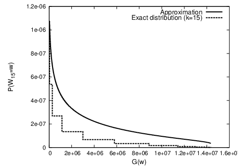
In contrast to earlier results, Corollary 4 to the LDP gives direct estimates on the guesswork distribution P⁡(G⁡(Wk)=n)P(G(W_{k})=n) for large kk, suggesting the approximation

P⁡(G⁡(Wk)=n)≈1n​exp⁡(−k​Λ∗​(k−1​log⁡n)).\displaystyle P(G(W_{k})=n)\approx\frac{1}{n}\exp(-k\Lambda^{*}(k^{-1}\log n)). (2)

As this calculation only involves the determination of Λ∗\Lambda^{*}, to approximately calculate the probability of the nthn^{\rm th} most likely word in words of length kk one does not have to identify the word itself, which would be computationally cumbersome, particularly for non-i.i.d. word sources.

Corollary 5 to the LDP recovers a rôle for Shannon entropy in the asymptotic analysis of guesswork. It shows that the scaled expectation of the logarithm of the guesswork converges to specific Shannon entropy

limk→∞1k​E​(log⁡G⁡(Wk))=limk→∞1k​H​(Wk),\displaystyle\lim_{k\to\infty}\frac{1}{k}{E}(\log G(W_{k}))=\lim_{k\to\infty}\frac{1}{k}H(W_{k}),

where

H⁡(Wk):=∑w∈𝔸kP⁡(Wk=w)​log⁡P⁡(Wk=w).\displaystyle H(W_{k}):=\sum_{w\in{\mathbb{A}}^{k}}{P}(W_{k}=w)\log{P}(W_{k}=w).

II A Large Deviation Principle

Consider the sequence of random variables {k−1​log⁡G⁡(Wk)}\{k^{-1}\log G(W_{k})\}. Our starting point is the observation that the left hand side of (1) is the scaled Cumulant Generating Function (sCGF) of this sequence:

Λ⁡(α):=limk→∞1k​log⁡E⁡(eα​log⁡G​(Wk)),\displaystyle\Lambda(\alpha):=\lim_{k\rightarrow\infty}\frac{1}{k}\log{E}\left(e^{\alpha\log G(W_{k})}\right),

which is shown to exist for α>0\alpha>0 in [2][3] and for α>−1\alpha>-1 in [4].

Assumption 1

For α>−1\alpha>-1, the sCGF Λ⁡(α)\Lambda(\alpha) exists, is equal to α\alpha times the specific Rényi entropy, and has a continuous derivative in that range.

We also assume the following regularity condition on the probability of the most likely word.

Assumption 2

The limit

g1=limk→∞1k​log⁡P⁡(G⁡(Wk)=1)\displaystyle{g_{1}}=\lim_{k\to\infty}\frac{1}{k}\log P(G(W_{k})=1) (3)

exists in (−∞,0](-\infty,0].

This assumption is transparently true for words constructed of i.i.d. or Markovian letters.

We first show that the sCGF exists everywhere.

Lemma 1 (Existence of the sCGF)

Under assumptions 1 and 2, for all α≤−1\alpha\leq-1

Λ⁡(α)=limk→∞1k​log⁡P⁡(G⁡(Wk)=1)=g1=limβ↓−1Λ⁡(β).\displaystyle\Lambda(\alpha)=\lim_{k\rightarrow\infty}\frac{1}{k}\log{P}(G(W_{k})=1)={g_{1}}=\lim_{\beta\downarrow-1}\Lambda(\beta).
Proof:

Let α≤−1\alpha\leq-1 and note that

logP(G(Wk)=1)≤log∑i=1mkP(G(Wk)=i)iα\displaystyle\log P(G(W_{k})=1)\leq\log\sum_{i=1}^{m^{k}}P(G(W_{k})=i)i^{\alpha}
=logE(eα​log⁡G​(Wk))≤logP(G(Wk)=1)+log∑i=1∞iα.\displaystyle=\log{E}\left(e^{\alpha\log G(W_{k})}\right)\leq\log P(G(W_{k})=1)+\log\sum_{i=1}^{\infty}i^{\alpha}.

Taking lim infk→∞k−1\liminf_{k\to\infty}k^{-1} with the first inequality and lim supk→∞k−1\limsup_{k\to\infty}k^{-1} with the second while using the Principle of the Largest Term, [6, Lemma 1.2.15] and usual estimates on the harmonic series, we have that

limk→∞1k​log⁡E⁡(eα​log⁡G​(Wk))=limk→∞1k​log⁡P⁡(G⁡(Wk)=1)\displaystyle\lim_{k\to\infty}\frac{1}{k}\log{E}(e^{\alpha\log G(W_{k})})=\lim_{k\to\infty}\frac{1}{k}\log P(G(W_{k})=1)

for all α≤−1\alpha\leq-1.

As Λ\Lambda is the limit of a sequence of convex functions and is finite everywhere, it is continuous and therefore limβ↓−1Λ⁡(β)=Λ⁡(−1)\lim_{\beta\downarrow-1}\Lambda(\beta)=\Lambda(-1). ∎Thus the sCGF Λ\Lambda exists and is finite for all α\alpha, with a potential discontinuity in its derivative at α=−1\alpha=-1. This discontinuity, when it exists, will have a bearing on the nature of the rate function governing the LDP for {k−1​log⁡G⁡(Wk)}\{k^{-1}\log G(W_{k})\}. Indeed, the following quantity will play a significant rôle in our results:

γ:=limα↓−1dd​α​Λ​(α).\displaystyle{\gamma}:=\lim_{\alpha\downarrow-1}\frac{d}{d\alpha}\Lambda(\alpha). (4)

We will prove that the number of words with approximately equal highest probability is close to exp⁡(k​γ)\exp(k{\gamma}). In the special case where the {Wk}\{W_{k}\} are constructed of i.i.d. letters, this is exactly true and the veracity of the following Lemma can be verified directly.

Lemma 2 (The number of most likely words)

If {Wk}\{W_{k}\} are constructed of i.i.d. letters, then

γ\displaystyle{\gamma} =limα↓−1dd​α​α​R1​((1+α)−1)\displaystyle=\lim_{\alpha\downarrow-1}\frac{d}{d\alpha}\alpha R_{1}((1+\alpha)^{-1})
=log⁡|{w:P⁡(W1=w)=P⁡(G⁡(W1)=1)}|,\displaystyle=\log|\{w:P(W_{1}=w)=P(G(W_{1})=1)\}|,

where |⋅||\cdot| indicates the number of elements in the set.

This i.i.d. result doesn’t extend directly to the non-i.i.d. case and in general Lemma 2 can only be used to establish a lower bound on γ{\gamma}:

γ=limα↓−1dd​α​Λ​(α)≥lim supk→∞limα↓−1dd​α​α​Rk​((1+α)−1),\displaystyle{\gamma}=\lim_{\alpha\downarrow-1}\frac{d}{d\alpha}\Lambda(\alpha)\geq\limsup_{k\to\infty}\lim_{\alpha\downarrow-1}\frac{d}{d\alpha}\alpha R_{k}((1+\alpha)^{-1}), (5)

e.g [7, Theorem 24.5]. This lower bound can be loose, as can be seen with the following example. Consider the sequence of distributions for some ϵ>0\epsilon>0

P⁡(Wk=i)={m−k​(1+ϵ)if ​i=1OPENm−k​(1−ϵ​(mk−1)−1))otherwise.\displaystyle P(W_{k}=i)=\begin{cases}m^{-k}(1+\epsilon)&\text{if }i=1\\ m^{-k}(1-\epsilon(m^{k}-1)^{-1}))&\text{otherwise}.\end{cases}

For each fixed kk there is one most likely word and we have log⁡(1)=0\log(1)=0 on the right hand side of equation (5) by Lemma 2. The left hand side, however, gives log⁡(m)\log(m). Regardless, this intuition guides our understanding of γ{\gamma}, but the formal statement of it approximately capturing the number of most likely words will transpire to be

g1=limk→∞1kloginf{w:G⁡(w)<exp⁡(k​γ)}P(Wk=w),\displaystyle{g_{1}}=\lim_{k\to\infty}\frac{1}{k}\log\inf_{\{w:G(w)<\exp(k{\gamma})\}}P(W_{k}=w),

where g1{g_{1}} is defined in equation (3).

We define the candidate rate function as the Legendre-Fenchel transform of the sCGF

Λ∗​(x)\displaystyle\Lambda^{*}(x) :=supα∈ℝ{x​α−Λ⁡(α)}\displaystyle:=\sup_{\alpha\in{\mathbb{R}}}\{x\alpha-\Lambda(\alpha)\}
={−x−g1 if ​x∈[0,γ]supα∈ℝ{x​α−Λ⁡(α)} if ​x∈(γ,log⁡(m)].\displaystyle=\begin{cases}-x-{g_{1}}&\text{ if }x\in[0,{\gamma}]\\ \sup_{\alpha\in{\mathbb{R}}}\{x\alpha-\Lambda(\alpha)\}&\text{ if }x\in({\gamma},\log(m)].\end{cases}

The LDP cannot be proved directly by Baldi’s version of the Gärtner-Ellis theorem [8][6, Theorem 4.5.20] as Λ∗\Lambda^{*} does not have exposing hyper-planes for x∈[0,γ]x\in[0,{\gamma}]. Instead we use a combination of that theorem with the methodology described in detail in [9] where, as our random variables are bounded 0≤k−1​log⁡G⁡(Wk)≤log⁡(m)0\leq k^{-1}\log G(W_{k})\leq\log(m), in order to prove the LDP it suffices to show that the following exist in [0,∞][0,\infty] for all x∈[0,log⁡m]x\in[0,\log m] and equals −Λ∗​(x)-\Lambda^{*}(x):

limϵ↓0lim infk→∞1k​log⁡P⁡(1k​log⁡(G⁡(Wk))∈Bϵ​(x))\displaystyle\lim_{\epsilon\downarrow 0}\liminf_{k\rightarrow\infty}\frac{1}{k}\log P\left(\frac{1}{k}\log(G(W_{k}))\in B_{\epsilon}(x)\right)
=limϵ↓0lim supk→∞1k​log⁡P⁡(1k​log⁡(G⁡(Wk))∈Bϵ​(x)),\displaystyle=\lim_{\epsilon\downarrow 0}\limsup_{k\rightarrow\infty}\frac{1}{k}\log P\left(\frac{1}{k}\log(G(W_{k}))\in B_{\epsilon}(x)\right), (6)

where Bϵ​(x)=(x−ϵ,x+ϵ)B_{\epsilon}(x)=(x-\epsilon,x+\epsilon).

Theorem 3 (The large deviations of guesswork)

Under assumptions 1 and 2, the sequence {k−1​log⁡G⁡(Wk)}\{k^{-1}\log G(W_{k})\} satisfies a LDP with rate function Λ∗\Lambda^{*}.

Proof:

To establish (6) we have separate arguments depending on xx. We divide [0,log⁡(m)][0,\log(m)] into two parts: [0,γ][0,{\gamma}] and (γ,log⁡(m)]({\gamma},\log(m)]. Baldi’s upper bound holds for any x∈[0,log⁡(m)]x\in[0,\log(m)]. Baldi’s lower bound applies for any x∈(γ,log⁡(m)]x\in({\gamma},\log(m)] as Λ∗\Lambda^{*} is continuous and, as Λ⁡(α)\Lambda(\alpha) has a continuous derivative for α>−1\alpha>-1, it only has a finite number of points without exposing hyper-planes in that region. For x∈[0,γ]x\in[0,{\gamma}], however, we need an alternate lower bound.

Consider x∈[0,γ]x\in[0,{\gamma}] and define the sets

Kk​(x,ϵ):={w∈𝔸k:k−1​log⁡G⁡(w)∈Bϵ​(x)},\displaystyle K_{k}(x,\epsilon):=\left\{w\in{\mathbb{A}}^{k}:k^{-1}\log G(w)\in B_{\epsilon}(x)\right\},

letting |Kk​(x,ϵ)||K_{k}(x,\epsilon)| denote the number of elements in each set. We have the bound

|Kk​(x,ϵ)|​infw∈Kk​(x,ϵ)P⁡(Wk=w)\displaystyle|K_{k}(x,\epsilon)|\inf_{w\in K_{k}(x,\epsilon)}{P}(W_{k}=w)
≤P⁡(1k​log⁡G⁡(Wk)∈Bϵ​(x)).\displaystyle\leq P\left(\frac{1}{k}\log G(W_{k})\in B_{\epsilon}(x)\right).

As ⌊ek⁡(x−ϵ)⌋≤|Kk​(x,ϵ)|≤⌈ek⁡(x+ϵ)⌉\lfloor e^{k(x-\epsilon)}\rfloor\leq|K_{k}(x,\epsilon)|\leq\lceil e^{k(x+\epsilon)}\rceil, we have that

x=limϵ→0limk→∞1k​log⁡|Kk​(x,ϵ)|.\displaystyle x=\lim_{\epsilon\to 0}\lim_{k\to\infty}\frac{1}{k}\log|K_{k}(x,\epsilon)|. (7)

By Baldi’s upper bound, we have that

limϵ↓0lim supk→∞1k​log⁡P⁡(1k​log⁡G⁡(Wk)∈Bϵ​(x))\displaystyle\lim_{\epsilon\downarrow 0}\limsup_{k\rightarrow\infty}\frac{1}{k}\log P\left(\frac{1}{k}\log G(W_{k})\in B_{\epsilon}(x)\right) ≤x+g1.\displaystyle\leq x+{g_{1}}.

Thus to complete the argument, for the complementary lower bound we need to show that for any x∈[0,γ]x\in[0,{\gamma}]

limϵ↓0lim infk→∞infw∈Kk​(x,ϵ)1k​log⁡P⁡(Wk=w)=g1.\displaystyle\lim_{\epsilon\downarrow 0}\liminf_{k\rightarrow\infty}\inf_{w\in K_{k}(x,\epsilon)}\frac{1}{k}\log{P}(W_{k}=w)={g_{1}}.

If Λ∗​(x)<∞\Lambda^{*}(x)<\infty for some x>γx>{\gamma}, then for ϵ>0\epsilon>0 sufficiently small let x∗x^{*} be such that Λ∗​(x∗)<∞\Lambda^{*}(x^{*})<\infty and x∗−ϵ>max⁡(γ,x+ϵ)x^{*}-\epsilon>\max({\gamma},x+\epsilon). Then by Baldi’s lower bound, which applies as x∗∈(γ,log⁡(m)]x^{*}\in({\gamma},\log(m)], we have

−infy∈Bϵ​(x∗)Λ∗(y)≤lim infk→∞1klogP(1klogG(Wk)∈Bϵ(x∗)).\displaystyle-\inf_{y\in B_{\epsilon}(x^{*})}\Lambda^{*}(y)\leq\liminf_{k\to\infty}\frac{1}{k}\log P\left(\frac{1}{k}\log G(W_{k})\in B_{\epsilon}(x^{*})\right).

Now

P⁡(1k​log⁡G⁡(Wk)∈Bϵ​(x∗))\displaystyle P\left(\frac{1}{k}\log G(W_{k})\in B_{\epsilon}(x^{*})\right)
≤|Kk​(x∗,ϵ)|​supw∈Kk​(x∗,ϵ)P⁡(Wk=w)\displaystyle\leq|K_{k}(x^{*},\epsilon)|\sup_{w\in K_{k}(x^{*},\epsilon)}{P}(W_{k}=w)
≤|Kk​(x∗,ϵ)|​infw∈Kk​(x,ϵ)P⁡(Wk=w),\displaystyle\leq|K_{k}(x^{*},\epsilon)|\inf_{w\in K_{k}(x,\epsilon)}{P}(W_{k}=w),

where in the last line we have used the monotonicity of guesswork and the fact that x∗−ϵ>x+ϵx^{*}-\epsilon>x+\epsilon. Taking lower limits and using equation (7) with |Kk​(x∗,ϵ)||K_{k}(x^{*},\epsilon)|, we have that

−infy∈Bϵ​(x∗)Λ∗(y)\displaystyle-\inf_{y\in B_{\epsilon}(x^{*})}\Lambda^{*}(y) ≤x∗+lim infk→∞infw∈Kk​(x,ϵ)1k​log⁡P⁡(Wk=w)\displaystyle\leq x^{*}+\liminf_{k\to\infty}\inf_{w\in K_{k}(x,\epsilon)}\frac{1}{k}\log{P}(W_{k}=w)

for all such x∗,xx^{*},x. Taking limits as ϵ↓0\epsilon\downarrow 0 and then limits as x∗↓γx^{*}\downarrow{\gamma} we have

−limx∗↓γΛ∗(x∗)≤γ+limϵ↓0lim infk→∞infw∈Kk​(x,ϵ)1klogP(Wk=w),\displaystyle-\lim_{x^{*}\downarrow{\gamma}}\Lambda^{*}(x^{*})\leq{\gamma}+\lim_{\epsilon\downarrow 0}\liminf_{k\rightarrow\infty}\inf_{w\in K_{k}(x,\epsilon)}\frac{1}{k}\log{P}(W_{k}=w),

but limx∗↓γΛ∗​(x∗)=−γ−g1\lim_{x^{*}\downarrow{\gamma}}\Lambda^{*}(x^{*})=-{\gamma}-{g_{1}} so that

limϵ↓0lim infk→∞infw∈Kk​(x,ϵ)1k​log⁡P⁡(Wk=w)=g1,\displaystyle\lim_{\epsilon\downarrow 0}\liminf_{k\rightarrow\infty}\inf_{w\in K_{k}(x,\epsilon)}\frac{1}{k}\log{P}(W_{k}=w)={g_{1}},

as required.

Only one case remains: if Λ∗​(x)=∞\Lambda^{*}(x)=\infty for all x>γx>{\gamma}, then we require an alternative argument to ensure that

lim infk→∞infw∈Kk​(x,ϵ)1k​log⁡P⁡(Wk=w)=g1.\displaystyle\liminf_{k\to\infty}\inf_{w\in K_{k}(x,\epsilon)}\frac{1}{k}\log{P}(W_{k}=w)={g_{1}}.

This situation happens if, in the limit, the distribution of words is near uniform on the set of all words with positive probability. Thus define

μ:=lim supk→∞1k​log⁡|{w:P⁡(Wk=w)>0}|.\displaystyle\mu:=\limsup_{k\to\infty}\frac{1}{k}\log|\{w:P(W_{k}=w)>0\}|.

As Λ∗​(x)=∞\Lambda^{*}(x)=\infty for all x>γx>{\gamma}, μ≤γ\mu\leq{\gamma}. To see γ=μ{\gamma}=\mu, note that γ=limα↓−1Λ′​(α)≤Λ′​(0){\gamma}=\lim_{\alpha\downarrow-1}\Lambda^{\prime}(\alpha)\leq\Lambda^{\prime}(0). As both Λ⁡(α)\Lambda(\alpha) and α​Rk​((1+α)−1)\alpha R_{k}((1+\alpha)^{-1}) are finite and differentiable in a neighborhood of 00, by [7, Theorem 25.7]

Λ′​(0)=limk→∞1k​dd​α​α​Rk​((1+α)−1)|α=0=limk→∞1k​H​(Wk).\displaystyle\Lambda^{\prime}(0)=\lim_{k\to\infty}\frac{1}{k}\frac{d}{d\alpha}\alpha R_{k}((1+\alpha)^{-1})|_{\alpha=0}=\lim_{k\to\infty}\frac{1}{k}H(W_{k}).

and limk→∞k−1​H​(Wk)≤μ\lim_{k\to\infty}k^{-1}H(W_{k})\leq\mu. Thus γ=μ{\gamma}=\mu and, due to convexity, Λ\Lambda is linear with slope μ\mu on α∈(−1,0]\alpha\in(-1,0]. As Λ⁡(0)=0\Lambda(0)=0, using Lemma 1 we have that g1=−μ{g_{1}}=-\mu. Let x<μx<\mu and consider

l\displaystyle{l} =lim supk→∞supw∈Kk​(x+2​ϵ,ϵ)1k​log⁡P⁡(Wk=w)\displaystyle=\limsup_{k\to\infty}\sup_{w\in K_{k}(x+2\epsilon,\epsilon)}\frac{1}{k}\log{P}(W_{k}=w)
≤lim infk→∞infw∈Kk​(x,ϵ)1k​log⁡P⁡(Wk=w).\displaystyle\leq\liminf_{k\to\infty}\inf_{w\in K_{k}(x,\epsilon)}\frac{1}{k}\log{P}(W_{k}=w).

We shall assume that l<g1{l}<{g_{1}} and show this results in a contradiction. Let ϵ<min⁡(g1−l,μ−x)/2\epsilon<\min({g_{1}}-{l},\mu-x)/2, then there exists NϵN_{\epsilon} such that

∑w∈𝔸kP⁡(Wk=w)\displaystyle\sum_{w\in{\mathbb{A}}^{k}}P(W_{k}=w) ≤ek⁡(x+ϵ)​ek⁡(g1+ϵ)+ek⁡(μ+ϵ)​ek⁡(l+ϵ)\displaystyle\leq e^{k(x+\epsilon)}e^{k({g_{1}}+\epsilon)}+e^{k(\mu+\epsilon)}e^{k({l}+\epsilon)}
=ek⁡(−μ+x+2​ϵ)+ek⁡(−g1+l+2​ϵ),\displaystyle=e^{k(-\mu+x+2\epsilon)}+e^{k(-{g_{1}}+{l}+2\epsilon)},

for all k>Nϵk>N_{\epsilon}, but this is strictly less than 11 for kk sufficiently large and thus l=g1{l}={g_{1}}. Finally, for x=μx=\mu, and ϵ>0\epsilon>0, note that we can decompose [0,log⁡(m)][0,\log(m)] into three parts, [0,μ−ϵ]∪(μ−ϵ,μ+ϵ)∪[μ+ϵ,log⁡(m)][0,\mu-\epsilon]\cup(\mu-\epsilon,\mu+\epsilon)\cup[\mu+\epsilon,\log(m)], where the scaled probability of the guesswork being in either the first or last set is decaying, but

0\displaystyle 0 =limk→∞1k​log⁡P⁡(1k​log⁡G⁡(Wk)∈[0,log⁡(m)])\displaystyle=\lim_{k\to\infty}\frac{1}{k}\log P\left(\frac{1}{k}\log G(W_{k})\in[0,\log(m)]\right)

and so the result follows from an application of the principle of the largest term.

Thus for any x∈[0,log⁡(m)]x\in[0,\log(m)],

limϵ↓0lim infk→∞1k​log⁡P⁡(1k​log⁡(G⁡(Wk))∈Bϵ​(x))\displaystyle\lim_{\epsilon\downarrow 0}\liminf_{k\rightarrow\infty}\frac{1}{k}\log P\left(\frac{1}{k}\log(G(W_{k}))\in B_{\epsilon}(x)\right)
=limϵ↓0lim supk→∞1k​log⁡P⁡(1k​log⁡(G⁡(Wk))∈Bϵ​(x))\displaystyle=\lim_{\epsilon\downarrow 0}\limsup_{k\rightarrow\infty}\frac{1}{k}\log P\left(\frac{1}{k}\log(G(W_{k}))\in B_{\epsilon}(x)\right)
=−Λ∗​(x)\displaystyle=-\Lambda^{*}(x)

and the LDP is proved. ∎

In establishing the LDP, we have shown that any rate function that governs such an LDP must have the form of a straight line in [0,γ][0,{\gamma}] followed by a strictly convex function. The initial straight line comes from all words that are, in an asymptotic sense, of greatest likelihood.

While the LDP is for the sequence {k−1​log⁡G⁡(Wk)}\{k^{-1}\log G(W_{k})\}, it can be used to develop the more valuable direct estimate of the distribution of each G⁡(Wk)G(W_{k}) found in equation (2). The next corollary provides a rigorous statement, but an intuitive, non-rigorous argument for understanding the result therein is that from the LDP we have the approximation that for large kk

d​P​(1k​log⁡G⁡(Wk)=x)≈exp⁡(−k​Λ∗​(x)).\displaystyle dP\left(\frac{1}{k}\log G(W_{k})=x\right)\approx\exp(-k\Lambda^{*}(x)).

As for large kk the distribution of k−1​log⁡G⁡(Wk)k^{-1}\log G(W_{k}) and G⁡(Wk)/kG(W_{k})/k are ever closer to having densities, using the change of variables formula gives

d​P​(1k​G​(Wk)=x)\displaystyle dP\left(\frac{1}{k}G(W_{k})=x\right) =1k​x​d​P​(1k​log⁡G⁡(Wk)=x)\displaystyle=\frac{1}{kx}dP\left(\frac{1}{k}\log G(W_{k})=x\right)
≈1k​x​exp⁡(−k​Λ∗​(1k​log⁡(k​x))).\displaystyle\approx\frac{1}{kx}\exp\left(-k\Lambda^{*}\left(\frac{1}{k}\log(kx)\right)\right).

Finally, the substitution k​x=nkx=n gives the approximation in equation (2). To make this heuristic precise requires distinct means, explained in the following corollary.

Corollary 4 (Direct estimates on guesswork)

Recall the definition

Kk​(x,ϵ):={w∈𝔸k:k−1​log⁡G⁡(w)∈Bϵ​(x)}.\displaystyle K_{k}(x,\epsilon):=\left\{w\in{\mathbb{A}}^{k}:k^{-1}\log G(w)\in B_{\epsilon}(x)\right\}.

For any x∈[0,log⁡(m)]x\in[0,\log(m)] we have

limϵ↓0lim infk→∞1k​log​infw∈Kk​(x,ϵ)P⁡(Wk=w)\displaystyle\lim_{\epsilon\downarrow 0}\liminf_{k\rightarrow\infty}\frac{1}{k}\log\inf_{w\in K_{k}(x,\epsilon)}{P}(W_{k}=w)
=limϵ↓0lim supk→∞1k​log​supw∈Kk​(x,ϵ)P⁡(Wk=w)\displaystyle=\lim_{\epsilon\downarrow 0}\limsup_{k\rightarrow\infty}\frac{1}{k}\log\sup_{w\in K_{k}(x,\epsilon)}{P}(W_{k}=w)
=−(x+Λ∗​(x)).\displaystyle=-\left(x+\Lambda^{*}(x)\right).
Proof:

We show how to prove the upper bound as the lower bound follows using analogous arguments, as do the edge cases. Let x∈(0,log⁡(m))x\in(0,\log(m)) and ϵ>0\epsilon>0 be given. Using the monotonicity of guesswork

lim supk→∞1k​log​supw∈Kk​(x,ϵ)P⁡(Wk=w)\displaystyle\limsup_{k\to\infty}\frac{1}{k}\log\sup_{w\in K_{k}(x,\epsilon)}{P}(W_{k}=w)
≤lim infk→∞1k​log​infw∈Kk​(x−2​ϵ,ϵ)P⁡(Wk=w).\displaystyle\leq\liminf_{k\to\infty}\frac{1}{k}\log\inf_{w\in K_{k}(x-2\epsilon,\epsilon)}{P}(W_{k}=w).

Using the estimate found in Theorem 3 and the LDP provides an upper bound on the latter:

(x−3​ϵ)+lim infk→∞1k​log​infw∈Kk​(x−2​ϵ,ϵ)P⁡(Wk=w)\displaystyle(x-3\epsilon)+\liminf_{k\to\infty}\frac{1}{k}\log\inf_{w\in K_{k}(x-2\epsilon,\epsilon)}{P}(W_{k}=w)
≤lim infk→∞1k​log⁡P⁡(1k​log⁡(G⁡(Wk))∈Bϵ​(x−2​ϵ))\displaystyle\leq\liminf_{k\to\infty}\frac{1}{k}\log P\left(\frac{1}{k}\log(G(W_{k}))\in B_{\epsilon}(x-2\epsilon)\right)
≤lim supk→∞1k​log⁡P⁡(1k​log⁡(G⁡(Wk))∈[x−3​ϵ,x−ϵ])\displaystyle\leq\limsup_{k\to\infty}\frac{1}{k}\log P\left(\frac{1}{k}\log(G(W_{k}))\in[x-3\epsilon,x-\epsilon]\right)
≤−infx∈[x−3​ϵ,x−ϵ]Λ∗(x).\displaystyle\leq-\inf_{x\in[x-3\epsilon,x-\epsilon]}\Lambda^{*}(x).

Thus

lim supk→∞1k​log​supw∈Kk​(x,ϵ)P⁡(Wk=w)\displaystyle\limsup_{k\to\infty}\frac{1}{k}\log\sup_{w\in K_{k}(x,\epsilon)}{P}(W_{k}=w)
≤−x+3​ϵ−infx∈[x−3​ϵ,x−ϵ]Λ∗​(x).\displaystyle\leq-x+3\epsilon-\inf_{x\in[x-3\epsilon,x-\epsilon]}\Lambda^{*}(x).

Thus the upper-bound follows taking ϵ↓0\epsilon\downarrow 0 and using the continuity when finite of Λ∗\Lambda^{*}. ∎

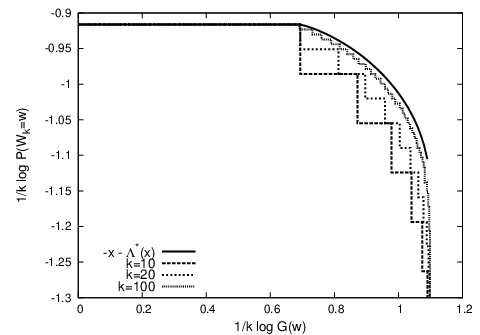
Unpeeling limits, this corollary shows that when kk is large the probability of the nthn^{\rm th} most likely word is approximately 1/n​exp⁡(−k​Λ∗​(k−1​log⁡n))1/n\exp(-k\Lambda^{*}(k^{-1}\log n)), without the need to identify the word itself. This justifies the approximation in equation (2), whose complexity of evaluation does not depend on kk. We demonstrate its merit by example in Section III.

Before that, as a corollary to the LDP we find the following rôle for the specific Shannon entropy. Thus, although Massey established that for a given word length the Shannon entropy is only a lower bound on the guesswork, for growing password length the specific Shannon entropy determines the linear growth rate of the expectation of the logarithm of guesswork.

Corollary 5 (Shannon entropy and guesswork)

Under assumptions 1 and 2,

limk→∞1k​E​(log⁡G⁡(Wk))=limk→∞1k​H​(Wk),\displaystyle\lim_{k\rightarrow\infty}\frac{1}{k}{E}(\log G(W_{k}))=\lim_{k\to\infty}\frac{1}{k}H(W_{k}),

the specific Shannon entropy.

Proof:

Note that Λ∗​(x)=0\Lambda^{*}(x)=0 if and only if x=Λ′​(0)=limk−1​H​(Wk)x=\Lambda^{\prime}(0)=\lim k^{-1}H(W_{k}), by arguments found in the proof of Theorem 3. The weak law then follows by concentration of measure, e.g. [10]. ∎

III Examples

I.i.d letters.

Refer to caption
Fig. 1: Illustration of Corollary 4. Words constructed from i.i.d letters with P⁡(W1=1)=0.4,P⁡(W1=2)=0.4,P⁡(W1=3)=0.2P(W_{1}=1)=0.4,P(W_{1}=2)=0.4,P(W_{1}=3)=0.2. For k=15k=15 comparison of the probability of nthn^{\rm th} most likely word and the approximation 1/n​exp⁡(−k​Λ∗​(k−1​log⁡n))1/n\exp(-k\Lambda^{*}(k^{-1}\log n)) versus n∈{1,…,315}n\in\{1,\ldots,3^{15}\}.
Refer to caption
Fig. 2: Illustration of Corollary 4. Words constructed from i.i.d letters with P⁡(W1=1)=0.4,P⁡(W1=2)=0.4,P⁡(W1=3)=0.2P(W_{1}=1)=0.4,P(W_{1}=2)=0.4,P(W_{1}=3)=0.2. For k=10,20k=10,20 and 100100, comparison of k−1k^{-1} times the logarithm of the probability of nthn^{\rm th} most likely word versus k−1k^{-1} times the logarithm of nn, as well as the approximation −x−Λ∗​(x)-x-\Lambda^{*}(x) versus xx.

Assume words are constructed of i.i.d. letters. Let W1W_{1} take values in 𝔸={1,…,m}{\mathbb{A}}=\{1,\ldots,m\} and assume P⁡(W1=i)≥P⁡(W1=j){P}(W_{1}=i)\geq{P}(W_{1}=j) if i≤ji\leq j. Then from [2, 4] and Lemma 1 we have that

Λ⁡(α)={(1+α)​log​∑w∈𝔸P​(W1=w)1/(1+α)if ​α>−1log⁡P⁡(W1=1)if ​α≤−1.\displaystyle\Lambda(\alpha)=\begin{cases}\displaystyle(1+\alpha)\log\sum_{w\in{\mathbb{A}}}P(W_{1}=w)^{1/(1+\alpha)}&\text{if }\alpha>-1\\ \log{P}(W_{1}=1)&\text{if }\alpha\leq-1.\end{cases}

From Lemma 2 we have that

γ=limα↓−1Λ′​(α)∈{0,log⁡(2),…,log⁡(m)}\displaystyle{\gamma}=\lim_{\alpha\downarrow-1}\Lambda^{\prime}(\alpha)\in\{0,\log(2),\ldots,\log(m)\}

and no other values are possible. Unless the distribution of W1W_{1} is uniform, Λ∗​(x)\Lambda^{*}(x) does not have a closed form for all xx, but is readily calculated numerically. With |𝔸|=3|{\mathbb{A}}|=3 and k=15k=15, Figure 1 compares the exact distribution P⁡(Wk=w)P(W_{k}=w) versus G⁡(w)G(w) with the approximation found in equation (2). As there are 315≈1.43^{15}\approx 1.4 million words, the likelihood of any one word is tiny, but the quality of the approximation can clearly be seen. Rescaling the guesswork and probabilities to make them comparable for distinct kk, Figure 2 illustrates the quality of the approximation as kk grows. By k=100k=100 there are 3100≈5.13^{100}\approx 5.1 times 104710^{47} words and the underlying combinatorial complexities of the explicit calculation become immense, yet the complexity of calculating the approximation has not increased.

Markovian letters.

Refer to caption
Fig. 3: Illustration of rate functions in Theorem 3. Words constructed from Markov letters on |𝔸|=2|{\mathbb{A}}|=2. Three rate functions illustrating only values of γ{\gamma} possible, log⁡(1)\log(1), log⁡(ϕ)≈0.48\log(\phi)\approx 0.48 and log⁡(2)\log(2), from Lemma 6.

As an example of words constructed of correlated letters, consider {Wk}\{W_{k}\} where the letters are chosen via a process a Markov chain with transition matrix PP and some initial distribution on |𝔸|=2|{\mathbb{A}}|=2. Define the matrix PαP_{\alpha} by (Pα)i,j=pi,j1/(1+α)(P_{\alpha})_{i,j}=p_{i,j}^{1/(1+\alpha)}, then by [3, 4] and Lemma 1 we have that

Λ⁡(α)={(1+α)​log⁡ρ⁡(Pα)if ​α>−1log⁡max⁡(p1,1,p2,2,p1,2​p2,1)if ​α≤−1,\displaystyle\Lambda(\alpha)=\begin{cases}(1+\alpha)\log\rho(P_{\alpha})&\text{if }\alpha>-1\\ \log\max(p_{1,1},p_{2,2},\sqrt{p_{1,2}\,p_{2,1}})&\text{if }\alpha\leq-1,\end{cases}

where ρ\rho is the spectral radius operator. In the two letter alphabet case, with β=1/(1+α)\beta=1/(1+\alpha) we have that ρ⁡(P(1−β)/β)\rho(P_{(1-\beta)/\beta}) equals

p1,1β+p2,2β2+(p1,1β−p2,2β)2+4​(1−p2,2)β​(1−p1,1)β2.\displaystyle\frac{p_{1,1}^{\beta}+p_{2,2}^{\beta}}{2}+\frac{\sqrt{(p_{1,1}^{\beta}-p_{2,2}^{\beta})^{2}+4(1-p_{2,2})^{\beta}(1-p_{1,1})^{\beta}}}{2}.

As with the i.i.d. letters example, apart from in special cases, the rate function Λ∗\Lambda^{*} cannot be calculated in closed form, but is readily evaluated numerically. Regardless, we have the following, perhaps surprising, result on the exponential rate of growth of the size of the set of almost most likely words.

Lemma 6 (The Golden Ratio and Markovian letters)

For {Wk}\{W_{k}\} constructed of Markovian letters,

γ=limα↓−1Λ′​(α)∈{0,log⁡(ϕ),log⁡(2)},\displaystyle{\gamma}=\lim_{\alpha\downarrow-1}\Lambda^{\prime}(\alpha)\in\{0,\log(\phi),\log(2)\},

where ϕ=(1+5)/2\phi=(1+\sqrt{5})/2 is the Golden Ratio, and no other values are possible.

This lemma can be proved by directly evaluating the derivative of Λ⁡(α)\Lambda(\alpha) with respect to α\alpha. Note that here exp⁡(k​γ)\exp(k{\gamma}) definitely only describes the number of words of equal highest likelihood when kk is large as the initial distribution of the Markov chain plays no rôle in γ{\gamma}’s evaluation.

The case where γ=log⁡(2){\gamma}=\log(2) occurs when p1,1=p2,2=1/2p_{1,1}=p_{2,2}=1/2. The most interesting case is when there are approximately ϕk\phi^{k} approximately equally most likely words. This occurs if p1,1=p1,2​p2,1>p2,2p_{1,1}=\sqrt{p_{1,2}p_{2,1}}>p_{2,2}. For large kk, words of near-maximal probability have the form of a sequence of 1s, where a 2 can be inserted anywhere so long as there is a 1 between it and any other 2s. A further sub-exponential number of aberrations are allowed in any given sequence. For example, with an equiprobable initial distribution and k=4k=4 there are 88 most likely words (1111, 1112, 1121, 1211, 1212, 2111, 2121, 2112) and ϕ4≈6.86\phi^{4}\approx 6.86.

Figure 3 gives plots of Λ∗​(x)\Lambda^{*}(x) versus xx illustrating the full range of possible shapes that rate functions can take: linear, linear then strictly convex, or strictly convex, based on the transition matrices

(0.50.50.50.5),(0.60.40.90.1)​ and ​(0.850.150.150.85)\displaystyle\left(\begin{matrix}0.5&0.5\\ 0.5&0.5\end{matrix}\right),\left(\begin{matrix}0.6&0.4\\ 0.9&0.1\end{matrix}\right)\text{ and }\left(\begin{matrix}0.85&0.15\\ 0.15&0.85\end{matrix}\right)

respectively.

References

  • [1] J. L. Massey, “Guessing and entropy,” Proc. IEEE Int. Symp. Inf. Theory, pp. 204–204, 1994.
  • [2] E. Arikan, “An inequality on guessing and its application to sequential decoding,” IEEE Trans, Inf. Theory, vol. 42, pp. 525–526, 1996.
  • [3] D. Malone and W. G. Sullivan, “Guesswork and entropy,” IEEE Trans. Inf. Theory, vol. 50, no. 4, pp. 525–526, 2004.
  • [4] C.-E. Pfister and W. G. Sullivan, “Rényi entropy, guesswork moments and large deviations,” IEEE Trans. Inf. Theory, vol. 50, no. 11, pp. 2794–2800, 2004.
  • [5] M. K. Hanawal and R. Sundaresan, “Guessing revisited: A large deviations approach,” IEEE Trans. Inf. Theory, vol. 57, no. 1, pp. 70–78, 2011.
  • [6] A. Dembo and O. Zeitouni, Large Deviations Techniques and Applications. Springer, 2009.
  • [7] R. T. Rockafellar, Convex analysis, ser. Princeton Mathematical Series, No. 28. Princeton, N.J.: Princeton University Press, 1970.
  • [8] P. Baldi, “Large deviations and stochastic homogenization,” Ann. Mat. Pura Appl. (4), vol. 151, pp. 161–177, 1988.
  • [9] J. T. Lewis and C.-E. Pfister, “Thermodynamic probability theory: some aspects of large deviations,” Russian Math. Surveys, vol. 50, no. 2, pp. 279–317, 1995.
  • [10] J. T. Lewis, C.-E. Pfister, and W. G. Sullivan, “Entropy, concentration of probability and conditional limit theorems,” Markov Process. Related Fields, vol. 1, no. 3, pp. 319–386, 1995.