Variance Optimal Hedging for discrete time processes with independent increments.
Application to Electricity Markets

Stéphane GOUTTE , Nadia OUDJANE ^* and Francesco RUSSO ^†^†thanks: Luiss Guido Carli - Libera Università Internazionale degli Studi Sociali Guido Carli di Roma^†^†thanks: EDF R&D, Université Paris 13, FiME (Laboratoire de Finance des Marchés de l’Energie (Dauphine, CREST, EDF R&D) www.fime-lab.org). E-mail:nadia.oudjane@edf.fr ^†^†thanks: INRIA Rocquencourt and Cermics Ecole des Ponts, Projet MATHFI. E-mail:francesco.russo@ensta-paristech.fr Note: Université Paris 13, Mathématiques LAGA, Institut Galilée, 99 Av. J.B. Clément 93430 Villetaneuse. E-mail:goutte@math.jussieu.fr Note: ENSTA ParisTech, UMA, Unité de Mathématiques appliquées, 32 Bd. Victor, F-75739 Paris Cedex 15 (France)

October 18th 2011

Abstract

We consider the discretized version of a (continuous-time) two-factor model introduced by Benth and coauthors for the electricity markets. For this model, the underlying is the exponent of a sum of independent random variables. We provide and test an algorithm, which is based on the celebrated Föllmer-Schweizer decomposition for solving the mean-variance hedging problem. In particular, we establish that decomposition explicitly, for a large class of vanilla contingent claims. Interest is devoted in the choice of rebalancing dates and its impact on the hedging error, regarding the payoff regularity and the non stationarity of the log-price process.

Key words: Variance-optimal hedging, Föllmer-Schweizer decomposition, Lévy process, Cumulative generating function, Characteristic function, Normal Inverse Gaussian distribution, Electricity markets, Incomplete Markets, Processes with independent increments, trading dates optimization.

2010 AMS-classification: 60G50, 60G51, 91G10, 60J05, 62M99

JEL-classification: C02, C15, G11, G12, G13

1 Introduction

It is well known that the classical Black-Scholes model does not allow in real applications to replicate perfectly contingent claims. Of course, this is due to market incompleteness and specifically two major reasons : the non-Gaussianity of prices log-returns and the finite number of trading dates. The impact of these features have been intensively studied separately in the literature.

There is a large literature on pricing and hedging with non Gaussian models (allowing for stochastic volatility or jumps), in a continuous time setup. Then, the hedging error related to the discretization of the hedging strategy is in general ignored or investigated separately. One popular approach is the Variance-Optimal hedging. Let $S^{c}$ denotes the underlying price process where the superscript $c$ refers to the continuous time setting); if $H$ denotes the payoff of the option, the goal is to minimize the mean squared hedging error

\mathbb{E}[(V_{T}-H)^{2}]\quad\textrm{with}\quad V_{T}=c+\int_{0}^{T}v_{t}dS^{c}_{t}\ .

over all initial endowments $c\in\mathbb{R}$ and all (in some sense) admissible strategies $v$ . The first paper specifically on this subject is due to Duffie and Richardson, see [18]. Among significant early contributions there are [36, 37, 39, 33, 25], a fairly complete recent article on the structure of mean-variance hedging, with a rich bibliography is provided by [11]. One of the now classical tools is the so called Föllmer-Schweizer decomposition. Given a square integrable r.v. $H$ and an $({\cal F}_{t})$ -semimartingale $S=(S_{t})_{t\geq 0}$ , that decomposition consists in finding a triple $(H_{0},\xi,L)$ where $H_{0}$ is ${\cal F}_{0}$ -measurable, $\xi$ is $({\cal F}_{t})$ -predictable and $L$ is a martingale being orthogonal to the martingale part $M$ of $S$ such that $H=H_{0}+\int_{0}^{T}\xi_{s}dS_{s}+L_{T}$ . In the recent years, some attention was focused on finding explicit or quasi explicit formulae for the Föllmer-Schweizer decomposition or the optimal strategy for the mean-variance hedging problem. For instance [6] gave an expression based on Clark-Ocone type decompositions related to Lévy type measures when the underlying is a Lévy martingale, [15] still in the martingale case with techniques of partial integro differential equations. [29] obtained significant explicit decompositions when the underlying is the exponential of a Lévy process and the contingent claim is a vanilla type option appearing as some generalized Laplace transform of a finite complex measure. Other significant semi-explicit formulae appear in [30, 31]. [29] was continued by [28] in the framework of processes with independent increments with some applications to the electricity market.

However, in practice, the hedging strategy cannot be implemented continuously and the resulting optimal strategy has to be discretized. Hence, to be really relevant the hedging error should take into account this further approximation.

An alternative approach, less investigated in the literature, is to consider directly the hedging problem in discrete time as proposed by Cox Ross and Rubinstein [16]. The first incomplete market analysis in the spirit of minimizing a quadratic risk is due to [19]. They worked with the so-called local risk-minimization. The problem of Variance-Optimal hedging in the discrete time setup was proposed in [35, 38]. In the recent years some interest on discrete time was rediscovered in [8, 9, 32]. [12] revisits the seminal paper [19] in the spirit of global risk minimization. In the discrete-time context, a significant role was played by the analogous of the previously mentioned FS-decomposition. It is recalled in Definition 2.8.

Recently, many approaches have been proposed to obtain explicit or quasi-explicit formulae for computing both the variance optimal trading strategies and hedging errors in discrete time. For instance, in [1], Angelini and Herzel derive closed formulae for the variance optimal hedge ratio and the corresponding hedging error variance when the underlying asset is a geometric Brownian motion which is martingale. As we said, Kallsen and co-authors contributed at providing semi-explicit formulae for the Variance-Optimal hedging problem both in discrete and continuous time, for various kind of models. In particular in [29], semi-explicit formula are derived for the (discrete and continuous time) Variance-Optimal hedging strategy and for the resulting hedging error, in the specific case where the logarithm of the underlying price is a process with stationary independent increments. One major idea proposed in [29] and [10] consists in expressing the payoff as a linear combination of exponential payoffs for which the variance optimal hedging strategy can be expressed explicitly. With a similar methodology and in the same setting, Angelini and Herzel [2] determine the Laplace transform of the variance of the error produced by a standard delta hedging strategy when applied to several class of models. In [17] similar results are provided in the continuous time setup. In this paper, we use the generalized Laplace transform approach to extend the results of [29] to the case of processes with independent increments (PII) relaxing the stationary assumption on log-returns. The semi-explicit discrete Föllmer-Schweizer decomposition is stated in Proposition 3.11, the solution to the mean-variance hedging problem in Theorem 4.1. The expression of the quadratic hedging error in Theorem 4.3 gives a priori a criterion of market completeness as far as vanilla options are concerned. This confirms that the (even not stationary) binomial model is complete, see Proposition 4.5.

Our discrete time model consists in fact in the discretization of continuous time models which are exponentials of processes of independent increments. Given a continuous-time model $(S_{t}^{c})_{t\geq 0}$ , where $S^{c}_{t}=s_{0}\exp(X^{c}_{t})$ and $X^{c}$ is a process with independent increments and discrete trading dates $t_{0},t_{1},\cdots,t_{N}$ , our discrete model will be $S=(S_{k})$ , such that $S_{k}=S^{c}_{t_{k}}$ , for all $k=0,1,\cdots N$ . In this discrete time setting, the Variance-Optimal pricing and hedging problem consists in looking for the initial endowments $c\in\mathbb{R}$ and the admissible strategy $v=(v_{k})$ which minimizes

\mathbb{E}[(V^{N}_{T}-H)^{2}]\quad\textrm{with}\quad V^{N}_{T}=c+\sum_{k=1}^{N}v_{k}\Delta S_{k}\ .

This framework is indeed well suited to take into account together both the non-Gaussianity of log-returns and hedging errors due to the discreteness of trading times. Our investigation for quasi-explicit formulae when the underlying is the exponential of sums of independent random variables is due to two reasons.

1.

The first one comes from the fact that the basic continuous time model can be time-inhomogeneous in a natural way, see for instance [28].
2.

The second, more original reason, is that the discretized times, which correspond in our case to the rebalancing dates, are not necessarily uniformly chosen.

About item 1., some prices exhibit non stationary and non-Gaussian log-returns. One common example of this phenomenon can be observed on electricity futures or forward market: the forward volatility increases when the time to delivery decreases whereas the tails of log-returns distribution get heavier resulting in huge spikes on the Spot. The exponential Lévy factor model, proposed in [7] and [13] allows to represent both the volatility term structure and the spikes on the short term. More precisely, the forward price given at time $t$ for delivery of 1MWh at time $T_{d}\geq t$ , denoted $F_{t}^{T_{d}}$ is then modeled by a two factors model, such that

S_{t}^{c}:=F_{t}^{T_{d}}=F_{0}^{T_{d}}\exp(m_{t}^{T_{d}}+\int_{0}^{t}\sigma_{S}e^{-\lambda({T_{d}}-u)}d\Lambda_{u}+\sigma_{L}W_{t})\ ,\quad\textrm{for all}\ t\in[0,{T_{d}}]\ ,

(1.1)

where $m$ is a real deterministic trend, $\Lambda$ a real Lévy process and $W$ a real Brownian motion. Hence, forward prices are modeled as exponentials of PII with non-stationary increments and existing results from [29] valid for stationary independent processes cannot be applied for that kind of models.

Concerning item 2., the announced motivation for our development is to be able to analyze the impact of a non-homogeneous discretization of the trading dates on the Variance-Optimal hedging error. The issue of considering non-homogeneous trading dates was first considered by Geiss [21] who analyzed the impact on the hedging error of discretizing a continuously rebalanced hedging portfolio. He showed that for a given irregular payoff (e.g. a digital call), concentrating rebalancing dates near the maturity instead of rebalancing regularly can improve the convergence rate of the hedging error. Later, Geiss and Geiss [22] introduced the so called fractional smoothness quantifying the impact of the payoff irregularity on the optimal discretization grid. The reader can consult [23] for a nice survey on this subject and [24] for some recent developments.

Hence, it seems to be of real interest to be able to consider such non-homogeneous grids. However, if the continuous time log-price model $X^{c}=\log(S^{c})-\log(s_{0})$ has independent and stationary increments, considering non-homogeneous trading dates involves a non stationary discrete time process $X$ such that $X_{k}=X^{c}_{t_{k}}$ for $k=0,\cdots N$ , where $t_{0},t_{1},\cdots,t_{N}$ denote the non-homogeneous trading dates. Hence, here again existing results from [29] cannot be applied neither for hedging at non-homogeneous times nor for evaluating the resulting hedging error.

In the present work, we have performed some numerical tests concerning both applications. One major observation is the remarkable robustness of the Black-Scholes strategy that still achieves quasi-minimal hedging errors variances, with both non Gaussian log-returns and discrete rebalancing dates. Besides, our tests show that when hedging with electricity forward contracts, the impact of the choice of the rebalancing dates on the hedging error seems to be more important than the choice of log-returns distribution (Gaussian or Normal Inverse Gaussian, in our case). Concerning the case of hedging an irregular payoff (a digital call, in our case), our numerical tests confirm the result of [21]. In almost Gaussian cases, we observe that the variance optimal hedging error, can be noticeably reduced by optimizing the rebalancing dates. However, this phenomena is less pronounced when the tails of the log-returns distribution get heavier for which the hedging error gets less sensitive to the rebalancing grid. This suggests that the result of [21] and [24] could not be extended straightforwardly to the non Gaussian case.

This article is organized as follows. In Section 2, notations and generalities on the discrete Föllmer-Schweizer decomposition are presented. In Section 3, we derive semi-explicit Föllmer-Schweizer decomposition for exponential of PII. Section 4 is devoted to the solution to the global minimization problem. Illustrative example and simulation results are given in Section 5; in particular, subsection 5.2 is concerned with data coming from the electricity market.

2 Generalities and Discrete Föllmer-Schweizer decomposition

We present the context of the problem studied by [38].

Let $(\Omega,\mathcal{F},P)$ be a probability space, $N\in\mathbb{N}^{*}$ a fixed natural number and $\mathbb{F}=(\mathcal{F}_{k})_{k=0,\cdots,N}$ a fixed reference filtration. We shall assume that $\mathcal{F}=\mathcal{F}_{N}$ . Let $(S_{k})_{k=0,\cdots,N}$ be a real-valued, $\mathbb{F}$ -adapted, square-integrable process. We denote by $\Delta S_{k}$ the increments $S_{k}-S_{k-1}$ , for $k=1,\cdots,N$ . We use the convention that a sum (respectively product) over an empty set is zero (resp. one).

Definition 2.1.

We denote by $\Theta$ the set of all predictable processes $v$ (i.e.: $v_{k}$ is $\mathcal{F}_{k-1}$ -measurable for each $k\geq 1$ ) such that $v_{k}\Delta S_{k}\in{\cal L}^{2}(\Omega)$ for $k=1,\cdots,N$ . For $v\in\Theta$ , $G(v)$ is the process defined by

G_{k}(v):=\sum_{j=1}^{k}v_{j}\Delta S_{j},\quad{\rm for}\quad\ k=1,\cdots,N.

The problem addressed in [38] is the following.
Given $H\in\mathcal{L}^{2}(\Omega)$ , we look for $(V_{0}^{*},\varphi^{*})$ which minimize the quantity

\displaystyle\mathbb{E}\left[\left(H-V_{0}-G_{T}(\varphi)\right)^{2}\right]\ ,

(2.2)

over $V_{0}\in\mathbb{R}$ and $\varphi\in\Theta$ . It will be called discrete time optimization problem. The expression $\mathbb{E}\left[\left(H-V_{0}^{*}-G_{T}(\varphi^{*})\right)^{2}\right]$ will be called the variance optimal hedging error.

Definition 2.2.

Schweizer [38] introduces the following non-degeneracy condition (ND). We say that S satisfies the non-degeneracy condition (ND) if there exists a constant $\delta\in]0,1[$ such that

\displaystyle\left(\mathbb{E}[\Delta S_{k}|\mathcal{F}_{k-1}]\right)^{2}\leq\delta\mathbb{E}[(\Delta S_{k})^{2}|\mathcal{F}_{k-1}]\ ,

P.a.s for $k=1,\cdots,N$ .

Remark 2.3.

1.

If $(S_{k})$ is a martingale then (ND) is always verified.
2.

Note that by Jensen’s inequality, we always have $\left(\mathbb{E}[\Delta S_{k}|\mathcal{F}_{k-1}]\right)^{2}\leq\mathbb{E}[(\Delta S_{k})^{2}|\mathcal{F}_{k-1}]\quad{\rm a.s.}$ The point of condition (ND) is to ensure a strict inequality uniformly in $\omega$ .

To obtain another formulation of (ND), we now express $S$ in its Doob decomposition as $S_{k}=M_{k}+A_{k}$ where $M_{k}$ is a square-integrable martingale and $A_{k}$ is a square-integrable predictable process with $A_{0}=0$ . It is well-known that this decomposition is unique and is given through

\Delta A_{k}:=\mathbb{E}[\Delta S_{k}|\mathcal{F}_{k-1}]\ ,\quad\textrm{and}\quad\Delta M_{k}:=\Delta S_{k}-\Delta A_{k}\ .

We will operate with the help of some conditional moments and conditional variance setting

Var[\Delta S_{k}|\mathcal{F}_{k-1}]:=\mathbb{E}[(\Delta S_{k})^{2}|\mathcal{F}_{k-1}]-\mathbb{E}[\Delta S_{k}|\mathcal{F}_{k-1}]^{2}\ .

Remark 2.4.

For $k=1,\ldots,N$ , we have the following.

1.

$\mathbb{E}[(\Delta S_{k})^{2}|\mathcal{F}_{k-1}]=\mathbb{E}[(\Delta M_{k})^{2}|\mathcal{F}_{k-1}]+(\Delta A_{k})^{2}\ ;$
2.

$Var[\Delta S_{k}|\mathcal{F}_{k-1}]=\mathbb{E}[(\Delta M_{k})^{2}|\mathcal{F}_{k-1}]\ ;$
3.

Previous conditional variance vanishes if and only if $\Delta M_{k}=0\$ a.s.

We introduce the predictable process $\lambda_{k}$ by

\lambda_{k}:=\frac{\Delta A_{k}}{\mathbb{E}[(\Delta S_{k})^{2}|\mathcal{F}_{k-1}]}=\frac{\mathbb{E}[\Delta S_{k}|\mathcal{F}_{k-1}]}{\mathbb{E}[(\Delta S_{k})^{2}|\mathcal{F}_{k-1}]}\ ,

(2.3)

for all $k=1,\cdots,N$ . These quantities could be theoretically infinite.

Remark 2.5.

Suppose that $P(\Delta S_{k}=0)=0$ for any $k=1,\cdots,N$ .

1.

Then $\mathbb{E}[(\Delta S_{k})^{2}|\mathcal{F}_{k-1}]>0$ a.s. In fact, let $B=\{\omega|\mathbb{E}[(\Delta S_{k})^{2}(\omega)|\mathcal{F}_{k-1}]=0\}$ . This implies $\Delta A_{k}=0$ on $B$ because of Remark 2.4 1. By the same Remark,

$0=1_{B}\mathbb{E}[(\Delta M_{k})^{2}|\mathcal{F}_{k-1}]=\mathbb{E}[1_{B}(\Delta M_{k})^{2}|\mathcal{F}_{k-1}]\ ,$

so $\Delta M_{k}=0$ a.s. on $B$ . This implies that $\Delta S_{k}=0$ a.s. on $B$ . By assumption, $B$ is forced to be a null set.
2.

Previous point 1. guarantees in particular that $(\lambda_{k})$ are all finite.

Definition 2.6.

The mean-variance tradeoff process of $S$ is defined by

K^{d}_{j}:=\sum_{l=1}^{j}\frac{\mathbb{E}[\Delta S_{l}|\mathcal{F}_{l-1}]^{2}}{Var[\Delta S_{l}|\mathcal{F}_{l-1}]}\ ,

for all $j=1,\cdots,N$ . $K^{d}$ is the discrete version of the continuous time corresponding process $K$ defined for instance in Definition 2.11 of [28] or in Section 1. of [36].

Proposition 2.7.

The condition (ND) is fulfilled if and only if

\displaystyle\frac{\mathbb{E}[\Delta S_{k}|\mathcal{F}_{k-1}]^{2}}{Var[\Delta S_{k}|\mathcal{F}_{k-1}]}

is a.s. bounded uniformly in $\omega$ and k.

Proof.

See (1.6) in [38]. ∎

A basic tool for solving the optimization problem (2.2) in [38] is the discrete Föllmer-Schweizer decomposition.

Definition 2.8.

Denote by $S=M+A$ the Doob decomposition of $S$ into a martingale $M$ and a predictable process $A$ . A complex-valued square integrable random variable $H$ is said to admit a discrete Föllmer-Schweizer decomposition (or simply discrete FS-decomposition) if there exists a $\mathcal{F}_{0}$ -measurable $H_{0}$ , a complex-valued process $\xi$ such that both $Re\xi(z),Im\xi(z)$ belong to $\Theta$ , and a square integrable $\mathbb{C}$ -valued martingale $L^{H}$ such that

1.

$L^{H}M$ is a martingale;
2.

$E(L_{0}^{H})=0$ ,
3.

$H=H_{0}+\sum_{k=1}^{N}\xi_{k}\Delta S_{k}+L_{N}^{H}$ .

When Point 1. is fulfilled $L^{H}$ and $M$ are called strongly orthogonal.
If $H$ is a real valued r.v. then $H$ admits a real discrete FS decomposition if it admits a FS decomposition with $H_{0}\in\mathbb{R}$ and $\xi$ being a real valued process. In this case $\xi\in\Theta$ .

2.1 Existence and structure of an optimal strategy

Assumption 1.

$(S_{k})_{k=1,\cdots,N}$ satisfies the non-degeneracy condition (ND).

Remark 2.9.

1.

Under Assumption 1, Proposition 2.6 of [38] guarantees that every square integrable real random variable $H$ admits a real discrete FS-decomposition.
2.

That decomposition is unique because of Remark 4.11 of [35].
3.

The previous two points imply the existence and uniqueness of the discrete Föllmer-Schweizer decomposition when $H$ is a complex square integrable random variable.
4.

An immediate consequence is that the decomposition of a real square integrable random variable is necessarily real.

Other tools for solving the optimization problem and evaluating the error are the following.

Proposition 2.10.

If $S$ satisfies (ND), then $G_{N}(\Theta)$ is closed in ${\cal L}^{2}(P)$ .

Proof.

See [38], Theorem 2.1. ∎

Theorem 2.11.

Suppose that $S=M+A$ has a deterministic mean-variance tradeoff process. Let $H$ be a square integrable real random variable with discrete real FS- decomposition given by $H=H_{0}+G_{N}(\xi^{H})+L^{H}_{N}$ .

1.

The optimization problem (2.2) is solved by $(V_{0}^{*},\varphi^{*})$ where $V_{0}^{*}=H_{0}$ and $\varphi^{*}$ is determined by

$\displaystyle\varphi^{*}_{k}=\xi^{H}_{k}+\lambda_{k}(H_{k-1}-H_{0}-G_{k-1}(\varphi^{*})).$
2.

Suppose that ${\cal F}_{0}$ is a trivial $\sigma$ -field. The hedging error is given by

$\displaystyle J_{0}=\sum_{k=1}^{N}\mathbb{E}[(\Delta L_{k}^{H})^{2}]\prod_{j=k+1}^{N}(1-\lambda_{j}\Delta A_{j}).$

Proof.

Point 1. follows from Proposition 4.3 of [38]. Concerning Point 2., $L_{0}^{H}=0$ a.s. since ${\cal F}_{0}$ is trivial. The result follows from Theorem 4.4 of [38]; ∎

Similarly to [29], we will calculate it explicitely in the case where $S$ is the exponential of process with independent increments.

3 Exponential of PII processes

From now on, we will suppose that $(X_{n})_{n=0,\cdots,N}$ is a sequence of random variables with independent increments, i.e. $(X_{1}-X_{0},\cdots,X_{N}-X_{N-1})$ are independent random variables. From now on, without restriction of generality, it will not be restrictive to suppose $X_{0}=0$ . We also define the process $(S_{n})_{n=0,\cdots,N}$ as $S_{n}=s_{0}\exp(X_{n})$ , $0\leq n\leq N$ for some $s_{0}>0$ .

Definition 3.1.

We denote $D=\left\{z\in\mathbb{C}|\exp(zX_{N})\in{\cal L}^{1}\right\}$ .

3.1 Discrete cumulant generating function

Definition 3.2.

We define the discrete cumulant generating function as
$m:D\times\{0,\cdots,N\}\rightarrow\mathbb{C}$ with $m(z,n)=\mathbb{E}[e^{z\Delta X_{n}}]$ for all $n=1,\cdots,N$ and by convention $m(z,0)\equiv 1$ .

This function is a discrete version of the cumulant generating function investigated in [28].

Remark 3.3.

1.

If $z\in D$ then the property of independent increments implies that $m(z,n)=\mathbb{E}[\exp(z\Delta X_{n})]$ is well-defined for all $z\in D$ and $n=0,1,\cdots,N$ .
2.

If $\gamma\in\mathbb{R}^{+}\cap D$ , Cauchy-Schwarz inequality implies that $[0,\gamma]+i\mathbb{R}\subset D$ ; if $\gamma\in\mathbb{R}^{-}\cap D$ then $[\gamma,0]+i\mathbb{R}\subset D$ . This shows in particular that $D$ is convex.

Remark 3.4.

When X has stationary increments then we have $m(z,n)=m(z,1)$ for all $n=1,\cdots,N$ . We denote this quantity by $m(z)$ similarly as in [29], Section 2.

We formulate some assumptions which are analogous to those in continuous time case, see [28].

Assumption 2.

1.

$\Delta X_{n}$ is never deterministic for every $n=1,\cdots,N$ .
2.

$2\in D$ .

Remark 3.5.

In particular, $S_{n}\in{\cal L}^{2}(\Omega)$ , for every $n=0,1,\cdots,N$ , because $2\in D$ .

Lemma 3.6.

$z\mapsto m(z,n)$ is continuous for any $n=0,1,\cdots,N$ . In particular, if $K$ is a compact real set then $\sup_{z\in K+i\mathbb{R}}|m(z,n)|<\infty$ .

Proof.

We set $Y=\Delta X_{n}$ for fixed $n\in\{1,\cdots,N\}$ . Let $z\in D$ and $(z_{p})$ be a sequence converging to z. Obviously $\exp(z_{p}Y)\rightarrow\exp(zY)$ a.s. In order to conclude we need to show that the sequence $(\exp(z_{p}Y))$ is uniformly integrable. After extraction of subsequences, we can separately suppose that

1.

either $\min_{n}Re(z_{n})\leq Re(z_{p})\leq Re(z)$ , for all $p\in\mathbb{N}$ ,
2.

or $\max_{n}Re(z_{n})\geq Re(z_{p})\geq Re(z)$ , for all $p\in\mathbb{N}$ .

This implies the existence of $a,A\in D\cap\mathbb{R}$ such that $a\leq Re(z_{p})\leq A$ , for all $p\in\mathbb{N}$ .
Consequently if $M>0$ , for every $p\in\mathbb{N}$ , we have

\displaystyle\mathbb{E}[\exp(z_{p}Y)1_{|Y|>M}]\leq\int_{-\infty}^{-M}\exp(yRe(z_{p}))d\mu_{Y}(y)+\int_{M}^{\infty}\exp(yRe(z_{p}))d\mu_{Y}(y)

where $\mu_{Y}$ is the distribution law of $Y$ . Previous sum is bounded by $\int_{-\infty}^{-M}\exp(ay)d\mu_{Y}(y)+\int_{M}^{\infty}\exp(Ay)d\mu_{Y}(y)$ Since $M$ is arbitrarily big, the result is established. ∎

Lemma 3.7.

Let $n=0,\cdots,N$ .

1.

$\mathbb{E}[e^{\Delta X_{n}}-1]^{2}=m(2,n)-2m(1,n)+1$ .
2.

$Var[e^{\Delta X_{n}}-1]=m(2,n)-m(1,n)^{2}$ .
3.

$\mathbb{E}[e^{\Delta X_{n}}-1]=m(1,n)-1$ .

Proof.

Statements 1. and 3. follow in elementary manner using the definition of m.
Statement 2. follows from statement 1. and the fact that $\mathbb{E}[e^{\Delta X_{n}}-1]=m(1,n)-1$ . ∎

Remark 3.8.

$m(2,n)-m(1,n)^{2}$ is strictly positive for any $n=1,\cdots,N$ . In fact Assumption 2 1. implies that $e^{\Delta X_{n}}-1$ is never deterministic.

Remark 3.9.

For $z\in D$ and $n\in\{1,\cdots N\}$ , we have $\mathbb{E}(S_{n}^{z})=s_{0}^{z}\prod_{k=1}^{n}m(z,k).$

Proposition 3.10.

For $n\in\{1,\cdots N\}$ , we have

1.

$\Delta A_{n}=\mathbb{E}[\Delta S_{n}|\mathcal{F}_{n-1}]=(m(1,n)-1)S_{n-1}$ .
2.

$Var[\Delta S_{n}|\mathcal{F}_{n-1}]=(m(2,n)-m(1,n)^{2})S_{n-1}^{2}$ .
3.

Condition (ND) is always satisfied.
4.

$\lambda_{n}=\frac{1}{S_{n-1}}\frac{m(1,n)-1}{m(2,n)-2m(1,n)+1}.$
5.

The mean-variance tradeoff process $K^{d}$ is deterministic.

Proof.

1.

follows from $\mathbb{E}[\Delta S_{n}|\mathcal{F}_{n-1}]=S_{n-1}\mathbb{E}[e^{\Delta X_{n}}-1]$ and Lemma 3.7 3.

Since

\mathbb{E}[(\Delta S_{n})^{2}|\mathcal{F}_{n-1}]=S_{n-1}^{2}\mathbb{E}[(e^{\Delta X_{n}}-1)^{2}],

(3.4)

we can write

$\displaystyle Var[\Delta S_{n}\|\mathcal{F}_{n-1}]$	$\displaystyle:=$	$\displaystyle\mathbb{E}[(\Delta S_{n})^{2}\|\mathcal{F}_{n-1}]-\mathbb{E}[\Delta S_{n}\|\mathcal{F}_{n-1}]^{2}\ ,$
	$\displaystyle=$	$\displaystyle S_{n-1}^{2}\mathbb{E}[(e^{\Delta X_{n}}-1)^{2}]-S_{n-1}^{2}\mathbb{E}[e^{\Delta X_{n}}-1]^{2}\,$
	$\displaystyle=$	$\displaystyle S_{n-1}^{2}Var[e^{\Delta X_{n}}-1].$

The conclusion follows from Lemma 3.7 2.

We make use of Proposition 2.7. In our context we have

\displaystyle\frac{\mathbb{E}[\Delta S_{n}|\mathcal{F}_{n-1}]^{2}}{Var[\Delta S_{n}|\mathcal{F}_{n-1}]}=\frac{(m(1,n)-1)^{2}}{m(2,n)-m(1,n)^{2}}.

(3.5)

The denominator of the right-hand side never vanishes because of Remark 3.8.

4.

It follows from (2.3), (3.4), Lemma 3.7 1. and point 1. of this Proposition.
5.

It is a consequence of point 3. and Definition 2.6.

∎

3.2 Discrete Föllmer-Schweizer decomposition

Similarly to [29] and [28], we would like to obtain the discrete Föllmer-Schweizer decomposition of a random variable of the type $H=S_{N}^{z}$ , for some suitable $z\in\mathbb{C}$ . The proposition below generalizes Lemma 2.4 of [29].

Proposition 3.11.

Under Assumption 2, let $z\in D$ fixed, such that $2Re(z)\in D$ . Then $H(z)=S^{z}_{N}$ admits a discrete Föllmer-Schweizer decomposition

\left\{\begin{array}[]{ccl}H(z)_{n}&=&H(z)_{0}+\sum_{k=1}^{n}\xi(z)_{k}\Delta S_{k}+L(z)_{n}\\ H(z)_{N}&=&H(z)=S_{N}^{z}\end{array}\right.

where

$\displaystyle H(z)_{n}$	$\displaystyle=$	$\displaystyle h(z,n)S_{n}^{z}\ ,\quad\textrm{for all}\quad n\in\{0,\cdots N\}$
$\displaystyle\xi(z)_{n}$	$\displaystyle=$	$\displaystyle g(z,n)h(z,n)S_{n-1}^{z-1}\ ,\quad\textrm{for all}\quad n\in\{1,\cdots N\}$	(3.6)
$\displaystyle L(z)_{n}$	$\displaystyle=$	$\displaystyle H(z)_{n}-H(z)_{0}-\sum_{k=1}^{n}\xi(z)_{k}\Delta S_{k}\ ,\quad\textrm{for all}\quad n\in\{0,\cdots N\}$

and $g(z,n)$ , $h(z,n)$ are defined by

	$\displaystyle h(z,n)$	$\displaystyle:=$	$\displaystyle\prod_{i=n+1}^{N}\left(m(z,i)-g(z,i)[m(1,i)-1]\right)$		(3.7)
	$\displaystyle g(z,n)$	$\displaystyle:=$	$\displaystyle\frac{m(z+1,n)-m(1,n)m(z,n)}{m(2,n)-m(1,n)^{2}}.$		(3.8)

Remark 3.12.

1.

$z+1\in D$ because $D$ is convex, taking into account Assumption 2 2.
2.

If $2Re(z)$ does not belong to $D$ , for simplicity, we will set

$g(z,n)\equiv h(z,n)\equiv H(z)_{n}\equiv\xi(z)_{n}\equiv L(z)_{n}\equiv 0.$
3.

If $K$ is a compact real interval, for any $n\in\{0,\cdots N\}$ we have $\sup_{z\in K+i\mathbb{R}}(|g(z,n)|+|h(z,n)|)<\infty$ .

Remark 3.13.

Suppose that $(X_{n})_{n=0,\cdots,N}$ is a process with stationary increments i.e. such that $X_{1}-X_{0},\cdots,X_{N}-X_{N-1}$ are identically distributed random variables.
According to Remark 3.4, we have

\displaystyle g(z,n)=\frac{m(z+1)-m(1)m(z)}{m(2)-m(1)^{2}}.

(3.9)

We will denote in this case $g(z)$ the right-hand side of (3.9). Moreover $h(z,n)=h(z)^{N-n}$ where

\displaystyle h(z)=m(z)-g(z)[m(1)-1].

(3.10)

Proof of Proposition 3.11.

Since $z+1\in D$ all the involved expressions are-well defined. Since $L(z)_{0}=0$ , we need to prove the following.

1.

$L(z)$ is a square integrable martingale.
2.

$L(z)M$ is a martingale.

From (3.6), it follows that

\displaystyle\Delta L(z)_{n}=L(z)_{n}-L(z)_{n-1}=h(z,n)S_{n}^{z}-h(z,n-1)S_{n-1}^{z}-g(z,n)h(z,n)S_{n-1}^{z}(e^{\Delta X_{n}}-1);

$L(z)_{n}$ is square integrable for any $n\in\{0,\cdots,N\}$ since $2z\in D$ and $(X_{n})$ has independent increments.
Since $S_{n}^{z}=S_{n-1}^{z}e^{z\Delta X_{n}}$ , we have

\displaystyle\Delta L(z)_{n}=S_{n-1}^{z}\left[h(z,n)e^{z\Delta X_{n}}-h(z,n-1)-g(z,n)h(z,n)(e^{\Delta X_{n}}-1)\right]\ ,

(3.11)

therefore $\mathbb{E}[\Delta L(z)_{n}|\mathcal{F}_{n-1}]=S_{n-1}^{z}\mathbb{E}\left[h(z,n)e^{z\Delta X_{n}}-h(z,n-1)-g(z,n)h(z,n)(e^{\Delta X_{n}}-1)\right]$ .

To show that $L(z)$ is a martingale it is enough to show that

\displaystyle\mathbb{E}\left[h(z,n)e^{z\Delta X_{n}}-h(z,n-1)-g(z,n)h(z,n)(e^{\Delta X_{n}}-1)\right]=0.

Previous expression is equivalent to the relation $h(z,n)m(z,n)-h(z,n-1)-g(z,n)h(z,n)(m(1,n)-1)=0$ for any $0\leq n\leq N$ which is equivalent to $h(z,n-1)=h(z,n)\left(m(z,n)-g(z,n)(m(1,n)-1)\right)$ for any $0\leq n\leq N$ . Previous backward relation with $h(z,N)=1$ leads to $(\ref{G4})$ .

It remains to prove that $(L(z)_{n}M_{n})$ is a martingale. Since $L(z)_{n}$ and $M_{n}$ are square integrable for any $n$ then $L(z)_{n}M_{n}\in{\cal L}^{1}$ . We prove now that $\mathbb{E}[\Delta L(z)_{n}\Delta M_{n}|\mathcal{F}_{n-1}]=0$ . Proposition 3.10 1. implies that the Doob decomposition $S=M+A$ of $S$ satisfies $\Delta A_{n}=(m(1,n)-1)S_{n-1}\ .$ Moreover

\displaystyle\Delta M_{n}=\Delta S_{n}-\Delta A_{n}=S_{n-1}(e^{\Delta X_{n}}-1)-S_{n-1}(m(1,n)-1)=S_{n-1}(e^{\Delta X_{n}}-m(1,n)).

Coming back to (3.11)

\Delta L(z)_{n}\Delta M_{n}=S_{n-1}^{z+1}(e^{\Delta X_{n}}-m(1,n))\left[h(z,n)e^{z\Delta X_{n}}-h(z,n-1)-g(z,n)h(z,n)(e^{\Delta X_{n}}-1)\right].

Taking the conditional expectation with respect to $\mathcal{F}_{n-1}$ , we obtain

$\displaystyle\mathbb{E}[\Delta L(z)_{n}\Delta M_{n}\|\mathcal{F}_{n-1}]$	$\displaystyle=$	$\displaystyle\mathbb{E}[S_{n-1}^{z+1}(e^{\Delta X_{n}}-m(1,n))$
		$\displaystyle\left[h(z,n)e^{z\Delta X_{n}}-h(z,n-1)-g(z,n)h(z,n)(e^{\Delta X_{n}}-1)\right]\|\mathcal{F}_{n-1}]$
	$\displaystyle=$	$\displaystyle S_{n-1}^{z+1}\mathbb{E}[(e^{\Delta X_{n}}-m(1,n))$
		$\displaystyle\left[h(z,n)e^{z\Delta X_{n}}-h(z,n-1)-g(z,n)h(z,n)(e^{\Delta X_{n}}-1)\right]]$
	$\displaystyle=$	$\displaystyle S_{n-1}^{z+1}\mathbb{E}[e^{(z+1)\Delta X_{n}}h(z,n)$
	$\displaystyle-$	$\displaystyle e^{\Delta X_{n}}h(z,n-1)-e^{\Delta X_{n}}g(z,n)h(z,n)(e^{\Delta X_{n}}-1)$
	$\displaystyle-$	$\displaystyle m(1,n)h(z,n)e^{z\Delta X_{n}}+m(1,n)h(z,n-1)$
	$\displaystyle+$	$\displaystyle m(1,n)g(z,n)h(z,n)(e^{\Delta X_{n}}-1)].$

Again by Lemma 3.7, previous quantity equals zero if and only if

\displaystyle h(z,n)m(z+1,n)-g(z,n)h(z,n)m(2,n)-m(1,n)h(z,n)m(z,n)+m(1,n)^{2}g(z,n)h(z,n)=0\ ,

or equivalently $m(z+1,n)-g(z,n)m(2,n)-m(1,n)m(z,n)+m(1,n)^{2}g(z,n)=0$ . Remark 3.8 finally shows that $g(z,n)$ must have the form (3.8). This concludes the proof of Proposition 3.11.

∎

3.3 Discrete Föllmer-Schweizer decomposition of special contingent claims

We consider now options $f:\mathbb{C}\rightarrow\mathbb{R}$ as in [28] of the type

\displaystyle H=f(S_{N})\ ,\quad\textrm{with}\quad f(s)=\int_{\mathbb{C}}s^{z}\Pi(dz)\ ,

(3.12)

where $\Pi$ is a (finite) complex measure in the sense of Rudin [34], Section 6.1. An integral representation of some basic European calls can be found in [29] or [28].
The European Call option $H=(S_{T}-K)_{+}$ and Put option $H=(K-S_{T})_{+}$ have a representation of the form (3.12) provided by the lemma below.

Lemma 3.14.

Let $K>0$ .

1.

For arbitrary $0<R<1$ , $s>0$ , we have

$\displaystyle(s-K)_{+}-s=\frac{1}{2\pi i}\int_{R-i\infty}^{R+i\infty}s^{z}\frac{K^{1-z}}{z(z-1)}dz\ .$ (3.13)
2.

For arbitrary $R<0$ , $s>0$

$\displaystyle(K-s)_{+}=\frac{1}{2\pi i}\int_{R-i\infty}^{R+i\infty}s^{z}\frac{K^{1-z}}{z(z-1)}dz\ .$ (3.14)

We need at this point an assumption which depends on the support of $\Pi$ . We set $I_{0}:={\rm supp\Pi}\cap\mathbb{R}$ .

Assumption 3.

1.

$I_{0}$ is compact.
2.

$2I_{0}\subset D$ .

Remark 3.15.

1.

Assumption 3 is always verified (for any $0<R<1$ ) for the Call since $I_{0}=\{R,1\}$ is always included in $[0,1]$ which is a subset of $\frac{D}{2}$ by Assumption 2 2.
2.

Assumption 3 is also verified for the Put, choosing suitable $R$ provided that $D$ contains some negative values.

Remark 3.16.

1.

Since $D$ is convex, Assumption 3 2. and the fact that $2\in D$ imply that $I_{0}+1\subset D$ .
2.

Since $I_{0}$ is compact, taking $\Pi=\delta_{z}$ for some $z\in\mathbb{C}$ , Assumption 3 is equivalent to the assumptions of Proposition 3.11.
3.

Since $I_{0}$ is compact, Assumption 2 point 1. and Lemma 3.6 imply that $\sup_{z\in 2I_{0}+i\mathbb{R}}|m(z,n)|<\infty$ , for every $n=1,\cdots,N$ .
4.

Taking into account Remark 3.12 and points 2. and 3. we also get $\sup_{z\in\mathbb{C}}(|g(z,n)|+|h(z,n)|)<\infty$ , for every $n=1,\cdots,N$ .

Remark 3.17.

Notice that Assumption 3 is relatively weak and verified for a large class of models, whereas Assumption 8 required in [28] to derive similar results, in the continuous time setting, noticeably restricts the set of underlying dynamics.

Lemma 3.18.

For any $n\in\{0,\cdots,N\}$ , according to the notations of Proposition 3.11 we have

1.

$\sup_{z\in\mathbb{C}}\mathbb{E}[|H(z)_{n}|^{2}]<\infty$ ;
2.

$\sup_{z\in\mathbb{C}}\mathbb{E}[|\xi(z)_{n}|^{2}(\Delta S_{n})^{2}]<\infty$ , for $n\geq 1$ ;
3.

$\sup_{z\in\mathbb{C}}\mathbb{E}[(\Delta L(z)_{n})^{2}]<\infty$ .

Proof.

Remark 3.5, together with point 4. of Remark 3.16 show the validity of point 1. Point 3. is a consequence of points 1 and 2. Concerning this last point, let $n\in\{1,\cdots,N\}$ . By Lemma 3.7 1.

	$\displaystyle\mathbb{E}[\|\xi^{H}(z)_{n}\|^{2}(\Delta S_{n})^{2}]$	$\displaystyle=$	$\displaystyle g(z,n)^{2}h(z,n)^{2}\mathbb{E}(S^{2z}_{n-1})(m(2,n)-2m(1,n)+1)$
		$\displaystyle=$	$\displaystyle g(z,n)^{2}h(z,n)^{2}m(2z,n-1)(m(2,n)-2m(1,n)+1)$

The conclusion follows by Remark 3.16. ∎

Proposition below extends Proposition 2.5 of [29].

Proposition 3.19.

We suppose the validity of Assumptions 2 and 3. Any contingent claim $H=f(S_{N})$ admits the real discrete FS decomposition $H$ given by

\left\{\begin{array}[]{ccl}H_{n}&=&H_{0}+\sum_{k=1}^{n}\xi_{k}^{H}\Delta S_{k}+L^{H}_{n}\\ H_{N}&=&H\end{array}\right.

where

$\displaystyle H_{n}$	$\displaystyle=$	$\displaystyle\int_{\mathbb{C}}H(z)_{n}\Pi(dz)$	(3.15)
$\displaystyle\xi^{H}_{n}$	$\displaystyle=$	$\displaystyle\int_{\mathbb{C}}\xi(z)_{n}\Pi(dz)$	(3.16)
$\displaystyle L^{H}_{n}$	$\displaystyle=$	$\displaystyle\int_{\mathbb{C}}L(z)_{n}\Pi(dz)=H_{n}-H_{0}-\sum_{k=1}^{n}\xi_{k}^{H}\Delta S_{k},$	(3.17)

according to the same notations as in Proposition 3.11 and Remark 3.12. Moreover the processes $(H_{n})$ , $(\xi^{H}_{n})$ and $(L^{H}_{n})$ are real-valued.

Proof.

We proceed similarly to [29], Proposition 2.1. We need to prove that $L^{H}$ (resp. $L^{H}M$ ) is a square integrable (resp. integrable) martingale. This will follow from Proposition 3.11 and Fubini’s theorem. The use of Fubini’s is justified by Lemma 3.18. The fact that $H,\xi^{H}$ and $L^{H}$ are real processes follows from Remark 2.9 4. ∎

4 The solution of the minimization problem

4.1 Mean-Variance Hedging

We can now summarize the solution to the optimization problem.

Theorem 4.1.

We suppose the validity of Assumptions 2 and 3. Let $H=f(S_{N})$ with discrete real FS-decomposition

\left\{\begin{array}[]{ccl}H_{n}&=&H_{0}+\sum_{k=1}^{n}\xi_{k}^{H}\Delta S_{k}+L^{H}_{n}\\ H_{N}&=&H.\end{array}\right.

A solution to the optimal problem $(\ref{OptPrbDis})$ is given by $(V_{0}^{*},\varphi^{*})$ with $V_{0}^{*}=H_{0}$ and $\varphi^{*}$ is determined by

\displaystyle\varphi^{*}_{n}=\xi^{H}_{n}+\lambda_{n}\left(H_{n-1}-H_{0}-\sum_{i=1}^{n-1}\varphi_{i}^{*}\Delta S_{i}\right)

(4.18)

where $\lambda_{n}$ is defined for all $n\in\{1,\cdots,N\}$ , by

\displaystyle\lambda_{n}=\frac{1}{S_{n-1}}\frac{m(1,n)-1}{m(2,n)-2m(1,n)+1}\ .

(4.19)

Moreover the solution is unique (up to a null set).

Remark 4.2.

In the case that X has stationary increments, we obtain

\lambda_{n}=\frac{1}{S_{n-1}}\frac{m(1)-1}{m(2)-2m(1)+1}\ ,

where $m(n)=E(\exp(nX_{1}))$ . This confirms the results of Section 2. in [29].

Proof of theorem 4.1.

The existence follows from Theorem 2.11, Proposition 3.19 and Proposition 3.10 points 3., 4. and 5.
Uniqueness follows exactly as in the proof of Proposition 2.5 of [29]: in our case Lemma 3.7 gives

Var[e^{\Delta X_{n}}-1]=m(2,n)-m(1,n)^{2}.

∎

4.2 The Hedging Error

The hedging error is given by Theorem 2.11 since the mean-tradeoff process is deterministic.

Theorem 4.3.

We suppose the validity of Assumptions 2 and 3. The variance of the hedging error in Theorem 4.1 equals

\displaystyle J_{0}=\int_{\mathbb{C}}\int_{\mathbb{C}}J_{0}(y,z)\Pi(dy)\Pi(dz)\ ,

(4.20)

with

J_{0}(y,z)=\left\{\begin{array}[]{ccc}s_{0}^{y+z}\sum_{k=1}^{N}b(y,z;k)h(z,k)h(y,k)\prod_{\ell=2}^{k}m(y+z,\ell-1)\prod_{j=k+1}^{N}a(j)&:&y,z\in{\rm supp\pi}\\ 0&:&{\rm otherwise}\end{array}\right.

(4.21)

where

\displaystyle a(j)=\frac{m(2,j)-m(1,j)^{2}}{m(2,j)-2m(1,j)+1}

and

b(y,z;k)=\frac{\rho(y,z;k)\rho(1,1;k)-\rho(y,1;k)\rho(z,1;k)}{\rho(1,1;k)}\ ,

(4.22)

where $\rho(y,z;k)=m(y+z,k)-m(y,k)m(z,k)$ , $y,z\in{\rm supp\Pi}$ .

Remark 4.4.

The function $\rho$ above plays an analogous role to the complex valued function with the same name introduced in [28] at Definition 4.3 in the continuous time framework.

Proof.

We proceed again similarly to the proof of theorem 2.1 of [29]. Theorem 2.11 gives that the hedging error is given by

\displaystyle J_{0}=\sum_{k=1}^{N}\mathbb{E}[(\Delta L_{k}^{H})^{2}]\prod_{j=k+1}^{N}(1-\lambda_{j}\Delta A_{j})\ .

(4.23)

Proposition 3.10 gives

	$\displaystyle\Delta A_{j}$	$\displaystyle=$	$\displaystyle\mathbb{E}[\Delta S_{j}\|\mathcal{F}_{j-1}]=(m(1,j)-1)S_{j-1}$
	$\displaystyle\lambda_{j}$	$\displaystyle=$	$\displaystyle\frac{1}{S_{j-1}}\frac{m(1,j)-1}{m(2,j)-2m(1,j)+1},$

1-\lambda_{j}\Delta A_{j}=a(j),

(4.25)

and it remains to calculate $\mathbb{E}[(\Delta L_{k}^{H})^{2}]$ . Since

\displaystyle\Delta L_{k}^{H}=\int_{\mathbb{C}}\Delta L(z)_{k}\Pi(dz)

we have

(\Delta L_{k}^{H})^{2}=\int_{\mathbb{C}}\int_{\mathbb{C}}\Delta L(y)_{k}\Delta L(z)_{k}\Pi(dy)\Pi(dz)

(4.26)

and hence by Fubini’s Theorem

\displaystyle\mathbb{E}[(\Delta L_{k}^{H})^{2}]=\int_{\mathbb{C}}\int_{\mathbb{C}}\mathbb{E}[\Delta L(y)_{k}\Delta L(z)_{k}]\Pi(dy)\Pi(dz).

Relation (3.11) says that

	$\displaystyle\Delta L(z)_{k}$	$\displaystyle=$	$\displaystyle S_{k-1}^{y+z}\left[h(y,k)e^{y\Delta X_{k}}-h(y,k-1)-g(y,k)h(y,k)(e^{\Delta X_{k}}-1)\right]$
			$\displaystyle\left[h(z,k)e^{z\Delta X_{k}}-h(z,k-1)-g(z,k)h(z,k)(e^{\Delta X_{k}}-1)\right].$

Taking the expectation we obtain

$\displaystyle\mathbb{E}[\Delta L(y)_{k}\Delta L(z)_{k}]$	$\displaystyle=$	$\displaystyle\mathbb{E}[S_{k-1}^{y+z}]\{(h(z,k)h(y,k)m(y+z,k)-h(z,k)h(y,k-1)m(z,k)$
	$\displaystyle-$	$\displaystyle h(z,k)h(y,k)g(y,k)\mathbb{E}[e^{z\Delta X_{k}}(e^{\Delta X_{k}}-1)]-h(z,k-1)h(y,k)m(y,k)$
	$\displaystyle+$	$\displaystyle h(z,k-1)h(y,k-1)+h(z,k-1)h(y,k)g(y,k)\mathbb{E}[e^{\Delta X_{k}}-1]$
	$\displaystyle-$	$\displaystyle h(z,k)h(y,k)g(z,k)\mathbb{E}[e^{y\Delta X_{k}}(e^{\Delta X_{k}}-1)]+h(z,k)h(y,k-1)g(z,k)\mathbb{E}[e^{\Delta X_{k}}-1]$
	$\displaystyle+$	$\displaystyle h(z,k)h(y,k)g(z,k)g(y,k)\mathbb{E}[(e^{\Delta X_{k}}-1)^{2}]\}.$

Recalling that $\mathbb{E}[(e^{\Delta X_{k}}-1)^{2}]=m(2,k)-2m(1,k)+1$ and $\mathbb{E}[e^{\Delta X_{k}}-1]=m(1,k)-1$ , we obtain

$\displaystyle\mathbb{E}[\Delta L(y)_{k}\Delta L(z)_{k}]$	$\displaystyle=$	$\displaystyle\mathbb{E}[S_{k-1}^{y+z}]\{(h(z,k)h(y,k)m(y+z,k)-h(z,k)h(y,k-1)m(z,k)$
	$\displaystyle-$	$\displaystyle h(z,k)h(y,k)g(y,k)(m(z+1,k)-m(z,k))-h(z,k-1)h(y,k)m(y,k)$
	$\displaystyle+$	$\displaystyle h(z,k-1)h(y,k-1)+h(z,k-1)h(y,k)g(y,k)(m(1,k)-1)$
	$\displaystyle-$	$\displaystyle h(z,k)h(y,k)g(z,n)(m(y+1,k)-m(y,k))$
	$\displaystyle+$	$\displaystyle h(z,k)h(y,k-1)g(z,k)(m(1,n)-1)$
	$\displaystyle+$	$\displaystyle h(z,k)h(y,k)g(z,k)g(y,k)(m(2,k)-2m(1,k)+1)\}.$

By Proposition 3.11 we have for $x=y$ or $z$ that

\displaystyle h(x,k-1)

\displaystyle=

\displaystyle h(x,k)[m(x,k)-g(x,k)(m(1,k)-1)].

(4.28)

We replace the right-hand sides of (4.28) in (4.2) and we factorize by $h(z,k)h(y,k)$ . Finally, after simplification we obtain

$\displaystyle\mathbb{E}[\Delta L(y)_{k}\Delta L(z)_{k}]$	$\displaystyle=$	$\displaystyle\mathbb{E}[S_{k-1}^{y+z}]h(z,k)h(y,k)\{m(y+z,k)$
	$\displaystyle-$	$\displaystyle m(z,k)m(y,k)+m(z,k)g(y,k)m(1,k)+m(y,k)g(z,k)m(1,k)$
	$\displaystyle-$	$\displaystyle g(y,k)m(z+1,k)-g(z,k)m(y+1,k)$
	$\displaystyle-$	$\displaystyle g(z,k)g(y,k)[m(1,k)-1]^{2}$
	$\displaystyle+$	$\displaystyle g(z,k)g(y,k)[m(2,k)-2m(1,k)+1]\}.$

Hence,

\mathbb{E}[\Delta L(y)_{k}\Delta L(z)_{k}]=\mathbb{E}[S_{k-1}^{y+z}]h(z,k)h(y,k)\tilde{b}(y,z;k),

(4.29)

where

\mathbb{E}[S_{k-1}^{y+z}]=s_{0}^{y+z}\mathbb{E}[e^{(y+z)\Delta X_{k-1}}]=s_{0}^{y+z}\prod_{\ell=2}^{k}m(y+z,\ell-1)

(4.30)

and

$\displaystyle\tilde{b}(y,z;k)$	$\displaystyle=$	$\displaystyle\{m(y+z,k)-m(z,k)m(y,k)-g(y,k)m(z+1,k)-g(z,k)m(y+1,k)$
	$\displaystyle+$	$\displaystyle m(z,k)g(y,k)m(1,k)+m(y,k)g(z,k)m(1,k)$
	$\displaystyle-$	$\displaystyle g(z,k)g(y,k)m(1,k)^{2}+g(z,k)g(y,k)m(2,k)\}.$

We observe that

\tilde{b}(y,z;k)=\rho(y,z;k)-g(y,k)\rho(z,1;k)-g(z,k)\rho(y,1;k)+g(y,k)g(z,k)\rho(1,1;k).

(4.31)

Since, for $x=y$ or $z$

\displaystyle g(x,k)=\frac{\rho(x,1;k)}{\rho(1,1;k)}

it follows that $\tilde{b}(y,z;k)=b(y,z;k)$ . Finally, (4.2), (4.25), (4.26), (4.29), (4.30) and (4.31) give

	$\displaystyle J_{0}(y,z)$	$\displaystyle=$	$\displaystyle s_{0}^{y+z}\sum_{k=1}^{N}b(y,z;k)h(z,k)h(y,k)\prod_{\ell=2}^{k}m(y+z,\ell-1)\prod_{j=k+1}^{N}\left(1-\lambda_{j}\Delta A_{j}\right)$
		$\displaystyle=$	$\displaystyle s_{0}^{y+z}\sum_{k=1}^{N}b(y,z;k)h(z,k)h(y,k)\prod_{\ell=2}^{k}m(y+z,\ell-1)\prod_{j=k+1}^{N}a(j).$

∎

From the expression of the variance of the hedging error (4.21), we can derive a sort of criterion for completeness for market asset pricing models. More precisely, the condition

b(y,z;k)=0\ ,\quad\textrm{for all}\ y,z\in D\ \textrm{and}\ k\in\{1,\cdots N\}

(4.32)

characterizes the prices models that are exponential of PII for which every payoff (that can be written as an inverse Laplace transform) can be hedged. In the specific case of a Binomial (even inhomogeneous) model, we retrieve the fact that $J_{0}(y,z)\equiv 0$ and so $J_{0}=0$ . In fact, that model is complete.

Proposition 4.5.

Let $a,b\in\mathbb{R}$ , $X_{k}=a$ with probability $p_{k}$ and $X_{k}=b$ with probability $(1-p_{k})$ . Then $J_{0}(y,z)\equiv 0$ for every $y,z\in\frac{D}{2}$ .

Proof.

Writing $p=p_{k}$ , $k\in\{0,1,\cdots,N\}$ , we have

$\displaystyle\rho(y,z;k)$	$\displaystyle=$	$\displaystyle pe^{a(y+z)}+(1-p)e^{b(y+z)}-(pe^{ay}+(1-p)e^{by})(pe^{az}+(1-p)e^{bz})$
	$\displaystyle=$	$\displaystyle p(1-p)\left(e^{a(y+z)}+e^{b(y+z)}+e^{by+az}+e^{bz+ay}\right)$
	$\displaystyle=$	$\displaystyle p(1-p)\left(e^{ay}+e^{by}\right)\left(e^{az}+e^{bz}\right).$

So $\rho(y,z;k)\rho(1,1;k)=p^{2}(1-p)^{2}\left(e^{ay}+e^{by}\right)\left(e^{az}+e^{bz}\right)\left(e^{a}+e^{b}\right)^{2}$ . On the other hand, this obviously equals $\rho(y,1;k)\rho(z,1;k)$ . ∎

If $X$ is a process with stationary and independent increments we reobtain the result of [29]].

Proposition 4.6.

Let $(X_{k})$ be a process with stationary increments. We denote

$\displaystyle m(y)$	$\displaystyle:=$	$\displaystyle\mathbb{E}(\exp(yX_{1}))$
$\displaystyle{\cal H}(y)$	$\displaystyle:=$	$\displaystyle m(y)-\frac{m(1)-1}{m(2)-m(1)^{2}}(m(y+1)-m(1)m(y))$
$\displaystyle a$	$\displaystyle:=$	$\displaystyle\frac{m(2)-m(1)^{2}}{m(2)-2m(1)+1}.$

Then

\displaystyle J_{0}=\int_{\mathbb{C}}\int_{\mathbb{C}}J_{0}(y,z)\Pi(dy)\Pi(dz)

with

J_{0}(y,z)=\left\{\begin{array}[]{ccc}s_{0}^{y+z}\beta(y,z)\frac{a(y,z)^{N}-m(y+z)^{N}}{a(y,z)-m(y+z)},&if&a(y,z)\neq m(y+z)\\ s_{0}^{y+z}\beta(y,z)Nm(y+z)^{N-1}&if&{\rm a(y,z)=m(y+z)}\end{array},\right.

(4.33)

where

	$\displaystyle a(y,z)$	$\displaystyle=$	$\displaystyle a{\cal H}(y){\cal H}(z),$
	$\displaystyle\beta(y,z)$	$\displaystyle=$	$\displaystyle m(y+z)-\frac{m(2)m(y)m(z)-m(1)m(y+1)m(z)-m(1)m(y)m(z+1)+m(y+1)m(z+1)}{m(2)-m(1)^{2}}.$

Proof.

We observe that for $k\in\{0,\cdots,N\}$ , we have

m(y+z,k)=m(y+z),\quad h(y,k)={\cal H}(y)^{N-k}\quad\textrm{and}\quad h(z,k)={\cal H}(z)^{N-k}

\displaystyle\prod_{j=k+1}^{N}a(j)=\left(\frac{m(2)-m(1)^{2}}{m(2)-2m(1)+1}\right)^{N-k}=a^{N-k}.

Consequently, expression (4.21) for $y,z\in supp(\Pi)$ ,

\displaystyle J_{0}(y,z)=s_{0}^{y+z}\beta(y,z)\sum_{k=1}^{N}m(y+z)^{k-1}\left({\cal H}(y){\cal H}(z)a\right)^{N-k}

J_{0}(y,z)=\left\{\begin{array}[]{ccc}s_{0}^{y+z}\beta(y,z)\frac{(m(y+z)-{\cal H}(y){\cal H}(z)a)^{N}}{m(y+z)-a{\cal H}(y){\cal H}(z)}&{\rm if}&m(y+z)\neq a{\cal H}(y){\cal H}(z)\\ s_{0}^{y+z}\beta(y,z)Nm(y+z)^{N-1}&{\rm if}&m(y+z)=a{\cal H}(y){\cal H}(z)\end{array}.\right.

(4.34)

This concludes the proof of the proposition. ∎

5 Numerical results

As announced in the introduction, we will now apply the quasi-explicit formulae derived in previous sections to measure the impact of the choice of the rebalancing dates on the hedging error. We will consider two cases that motivated the present work:

1.

the underlying continuous time log-price model has stationary increments but the payoff to hedge is irregular, such as a Digital call, so that, as shown in [21, 24], hedging near the maturity can improve the hedge;
2.

the payoff is regular (e.g. classical call) but the underlying continuous time model shows a volatility term structure which is exponentially increasing near the maturity, such as electricity forward prices. For this reason it seems again judicious to hedge more frequently near the maturity, where the volatility accelerates.

5.1 The case of a Digital option

We consider the problem of hedging and pricing a Digital call, with payoff $f(s)=\mathbf{1}_{[K,\infty)}(s)$ of maturity $T>0$ . From (35) in [29], the payoff of this option can be expressed as

\displaystyle f(s)=\lim_{c\rightarrow\infty}\frac{1}{2\pi i}\int_{R-ic}^{R+ic}s^{z}\frac{K^{-z}}{z}dz\ ,

(5.35)

for an arbitrary $R>0$ . This implies that the complex measure $\Pi$ is formally given by

\displaystyle\Pi(dz)=\frac{1}{2\pi i}\frac{K^{-z}}{z}\delta_{R}(dRe(z))d(i(Im(z))).

(5.36)

However, such measure is only $\sigma$ -finite so that application of Theorem 4.1 is not rigorously valid. Nevertheless, using improper integrals one is able to recover an exploitable form for applications.

Proposition 5.1.

Let $f(s)=1_{[K,\infty[}(s)$ . We suppose again the validity of Assumption 2 and 3. Let $R>0$ .

The FS-decomposition of the contingent claim $H=f(S_{N})$ is given by

\left\{\begin{array}[]{ccl}H_{n}&=&H_{0}+\sum_{k=1}^{n}\xi_{k}^{H}\Delta S_{k}+L^{H}_{n}\\ H_{N}&=&H\end{array}\right.

where

$\displaystyle H_{n}$	$\displaystyle=$	$\displaystyle\lim_{\ell\rightarrow\infty}\int_{R+i[-\ell,\ell]}H(z)_{n}\Pi(dz)$	(5.37)
$\displaystyle\xi^{H}_{n}$	$\displaystyle=$	$\displaystyle\lim_{\ell\rightarrow\infty}\int_{R+i[-\ell,\ell]}\xi(z)_{n}\Pi(dz)$	(5.38)
$\displaystyle L^{H}_{n}$	$\displaystyle=$	$\displaystyle\int_{\mathbb{C}}L(z)_{n}\Pi(dz)=H_{n}-H_{0}-\sum_{k=1}^{n}\xi_{k}^{H}\Delta S_{k},$	(5.39)

according to the same notations as in Proposition 3.11 and Remark 3.12.

2.

The solution to the minimization problem is still given by Theorem 4.1.
3.

The variance of the hedging error is given by

$\lim_{\ell\rightarrow\infty}\int_{\mathbb{C}}\int_{\mathbb{C}}J_{0}(y,z)\Pi_{\ell}(dy)\Pi_{\ell}(dz),$

where for each $\ell>0$ , $\Pi_{\ell}$ is the finite complex measure defined by $\Pi_{\ell}(B)=\Pi(B\bigcap\left(R+i[-\ell,\ell]\right))$ for a Borel set $B\subset\mathbb{C}$ .

Proof.

We proceed similarly as in Lemma 4.2 of [29]. For $\ell>0$ , we denote $f_{\ell}:\mathbb{C}\rightarrow\mathbb{C}$ defined by $f_{\ell}(s):=\int_{\mathbb{C}}s^{z}\Pi_{\ell}(dz)$ . According to the proof of Lemma 4.2 of [29], there is $u\in\mathbb{R}$ such that

|f(s)-f_{\ell}(s)|\leq us^{R},\quad\forall s\in\mathbb{R}

The Lebesgue’s dominated convergence theorem implies that $\lim_{\ell\rightarrow\infty}\mathbb{E}\left[(f_{\ell}(S_{N})-f(S_{N}))^{2}\right]=0$ . Setting $H^{\ell}=f_{\ell}(S_{N}),H=f(S_{N})$ we get $\lim_{\ell\rightarrow\infty}\mathbb{E}\left[(H-H^{\ell})^{2}\right]=0$ . Item 1. follows by Proposition 6.1.
Item 2. follows by the same arguments as the proof of Theorem 4.1.
Item 3. follows exactly as in step 3. of the proof of Lemma 4.2 of [29]. ∎

In this section, this will be assumed so that formula (4.20) will be used in the case of a Digital option.
The underlying process $S^{c}$ is given as the exponential of a Normal Inverse Gaussian Lévy process (see Appendix 6. B. i.e. for all $t\in[0,T]$ ,

S_{t}^{c}=e^{X_{t}^{c}}\ ,\quad\textrm{where $X^{c}$ is a L\'{e}vy process with }\ X^{c}_{1}\,\sim\,NIG(\alpha,\beta,\delta,\mu)\ .

Given $N+1$ discrete dates $0=t_{0}<t_{1}<\cdots<t_{N}=T$ , we associate the discrete model pricing $X=X^{N}$ where $X_{k}=X^{c}_{t_{k}},k\in\{0,\ldots,N\}$ . $X$ is a discrete time process with independent increments. The related cumulant generating function $z\mapsto m(z,k)$ associated to the increment $\Delta X_{k}=X_{k}-X_{k-1}=X^{c}_{t_{k}}-X^{c}_{t_{k-1}}$ for $k\in\{1,\cdots N\}$ is defined on $D=[-\alpha-\beta;\alpha-\beta]$ . We refer for this to [28] Remark 3.21 2., since $X^{c}$ is a NIG process. By additivity we can show that

m(z,k)=\mathbb{E}[\exp(z\Delta X_{k})]=\exp{\left(\Delta t_{k}\big[\mu z+\delta\big(\sqrt{\alpha^{2}-\beta^{2}}-\sqrt{\alpha^{2}-(\beta+z)^{2}}\big)\big]\right)}\ ,\quad\textrm{for}\ z\in D,k\in\{0,\ldots,N\}.

(5.40)

For other informations on the NIG law, the reader can refer to Appendix 6 B.
Assumption 2 1. is trivially verified, Assumption 2 2. is verified as soon as $2\leq\alpha-\beta$ . Thanks to Remark 3.15 Assumption 3 is automatically verified for the Call and Put representations given by Lemma 3.14, and, by similar arguments, even for the digital option.
The time unit is the year and the interest rate is zero in all our tests. The initial value of the underlying is $s_{0}=100$ Euros. The maturity of the option is $T=0.25$ i.e. three months from now. Four different sets of parameters for the NIG distribution have been considered, going from the case of almost Gaussian returns corresponding to standard equities, to the case of highly non Gaussian returns. The standard set of parameters is estimated on the Month-ahead base forward prices of the French Power market in 2007:

\alpha=38.46\,,\ \beta=-3.85\,,\ \delta=6.40\,,\ \mu=0.64\ .

(5.41)

Those parameters imply a zero mean, a standard deviation of $41\%$ , a skewness (measuring the asymmetry) of $-0.02$ and an excess kurtosis (measuring the fatness of the tails) of $0.01$ . The other sets of parameters are obtained by multiplying parameter $\alpha$ by a coefficient $C$ , ( $\beta,\delta,\mu$ ) being such that the first three moments are unchanged. Note that when $C$ grows to infinity the tails of the NIG distribution get closer to the tails of the Gaussian distribution. For instance, Table 1 shows how the excess kurtosis (which is zero for a Gaussian distribution) is modified with the four values of $C$ chosen in our tests.

Coefficient	$C=0.14$	$C=0.2$	$C=1$	$C=2$
$\alpha$	$5.38$	$7.69$	$38.46$	$76.92$
Excess kurtosis	$0.61$	$0.30$	$0.01$	$4.\,10^{-3}$

Table 1: Excess kurtosis of

X_{1}

for different values of

\alpha

(\beta,\delta,\mu)

insuring the same three first moments.

We compute the Variance Optimal (VO) hedging error given by (4.20), for different grids of rebalancing dates. The corresponding initial capital $V_{0}$ denoted by $V_{0}^{\ast}=H_{0}$ in Theorem 4.1 is computed using Proposition 3.19.

In particular, we consider the parametric grid introduced in [21] and [24] $\pi^{b,N}:=\{0=t_{0}^{b,N},t_{1}^{b,N},\cdots,t_{N}^{b,N}\}$ defining, for any real $b\in(0,1]$ , $N$ rebalancing dates such that

t_{k}^{b,N}=T-T(1-\frac{k}{N})^{1/b}\,\quad\textrm{for all}\ k\in\{0,\cdots,N-1\}\ .

(5.42)

Note that $\pi^{1,N}$ coincides with equidistant rebalancing dates whereas when $b$ converges to zero, the rebalancing dates concentrate near the maturity. To visualize the impact of parameter $b$ on the rebalancing dates grid, we have reported on Figure 1 the sequences of rebalancing dates generated by $\pi^{b}_{N}$ for different values of $b$ .

Refer to caption — Figure 1: Sequences of rebalancing dates for different values of $b$ , for $N=12$ .

We have reported on Table 2 the standard deviation of the Variance Optimal hedging error for different values of coefficient $C$ and different choices of rebalancing grids. More precisely, we have considered three types of rebalancing grids, for $N=12$ rebalancing dates.

1.

Equidistant rebalancing dates (corresponding to $\pi^{1,N}$ );
2.

$\pi^{b^{*},N}$ where $b^{*}$ is obtained by minimizing the Variance Optimal hedging error w.r.t. to parameter $b$ ;
3.

The non parametric optimal grid $\pi^{*}$ obtained by minimizing the Variance Optimal hedging error w.r.t. the $N$ rebalancing dates.

Notice that in both cases the optimal (parametric and non parametric) grid is estimated by an optimization algorithm based on Newton’s method.
First, one can notice that for any choice of rebalancing grid, the hedging error increases when $C$ decreases. Hence, one can conclude, as expected, that the degree of incompleteness increases when the tails of log-returns distribution get heavier.
Besides, one can notice that the parametrization (5.42) of the rebalancing grid seems remarkably relevant since the optimal parametric grid $\pi^{b^{\ast}}$ achieves similar performances as the optimal non-parametric grid $\pi^{\ast}$ .
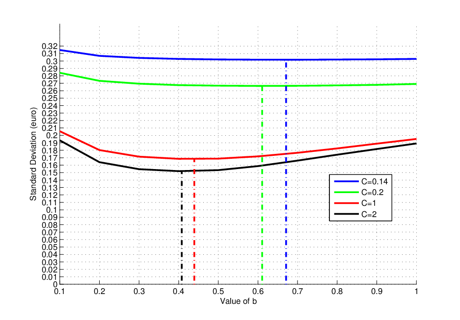
Moreover, we observe that the hedging error can be noticeably reduced by optimizing the rebalancing dates essentially for $C\geq 1$ i.e. around the Gaussian case. In these cases, one can observe on Figure 2 that the optimal rebalancing grid is noticeably different from the uniform grid since rebalancing dates are much more concentrated near maturity. This confirms the result of [21] that shows that, in the Gaussian case, taking a non uniform rebalancing grid (corresponding to $b=0.5$ ) allows to obtain a hedging error with the convergence order for the $L^{2}$ norm of $N^{-1/2}$ (up to a log factor) improving the rate $N^{-1/4}$ achieved with a uniform rebalancing grid (i.e. $b=1$ ), obtained in [26]. However, it is interesting to notice that this phenomenon is less pronounced when the tails of the log-returns distribution get heavier. In particular, one can observe on Figure 3 that the hedging error gets less sensitive to the rebalancing grid when $C$ decreases even if the optimal grid seems to get closer to the uniform grid.

	$C=2$	$C=1$	$C=0.2$	$C=0.14$
$10\times STD_{VO(\pi^{*})}$	$1.483$ $(30.82)$	$1.652$ $(34.33)$	$2.663$ $(54.80)$	$3.017$ $(61.53)$
$10\times STD_{VO(\pi^{b*})}$	$1.520$ $(31.58)$	$1.685$ $(35.01)$	$2.665$ $(54.84)$	$3.017$ $(61.53)$
$10\times STD_{VO(\pi^{1})}$	$1.892$ $(39.32)$	$1.952$ $(40.56)$	$2.691$ $(55.38)$	$3.028$ $(61.76)$
$V_{0}(\pi^{1})$	$0.4903$	$0.4859$	$0.4813$	$0.4812$
$V_{0}(\pi^{*})$	$0.4903$	$0.4860$	$0.4814$	$0.4813$
$b^{*}$	$0.4078$	$0.4394$	$0.6106$	$0.6710$

Table 2: Standard deviation of the Variance Optimal hedging error (

\times 10

) (reported within parenthesis in percent of the initial capital

V_{0}(\pi^{1})

), initial capitals for

b=1

and

b=b^{*}

, optimal grid parameters

b^{*}

, for different choices of parameters

C

with

N=12

and

K=99

(Digital option).

5.2 The case of electricity forward prices

We consider the problem of hedging and pricing a European call, with payoff $(F^{T_{d}}_{T}-K)_{+}$ , on an electricity forward, with a maturity $T=0.25$ of three month. The maturity $T$ is supposed to be equal to the delivery date of the forward contract $T=T_{d}$ . Because of non-storability of electricity, the hedging instrument is the corresponding forward contract. Then we set $S^{c}_{t}=F_{t}^{T}$ , where the forward price $F^{T}$ is supposed to follow the NIG one factor model (1.1) with $m\equiv 0,\sigma_{L}=0$ and $\sigma_{s}=\sigma>0$ . This gives

S^{c}_{t}=e^{X^{c}_{t}}\ ,\quad\textrm{where $X^{c}_{t}=\int_{0}^{t}\sigma e^{-\lambda(T-u)}d\Lambda_{u}$}\quad\textrm{where $\Lambda$ is a NIG process with }\quad\Lambda_{1}\,\sim\,{\rm NIG}(\alpha,\beta,\delta,\mu)\ .

(5.43)

Given $N+1$ discrete dates $0=t_{0}<t_{1}<\cdots<t_{N}=T$ , we consider the discrete process $X=X^{N}$ where $X_{k}=X^{c}_{t_{k}},0\leq k\leq N$ . We denote again by $z\mapsto m(z,k)$ the cumulant generating function associated with the increment $\Delta X_{k}=X_{k}-X_{k-1}$ for $k\in\{1,\cdots N\}$ . That function and its domain can be deduced from Lemma 3.24 and Proposition 6.2 in [28], see also (6.57). The domain $D$ contains $\tilde{D}:=[-\frac{\alpha+\beta}{\sigma},\frac{\alpha-\beta}{\sigma}]+i\mathbb{R}$ and given for any $z\in\tilde{D},k=0,\ldots,N,$

$\displaystyle m(z,k)$	$\displaystyle=$	$\displaystyle\mathbb{E}[\exp(z\int_{t_{k-1}}^{t_{k}}\sigma e^{-\lambda(T-u)}d\Lambda_{u})]$	(5.44)
	$\displaystyle=$	$\displaystyle\exp\left(\int_{t_{k-1}}^{t_{k}}\kappa^{\Lambda}(z_{u}du\right)\,,\quad\textrm{with }z_{u}=z\sigma e^{-\lambda(T-u)}$
	$\displaystyle=$	$\displaystyle\exp{\left(\int_{t_{k-1}}^{t_{k}}\big[\mu z_{u}+\delta\big(\sqrt{\alpha^{2}-\beta^{2}}-\sqrt{\alpha^{2}-(\beta+z_{u})^{2}}\big)\big]du\right)},$

where $\kappa^{\Lambda}$ is recalled in formula (6.57). Hence Assumption 2 1. is obviously satisfied since $\lambda\neq 0$ and Assumption 2 2. is verified as soon as $\sigma\leq\frac{\alpha-\beta}{2}$ ; thanks to Remark 3.15, Assumption 3 is automatically verified for the call representation given by Lemma 3.14.
Parameters are estimated on the same data as in the previous section, with Month-ahead base forward prices of the French Power market in 2007. For the distribution of $\Lambda_{1}$ this yields the following parameters

\alpha=15.81\,,\ \beta=-1.581\,,\ \delta=15.57\,,\ \mu=1.56\ ,

corresponding to a standard and centered NIG distribution with a skewness of $-0.019$ and excess kurtosis $0.013$ . The estimated annual short-term volatility and mean-reverting rate are $\sigma=57.47\%$ and $\lambda=3$ .

We have reported on Figure 4, the standard deviation of the hedging error as a function of the number of rebalancing dates for four types of hedging strategies.

•

Variance Optimal strategy (VO) with the uniform rebalancing grid (dark line) and with the optimal rebalancing grid $\pi^{\ast}$ (dark dashed line). Both variances are computed using formula (4.20) applied to the process (5.43);

•

Black-Scholes strategy (BS) implemented at the discrete instants of the uniform rebalancing grid (light line) and of the rebalancing grid $\pi^{\ast}$ (optimal for the Variance Optimal strategy) (light dashed line). Both variances are computed using Theorem 3.1 of [2] extended to non-stationary log-returns, to derive a quasi-explicit formula for the variance of the BS hedging error. Indeed, in [2], the authors uses the Laplace transform approach, to derive quasi-explicit formulae for the mean squared hedging error of various discrete time hedging strategies including Black-Scholes delta when applied to Lévy log-returns models. This extension of this result to the general case when $X$ is a non-stationary process with independent increments is given below.

Proposition 5.2.

Let $\upsilon$ be an admissible strategy satisfying

\upsilon_{n}=\int f^{\upsilon}(z)_{n}S^{z-1}_{n-1}\Pi(dz)

(5.45)

for $n=1,\dots,N$ , where $f^{\upsilon}(z)_{n}$ is a deterministic function of the complex variable $z$ . Let c be the initial capital; the bias and the variance of the hedging error $\epsilon(\upsilon,c):=H-c-\sum_{k=1}^{N}\upsilon_{k}\Delta S_{k}$ is given by

\mathbb{E}[\epsilon(\upsilon,c)]=\int S_{0}^{z}\left[\prod_{k=1}^{N}m(z,k)-\sum_{k=1}^{N}f^{\upsilon}(z)_{k}(m(1,k)-1)\prod_{l=2}^{k}m(z,l-1)\right]\Pi(dz)-c

(5.46)

\mathbb{E}[\epsilon(\upsilon,0)^{2}]=\int\int S_{0}^{y+z}(v_{1}(y,z)-v_{2}(y,z)-v_{3}(y,z)+v_{4}(y,z))\Pi(dz)\Pi(dy)\ ,

(5.47)

where

$\displaystyle v_{1}(y,z)$	$\displaystyle=$	$\displaystyle\prod_{k=1}^{N}m(y+z,k)$
$\displaystyle v_{2}(y,z)$	$\displaystyle=$	$\displaystyle\sum_{k=1}^{N}f^{\upsilon}(y)_{k}\,[m(z+1,k)-m(z,k)]\prod_{l=1}^{k-1}m(y+z,l)\prod_{l=k+1}^{N}m(z,l)$
$\displaystyle v_{3}(y,z)$	$\displaystyle=$	$\displaystyle\sum_{k=1}^{N}f^{\upsilon}(z)_{k}\,[m(y+1,k)-m(y,k)]\prod_{l=1}^{k-1}m(y+z,l)\prod_{l=k+1}^{N}m(y,l)$
$\displaystyle v_{4}(y,z)$	$\displaystyle=$	$\displaystyle\sum_{k=1}^{N}f^{\upsilon}(y)_{k}f^{\upsilon}(z)_{k}\,[m(2,k)-2m(1,k)+1]\prod_{l=1}^{k-1}m(y+z,l)$
		$\displaystyle+\sum_{j=2}^{N}\sum_{k<j}f^{\upsilon}(z)_{k}f^{\upsilon}(y)_{j}\,[m(y+1,k)-m(y,k)]\prod_{l=1}^{k-1}m(y+z,l)\prod_{l=k+1}^{j-1}m(y,l)(m(1,j)-1)$
		$\displaystyle+\sum_{j=2}^{N}\sum_{k>j}f^{\upsilon}(z)_{k}f^{\upsilon}(y)_{j}\,[m(z+1,j)-m(z,j)]\prod_{l=1}^{j-1}m(y+z,l)\prod_{l=j+1}^{k-1}m(z,l)(m(1,k)-1)\ .$

Therefore, the variance of the hedging error is

{\rm Var}(\epsilon(\upsilon;c))={\rm Var}(\epsilon(\upsilon;0))=\mathbb{E}[(\epsilon(\upsilon;0)^{2}]+\mathbb{E}[\epsilon(\upsilon;0)]^{2}\ .

Proof.

The proof is similar to the one of Theorem 3.1 of [2]. ∎

Remark 5.3.

In the case of Black-Scholes delta hedging strategy

f^{\upsilon}(z)_{n}=z\prod_{k=n}^{N}m^{bs}(z,k)\ ,\quad\textrm{where}\ m^{bs}(z,k)=\exp\left(-\frac{Var[\Delta X_{k}]}{2}z+\frac{Var[\Delta X_{k}]}{2}z^{2}\right).

Observing Figure 4, one can notice that, as expected, in all cases, the hedging error decreases when the number of trading dates increases. Observing the continuous lines, corresponding to a uniform rebalancing grid, one can notice the remarkable robustness of the Black-Scholes strategy. Indeed, in spite of the non Gaussianity of log-returns and the discreteness of the rebalancing grid, the Black-Scholes strategy is still quasi optimal in terms of variance.
Besides, in this case, the impact of the choice of the rebalancing grid seems to be more important than the choice of log-returns distribution (Gaussian or Normal Inverse Gaussian). For instance, using the VO strategy with the optimal rebalancing grid $\pi^{\ast}$ instead of $\pi^{1}$ allows to reduce $9\%$ (for $N=10$ ) of the hedging error standard deviation. The BS strategy shows similar performances to the VO case, when implemented at the rebalancing times $\pi^{\ast}$ . Indeed BS optimal rebalancing grid (in terms of variance) appears to be close to $\pi^{\ast}$ (up to $10^{-4}$ ). Moreover, one can observe on Table 3 that here again, the parametrization (5.42) of the rebalancing grid seems to be particularly well suited since it achieves minimal hedging errors comparable to the one achieved with the nonparametric optimal grid $\pi^{\ast}$ .

Notice that our analysis only considers the variance of the hedging error. To obtain the mean square error, one should add the bias contribution which is of course zero for the variance optimal strategy but it is in general non negligible for the Black-Scholes strategy. In particular, we can observe that this bias term varies strongly with the parameters of the NIG distribution.

For instance, for $N=2$ uniform rebalancing dates, replacing parameter $\beta$ by $-\beta$ increases the bias (defined as (5.46), with initial capital $c=V_{0}^{\rm BS})$ from -0.04 to 4.45. Moreover, one should also observe that the drift and the skewness of log-returns also impact the standard deviation of the BS hedging error. Changing again $\beta$ by $-\beta$ implies an increase of the log-returns expectation (resp. skewness) from 0 to 3.12 (resp. from -0.02 to 0.02) which induces an increase of the standard deviation of the BS hedging error from $4.91$ to $5.92$ , whereas the standard deviation of the VO hedging error decreases from 4.83 to 2.10.

	$N=2$	$N=5$	$N=10$	$N=25$	$N=50$
$STD_{VO(\pi^{*})}$	$4.5683$ $(53.23)$	$3.1129$ $(36.10)$	$2.3807$ $(27.56)$	$1.7790$ $(20.57)$	$1.5233$ $(17.61)$
$STD_{VO(\pi^{b*})}$	$4.57167$ $(53.27)$	$3.1550$ $(36.59)$	$2.4186$ $(28.00)$	$1.8023$ $(20.84)$	$1.5354$ $(17.75)$
$STD_{VO(\pi^{1})}$	$4.8331$ $(56.32)$	$3.4012$ $(39.44)$	$2.6154$ $(30.28)$	$1.9275$ $(22.29)$	$1.6145$ $(18.66)$
$STD_{BS(\pi^{1})}$	$4.9137$ $(57.26)$	$3.4196$ $(39.66)$	$2.6217$ $(30.35)$	$1.9329$ $(22.35)$	$1.6231$ $(18.76)$
$STD_{BS(\pi^{*})}$	$4.6291$ $(53.94)$	$3.1273$ $(36.27)$	$2.3884$ $(27.65)$	$1.7886$ $(20.68)$	$1.5344$ $(17.74)$
$V_{0}(\pi^{1})$	$8.5818$	$8.6232$	$8.6380$	$8.6469$	$8.6499$
$V_{0}(\pi^{*})$	$8.5895$	$8.6275$	$8.6406$	$8.6493$	$8.6531$
$b^{*}$	$0.5917$	$0.6298$	$0.6284$	$0.6203$	$0.6172$

Table 3: Standard deviation of the Variance Optimal hedging error (reported within parenthesis in percent of the initial capital

V_{0}(\pi^{1})

), initial capitals, optimal grid parameters

b^{*}

, for different choices of rebalancing dates

N

(Call option).

To analyze the impact of the rate of volatility increase on the optimal rebalancing grid, we have computed the hedging error standard deviation for several values of parameter $\lambda$ choosing the corresponding volatility parameter $\sigma$ such that $Var(X_{T})=\frac{\sigma^{2}}{2\lambda}(1-e^{-2\lambda T})$ is fixed. The resulting pairs $(\lambda,\sigma)$ are reported on Table 4. Coupling those parameters allows us to obtain comparable options for different parameters $\lambda$ ; at least this ensures a fixed initial capital in the BS framework (with $V_{0}^{BS}=8.7037$ ). On Figure 5, we have reported the optimal grid parameter $b^{\ast}$ minimizing the standard deviation of the VO hedging error for different values of $\lambda$ . As expected, when $\lambda$ increases, i.e. when the volatility increases more rapidly near the maturity, then $b^{\ast}$ decreases indicating that the optimal rebalancing dates concentrate near the maturity. On Figure 6, one can observe that the hedging error increases with $\lambda$ even when the rebalancing dates are optimized. However, optimizing the rebalancing dates allows to reduce noticeably the hedging error, specifically for high values of $\lambda$ . For instance, it allows to reduce $7.5\%$ of the error standard deviation when $\lambda=3$ and $17.9\%$ when $\lambda=9$ .

$\lambda$	$1$	$2$	$3$	$6$	$9$
$\sigma$	$0.4662$	$0.5202$	$0.5747$	$0.7349$	$0.8823$

Table 4: Short term volatility

\sigma

(s.t.

Var(X_{T})=\frac{\sigma^{2}}{2\lambda}(1-e^{-2\lambda T})

is fixed) for different values of parameter

\lambda

with

N=10

and

K=99

(Call option).

6 Appendix

A: A general convergence theorem for FS decompositions

Proposition 6.1.

Let $(H^{\ell})_{\ell\in\mathbb{N}\cup\{+\infty\}}$ be a sequence of r.v. in ${\cal L}^{2}(\Omega,{\cal F}_{N})$ . Let

\left\{\begin{array}[]{ccc}H_{n}^{\ell}&=&H_{0}^{\ell}+\sum_{i=1}^{n}\xi^{\ell}_{i}\Delta S_{i}+L_{n}^{\ell}\\ H_{N}^{\ell}&=&H^{\ell}\end{array}\right.

(6.48)

be the FS-decomposition of $H^{\ell}$ . Suppose that $H^{\ell}\rightarrow H^{\infty}$ in ${\cal L}^{2}(\Omega)$ . Then, for $\ell\rightarrow+\infty$ ,

1.

$H_{0}^{\ell}\rightarrow H_{0}^{\infty}$ in ${\cal L}^{2}({\cal F}_{0})$ ;
2.

$\xi_{n}^{\ell}\rightarrow\xi_{n}^{\infty}$ in probability for any $n\in\{1,\dots,N\}$ ;
3.

$L_{N}^{\ell}\rightarrow L_{N}^{\infty}$ in ${\cal L}^{2}(\Omega)$ .

Proof.

For $n\in\{1,\dots,N\}$ , $\ell\in\mathbb{N}\cup\{+\infty\}$ we have

H_{n}^{\ell}=H^{\ell}_{n-1}+\xi^{\ell}_{n}\Delta S_{n}+\Delta L^{\ell}_{n}.

(6.49)

For technical reasons we set $\xi^{\ell}_{N+1}:=0$ and $L^{\ell}_{N+1}:=L^{\ell}_{N}$ . The result will follow if for every $n\in\{0,\dots,N\}$ , for $\ell\rightarrow+\infty$ we have

1.

$H_{n}^{\ell}\rightarrow H_{n}^{\infty}$ in ${\cal L}^{2}$ ,
2.

$\mathbb{E}\left[\left(\Delta S_{n+1}\right)^{2}\left(\xi^{\ell}_{n+1}-\xi^{\infty}_{n+1}\right)^{2}\right]\rightarrow 0$ ,
3.

$L^{\ell}_{n+1}\rightarrow L^{\infty}_{n+1}$ in ${\cal L}^{2}$ .

We will prove 1.,2. and 3. by backward induction on $n\in\{0,\dots,N\}$ starting from $n=N$ . The step $N$ of the induction is constituted by the assumption, in particular 1. and 3. are verified by assumption and 2. is trivially verified.
Suppose that 1.,2. and 3. hold for some $n\in\{1,\dots,N\}$ , we will prove their validity for the integer $n-1$ . First, 1. implies that $\mathbb{E}\left[H_{n}^{\ell}|{\cal F}_{n-1}\right]\rightarrow_{\ell\rightarrow+\infty}\mathbb{E}\left[H_{n}^{\infty}|{\cal F}_{n-1}\right]$ in ${\cal L}^{2}(\Omega)$ . We continue taking the conditional expectation with respect to ${\cal F}_{n-1}$ in (6.49). This gives

\mathbb{E}\left[H_{n}^{\ell}|{\cal F}_{n-1}\right]=H^{\ell}_{n-1}+\xi^{\ell}_{n}\Delta A_{n}.

(6.50)

The difference between (6.49) and (6.50) gives

H_{n}^{\ell}-\mathbb{E}\left[H_{n}^{\ell}|{\cal F}_{n-1}\right]=\xi^{\ell}_{n}\Delta M_{n}+\Delta L_{n}^{\ell},\ \ell\in\mathbb{N}\cup\{+\infty\}.

Consequently

H_{n}^{\ell}-H_{n}^{\infty}=\mathbb{E}\left[H_{n}^{\ell}-H_{n}^{\infty}|{\cal F}_{n-1}\right]=\left(\xi^{\ell}_{n}-\xi^{\infty}_{n}\right)\Delta M_{n}+\Delta(L_{n}^{\ell}-L_{n}^{\infty}).

\mathbb{E}\left[\left(H_{n}^{\ell}-H_{n}^{\infty}\right)-\mathbb{E}\left[H_{n}^{\ell}-H_{n}^{\infty}|{\cal F}_{n-1}\right]^{2}\right]=\mathbb{E}\left[\left(\xi^{\ell}_{n}-\xi^{\infty}_{n}\right)^{2}\left(\Delta M_{n}\right)^{2}\right]+\mathbb{E}\left[\Delta\left(L_{n}^{\ell}-L_{n}^{\infty}\right)\right]^{2};

(6.51)

in fact

\mathbb{E}\left(\left(\xi^{\ell}_{n}-\xi^{\infty}_{n}\right)\Delta M_{n}\Delta\left(L_{n}^{\ell}-L_{n}^{\infty}\right)\right)=\mathbb{E}\left((\xi^{\ell}_{n}-\xi^{\infty}_{n})\mathbb{E}\left((\Delta M_{n})\Delta(L_{n}^{\ell}-L_{n}^{\infty})|{\cal F}_{n-1}\right)\right)=0,

because $M.\left(L^{\ell}-L^{\infty}\right)$ is a martingale. Since the left-hand side of (6.51) converges to zero when $\ell\rightarrow\infty$ , it follows that

	$\displaystyle\mathbb{E}\left[\left(\xi^{\ell}_{n}-\xi^{\infty}_{n}\right)^{2}\left(\Delta M_{n}\right)^{2}\right]$	$\displaystyle\rightarrow_{\ell\rightarrow\infty}$	$\displaystyle 0$		(6.52)
	$\displaystyle\mathbb{E}\left[\Delta\left(L_{n}^{\ell}-L_{n}^{\infty}\right)\right]^{2}$	$\displaystyle\rightarrow_{\ell\rightarrow\infty}$	$\displaystyle 0.$

This shows 2. and 3. of the $(n-1)$ -step of the backward induction. It remains to show item 1. By (6.49), we have

H_{n-1}^{\ell}-H_{n-1}^{\infty}=H_{n}^{\ell}-H_{n}^{\infty}-\Delta S_{n}\left(\xi^{\ell}_{n}-\xi^{\infty}_{n}\right)-\Delta\left(L_{n}^{\ell}-L_{n}^{\infty}\right).

Since $H_{n}^{\ell}-H_{n}^{\infty}$ and $\Delta\left(L_{n}^{\ell}-L_{n}^{\infty}\right)$ converge to zero in ${\cal L}^{2}$ , it remains to show that $\Delta S_{n}\left(\xi^{\ell}_{n}-\xi^{\infty}_{n}\right)\rightarrow_{\ell\rightarrow\infty}0$ in ${\cal L}^{2}(\Omega)$ when $\ell\rightarrow\infty$ . Now $\Delta M_{n}\left(\xi^{\ell}_{n}-\xi^{\infty}_{n}\right)\rightarrow_{\ell\rightarrow\infty}0$ in ${\cal L}^{2}(\Omega)$ and so by (6.52) we only have to prove that

\mathbb{E}\left[\left(\xi^{\ell}_{n}-\xi^{\infty}_{n}\right)^{2}\left(\Delta A_{n}\right)^{2}\right]\rightarrow_{\ell\rightarrow\infty}0.

(6.53)

By the (ND) condition and item 1. of Remark 2.4, we have

	$\displaystyle\left(\Delta A_{n}\right)^{2}$	$\displaystyle=$	$\displaystyle\left(\mathbb{E}\left(\Delta S_{n}\|{\cal F}_{n-1}\right)\right)^{2}\leq\delta\mathbb{E}\left(\left(\Delta S_{n}\right)^{2}\|{\cal F}_{n-1}\right)$
		$\displaystyle=$	$\displaystyle\delta\left((\Delta A_{n})^{2}+\mathbb{E}\left[\left(\Delta M_{n}\right)^{2}\|{\cal F}_{n-1}\right]\right).$

Consequently

\displaystyle\left(\Delta A_{n}\right)^{2}

\displaystyle\leq

\displaystyle\frac{\delta}{1-\delta}\mathbb{E}\left[\left(\Delta M_{n}\right)^{2}|{\cal F}_{n-1}\right].

So the left-hand side of (6.53) is bounded by

\frac{\delta}{1-\delta}\mathbb{E}\left[\left(\xi^{\ell}_{n}-\xi_{n}^{\infty}\right)^{2}\left(\Delta M_{n}\right)^{2}\right]\rightarrow_{\ell\rightarrow\infty}0.

The result is finally established. ∎

B: The Normal Inverse Gaussian distribution

The Normal Inverse Gaussian (NIG) distribution is a specific subclass of the Generalized Hyperbolic family introduced by Barndorff–Nielsen in 1977, see for instance [3]. The density of a Normal Inverse Gaussian distribution of parameters $(\alpha,\beta,\delta,\mu)$ is given by

f_{NIG}(x;\alpha,\beta,\delta,\mu)=\frac{\alpha}{\pi}\exp\big(\delta\sqrt{\alpha^{2}-\beta^{2}}+\beta(x-\mu)\big)\frac{K_{1}\big(\alpha\delta\sqrt{1+(x-\mu)^{2}/\delta^{2}}\big)}{\sqrt{1+(x-\mu)^{2}/\delta^{2}}}\ ,\quad\textrm{for any}\ x\in\mathbb{R}\ ,

(6.54)

where $K_{1}$ denotes the Bessel function of the third type with index $1$ and where the parameters are such that $\delta>0$ , $\alpha>0$ and $\alpha>|\beta|$ . Afterwards, NIG $(\alpha,\beta,\delta,\mu)$ will denote the Normal Inverse Gaussian distribution of parameters $(\alpha,\beta,\delta,\mu)$ .

A useful property of the NIG distribution is its stability under convolution i.e.

NIG(\alpha,\beta,\delta_{1},\mu_{1})\ast NIG(\alpha,\beta,\delta_{2},\mu_{2})=NIG(\alpha,\beta,\delta_{1}+\delta_{2},\mu_{1}+\mu_{2})\ .

This property shared with the Gaussian distribution allows to simplifies many computations.

If $X$ is a NIG( $\alpha,\beta,\delta,\mu$ ) random variable then for any $a\in\mathbb{R}^{+}$ and $b\in\mathbb{R}\,,$ $Y=aX+b$ is also a NIG random variable with parameters ( $\alpha/a,\beta/a,a\delta,a\mu+b$ ).

The mean and the variance associated to a NIG $(\alpha,\beta,\delta,\mu)$ random variable $X$ are given by,

\mathbb{E}X=\mu+\frac{\delta\beta}{\gamma}\ ,\quad\textrm{Var}X=\frac{\delta\alpha^{2}}{\gamma^{3}}\ ,\quad\textrm{with}\quad\gamma=\sqrt{\alpha^{2}-\beta^{2}}\ .

(6.55)

The characteristic function of the NIG distribution is given by $\exp(\Psi_{NIG})$ where $\Psi_{NIG}$ verifies

\Psi_{NIG}(u)=\log\mathbb{E}\big[\exp(iuX)\big]=i\mu u+\delta(\sqrt{\alpha^{2}-\beta^{2}}-\sqrt{\alpha^{2}-(\beta+iu)^{2}})\quad\textrm{for any}\quad u\in\mathbb{R}\ .

(6.56)

The moment generating function of the NIG distribution is particularly simple,

\kappa^{\Lambda}(z)=\kappa^{\Lambda}_{NIG}(z)=\log\mathbb{E}[\exp(zX)]=\mu z+\delta\big(\sqrt{\alpha^{2}-\beta^{2}}-\sqrt{\alpha^{2}-(\beta+z)^{2}}\big)\ ,\quad\textrm{for}\ Re(z)\in[-(\alpha+\beta);\alpha-\beta]\ .

(6.57)

The Lévy measure of the NIG distribution is given by

F_{NIG}(dx)=e^{\beta x}\frac{\delta\alpha}{\pi|x|}K_{1}(\alpha|x|)\,dx\quad\textrm{for any}\ x\in\mathbb{R}\ .

(6.58)

Notice that the Lévy measure does not depend on parameter $\mu$ .

ACKNOWLEDGEMENTS: The authors are grateful to the anonymous Referee for her $\backslash$ his stimulating remarks and comments which allowed them to considerably improve the first version of the paper.

The first named author was partially founded by Banca Intesa San Paolo. The research of the third named author was partially supported by the ANR Project MASTERIE 2010 BLAN-0121-01.

References

[1] Angelini, F. and Herzel., S. (2010). Explicit formulas for the minimal hedging strategy in a martingale case. Decisions in Economics and Finance Vol 33(1).
[2] Angelini, F. and Herzel., S. (2009). Measuring the error of dynamic hedging: a Laplace transform approach. Computational Finance Vol 12(2).
[3] Barndorff-Nielsen, O.E. and Halgreen, C. (1977). Infinite divisibility of the hyperbolic and generalized inverse Gaussian distributions Zeitschrift für Wahrscheinlichkeitstheorie und verwandte Gebiete, Vol. 38, 309-312.
[4] Barndorff-Nielsen, O.E. (1998). Processes of normal inverse Gaussian type, Finance and Stochastics 2, 41-68.
[5] Benth, F. E., Kallsen, J. and Meyer-Brandis, T. (2007). A non-Gaussian Ornstein-Uhlenbeck process for electricity spot price modeling and derivatives pricing, Applied Mathematical Finance, 14(2), 153-169.
[6] Benth, F. E., Di Nunno, G., Løkka, A., Øksendal, B. and Proske, F. (2003). Explicit representation of the minimal variance portfolio in markets driven by Lévy processes. Conference on Applications of Malliavin Calculus in Finance (Rocquencourt, 2001). Mathematical Finance 13, no. 1, 55–72.
[7] Benth, F.E. and Saltyte-Benth, J. (2004). The normal inverse Gaussian distribution and spot price modeling in energy markets, International journal of theoretical and applied finance, Vol. 7(2), 177-192.
[8] Bertsimas, D., Kogan, L. and Lo, A. W. (2001). Hedging derivative securities and incomplete markets: an $\epsilon$ -arbitrage approach, Oper. Res. 49, no. 3.
[9] $\check{C}$ ern $\grave{y}$ A. (2004). Dynamic Programming and Mean-Variance Hedging in Discrete Time, Applied Mathematical Finance 11(1), 1-25.
[10] $\check{C}$ ern $\grave{y}$ A. (2007). Optimal Continuous-Time Hedging with Leptokurtic Returns, Mathematical Finance, Vol. 17(2), pp. 175-203.
[11] $\check{C}$ ern $\grave{y}$ , A. and Kallsen, J. (2007). On the structure of general man-variance hedging strategies, The Annals of probability, Vol. 35 N. 4, 1479-1531.
[12] $\check{C}$ ern $\grave{y}$ , A. and Kallsen, J. (2009). Hedging by sequential regressions revisited. Math. Finance 19, no. 4, 591–617.
[13] Collet, J., Duwig D. and Oudjane N. (2006). Some non-Gaussian models for electricity spot prices, In Proceedings of the 9th International Conference on Probabilistic Methods Applied to Power Systems 2006.
[14] Cont, R. and Tankov, P. (2003). Financial modeling with Jump Processes Chapman & Hall / CRC Press.
[15] Cont, R., Tankov, P. and Voltchkova, E. (2007). Hedging with options in models with jumps. Stochastic analysis and applications, 197–217, Abel Symp., 2, Springer, Berlin.
[16] Cox, J. C., Ross, S. A. and Rubinstein, M. (1979). Option Pricing: A Simplified Approach. Journal of Financial Economics 7: 229-263.
[17] Denkl, S., Goy, M., Kallsen, J., Muhle-Karbe, J. and Pauwels, A. (2009). On the performance of delta-hedging strategies in exponential Lévy models. Preprint.
[18] Duffie, D. and Richardson H.R. (1991). Mean-variance hedging in continuous time. Ann. Appl. Probab. 1, no. 1, 1–15.
[19] Föllmer, H. and Schweizer, M. (1989). Hedging by Sequential Regression: An Introduction to the Mathematics of Option Trading. The ASTIN Bulletin 18, 147–160.
[20] Föllmer, H. and Schweizer, M. (1991). Hedging of contingent claims under incomplete information. Applied stochastic analysis (London, 1989), 389-414, Stochastics Monogr., 5, Gordon and Breach, New York.
[21] Geiss, S. (2002). Quantitative approximation of certain stochastic integrals. Stoch. Stoch. Rep., 73(3-4):241-270.
[22] Geiss, C. and Geiss, S. (2004). On approximation of a class of stochastic integrals and interpolation. Stoch. Stoch. Rep. 76, no. 4, 339–362.
[23] Geiss S. and Gobet E. (2011). Fractional smoothness and applications in finance. Preprint arXiv:1004.3577v1. To appear in AMAMEF book, G. Di Nunno and B. Øksendal Eds.
[24] Gobet, E. and Makhlouf, A. (2010). The tracking error rate of the Delta-Gamma hedging strategy. To appear: Mathematical finance. Available at http://hal.archives-ouvertes.fr/hal-00401182/fr/.
[25] Gourieroux, C., Laurent, J.-P. and Pham, H. (1998). Mean-variance hedging and numéraire. Math. Finance 8, no. 3, 179–200.
[26] Gobet, E. and Temam, E. (2001). Discrete time hedging errors for options with irregular pay-offs. Finance and Stochastics 5(3):357–367.
[27] Goll, T. and Ruschendorf, L. (2002). Minimal distance martingale measures and optimal portfolios consistent with observed market process, Stochastic Processes and Related Topics, 8 141-154.
[28] Goutte, S., Oudjane, N. and Russo, F. (2009). Variance Optimal Hedging for continuous time processes with independent increments and applications. Preprint HAL inria-00437984, http://fr.arxiv.org/abs/0912.0372.
[29] Hubalek, F., Kallsen, J. and Krawczyk, L.(2006). Variance-optimal hedging for processes with stationary independent increments, The Annals of Applied Probability, Vol. 16, Number 2, 853-885.
[30] Kallsen, J. and Pauwels, A. (2011). Variance-optimal hedging for time-changed Lévy processes, Appl. Math. Finance 18, no. 1, 1-28.
[31] Kallsen, J. and Pauwels, A. (2010). Variance-optimal hedging in general affine stochastic volatility models, Advances in Applied Probability 20 no. 1, 83-105.
[32] Kallsen, J., Muhle-Karbe, J., Shenkman, N. and Vierthauer, R. (2009). Discrete-time variance-optimal hedging in affine stochastic volatility models. In R. Kiesel, M. Scherer, and R. Zagst, editors, Alternative Investments and Strategies. World Scientific, Singapore.
[33] Rheinländer, T. and Schweizer, M. (1997). On $L^{2}$ -projections on a space of stochastic integrals, Ann. Probab. 25, no. 4, 1810–1831.
[34] Rudin, W. (1987). Real and complex analysis, third edition. New York: McGraw-Hill.
[35] Schäl, M. (1994). On quadratic cost criteria for options hedging, Mathematics of Operations Research 19, 121-131.
[36] Schweizer, M. (1994). Approximating random variables by stochastic integrals, The Annals of Probability Vol. 22, 1536-1575.
[37] Schweizer, M. (1995). On the minimal martingale measure and the Föllmer-Schweizer decomposition, Stochastic Analysis and Applications, 13, no. 5, 573–599.
[38] Schweizer, M. (1995). Variance-optimal hedging in discrete time, Mathematics of Operations Research 20, 1-32.
[39] Schweizer, M. (2001). A guided tour through quadratic hedging approaches. Option pricing, interest rates and risk management, 538-574, Handb. Math. Finance, Cambridge Univ. Press, Cambridge.

Variance Optimal Hedging for discrete time processes with independent increments. Application to Electricity Markets

Abstract

1 Introduction

2 Generalities and Discrete Föllmer-Schweizer decomposition

Definition 2.1.

Definition 2.2.

Remark 2.3.

Remark 2.4.

Remark 2.5.

Definition 2.6.

Proposition 2.7.

Proof.

Definition 2.8.

2.1 Existence and structure of an optimal strategy

Assumption 1.

Remark 2.9.

Proposition 2.10.

Proof.

Theorem 2.11.

Proof.

3 Exponential of PII processes

Definition 3.1.

3.1 Discrete cumulant generating function

Definition 3.2.

Remark 3.3.

Remark 3.4.

Assumption 2.

Remark 3.5.

Lemma 3.6.

Proof.

Lemma 3.7.

Proof.

Remark 3.8.

Remark 3.9.

Proposition 3.10.

Proof.

3.2 Discrete Föllmer-Schweizer decomposition

Proposition 3.11.

Remark 3.12.

Remark 3.13.

Proof of Proposition 3.11.

3.3 Discrete Föllmer-Schweizer decomposition of special contingent claims

Lemma 3.14.

Assumption 3.

Remark 3.15.

Remark 3.16.

Remark 3.17.

Lemma 3.18.

Proof.

Proposition 3.19.

Proof.

4 The solution of the minimization problem

4.1 Mean-Variance Hedging

Theorem 4.1.

Remark 4.2.

Proof of theorem 4.1.

4.2 The Hedging Error

Theorem 4.3.

Remark 4.4.

Proof.

Proposition 4.5.

Proof.

Proposition 4.6.

Proof.

5 Numerical results

5.1 The case of a Digital option

Proposition 5.1.

Proof.

5.2 The case of electricity forward prices

Proposition 5.2.

Proof.

Remark 5.3.

6 Appendix

A: A general convergence theorem for FS decompositions

Proposition 6.1.

Proof.

B: The Normal Inverse Gaussian distribution

References

Variance Optimal Hedging for discrete time processes with independent increments.
Application to Electricity Markets