Angular momentum transport and variability in boundary layers of accretion disks driven by global acoustic modes.
Abstract
Disk accretion onto a weakly magnetized central object, e.g. a star, is inevitably accompanied by the formation of a boundary layer near the surface, in which matter slows down from the highly supersonic orbital velocity of the disk to the rotational velocity of the star. We perform high resolution 2D hydrodynamical simulations in the equatorial plane of an astrophysical boundary layer with the goal of exploring the dynamics of non-axisymmetric structures that form there. We generically find that the supersonic shear in the boundary layer excites non-axisymmetric quasi-stationary acoustic modes that are trapped between the surface of the star and a Lindblad resonance in the disk. These modes rotate in a prograde fashion, are stable for hundreds of orbital periods, and have a pattern speed that is less than and of order the rotational velocity at the inner edge of the disk. The origin of these intrinsically global modes is intimately related to the operation of a corotation amplifier in the system. Dissipation of acoustic modes in weak shocks provides a universal mechanism for angular momentum and mass transport even in purely hydrodynamic (i.e. non-magnetized) boundary layers. We discuss the possible implications of these trapped modes for explaining the variability seen in accreting compact objects.
Keywords:
accretion, accretion disks – hydrodynamics — waves – instabilitiesI Introduction
One of the outstanding problems in astrophysical accretion disk theory is the physics of the boundary layer (hereafter BL). The BL is the innermost region of the accretion disk in which the rotation profile of the star attaches smoothly to that of the disk [27]. In the BL, the rotation velocity of the disk fluid necessarily rises with increasing radius, which has important implications for angular momentum transport. BLs occur in a variety of systems — young stars, white dwarfs, neutron stars — whenever the accretion rate is high enough for the disk to extend all the way down to the surface of the central object (hereafter referred to as “star” for simplicity), without being disrupted by the stellar magnetic field. In such cases, up to half of the accretion energy is dissipated in the BL [22], which leads to intense local heating and gives rise to X-ray and ultraviolet emission in accreting neutron stars [18] and white dwarfs [40, 41, 30, 38, 36].
Since the rotational velocity of the gas passing through the BL changes with radius, some mechanism of angular momentum transport must operate there, ultimately leading to the radial mass transport. The nature of this mechanism is not understood at the moment. The magnetorotational instability (MRI; Velikhov [51], Chandrasekhar [11], Balbus & Hawley [4], Balbus & Hawley [5]) usually invoked to explain mass transport in accretion disks does not operate in the BL because there ( is the cylindrical radius). Magnetic field carried into the BL by accreting gas is sheared by differential rotation [1, 47] but whether this can lead to sustained mass accretion has not been conclusively demonstrated. Other transport mechanisms — Kelvin-Helmholtz instability [20], baroclinic instability [12], Tayler-Spruit dynamo [49, 46, 36] have also been proposed but whether they can operate in the BL and give rise to efficient momentum transport there is far from clear. In the absence of a good understanding of the momentum and mass transport, even the morphology of the BL has been a matter of debate, with the proposed geometries ranging from a BL contained inside the star[20] to a spreading layer extending to significant latitudes over the stellar surface [18, 19].
The BL has also been associated with variability in accreting systems that occurs on timescales comparable to the dynamical timescale at the surface of the star. One example of such variability are dwarf nova oscillations (DNOs) in accreting white dwarf systems [52], which do not have a definitive explanation. DNOs are characterized by an oscillation period of , where is the DNO period and is the Keplerian rotational period at the surface of the star [35]. Since the DNO period is comparable to the Keplerian rotational period at the surface of the star, it is natural to associate DNOs with the boundary layer or with the region of the disk directly adjacent to it.
In this work we describe a set of first principles, two-dimensional (2D) hydrodynamical simulations of the equatorial plane of the disk-star system carried out in cylindrical geometry. The main result of our work is that we generically observe the excitation of a non-axisymmetric mode in the BL with a unique wavelength and pattern speed that is stable for many hundreds of orbital periods.
The mechanism of excitation for this mode is the sonic instability [13, 8], which is a type of shear instability that occurs for supersonic, highly compressible flows. The sonic instability is closely related to the Papaloizou-Pringle instability [34, 31] and operates very differently from the more familiar KH instability, which occurs in the subsonic regime.
Dissipation of the non-axisymmetric BL mode by virtue of weak shocks results in angular momentum and mass transport in the BL. It has also been argued that the presence of a non-axisymmetric mode in the BL or on the surface of the star can modulate stellar emission, providing an explanation for DNOs [33, 39, 37]. Previously, however, there was no acknowledged mechanism for exciting non-axisymmetric modes on the surface of the star. Since such modes emerge naturally in our simulations, our work may help to understand the mechanism of DNOs, or more generically, any periodic phenomena having a period .
The paper is organized as follows: In §II we present the model we use in our simulations, and in §III we present our results. We find that the boundary layer is unstable to sonic instabilities (§III.1), which tend to excite a single surface mode. This mode is characterized by vortices at the base of the BL and by shocks launched from the top of the BL that propagate through the disk and are reflected back towards the BL at a Lindblad resonance. The shocks are weak with a small compression ratio, and we find that their properties can be easily understood in terms of the WKB theory for weak disturbances in the disk (§III.2). We also study the stresses in the BL caused by the instabilities that operate there (§III.3-III.5), transport of mass (§III.6+), how the pattern speed of the modes is affected by Mach number (§III.7), and how the BL thickness varies as a function of both time and Mach number (§III.8). In §IV, we simulate the full range of azimuthal angle from and observe long wavelength non-axisymmetric modes.
II Numerical Model
We perform a set of 2D hydrodynamical simulations in the equatorial () plane of a star with an adjacent accretion disk. This setup ignores the vertical structure of the disk and star but allows us to capture the formation of the long-lived, non-axisymmetric structures in the BL at reasonable numerical cost. Similar to Armitage [1] and Steinacker & Papaloizou [47] we disregard thermodynamical evolution of the system by adopting the isothermal equation of state in our simulations, so the pressure is given by
| (1) |
Here is the density, and is the isothermal sound speed, which we assume to be the same throughout the simulation domain. Adoption of isothermal equation of state is equivalent to assuming fast cooling in the BL. This may not be realistic for all systems, but we still adopt this approximation since we are primarily interested in providing a proof of concept for the trapped acoustic modes, which are the main focus of our paper.
Previously, Armitage [1], Steinacker & Papaloizou [47], Romanova et al. [43] have performed 3D MHD simulations of the BL. We plan to include magnetic fields in future 3D simulations, but first it is useful to investigate and understand the restricted 2D hydro case, since it allows us to study in detail trapped modes excited by sonic instabilities, which are the main focus of our paper.
We numerically evolve the following set of equations
| (2) | |||
| (3) |
in the equatorial plane of the disk+star system, where is a fixed, time-independent potential. The system of equations is closed by the isothermal equation of state, equation (1).
For the numerical evolution of equations (2) and (3), we use the Godunov code Athena [48] in cylindrical coordinates [45]. Athena is highly-parallelized and exhibits very low levels of numerical viscosity (§III.6) making it well-suited for studying the long-term evolution of the boundary layer.
We use a significantly higher resolution than previous authors, which lets us properly resolve the scale height of the star. This is important for studying modes excited in the BL, since the scale height represents a natural length scale in the problem. Balsara et al. [7] have also run high resolution 2D simulations of the BL in the meridional () plane, but the axisymmetric setup of their simulations precluded them from seeing the sonic instability. Moreover, their simulations were run for orbital period, whereas we run our simulations for hundreds of orbital periods, as measured at the inner radius of the disk. This allows us to investigate the long-term evolution of the BL and observe the stability of modes excited on the star on very long timescales.
II.1 Physical Setup
In our initial setup, we consider a non-rotating star in hydrostatic equilibrium which is surrounded by a rotationally supported disk of constant density. We nondimensionalize quantities by setting the radius of the star to , the Keplerian orbital velocity at the surface of the star to , and the surface density in the disk to . Thus, time is scaled such that the Keplerian orbital period is at , where is the cylindrical radius. We take the potential in the system to be given by the fixed cylindrically-symmetric potential
| (4) |
and we ignore self-gravity in the simulations. Since the potential given by Equation 4 is cylindrically symmetric, our calculations do not include the vertical stratification of the disk.
At the start of the simulation, the star is joined to the disk via a thin region of width , inside of which the rotational velocity rises very nearly linearly from zero (the velocity in the star) to the Keplerian orbital velocity (the velocity in the disk). The initial rotation profile is given by
and from now on, when speaking about the initial conditions of the simulations, we will refer to the region as the “star”, the region as the “interface”, and the region as the “disk”, see Figure 1. It is important to bear in mind, though, that the rotation profile will evolve in time as a result of sonic instabilities (discussed below) that induce angular momentum transport. These instabilities will rapidly cause the initial “interface” region to thicken into a self-consistent BL, see §III.1.
The initial density profile is specified everywhere throughout the domain through the equation of hydrostatic equilibrium
| (9) |
This results in within the disk, and within the star. Figure 1 shows the initial rotation profile from equation (II.1), as well as the initial density profile which is determined by hydrostatic equilibrium.
For each of our simulations we define a characteristic Mach number , where is the isothermal sound speed. In our units the gravitational acceleration is at (equation 4), which means that corresponds to the actual Mach number at for a Keplerian disk, since the Keplerian velocity is at in our simulations. We also define a characteristic radial scale in the star using
| (10) |
This is the exact pressure and density scale height at for an unrotating flow since
| (11) |
and can be written in terms of the Keplerian velocity as . Plugging this into equation (11) and using , we recover equation (10). Note that is different from the scale height of the accretion disk in the vertical direction (which is not considered in our simulations). The latter is given by so that .
At this point it is clear that if the isothermal equation of state is assumed, the only free parameter in the problem is the Mach number. However, we emphasize this point by explicitly showing that this is the case. To do so, we non-dimensionalize the isothermal fluid dynamics equations by scaling the unit of length according to , the unit of time according to , and the density according to , which is some arbitrary density, such as the density of the disk which is a constant in our model. Assuming a Keplerian rotation profile ( form of the potential), equations (2) and (3) become
| (12) | |||
| (13) |
where , and the primes denote the non-dimensionalized forms of the variables and operators, i.e. , , etc. When the equations are written in non-dimensionalized form, it is clear that the Mach number is the only free parameter in the problem for a fixed geometry. Thus, the solutions for the isothermal boundary layer form a one-parameter family in the Mach number, and the Mach number itself plays a role which is analogous to the Reynolds number for the incompressible Navier-Stokes equations. Of course, if the isothermal assumption is relaxed, the solution will also depend on other dimensionless parameters. However, since this paper is a proof of concept, we do not concern ourselves with those parameters here.
II.2 Numerical Details
We now summarize the numerical details which pertain to all of our simulations, and we begin by discussing the condition of hydrostatic equilibrium. Zingale et al. [55] discuss how to set the initial conditions to achieve numerical hydrostatic equilibrium in a Godunov code. However, we opt for a simpler approach in which we initialize the simulation according to a numerical integration of equation (9) and wait for the fluctuations from the initial transient to damp out.
The amplitude of the initial fluctuations depends on the resolution of the simulation, but even small fluctuations close to the inner radial boundary can amplify to become shocks as they propagate into the disk. This is due to the fact that the amplitude of a wave propagating in an isothermal atmosphere is [23] and there is a large density contrast between the density in the disk and the density at the inner radius of the simulation domain (factor of ). For this reason, we burn in all of our simulations by running the analytic hydrostatic equilibrium solution for a time of with no perturbations, which allows the simulation to settle down to a numerical hydrostatic equilibrium.
| label | -range | -range | ||
|---|---|---|---|---|
| A1 | (0.7, 2.5) | (-0.4, 0.4) | 6 | |
| A2 | (0.7, 2.5) | (-0.4, 0.4) | 6 | |
| A3 | (0.7, 2.5) | (-0.4, 0.4) | 6 | |
| A4 | (0.7, 2.5) | (0, 2) | 6 | |
| A5 | (0.7, 4.3) | (-0.4, 0.4) | 6 | |
| B1 | (0.85, 2.5) | (-0.4, 0.4) | 9 | |
| B2 | (0.85, 2.5) | (0, 2) | 9 | |
| C1 | (0.9, 2.5) | (-0.4, 0.4) | 12 | |
| C2 | (0.9, 2.5) | (0, 2) | 12 | |
| D1 | (0.94, 2.5) | (-0.4, 0.4) | 15 | |
| D2 | (0.94, 2.5) | (0, 2) | 15 |
We then restart the simulation by adding a random perturbation to the radial velocity, , at each grid point for , and for the remainder of the paper we take to be the time when the perturbations are added. The reason not to create perturbations to the velocity within the star stems from the fact that the density rises exponentially inside the star, and any disturbance propagating from the star towards the disk amplifies exponentially as well, with the relative amplitude going as the inverse square root of the density [23].
The boundary conditions we use for the simulations are periodic in and “do-nothing” at the inner and outer radial boundaries. The do-nothing boundary condition simply means that the fluid variables on the boundary retain their initial values for the duration of the simulation. This is a convenient boundary condition to use, since essentially no action takes place near the inner or outer boundaries: there is no mass inflow or outflow through these boundaries, and any incident waves are largely absorbed with minimal reflection.
In order to accurately capture the physics of modes excited on the surface of the star (§III.2), it is both necessary that the simulation extend to several stellar radii, and that we resolve the radial scale height (equation [10]) inside the star. To satisfy the second of these conditions, we use cells per radial scale height within the star, depending on the simulation. However, the first condition that the simulation domain extend to several stellar radii makes it computationally prohibitive to run the simulations at realistic Mach numbers, since the scale height goes as . As a compromise, we use for our simulations, even though this is somewhat low in an astrophysical context. For example, a typical accreting white dwarf has an inner disk temperature of , a stellar radius of , and a mass of , meaning that
| (14) |
for such a system.
In all of our simulations we use for the width of the interface, so that . This is as thin as we can make the interface region, while still being able to resolve the physics that goes on there.
Table 1 summarizes the parameters of our simulations. In all of our simulations, we only vary one physical parameter which is the Mach number. Simulations that have different Mach numbers are labeled by a different letter, whereas simulations that differ only in their numerical parameters, such as resolution or box size, are labeled by the same letter, but by a different number.
III Results
III.1 Sonic Instability
Although hydrodynamical disks with a Keplerian rotation profile are stable to axisymmetric perturbations by the Rayleigh criterion, the large shear initially present in the interface (equation [II.1]) makes that region unstable to non-axisymmetric shear instabilities. Since the initial flow has a supersonic drop in the velocity across the interface, the instability that sets in is not the classical KH instability for an incompressible fluid, but rather the sonic instability [13, 8]. This is a global instability that cannot be derived from a local analysis and is similar to the Papaloizou-Pringle instability [34, 31, 13].
The sonic instability operates in one of two ways, either by overreflection of sound waves from a critical layer (where the radial wavenumber becomes equal to zero) or by radiation of energy away from the BL, see Narayan et al. [31], Glatzel [13], Belyaev & Rafikov [8]. For a rotating flow, the critical layer of a mode is equivalent to the corotation resonance, which is located at the radius where equals the pattern frequency, . Modes, which have a corotation resonance (critical layer) inside the fluid domain are susceptible to instability.
The origin of the sonic instability is closely related to the existence of a conserved action (or pseudo-energy) associated with the mode, which is quadratic in perturbed fluid variables and changes sign at corotation [31]. A wave incident upon one side of the corotation region with a positive sign of the action is predominantly reflected. However, there is partial tunneling through the evanescent region around corotation (see §III.2), and the wave emerging on the other side of has the opposite sign of the action (i.e. negative). Global conservation of action then requires the reflected wave to have greater positive action than that of the incident wave implying amplification of the wave on that side of corotation upon reflection. If a wave is trapped between two corotation resonances or a corotation resonance and solid wall, this amplification mechanism, known as a corotation amplifier [28, 14], ultimately results in instability.
An important difference between the sonic and KH instabilities is that the sonic instability operates regardless of the density contrast between the star and the disk. Belyaev & Rafikov [8] have investigated the operation of the sonic instability in the presence of a density discontinuity for a linear shear profile. They found that the growth rate for the sonic instability was almost independent of the density contrast across the discontinuity. Indeed, even in the case when the shear flow occured over a plane reflecting wall, which can be thought of as the limit of infinite density contrast, the growth rate was comparable to the case of no density contrast at all.
In our simulations, the signature of the sonic instability during the linear stage of growth is the presence of sound waves that are generated within the shear layer. In our initial setup, the region that has the greatest shear is the interface, and Fig. 2 shows the radial velocity, , at for simulation C1. One can compare this with Fig. 5a of Belyaev & Rafikov [8], which shows the linear stage of the sonic instability in a uniform density medium for a shear layer with a piecewise linear velocity profile11 1 Fig. 5a of Belyaev & Rafikov [8] is rotated by 90 degrees relative to Figure 2.. The similarities between the two figures confirm that our initial setup is unstable to the sonic instability. In particular, a critical layer where the pattern speed of the mode matches the azimuthal speed of the flow and the perturbation undergoes a phase shift in the azimuthal direction can be seen in Figure 2 close to the top of the interface region, at . Such a critical layer is a clear signature of sonic instabilities and is necessary for them to operate. We note that the sound waves emitted from the interface appear to vanish in Fig. 2 as they propagate inwards. This is due to the exponentially rising density towards the interior of the star, which causes their amplitude to decay as . On the contrary, there is no stratification in Fig. 5a of Belyaev & Rafikov [8] so sound waves propagating away from the shear layer do not diminish as quickly. However there is still some reduction in amplitude due to the fact that sound waves emitted at later times have a larger amplitude than sound waves emitted at earlier times, due to the presence of an instability (see §4.2 of Belyaev & Rafikov [8]).

Belyaev & Rafikov [8] have also shown that a high numerical resolution, of order several hundred cells across the shear layer for , is necessary during the initial stages of evolution to correctly capture the linear growth rate of the sonic instability. Because it would be prohibitive to use such a high resolution in our simulations (we use cells across the interface), we do not attempt to accurately resolve the growth rate of the sonic instabilities during the linear regime. Despite this, we show in §III.8 that simulations with different numerical resolutions converge at late times, so the resolution does not affect the long term evolution of the BL. Moreover, using a lower resolution underestimates the growth rate, so going to higher resolution would simply make the initial instabilities proceed faster, rather than stabilizing the instability.
After the sonic instabilities saturate and after the simulations settle down to a quasi-steady state. In this quasi-steady state, the original interface has thickened substantially forming a BL. For simplicity, we define the self-consistent BL to be the region in which
| (15) |
where is the Keplerian velocity at the surface of the star and is the azimuthally-averaged azimuthal velocity.
III.2 Trapped Modes
By the time a quasi-steady state has been established and the sonic instability has saturated, large scale vortices are present at the base of the BL. Fig. 3 shows an image of at for simulation A2, and the vortices are clearly visible at the base of the BL. We mention that in this particular case, the number of vortices is set by the box size in the azimuthal direction, but later in §IV, we discuss simulations that span the full in azimuthal angle for which this is not the case. Associated with the vortices is a deformation of the interface, which is shown in Fig. 3 by the curved streamline. Since the flow in the disk is supersonic over the surface of the BL, information about the interface deformation cannot propagate upstream. As a result, oblique shocks are created that guide the supersonic flow in the disk around the deformed surface of the BL. These shocks are clearly visible in Fig. 3 at radii .
For each bump in the BL, there are two weak shocks having , where
| (16) |
is the azimuthally-averaged density, and
| (17) |
is the density perturbation. One of the shocks is an outgoing shock, and the other is an incoming shock, which is simply an outgoing shock that has been reflected from a Lindblad resonance within the disk (we discuss the details of this process below). The incoming and outgoing shocks intersect within the disk, which leads to shock crossings that result in a local enhancement of the density perturbation (Fig. 4a). The whole structure consisting of the vortices, deformed interface, and shocks rotating in a prograde fashion with a pattern speed .

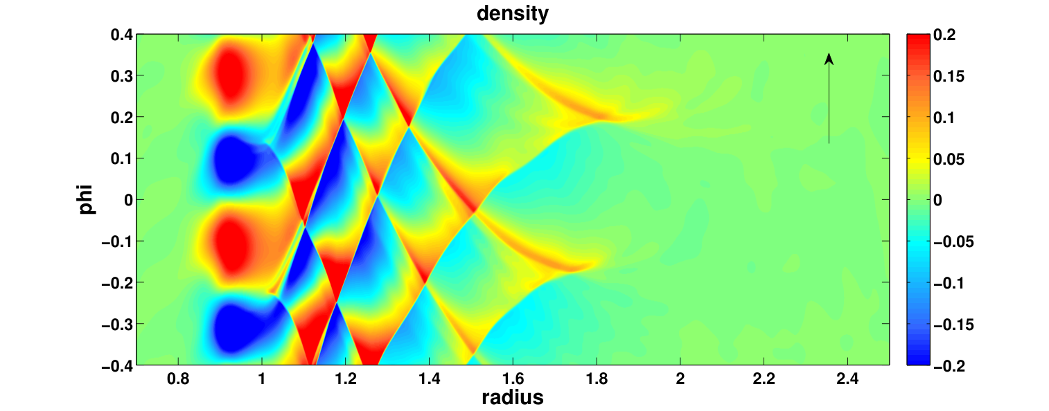

We now consider in more detail the structure of intersecting shocks caused by supersonic flow of disk material over the surface of the star. Since the shocks are weak, we can apply linear theory to study their properties. In the linear approximation, the dispersion relation for a normal mode perturbation of the form
| (18) |
is given by
| (19) |
which is simply the WKB dispersion relation for a fluid disk in the absence of self-gravity [9]. Here, is the radial wavenumber, is the azimuthal wavenumber, is the pattern speed, and is the epicyclic frequency.
For a given pattern speed , the right hand side of equation (19) consists entirely of known quantities so the radial wavenumber as a function of radius is uniquely determined. There are two corotation resonances in the system, one of which is located inside the boundary layer with the other one located inside the disk. Each of the two corotation resonances is flanked by two Lindblad resonances which occur at . In between a pair of Lindblad resonances, is imaginary (equation [19]), and these regions are forbidden to propagating waves, i.e. the waves are evanescent there.
It should be noted that the WKB approximation, which assumes breaks down near the Lindblad resonances, since at a Lindblad resonance. Nevertheless, we find that the WKB approximation works well in the disk, even near a Lindblad resonance. On the other hand, it performs poorly within the boundary layer, perhaps because the WKB approximation ignores radial density gradients which are large within the BL. For this reason, we will use a Keplerian rotation profile, , rather than using profiles for and determined from the simulations. A Keplerian profile is accurate inside the disk, and using it has the advantage of simplifying some of the analysis without compromising on the physics. For a Keplerian rotation profile, the corotation resonance in the disk is located at
| (20) |
and the Lindblad resonances are located at
| (21) |
When a shock launched from the BL encounters the forbidden region in the disk between the two Lindblad resonances, it is partially reflected back towards the BL. Moreover, this reflection is nearly perfect, and the transmission coefficient through the forbidden region is small - so small that it cannot be measured in the simulations. The reflected shock then propagates inward and is reflected again within the BL. The reflection within the BL could either be due to the presence of Lindblad and corotation resonances within the BL or because the radial scale height within the BL becomes smaller than the radial wavelength of the shock, i.e. . This process of reflections repeats cyclically resulting in a trapped mode between the BL and the forbidden region in the disk.
We point out that although the trapped modes are acoustic in nature, they are distinct from the sonic instabilities described in §III.1. First, the sonic instabilities saturate very early in the simulations (), whereas the trapped modes only develop much later around . The likely reason for this is that the boundary layer must settle down from the violent initial state that occurs when the sonic instabilities saturate before the trapped modes can develop. Second, there is clear leakage of wave action past the critical layer during the sonic instability phase (e.g. Figure 2), which is unbalanced by the wave dissipation, resulting in growth of the wave amplitude. At the same time, during the trapped mode phase wave action tunneling past the corotation region is not so noticeable (e.g. Figure 4). As a result, a quasi-steady state is established during this phase of evolution, and the trapped modes are stable for hundreds of orbital periods.
The black line in Figure 4b is the solution for an outgoing shock according to the dispersion relation (19) assuming a Keplerian rotation curve for and using . Due to the periodic boundary conditions in the direction, the shock exits from the top of the box and comes out again from the bottom. From Figure 4b, it is clear that the analytic solution given by the black line traces the numerical solution for an outgoing shock front very well, confirming the validity of the WKB approximation. As a sanity check we confirmed that the value of was consistent with a movie of the simulation.
The dashed vertical lines in Fig. 4b show the location of the inner and outer Lindblad resonances, which are located at and respectively, assuming . The solid vertical line is the corotation resonance, which is located at . In between the Lindblad resonances, in equation (19) is imaginary. This region is forbidden to propagating waves, and outgoing waves incident upon it are reflected back towards the boundary layer. The outgoing shock (yellow) traced by the black line in Fig. 4b is indeed seen to be reflected into an incoming shock (blue) in the vicinity of the inner Lindblad resonance.
III.3 Conservation of the Angular Momentum Flux
A prediction of linear theory that we confirm in our simulations is conservation of the angular momentum flux. In its most general form, the angular momentum flux for a disk with no self-gravity is given by
| (22) |
Proof that , i.e. that the angular momentum flux is conserved for stellar disks was first given by Toomre [50] using results about action density conservation from Whitham [54], Bretherton & Garrett [3].
For small perturbations away from axisymmetry (linear theory), the angular momentum flux is a second order quantity, and equation (22) becomes [9, 6, 47]
| (23) |
Here is the average surface density (equation [16]), and the overbar denotes a density-averaged quantity
| (24) |
The velocity perturbations and are given by
| (25) | |||||
| (26) |
We now test the linear theory during the quasi-steady state when there is a single mode rotating at a fixed pattern speed (§III.2). During the quasisteady state, we have outgoing shocks that undergo almost perfect reflection into incoming shocks at the Lindblad radius in the disk, so that . Thus rather than measuring , we instead measure the quantity
| (27) |
where the vertical lines denote taking the absolute value. Clearly, for nonzero perturbations. Moreover, away from shock crossings, when the outgoing and incoming shocks at a given radius are well-separated in azimuth, we have . This is because for well-separated shocks, measures the sum of the absolute values of the angular momentum flux carried by the individual outgoing and incoming shocks; the angular momentum flux is individually conserved for each of these shocks, implying that the sum of the absolute values of the angular momentum flux over all the shocks is also conserved.
In Appendix A, we demonstrate that sufficiently far from the Lindblad resonances (when ) and away from shock crossings, is related to the surface density perturbation (equation[17]) via
| (28) |
A similar result was previously obtained in the shearing-sheet approximation by Goodman & Rafikov [16].
Figure 5 shows from simulation A2 at , computed using equation (28) (solid line) and equation (27) (dashed line). It is not a problem that the simulation domain extends only from rather than the full in azimuth, since the boundary conditions are periodic and we can stack domains azimuthally. The arrows in the figure indicate the radii at which the two forms of are approximately equal. We have checked using Figure 4a that these radii correspond to regions which are in between shock crossings. In these regions, the individual shocks are well-separated in azimuth, which is precisely the regime under which equations (27) and (28) must give the same answer. When the shocks are not well-separated, equations (27) and (28) no longer agree, and the curves exhibit oscillations due to the presence of shock crossings. However, the two most important points are that away from the shock crossings: (1) equations (27) and (28) give similar values for , and (2) is roughly constant in radius with perhaps a slight, decreasing trend.
We see that between and , is roughly constant on average with periodic spikes, which correspond to shock crossings. This can be confirmed by matching the locations of the spikes in Figure 5 to the locations of the shock crossings in Figure 4, which shows images of the density and radial velocity at for simulation A2. Beyond the WKB approximation starts to break down, since we are near a resonance, and equation (28) underestimates the flux. Nevertheless, the fact that the curve is constant on average between and confirms that the angular momentum flux is conserved by the shocks.
We note that the angular momentum flux is not expected to be exactly conserved as the waves propagate since the shocks are not adiabatic and lose energy due to dissipation. However, accounting for the effect of dissipation on the angular momentum flux as a function of radius is made complicated by the fact that we have both outgoing and incoming (reflected) shocks in the simulation.
III.4 Effective Value of
It is common practice in semianalytic studies of the boundary layer to parametrize the angular momentum transport using an ad hoc prescription. Kley & Hensler [21], Popham & Narayan [38], Inogamov & Sunyaev [18], Piro & Bildsten [36], Balsara et al. [7] all used modified forms of the standard Shakura & Sunyaev [44] -viscosity prescription for disks, but the details of the prescription vary from one author to the next. The reason for such a lack of consensus comes from the fact that a simple -viscosity prescription leads to supersonic infall velocities in the BL, which Pringle [40] has argued are unphysical on the basis that the disk should remain causally connected to the star. Consequently, it is not clear how the angular momentum transport should be parametrized inside the BL, or whether it can be parametrized at all with a simple prescription, given the complicated shock structures that can develop.
In the purely hydrodynamical case, the starting point of any prescription for the angular momentum transport should be the Reynolds stress. We define the Reynolds stress as [6, 47]
| (29) |
From this, it is possible to define a dimensionless parameter
| (30) |
It is clear that is a dimensionless Reynolds stress, and this definition is consistent with the original definition of Shakura & Sunyaev [44]. However, one major point to keep in mind is that one should expect to be negative inside the BL. This is because the rotation profile rises in the BL () so angular momentum is transported inwards, spinning up the star. An inward transport of angular momentum, leads to a negative value of the Reynolds stress, and hence a negative value of .
Figure 6a shows a time-radius image of from simulation A2. It is evident that is negative and is spatially nonzero only in the vicinity of the BL (). The latter is due to the fact that we have no MRI in the disk and that shear instabilities only operate in the vicinity of the BL. It is also clear that is not constant in time, exhibiting temporal spikes at , , , and . We explain the reason for these spikes in §III.5. Typical maximum values of as a function of radius during the low and high accretion states (see §III.5 for the definition of low and high accretion state) are and respectively.
Figures 6b,c show time-radius images of the radial velocity, , and the mass accretion rate (equation [36]) within the disk. The radial velocity in the vicinity of the BL is predominantly negative and the mass accretion rate positive, indicating accretion onto the central object, and there are temporal spikes in the radial velocity and mass accretion rate that are coincident with the spikes in . In the disk proper outside the BL, the radial velocity exhibits alternating negative and positive regions, which are the imprints of the inward- and outward-propagating modes. In code units (§II), the typical values for the mean radial infall velocity during the low and high accretion states are and respectively, and typical values for the mass accretion rate during the low and high accretion states are and , respectively.


The negative value of the Reynolds stress in the BL yields a negative value of . It is straightforward, however, to define a parameter, , which one might expect to be positive in both the BL and the disk. We can do this through a prescription for the kinematic viscosity
| (31) |
where is the characteristic length scale for turbulent motions. The viscous stress is given by
| (32) |
and in the purely hydrodynamical case that we consider here, , since there are no magnetic stresses. Thus, we can write as
| (33) |
It is clear, then, that the condition for to be positive is that
| (34) |
and the stress should vanish at the location where .
For the value of in equation (33), we adopt the prescription of Popham & Narayan [38]
| (35) |
and we define , for purposes of readability. This prescription essentially sets the turbulent scale height to be the smaller of the vertical disk scale height, , and the radial pressure scale height, . This generalization is necessary for the BL, since the disk scale height defines the characteristic length scale inside the disk, whereas the pressure scale height defines it inside the star.
Figures 7 and 8 show the values of (equation [30]), (equation [33]), , and at (low state) and (high state) respectively. In each of the figures, both and have been averaged in time to reduce the level of fluctuations.
It is clear that is negative as discussed earlier, since the Reynolds stress is negative in the BL. On the other hand, is mostly positive in the boundary layer. However, the condition (34) is not exactly satisfied, leading to the large spike in Figs. 7b and 8b at and , respectively. Moreover, the rotation profile in the high state at is very flat between (Fig. 8c) and even contains a change in sign of (Fig. 8d). This again leads to a violation of condition (34) and leads to the densely packed spikes between in Fig. 8b.
If the non-trivial nature of the rotation profile (Figs. 7c and 8c) that we observe in our simplified simulations holds under astrophysical conditions, it seems unlikely that the dynamics of the BL can be captured with a simple prescription for . On the other hand, the dimensionless Reynolds stress is quite smooth and well-behaved inside the BL (Figs. 7a and 8a). Thus, could be the preferred parameter for constructing semi-analytical models of the BL.
III.5 High and Low Accretion States
From Figure 6 it is clear that our simulations are characterized by states of high and low accretion rate. The high accretion states are centered on , , , and and correspond to large absolute values of the Reynolds stress and of the radial infall velocity (Fig. 6). The low accretion state is relatively calm and is characterized by a single dominant mode that rotates at a constant pattern speed as discussed in §III.2. On the other hand, the oscillations of the interface during the high accretion state are more violent, and it becomes more difficult to determine a single dominant mode or a unique pattern speed. Nevertheless, the shock structure seen very distinctly in the low accretion state is still present to some extent even in the high accretion state. Fig. 9 shows a plot of the radial velocity in the high accretion state at for simulation A2, and can be compared with Fig. 4b, which shows the radial velocity during the low accretion state. It is clear that the high accretion state is more violent and chaotic than the low accretion state, but a dominant mode is still present.

We can understand the reason for transitioning from the low accretion state to the high accretion state by considering as a function of time. Fig. 10 shows at , 900, 1000, and 1100. These times span the duration of the third high accretion state in Fig. 6. We see that between and , a bump develops in the azimuthal velocity profile. This leads to a rapid rearrangement of the velocity profile between and , which erases the bump, and by the rearrangement of the velocity profile is complete.
The cause of the bump that appears in the profile are likely to be the oblique shocks present at the top of the BL. Each time a fluid element at the top of the BL passes through a shock, it is slowed down, and the collective effect of these shock passages creates the bump. Once the bump has been created, the mechanism for erasing it is the KH instability. KH instabilities can operate near inflection points in the velocity profile. At an inflection point, the radial derivative of the vorticity is constant, making it permissible to mix neighboring fluid elements and extract energy from the shear in the flow. In the vicinity of the bump, the vorticity profile is very flat, which allows the KH instability to operate there. Fig. 11 shows a snapshot of the vorticity () in the vicinity of the BL at , during the height of the high-accretion state. One can see that around , the vorticity is concentrated into structures that resemble the cats eye pattern associated with classical KH instabilities.

A curious point is that after a certain amount of time the system stops switching between high and low states and stays in the low state indefinitely. For instance, in Figure 6 it is clear that after four high-accretion states during which the system is in the high accretion state it stays in the low accretion state, until the end of the simulation. The cause of this behavior is unclear, but one should keep in mind that the inner part of the disk becomes more and more depleted of mass throughout the course of the simulation, see §III.6. If the material in the inner disk were replenished, as it would be in a real disk, the high accretion state might not shut off and continue to operate periodically.
It may be tempting to associate the high and low accretion states with the outburst and quiescent states of a CV. However, such a comparison is superficial given the fact that we are using an isothermal equation of state and have ignored magnetic fields. Nevertheless, the modification of the rotation profile by shocks and the subsequent onset of the KH instability is a very interesting phenomenon in its own right, even if it bears no relation to the mechanism causing outbursts in CVs.
III.6 Mass Accretion Due to Shocks
We confirm that even though we have purely hydrodynamical simulations, there is mass accretion onto the star. Figure 12 shows the density at and at for runs A5 and C1. From the figure, it is clear that the inner part of the disk has been evacuated at with material having been accreted onto the star. In Figure 12a, the innermost Lindblad radius is at . One can see that the depletion of mass occurs primarily inside of this radius, which is the region in which the trapped modes are present. There is some depletion even beyond this radius which is possibly due to the generation of a pressure gradient as mass in the inner region accretes. The gain in the radius of the star is more prominent for run A5 as opposed to run C1, for two reasons. First, the Mach number is two times lower in run A5 as compared to run C1 (6 vs 12), which means the radial scale height is four times smaller and the compression of accreted material larger in run C1. Second, more material has accreted at for run A5.
Most of the mass accretion in the simulations occurs during the high state, which is also when the Reynolds stress is largest. However, during the low accretion state, it is possible to “predict” the mass accretion rate in the disk based on the value of , and compare it to the “observed” accretion rate:
| (36) |
where the overbar represents an azimuthal density-weighted average.
To calculate the predicted mass accretion rate, we note that during the low accretion state there is a well-defined structure of shocks that rotates at a constant pattern speed. Given , one can use the fact that these shocks carry angular momentum, and because of dissipation, the angular momentum in the shock is transferred to the bulk flow driving accretion. In Appendix B, we derive an analytical expression for the mass accretion rate resulting from dissipation of weak shocks, given by equation (B7). We find that the mass accretion rates measured in our simulations using equation (36) agree to order of magnitude with the predicted mass accretion rates using equation (B7). For simulation A2, the mass accretion rate is (in our dimensionless units), during the low state around . This explains why the disk can persist for hundreds of orbital periods in the low state without being depleted. We note that during the high accretion state, the accretion rate can be much higher reaching values as high as in the boundary layer, where shear instabilities operate.
We also point out that accretion due to numerical viscosity is negligible in the simulations. For instance, in simulation A2, numerical viscosity gives rise to a numerical accretion rate of . This estimate was made by running a simulation with the same parameters as simulation A2, but without perturbations. In the absence of perturbations, the sonic instability does not set in, and we maintain an azimuthally-symmetric flow for the duration of the simulation, allowing us to measure the numerical mass accretion rate directly. We point out, however, that such an azimuthally-symmetric flow is grid-aligned in cylindrical coordinates. Thus, our measurement of the numerical mass accretion rate likely underestimates its true value in the science runs, where radial motions are present. Nevertheless, the fact that the accretion rate due to numerical viscosity in the grid-aligned case is three orders of magnitude lower than the measured accretion rate in the low-accretion state of simulation A2 provides convincing evidence that numerical viscosity is negligible in the simulations.
III.7 Stability of the Pattern Speed
Given that the system can transition between high and low states, one might wonder about the long-term stability of the modes discussed in §III.2. We find that the pattern speed in a given simulation stays constant to within a few percent over the course of hundreds of orbital periods. This is true even if the time interval in question contains transitions between high and low states. Figure 13 shows an image of the radial velocity for simulation A2 at time . This image can be compared with Figure 4b which is from the same simulation but was taken at . The pattern speed at is approximately , which is close to the pattern speed at of . Note that the interval of time between and contains two transitions from high accretion state to low accretion state.

III.8 Width of the BL
We plot the thickness of the BL defined by equation (15) as a function of time in Figure 14 for runs A1, A2, A3, B1, C1, and D1. The thickness of the BL greatly increases in the beginning of the simulation due to the sonic instabilities. It then stays approximately constant during the low accretion states and undergoes further changes during the high accretion states, eventually settling down to an approximately constant value. The fact that runs A1, A2, and A3 yield almost the same BL width at late times suggests that the simulations are converged, since these three runs differ only in their resolution.
It follows from Figure 10 that after significant evolution has taken place — typically after hundreds of orbital periods — the region in which azimuthal velocity transitions from the Keplerian profile to covers the radial interval . Thus, it extends both into the star and into the disk. This may have interesting implications for the morphology of the boundary layer in astrophysical systems.
It is clear from Figure 14 that the boundary layer becomes thinner with increasing Mach number. In Figure 15, we plot the width of the boundary layer at as a function of the Mach number on a log-log plot. The data point for is a simple average of simulations A1, A2, A3 and the points for , , and are from simulations B1, C1, and D1 respectively. The dashed line shows the best least squares fit to the data, and from its slope we deduce that , where is the width of the BL at . Since the scale height goes as (equation [10]), this indicates that the deceleration of the flow in the BL occurs over an approximately fixed number of scale heights in our simulations (), regardless of the Mach number.
IV Full Disk Simulations
Up until now, the simulations we have discussed have had a extent of radians. In this section, we consider global disk simulations, where the azimuthal angle runs from 0 to 2. This is important, since it is possible that the azimuthal wavenumber of the dominant global mode is of order unity. Lower azimuthal wavenumbers are inherently more interesting for explaining physical phenomena having frequencies less than or of order the orbital period at the surface of the star, such as DNOs. This is because the frequency of the mode is given by , and only if is low enough will also be low enough to provide a plausible explanation for such phenomena. Thus, we determine the azimuthal wavenumbers and pattern speeds of the dominant modes obtained from simulations in which goes from to .
Panels (a)-(d) of Figure 16 show images of the radial velocity from simulations A4, B2, C2, and D2, which have Mach numbers of and 15 respectively. These snapshots reveal a rather interesting structure of fluid perturbations, which is best seen at low values of . In particular, in panel (a), one can clearly discern a large-scale global mode along with some high frequency features, which are due to vortices at the base of the BL. There are more than 20 individual vortices that reside in the BL (where goes down from its Keplerian value in the disk to 0 in the star). Each of the vortices in the BL launches a shock into the disk, as discussed in §III.2, but now the individual shocks are superimposed on top of a global mode.
Thus, close inspection reveals two types of periodicities in our simulations — a large scale mode with relatively low wavenumber that extends out from the BL into the disk, and a set of periodic vortices contained in the BL with higher22 2 Note that in simulations presented in §III, which covered only a limited interval in it is generically found that (and typically equal to 2) since the azimuthal extent of the domain was setting the wavenumber of the mode. wavenumber ( in Figure 16a). The vortices at the base of the BL are only visible in panels (a) and to some extent of Figure 16. However, they are present as well in panels and and become apparent if the color scheme is saturated. The origin of the global mode is traced to a geometric resonance condition in §IV.1, but we leave the detailed investigation of the BL vortices to future study.
The pattern speed of the global mode in panel a of Figure 16 is . This is comparable to the pattern speed of the shock structure for simulation A2 discussed in §III.2, which has the same Mach number as simulation A4. The frequency of the mode is , and thus is lower but comparable to the orbital frequency at the inner radius of the disk.


IV.1 Relation of Pattern Speed to Azimuthal Wavenumber
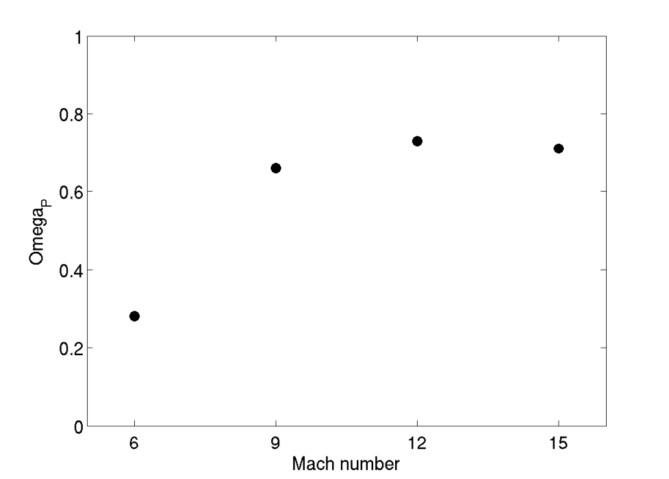
As the Mach number is increased, there is a general trend for the azimuthal wavenumber of the large scale pattern, , to increase as well. Figure 17a shows the wavenumber of the dominant global mode as a function of Mach number. We also plot the pattern speed as a function of Mach number in Figure 17b. There is again a general trend for the pattern speed to increase with increasing Mach number.
The dependence of the pattern speed on the azimuthal wavenumber of the global mode can be understood if we consider the total azimuthal angle traversed by a shock in traveling from the boundary layer to the inner Lindblad resonance in the disk and back. This angle is given by
| (37) |
and can be derived by using equation (19) together with the relation
| (38) |
which describes the trajectory along which the phase in equation (18) is constant. Here, and denote the boundary layer radius and the inner Lindblad radius in the disk, respectively. The factor of two out front comes from the fact that we are considering the total change in angle for a shock that starts from the boundary layer, is reflected at the Lindblad radius, and comes back to the boundary layer.
Formally we need to set equal to the location of the Lindblad resonance inside the BL. In practice, though, the shocks in our simulations are always observed to originate very near , and thus we simply set for the purposes of our calculations below.
An interesting question to ask is, given that we observe a mode with azimuthal wavenumber , what pattern speed would we predict based on equation (37), and how well does this predicted pattern speed match the observed pattern speed in our simulations? Assuming that the change in azimuthal angle for one “out and back” trip for the shock is given by equation (37), the condition that the shock pattern be closed is given by
| (39) |
where and are positive integers. It is natural to assume that , especially since the global modes don’t appear to overlap in Fig. 16 as they would if . For , an obvious choice to make is , since this naturally gives an -fold pattern. Thus, we postulate that
| (40) |
where is the azimuthal wavenumber of the global mode.
For simplicity, we assume a Keplerian rotation profile, in which case our estimate for becomes
| (41) |
where is given by equation (21). Assuming a Keplerian rotation profile gives a value of which is slightly larger than observed in the simulations. For instance, see Fig. 4b and note in particular that around , the shock profile becomes less steep than the analytic prediction using a Keplerian profile (black curve), due to the fact that the angular velocity is sub-Keplerian in that region. However, using the values of and is complicated by the fact that the WKB approximation breaks down in the boundary layer, (see §III.2 for a more detailed discussion).
The open circles in Fig. 18 show the value of that gives the correct value of (equation 40) using the formula (41) for the -numbers observed in the simulations. Conversely, the solid circles in Fig. 18 show the values of as measured from the simulations. We find that the predicted value of is within of the value observed in simulations and is always larger than the observed value. The latter point can be explained by the fact that using a Keplerian profile results in a larger value of as explained above. A smaller value of would lower the predicted value of , bringing the analytical predictions into closer agreement with the simulation results.
The good agreement between the predicted and observed pattern speeds over a range of Mach numbers suggests that there is a direct relation between the -number of the global modes in the disk and the pattern speed. This relation is essentially the combination of a periodicity condition and the dispersion relation for the modes.

V Discussion
The primary result of this work is the identification of a novel mechanism of angular momentum and mass transport in the boundary layer relying on non-axisymmetric acoustic modes which are generically excited in highly supersonic shear layers. Dissipation of these modes in weak shocks drives the evolution of the system and ultimately results in the mass transfer from the disk into the star. Our work is exploratory in nature and necessarily makes a number of simplifying assumptions, many of which are discussed in §V.2. Nevertheless we expect the main qualitative features of the new transport mechanism to persist also in more realistic settings typical for astrophysical boundary layers. The basic reason for this expectation lies in the fact that essentially the only ingredient necessary for the generation of acoustic modes is the presence of supersonic shear which is natural in astrophysical BLs.
Previously a number of hydrodynamical and MHD instabilities — Kelvin-Helmholtz, baroclinic, Tayler-Spruit dynamo [20, 12, 49, 46, 36, 19] have been invoked to drive the angular momentum transport in the BL. However, none of these instabilities were actually shown to operate under the conditions typical for the BL, where the supersonic nature of the flow is crucial for the dynamics and can drastically change the way in which these classical instabilities (usually explored in incompressible limit) operate. Armitage [1] and Steinacker & Papaloizou [47] have run direct 3D MHD simulations of BLs at a resolution that although state of the art at the time is low compared to the current simulations - their typical resolution in the radial direction is about an order of magnitude lower than in our work. These authors found that magnetic field amplification and mass accretion took place in the BL. However, whether the latter is due to the magnetic stresses and not due to the hydrodynamical effects like the one discussed here is not obvious. Transport induced by acoustic modes does not require magnetic field to be present in the first place, which makes this mechanism quite universal.
As part of our work we also looked at the linear stage of the sonic instability (see §III.1), which was previously explored under a more limited set of assumptions by Belyaev & Rafikov [8]. In particular, Belyaev & Rafikov [8] neglected the Coriolis force in their calculations and worked in Cartesian geometry. Despite that, their main results are in agreement with our more general calculations run in cylindrical geometry which fully account for the effects of rotation. This concordance justifies the simplifications made by Belyaev & Rafikov [8] in studying the sonic instability.
V.1 Variability in the BL
Because of the periodic nature of the trapped modes and their stability over many orbital periods, one may wonder whether they can produce a periodic modulation of the disk-star luminosity. One natural application of such a modulation is to the variability observed during the dwarf novae outbursts. The leading explanation for this variability involves magnetically-channeled accretion, which spins up an equatorial belt on the primary [32, 53]. An alternate explanation, and one that is relevant to our results is in terms of modes excited on the surface of the WD.
Papaloizou & Pringle [33] found that global non-axisymmetric modes excited in the surface layers would have the correct periods to account for DNOs. Later Popham [39] studied the possibility that DNOs could be caused by a bulge in the BL and Piro & Bildsten [37] considered shallow water modes in a BL that had spread meridionally to high latitudes. However, one of the main impediments to such theories is identifying the physical mechanism that would excite such surface modes in the first place.
If the picture of sonic instabilities leading to trapped modes that we have presented here remains valid even when additional physics is included (e.g. 3D nature of the flow, realistic cooling, effects of magnetic fields), then it would provide a mechanism for exciting surface modes. Since the frequency of DNOs is typically less than the orbital frequency at the surface of the star, the most favorable scenario for this mechanism to explain DNOs would involve a low number azimuthal mode . This is because one might expect a high -number mode to produce a small signal due to integrating the light over a hemisphere of the star. Also, the criterion that the DNO frequency be less than the orbital frequency at the surface of the star means that cannot be too large otherwise the criterion will not be fulfilled.
The only one of our simulations to satisfy the constraint is simulation A4 () with the higher Mach number simulations — more typical for realistic astrophysical systems — producing values of that are too high for DNOs. However, a detailed comparison to DNOs is premature at this point given the exploratory nature of the simulations - 2D with isothermal equation of state.
V.2 Extensions
We have performed 2D hydrodynamical simulations of the boundary layer and have found excitation of non-axisymmetric surface modes by the sonic instability. One may wonder how relevant our results are to real 3D disks with magnetic fields. We plan to address this question with future simulations, but for now we comment on what we expect may change in going from 2D hydro to 3D MHD simulations.
We have carried out some preliminary calculations to demonstrate the fundamental difference between the 2D and 3D cases and show the results in Figure 19. Panel (a) of Figure 19 corresponds to simulation A1 at time . Panel (b) is for a 3D simulation in cylindrical geometry with identical parameters except: the simulation domain has a vertical extent of (i.e. , where is the disk scale height), and there are 64 cells in the -direction. We use a cylindrical potential of the form , where is again the cylindrical radius, so the disk is unstratified. The boundary condition in the -direction is periodic for the 3D simulation.
The shock structure and the vortices at the base of the BL are clearly visible in Figure 19a, but are absent or only barely present in Figure 19b. Instead, in 3D the vortices at the base of the BL have been replaced by turbulence. We will explore the appearance of vortices at the base of the BL in a future work, but we remark here that the appearance of vortices could depend on the aspect ratio of the BL. If the BL has a vertical extent which is small compared to its radial extent, then one might expect vortices to be present, whereas if the BL has a vertical extent which is thick compared to its radial extent, then it may instead be turbulent. Nevertheless, the structure of intersecting shocks is still present in the disk even in the 3D case with turbulence (Figure 19b), although it is less clear cut than in the 2D case with vortices. One may also expect that the large-scale global modes discussed in §IV would not be affected by the turbulence, since the periodicity of global modes is determined by the geometric resonance condition (40). This does not involve the physics of what goes on inside the BL, which occurs on scales that are small compared to the wavelength of the global modes.
Additional effects may emerge in 3D hydrodynamical calculations in which vertical stratification in the disk is properly accounted for. Lubow & Ogilvie [26] and Bate et al [2] have demonstrated that waves in thermally stratified disks tend to propagate in such a way that their action density is concentrated predominantly near the disk surface, which increases wave amplitude and leads to faster nonlinear damping. In our case this effect may influence the damping of the trapped modes leading to their faster dissipation. Another important aspect of stratified 3D simulations is that they would allow one to naturally explore the spreading of material on the stellar surface towards high altitudes, resulting in formation of a spreading layer [18, 19].


One may also wonder how the addition of a magnetic field would modify our results. The BL is linearly stable to the MRI, since it has a rising rotation profile (). Nevertheless, due to the large shear present in the BL, a radial magnetic field can be kinematically sheared to produce a strong toroidal field. Armitage [1] and Steinacker & Papaloizou [47] found such an amplification in their simulations, but the field remained subthermal, and the magnetic energy density was only a fraction () of the thermal energy density in the boundary layer. This means that even in the MHD case, most of the pressure still comes from the gas, so one might expect the magnetic field and its associated pressure to only provide a small correction to the dispersion relation of the trapped modes.
Another way that MHD could affect the trapped modes is that the velocity fluctuations in the disk due to the MRI could be much larger than the velocity perturbations due to the shocks. Hawley et al. [17] found that the velocity fluctuations due to the MRI were of the sound speed in the disk. This is comparable to the velocity perturbation induced by the trapped modes in the disk. Thus one might expect that the trapped modes will have their wavefronts deformed by the MRI turbulence, but that the overall shock structure will still survive.
VI Conclusion
We have performed 2D hydrodynamic simulations of the boundary layer that self-consistently forms when the accretion disk is brought into contact with the stellar surface. Our calculations are restricted to the equatorial plane of the star+disk system which does not allow us to resolve the disk vertically but, quite importantly, captures the non-axisymmetric structures that emerge as a result of evolution. In our simulations, we used an isothermal equation of state and a Keplerian rotation profile inside the disk. We varied the Mach number at the inner edge of the disk to study how it affected the outcome of the simulations.
We find that sonic instabilities set in very rapidly in the interfacial region of large, supersonic shear between the star and the disk and saturate within a few orbital periods. After saturation, the initially thin boundary layer region expands radially both into the star and into the disk, with its final thickness depending on the Mach number as . This scaling implies that the boundary layer spans the same number of pressure scale heights () in our isothermal simulations independent of the Mach number.
After orbital periods, a trapped mode develops between the BL and a forbidden region in the disk, which consists of a corotation resonance flanked by two Lindblad resonances. The trapped mode is actually a weak shock (relative density perturbation ), and one can think of it as a global acoustic wave that alternately reflects off the BL and the forbidden region in the disk. The origin of this mode is intimately related to wave tunneling through the forbidden region and the associated phenomenon of overreflection. This trapped mode can persist for hundreds of orbital periods at a well defined pattern speed, . Both the pattern speed and azimuthal wavenumber of the the mode increase with increasing Mach number, and one can express the pattern speed in terms of the azimuthal wavenumber using a geometric resonance condition.
The trapped modes and initial sonic instabilities are able to drive accretion onto the star via dissipation in weak shocks even in the absence of magnetic fields. The steady state consisting of a trapped mode rotating at a given pattern speed can be interrupted by high-accretion states that are possibly caused by KH instability in the BL due to modification of the rotation profile by shocks. The non-axisymmetric nature of the acoustic modes found in our calculations gives rise to variability of the emission produced in the BL, which may be relevant for explaining phenomena such as dwarf novae oscillations in cataclysmic variables.
References
- [1] Armitage, P. J. 2002, MNRAS, 330, 895
- [2] Bate, M. R., Ogilvie, G. I., Lubow, S. H., & Pringle, J. E. 2002, MNRAS, 332, 575
- [3] Bretherton, F. P., & Garrett, C. J. R. 1968, Royal Society of London Proceedings Series A, 302, 529
- [4] Balbus, S. A. & Hawley, J. F. 1991a, ApJ, 367, 214
- [5] Balbus, S. A. & Hawley, J. F. 1991b, ApJ, 367, 223
- [6] Balbus, S. A., & Papaloizou, J. C. B. 1999, ApJ, 521, 650
- [7] Balsara, D. S., Fisker, J. L., Godon, P., & Sion, E. M. 2009, ApJ, 702, 1536
- [8] Belyaev, M. A., & Rafikov, R. R. 2012, ApJ, accepted, arxiv:1112.3102
- [9] Binney, J., & Tremaine, S. 2008, Galactic Dynamics: Second Edition, by James Binney and Scott Tremaine. ISBN 978-0-691-13026-2 (HB). Published by Princeton University Press, Princeton, NJ USA, 2008.
- [10] Bruch, A. 2000, A&A, 359, 998
- [11] Chandrasekhar, S. 1960, Proc. Natl. Acad. Sci., 46, 253
- [12] Fujimoto, M. Y. 1993, ApJ, 419, 768
- [13] Glatzel, W. 1988, MNRAS, 231, 795
- [14] Goldreich, P., & Tremaine, S. 1978, ApJ, 222, 850
- [15] Goldreich, P., & Tremaine, S. 1979, ApJ, 233, 857
- [16] Goodman, J., & Rafikov, R. R. 2001, ApJ, 552, 793
- [17] Hawley, J. F., Gammie, C. F., & Balbus, S. A. 1995, ApJ, 440, 742
- [18] Inogamov, N. A., & Sunyaev, R. A. 1999, Astronomy Letters, 25, 269
- [19] Inogamov, N. A. & Sunyaev, R. A. 2010, Ast. Let., 36, 848
- [20] Kippenhahn, R. & Thomas, H.-C. 1978, A&A, 63, 265
- [21] Kley, W., & Hensler, G. 1987, A&A, 172, 124
- [22] Kluźniak, W. 1987, Ph.D. Thesis
- [23] Landau, L. D., & Lifshitz, E. M. 1959, Course of theoretical physics, Oxford: Pergamon Press, 1959
- [24] Larson, R. B. 1990, MNRAS, 243 588
- [25] Livio, M., & Pringle, J. E. 1992, MNRAS, 259, 23P
- [26] Lubow, S. H. & Ogilvie, G. I. 1998, ApJ, 504, 983
- [27] Lynden-Bell, D., & Pringle, J. E. 1974, MNRAS, 168, 603
- [28] Mark, J. W-K. 1976, ApJ, 205, 363
- [29] Meyer, F. & Meyer-Hofmeister, E. 1994, A&A, 288, 175
- [30] Narayan, R., & Popham, R. 1993, Nature, 362, 820
- [31] Narayan, R., Goldreich, P., & Goodman, J. 1987, MNRAS, 228, 1
- [32] Paczyński, B. 1978, Nonstationary Evolution of Close Binaries, 89
- [33] Papaloizou, J., & Pringle, J. E. 1978, MNRAS, 182, 423
- [34] Papaloizou, J. C. B., & Pringle, J. E. 1984, MNRAS, 208, 721
- [35] Patterson, J. 1981, ApJS, 45, 517
- [36] Piro, A. L., & Bildsten, L. 2004, ApJ, 610, 977
- [37] Piro, A. L., & Bildsten, L. 2004, ApJ, 616, L155
- [38] Popham, R., & Narayan, R. 1995, ApJ, 442, 337
- [39] Popham, R. 1999, MNRAS, 308, 979
- [40] Pringle, J. E. 1977, MNRAS, 178, 195
- [41] Pringle, J. E., & Savonije, G. J. 1979, MNRAS, 187, 777
- [42] Rafikov, R. R. 2002, ApJ, 569, 997
- [43] Romanova, M. M., Ustyugova, G. V., Koldoba, A. V., & Lovelace, R. V. E. 2011, arXiv:1111.3068
- [44] Shakura, N. I., & Sunyaev, R. A. 1973, A&A, 24, 337
- [45] Skinner, M. A., & Ostriker, E. C. 2010, ApJS, 188, 290
- [46] Spruit, H. C. 2002, A&A, 381, 923
- [47] Steinacker, A., & Papaloizou, J. C. B. 2002, ApJ, 571, 413
- [48] Stone, J. M., Gardiner, T. A., Teuben, P., Hawley, J. F., & Simon, J. B. 2008, ApJS, 178, 137
- [49] Tayler, R. J. 1973, MNRAS, 161, 365
- [50] Toomre, A. 1969, ApJ, 158, 899
- [51] Velikhov, E. P. 1959 J. Exptl. Theoret. Phys., 36, 1398
- [52] Warner, B. 2004, PASP, 116, 115
- [53] Warner, B., & Woudt, P. A. 2002, MNRAS, 335, 84
- [54] Whitham, G. B. 1965, Journal of Fluid Mechanics, 22, 273
- [55] Zingale, M., Dursi, L. J., ZuHone, J., et al. 2002, ApJS, 143, 539
Appendix A Angular Momentum Flux from a Superposition of Modes
In the WKB limit (), the angular momentum flux for a normal mode with azimuthal wavenumber becomes
| (A1) |
(see Goldreich & Tremaine [15] and Appendix J of Binney & Tremaine [9]). Here is the radial wavenumber and determines the direction of angular momentum transport, inward or outward. The Fourier coefficient in equation (A1) is defined such that an arbitrary density perturbation, , can be expressed as a sum over Fourier components having :
| (A2) |
Since the shocks in our simulations are not perfect normal modes, we need to compute the angular momentum flux for an arbitrary density profile with a given pattern speed. This can be done by summing over the angular momentum transported by the individual modes so we have
| (A3) |
Note that the term does not contribute to angular momentum transport, which can be seen from equation (A1). This point allows us to perform a mathematical trick that will simplify the analysis. Since the mode does not contribute to the total angular momentum transported flux, we are free to set it to zero in equation (A2). Although this has an effect on the density profile, it does not change the total angular momentum flux.
Setting the component of the density profile to zero, we can rewrite equation (A2) as
| (A4) |
where . Parseval’s theorem, which we shall shortly invoke, can then be written as
| (A5) |
Using Parseval’s theorem, we now derive an approximate formula for computing the angular momentum flux that does not involve summing over the individual Fourier coefficients as in equation (A3). We begin by making the assumption ( for Keplerian profile) so that the expression for (Eq. 19) simplifies to
| (A6) |
where . Consequently, this assumption is true if , and we are far away from any resonances so that .
Substituting equation (A6) into equation (A1), we have for the angular momentum flux due to a given mode
| (A7) |
The total angular momentum flux from equation (A3) is given by
| (A8) |
We shall assume that for a given shock, all of the modes have the same sign of , i.e. the shock is either incoming or outgoing. This is a reasonable assumption except near shock crossings, where incoming and outgoing shocks having opposite signs for interact. For a given shock, this allows us to take out of the summation sign, assuming the individual shocks are azimuthally well-separated. Since is the sum of the absolute values of the angular momentum flux for the individual shocks, assuming the shocks are well-separated, we arrive at
| (A9) |
Here we have assumed which is true for the trapping region between the boundary layer and the Lindblad resonance in the disk. Using Parseval’s theorem, equation (A9) becomes equation (28).
Appendix B Mass Accretion Rate Due to Weak Shocks.
The mass accretion rate through the disk can be expressed through the divergence of the angular momentum flux deposited in the disk fluid by the waves (or acoustic modes) due to their dissipation at the shock fronts [27]
| (B1) |
where is the specific angular momentum for circular orbits. The subsequent derivation is based in part on the work by Larson [24].
The modes are stationary in a frame rotating with angular speed . Excitation of a wavepacket carrying angular momentum requires energy . Dissipation of this wavepacket at some other radial distance transfers angular momentum to the disk fluid — a process which is necessarily accompanied by the mechanical work being done on the disk. The rest of energy, , is available for heating the disk and is ultimately radiated away.
Thus, if the dissipation of the wave adds angular momentum to the disk fluid at the rate per unit of (the radial divergence of the wave angular momentum flux due to the wave damping), then the local tidal energy dissipation rate is given by
| (B2) |
See Goodman & Rafikov [16] for the discussion of this issue.
It is difficult to calculate from first principles. However, one can compute and use equation (B2) to obtain . The reason behind using this approach is that dissipation along a given fluid element’s trajectory occurs only at the shocks (unlike azimuthal acceleration and deceleration due to pressure gradients that occurs also between the shocks) — between the shocks the flow is adiabatic (in the absence of numerical dissipation).
For weak shocks Larson [24] gives the amount of energy irreversibly turned into heat at the shock per unit mass of the fluid crossing the shock as
| (B3) |
where Landau & Lifshitz [23]
| (B4) |
is the Mach number of the weak shock, is the density contrast across the shock, and is the sound speed. For an isothermal shock () the expression is exact. Thus, for we have
| (B5) |
Now, in an annulus of width the mass crosses one of the shocks (the factor of 2 comes from accounting for both inward- and outward-propagating waves) per time , so that
| (B6) |
meaning that . Finally,
| (B7) |
If we define the “local disk mass” to be then the accretion timescale becomes (for )
| (B8) |
where is the Mach number of the flow.
If the disk were a disk then , where is the “effective” -viscosity due to trapped shocks. Combining this with equation (B7) one gets
| (B9) |
in agreement with Larson [24].