Diffusion Strategies Outperform Consensus Strategies for Distributed Estimation over Adaptive Networks

Sheng-Yuan Tu Ali H. Sayed ^†^†thanks: Copyright (c) 2012 IEEE. Personal use of this material is permitted. However, permission to use this material for any other purposes must be obtained from the IEEE by sending a request to pubs-permissions@ieee.org.^†^†thanks: This work was supported in part by NSF grants CCF-1011918 and CCF-0942936. An earlier version of this work appeared in [1]. The authors are with the Department of Electrical Engineering, University of California, Los Angeles (e-mail: shinetu@ee.ucla.edu; sayed@ee.ucla.edu).

Abstract

Adaptive networks consist of a collection of nodes with adaptation and learning abilities. The nodes interact with each other on a local level and diffuse information across the network to solve estimation and inference tasks in a distributed manner. In this work, we compare the mean-square performance of two main strategies for distributed estimation over networks: consensus strategies and diffusion strategies. The analysis in the paper confirms that under constant step-sizes, diffusion strategies allow information to diffuse more thoroughly through the network and this property has a favorable effect on the evolution of the network: diffusion networks are shown to converge faster and reach lower mean-square deviation than consensus networks, and their mean-square stability is insensitive to the choice of the combination weights. In contrast, and surprisingly, it is shown that consensus networks can become unstable even if all the individual nodes are stable and able to solve the estimation task on their own. When this occurs, cooperation over the network leads to a catastrophic failure of the estimation task. This phenomenon does not occur for diffusion networks: we show that stability of the individual nodes always ensures stability of the diffusion network irrespective of the combination topology. Simulation results support the theoretical findings.

Index Terms:

Adaptive networks, diffusion strategy, consensus strategy, mean stability, mean-square stability, mean-square-error performance, combination weights.

I Introduction

Adaptive networks consist of a collection of spatially distributed nodes that are linked together through a topology and that cooperate with each other through local interactions. Adaptive networks are well-suited to perform decentralized information processing and inference tasks [2, 3] and to model complex and self-organized behavior encountered in biological systems [4, 5].

We examine two types of fully decentralized strategies, namely, consensus strategies and diffusion strategies. The consensus strategy was originally proposed in the statistics literature [6] and has since then been developed into an elegant procedure to enforce agreement among cooperating nodes. Average consensus and gossip algorithms have been studied extensively in recent years, especially in the control literature [7, 8, 9, 10, 11, 12], and applied to the study of multi-agent formations [13, 14], distributed optimization [15, 16], and distributed estimation problems [17, 18, 19]. Original implementations of the consensus strategy relied on the use of two time-scales [20, 21, 22]: one time-scale for the collection of measurements across the nodes and another time-scale to iterate sufficiently enough over the collected data to attain agreement before the process is repeated. Unfortunately, two time-scale implementations hinder the ability to perform real-time recursive estimation and adaptation when measurement data keep streaming in. For this reason, in this work, we focus instead on consensus implementations that operate in a single time-scale. Such implementations appear in several recent works, including [16, 19, 17, 18], and are largely motivated by the procedure developed earlier in [15, 23] for the solution of distributed optimization problems.

The second class of algorithms that we consider deals with diffusion strategies, which were originally introduced for the solution of distributed estimation and adaptation problems in [24, 25, 26, 2, 3]. The main motivation for the introduction of diffusion strategies in these works was the desire to develop distributed schemes that are able to respond in real-time to continuous streaming of data at the nodes by operating over a single time-scale. A useful overview of diffusion strategies appears in [27]. Since their inception, diffusion strategies have been applied to model various forms of complex behavior encountered in nature [4, 5]; they have also been adopted to solve distributed optimization problems advantageously in [28, 29, 30]; and have been studied under varied conditions in [31, 32, 33, 34] as well. Diffusion strategies are inherently single time-scale implementations and are therefore naturally amenable to real-time and recursive implementations. It turns out that the dynamics of the consensus and diffusion strategies differ in important ways, which in turn impact the mean-square behavior of the respective networks in a fundamental manner.

The analysis in this paper will confirm that under constant step-sizes, diffusion strategies allow information to diffuse more thoroughly through networks and this property has a favorable effect on the evolution of the network. It will be shown that diffusion networks converge faster and reach lower mean-square deviation than consensus networks, and their mean-square stability is insensitive to the choice of the combination weights. In comparison, and surprisingly, it is shown that consensus networks can become unstable even if all the individual nodes are stable and able to solve estimation task on their own. In other words, the learning curve of a cooperative consensus network can diverge even if the learning curves for the non-cooperative individual nodes converge. When this occurs, cooperation over the network leads to a catastrophic failure of the estimation task. This behavior does not occur for diffusion networks: we will show that stability of the individual nodes is sufficient to ensure stability of the diffusion network regardless of the combination weights. The properties revealed in this paper indicate that there needs to be some care with the use of consensus strategies for adaptation because they can lead to network failure even if the individual nodes are stable and well-behaved. The analysis also suggests that diffusion strategies provide a proper way to enforce cooperation over networks; their operation is such that diffusion networks will always remain stable irrespective of the combination topology.

II Estimation Strategies over Networks

Consider a network consisting of $N$ nodes distributed over a spatial domain. Two nodes are said to be neighbors if they can exchange information. The neighborhood of node $k$ is denoted by $\mathcal{N}_{k}$ . The nodes in the network would like to estimate an unknown $M\times 1$ vector, $w^{\circ}$ . At every time instant, $i$ , each node $k$ is able to observe realizations $\{d_{k}(i),u_{k,i}\}$ of a scalar random process $\boldsymbol{d}_{k}(i)$ and a $1\times M$ vector random process $\boldsymbol{u}_{k,i}$ with a positive-definite covariance matrix, $R_{u,k}=\mathbb{E}\boldsymbol{u}_{k,i}^{*}\boldsymbol{u}_{k,i}>0$ , where $\mathbb{E}$ denotes the expectation operator. All vectors in our treatment are column vectors with the exception of the regression vector, $\boldsymbol{u}_{k,i}$ , which is taken to be a row vector for convenience of presentation. The random processes $\{\boldsymbol{d}_{k}(i),\boldsymbol{u}_{k,i}\}$ are related to $w^{\circ}$ via the linear regression model [35]:

\boldsymbol{d}_{k}(i)=\boldsymbol{u}_{k,i}w^{\circ}+\boldsymbol{v}_{k}(i)

(1)

where $\boldsymbol{v}_{k}(i)$ is measurement noise with variance $\sigma^{2}_{v,k}$ and assumed to be temporally white and spatially independent, i.e.,

\mathbb{E}\boldsymbol{v}^{*}_{k}(i)\boldsymbol{v}_{l}(j)=\sigma^{2}_{v,k}\cdot\delta_{kl}\cdot\delta_{ij}

(2)

in terms of the Kronecker delta function. The regression data $\boldsymbol{u}_{k,i}$ are likewise assumed to be temporally white and spatially independent. The noise $\boldsymbol{v}_{k}(i)$ and the regressors $\{\boldsymbol{u}_{l,j}\}$ are assumed to be independent of each other for all $\{k,l,i,j\}$ . All random processes are assumed to be zero mean. Note that we use boldface letters to denote random quantities and normal letters to denote their realizations or deterministic quantities. Models of the form (1) are useful in capturing many situations of interest, such as estimating the parameters of some underlying physical phenomenon, tracking a moving target by a collection of nodes, or estimating the location of a nutrient source or predator in biological networks (see, e.g., [4, 5, 35]); these models are also useful in the study of the performance limits of combinations of adaptive filters [36, 37, 38, 39].

The objective of the network is to estimate $w^{\circ}$ in a distributed manner through an online learning process. The nodes estimate $w^{\circ}$ by seeking to minimize the following global cost function:

J^{\text{glob}}(w)\triangleq\sum_{k=1}^{N}\mathbb{E}|\boldsymbol{d}_{k}(i)-\boldsymbol{u}_{k,i}w|^{2}.

(3)

In the sequel, we describe the algorithms pertaining to the consensus and diffusion strategies that we study in this article, in addition to the non-cooperative mode of operation. Afterwards, we move on to the main theme of this work, which is to show why diffusion networks outperform consensus networks. We may remark that the same strategies can be used to optimize global cost functions where the individual costs are not necessarily quadratic in $w$ as in (3). Most of the mean-square analysis performed here can be extended to this more general scenario — see, e.g., [30, 40] and the references therein.

II-A Non-Cooperative Strategy

In the non-cooperative mode of operation, each node $k$ operates independently of the other nodes and estimates $w^{\circ}$ by means of a local LMS adaptive filter applied to its data $\{d_{k}(i),u_{k,i}\}$ . The filter update takes the following form [41, 35]:

\text{(non-cooperative strategy)}\quad\boxed{w_{k,i}=w_{k,i-1}+\mu_{k}u_{k,i}^{*}[d_{k}(i)-u_{k,i}w_{k,i-1}]}

(4)

where $\mu_{k}>0$ is the constant step-size used by node $k$ . In (4), the vector $w_{k,i}$ denotes the estimate for $w^{\circ}$ that is computed by node $k$ at time $i$ . Note that for the underlying model where $R_{u,k}>0$ for all $k$ , every individual node can employ (4) to estimate $w^{\circ}$ independently if desired. Studies allowing for other observability conditions for diffusion and consensus strategies, including possibly singular covariance matrices, appear in [18, 42].

II-B Cooperative Strategies

In the cooperative mode of operation, nodes interact with their neighbors by sharing information. In this article, we study three cooperative strategies for distributed estimation.

B.1. Consensus Strategy

The consensus strategy often appears in the literature in the following form (see, e.g., Eq. (1.20) in [16], Eq. (19) in [17], and Eq. (9) in [18]):

\displaystyle w_{k,i}=w_{k,i-1}-\mu_{k}(i)\cdot\sum_{l\in\mathcal{N}_{k}\setminus\{k\}}b_{l,k}(w_{k,i-1}-w_{l,i-1})+\mu_{k}(i)\cdot u_{k,i}^{*}[d_{k}(i)-u_{k,i}w_{k,i-1}]

(5)

where $\{b_{l,k}\}$ is a set of nonnegative coefficients. It should be noted that in most works on consensus implementations, especially in the context of distributed optimization problems [16, 23, 17, 18, 28], the step-sizes $\{\mu_{k}(i)\}$ that are used in (5) depend on the time-index $i$ and are required to satisfy

\sum_{i=0}^{\infty}\mu_{k}(i)=\infty\text{ and }\sum_{i=0}^{\infty}\mu_{k}^{2}(i)<\infty.

(6)

In other words, for each node $k$ , the step-size sequence $\mu_{k}(i)$ is required to vanish as $i\rightarrow\infty$ . Under such conditions, it is known that consensus strategies allow the nodes to reach agreement about $w^{\circ}$ [16, 18, 43, 44]. Here, instead, we will use constant step-sizes $\{\mu_{k}\}$ . This is because we are interested in studying the adaptation and learning abilities of the networks. Constant step-sizes are critical to endow networks with continuous adaptation and tracking abilities; otherwise, under (6), once the step-sizes have decayed to zero, the network stops adapting and learning is turned off.

We can rewrite recursion (5) in a more compact and revealing form by combining the first two terms on the right-hand side of (5) and by introducing the following coefficients:

a_{l,k}\triangleq\begin{cases}1-\sum_{j\in\mathcal{N}_{k}\setminus\{k\}}\mu_{k}b_{j,k},&\text{if $l=k$}\\ \mu_{k}b_{l,k},&\text{if $l\in\mathcal{N}_{k}\setminus\{k\}$}\\ 0,&\text{otherwise}\end{cases}

(7)

In this way, recursion (5) can be rewritten equivalently as (see, e.g., expression (7.1) in [23] and expression (1.20) in [16]):

\text{(consensus strategy)}\quad\boxed{w_{k,i}=\sum_{l\in\mathcal{N}_{k}}a_{l,k}w_{l,i-1}+\mu_{k}u_{k,i}^{*}[d_{k}(i)-u_{k,i}w_{k,i-1}]}

(8)

The entry $a_{l,k}$ denotes the weight that node $k$ assigns to the estimate $w_{l,i-1}$ received from its neighbor $l$ (see Fig. 1); note that the weights $\{a_{l,k}\}$ are nonnegative for $l\neq k$ and that $a_{k,k}$ is nonnegative for sufficiently small step-sizes. If we collect the nonnegative weights $\{a_{l,k}\}$ into an $N\times N$ matrix $A$ , then it follows from (7) that the combination matrix $A$ satisfies the following properties:

\boxed{a_{l,k}\geq 0\text{, }A^{T}\mathds{1}=\mathds{1}\text{, and }a_{l,k}=0\text{ if $l\notin\mathcal{N}_{k}$}}

(9)

where $\mathds{1}$ is a vector of size $N$ with all entries equal to one. That is, the weights on the links arriving at node $k$ add up to one, which is equivalent to saying that the matrix $A$ is left-stochastic. Moreover, if two nodes $l$ and $k$ are not linked, then their corresponding entry $a_{l,k}$ is zero.

Refer to caption — Fig. 1: A connected network showing the neighborhood of node $k$ , denoted by $\mathcal{N}_{k}$ . The weight $a_{l,k}$ scales the data transmitted from node $l$ to node $k$ over the edge linking them.

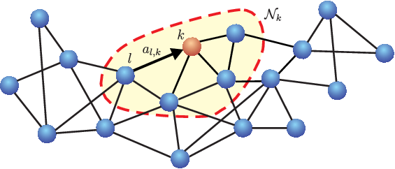
B.2. ATC Diffusion Strategy

Diffusion strategies for the optimization of (3) in a fully decentralized manner were derived in [24, 25, 2, 26, 3, 30] by applying a completion-of-squares argument, followed by a stochastic approximation step and an incremental approximation step — see [27]. The adapt-then-combine (ATC) form of the diffusion strategy is described by the following update equations [3]:

{}\text{(ATC diffusion strategy)}\quad\boxed{\begin{aligned} \psi_{k,i}&=w_{k,i-1}+\mu_{k}u_{k,i}^{*}[d_{k}(i)-u_{k,i}w_{k,i-1}]\\ w_{k,i}&=\sum_{l\in\mathcal{N}_{k}}a_{l,k}\psi_{l,i}\end{aligned}}.

(10)

The above strategy consists of two steps. The first step of (10) involves local adaptation, where node $k$ uses its own data $\{d_{k}(i),u_{k,i}\}$ to update its weight estimate from $w_{k,i-1}$ to an intermediate value $\psi_{k,i}$ . The second step of (10) is a consultation (combination) step where the intermediate estimates $\{\psi_{l,i}\}$ from the neighborhood of node $k$ are combined through weights $\{a_{l,k}\}$ that satisfy (9) to obtain the updated weight estimate $w_{k,i}$ .

B.3. CTA Diffusion Strategy

Another variant of the diffusion strategy is the combine-then-adapt (CTA) form, which is described by the following update equations [2]:

\text{(CTA diffusion strategy)}\quad\boxed{\begin{aligned} \psi_{k,i-1}&=\sum_{l\in\mathcal{N}_{k}}a_{l,k}w_{l,i-1}\\ w_{k,i}&=\psi_{k,i-1}+\mu_{k}u_{k,i}^{*}[d_{k}(i)-u_{k,i}\psi_{k,i-1}]\end{aligned}}.

(11)

Thus, comparing the ATC and CTA strategies, we note that the order of the consultation and adaptation steps are simply reversed. The first step of (11) involves a consultation step, where the existing estimates $\{w_{l,i-1}\}$ from the neighbors of node $k$ are combined through the weights $\{a_{l,k}\}$ . The second step of (11) is a local adaptation step, where node $k$ uses its own data $\{d_{k}(i),u_{k,i}\}$ to update its weight estimate from the intermediate value $\psi_{k,i-1}$ to $w_{k,i}$ .

B.4. Comparing Diffusion and Consensus Strategies

For ease of comparison, we rewrite below the recursions that correspond to the consensus (8), ATC diffusion (10), and CTA diffusion (11) strategies in a single update:

$\displaystyle\text{(consensus)}\quad w_{k,i}$	$\displaystyle=\sum_{l\in\mathcal{N}_{k}}a_{l,k}w_{l,i-1}+\mu_{k}u_{k,i}^{*}[d_{k}(i)-u_{k,i}w_{k,i-1}]$	(12)
$\displaystyle\text{(ATC diffusion)}\quad w_{k,i}$	$\displaystyle=\sum_{l\in\mathcal{N}_{k}}a_{l,k}\left(w_{l,i-1}+\mu_{l}u_{l,i}^{*}[d_{l}(i)-u_{l,i}w_{l,i-1}]\right)$	(13)
$\displaystyle\text{(CTA diffusion)}\quad w_{k,i}$	$\displaystyle=\sum_{l\in\mathcal{N}_{k}}a_{l,k}w_{l,i-1}+\mu_{k}u_{k,i}^{*}\left[d_{k}(i)-u_{k,i}\left(\sum_{l\in\mathcal{N}_{k}}a_{l,k}w_{l,i-1}\right)\right].$	(14)

Note that the first terms on the right hand side of these recursions are all the same. For the second terms, only variable $w_{k,i-1}$ appears in the consensus strategy (12), while the diffusion strategies (13)-(14) incorporate the estimates $\{w_{l,i-1}\}$ from the neighborhood of node $k$ into the update of $w_{k,i}$ . Moreover, in contrast to the consensus (12) and CTA diffusion (14) strategies, the ATC diffusion strategy (13) further incorporates the influence of the data $\{d_{l}(i),u_{l,i}\}$ from the neighborhood of node $k$ into the update of $w_{k,i}$ . These differences in the order by which the computations are performed have important implications on the evolution of the weight-error vectors across consensus and diffusion networks. It is important to note that the diffusion strategies (13)-(14) are able to incorporate additional information into their processing steps without being more complex than the consensus strategy. All three strategies have the same computational complexity and require sharing the same amount of data (see Table I), as can be ascertained by comparing the actual implementations (8), (10), and (11). The key fact to note is that the diffusion implementations first generate an intermediate state variable, which is subsequently used in the final update. This important ordering of the calculations has a critical influence on the performance of the algorithms, as we now move on to reveal.

TABLE I: Comparison of the number of complex multiplications and additions per iteration, as well as the number of

M\times 1

vectors that are exchanged for each iteration of the algorithms at every node

k

. In the table, the symbol

n_{k}

denotes the degree of node

k

, i.e., the size of its neighborhood

\mathcal{N}_{k}

. Observe that all three strategies have exactly the same computational complexity.

	ATC diffusion (10)	CTA diffusion (11)	Consensus (8)
Multiplications	$(n_{k}+2)M$	$(n_{k}+2)M$	$(n_{k}+2)M$
Additions	$(n_{k}+1)M$	$(n_{k}+1)M$	$(n_{k}+1)M$
Vector exchanges	$n_{k}$	$n_{k}$	$n_{k}$

III Mean-Square Performance Analysis

The mean-square performance of diffusion networks has been studied in detail in [2, 3, 27] by applying energy conservation arguments [35, 45]. Following [3], we will first show how to carry out the performance analysis in a unified manner that covers both diffusion and consensus strategies (see Table II further ahead, which highlights how the parameters for both strategies differ). Subsequently, we use the resulting performance expressions to carry out detailed comparisons and to establish and highlight some surprising and interesting differences in performance.

III-A Network Error Recursion

Let the error vector for an arbitrary node $k$ be denoted by

\tilde{\boldsymbol{w}}_{k,i}\triangleq w^{\circ}-\boldsymbol{w}_{k,i}.

(15)

We collect all error vectors and step-sizes across the network into a block vector and block matrix:

	$\displaystyle\tilde{\boldsymbol{w}}_{i}$	$\displaystyle\triangleq\text{col}\left\{\tilde{\boldsymbol{w}}_{1,i},\tilde{\boldsymbol{w}}_{2,i},\cdots,\tilde{\boldsymbol{w}}_{N,i}\right\}$		(16)
	$\displaystyle\mathcal{M}$	$\displaystyle\triangleq\text{diag}\{\mu_{1}I_{M},\mu_{2}I_{M},\cdots,\mu_{N}I_{M}\}$		(17)

where the notation $\text{col}\{\cdot\}$ denotes the vector that is obtained by stacking its arguments on top of each other, and the notation $\text{diag}\{\cdot\}$ constructs a diagonal matrix from its arguments. We further introduce the extended combination matrix:

\mathcal{A}\triangleq A\otimes I_{M}

(18)

where the symbol $\otimes$ denotes the Kronecker product of two matrices. This construction replaces each entry $a_{l,k}$ in $A$ by the $M\times M$ diagonal matrix $a_{l,k}I_{M}$ in $\mathcal{A}$ . Then, if we start from (12), (13), or (14), and use model (1), some straightforward algebra similar to [3, 27] shows that the global error vector $\tilde{\boldsymbol{w}}_{i}$ for the various strategies evolves according to the following recursion:

\boxed{\tilde{\boldsymbol{w}}_{i}=\boldsymbol{\mathcal{B}}_{i}\cdot\tilde{\boldsymbol{w}}_{i-1}-\boldsymbol{y}_{i}}

(19)

where the quantities $\boldsymbol{\mathcal{B}}_{i}$ and $\boldsymbol{y}_{i}$ are listed in Table II and where $\boldsymbol{\mathcal{R}}_{i}$ is a block diagonal matrix and $\boldsymbol{s}_{i}$ is a block column vector:

	$\displaystyle\boldsymbol{\mathcal{R}}_{i}$	$\displaystyle\triangleq\text{diag}\{\boldsymbol{u}^{}_{1,i}\boldsymbol{u}_{1,i},\boldsymbol{u}^{}_{2,i}\boldsymbol{u}_{2,i},\cdots,\boldsymbol{u}^{*}_{N,i}\boldsymbol{u}_{N,i}\}$		(20)
	$\displaystyle\boldsymbol{s}_{i}$	$\displaystyle\triangleq\text{col}\{\boldsymbol{u}^{}_{1,i}\boldsymbol{v}_{1,i},\boldsymbol{u}^{}_{2,i}\boldsymbol{v}_{2,i},\cdots,\boldsymbol{u}^{*}_{N,i}\boldsymbol{v}_{N,i}\}.$		(21)

The coefficient matrix $\boldsymbol{\mathcal{B}}_{i}$ is an $N\times N$ block matrix with blocks of size $M\times M$ each. Likewise, the driving vector $\boldsymbol{y}_{i}$ is an $N\times 1$ block vector with entries that are $M\times 1$ each. The matrix $\boldsymbol{\mathcal{B}}_{i}$ controls the evolution of the network error vector $\tilde{\boldsymbol{w}}_{i}$ . It is obvious from Table II that this matrix is different for each of the strategies under consideration. We shall verify in the sequel that the differences have critical ramifications when we compare consensus and diffusion strategies. Note in passing that any of these three distributed strategies degenerates to the non-cooperative strategy (4) when $A=I_{N}$ .

TABLE II: The network weight error vector evolves according to the recursion

\tilde{\boldsymbol{w}}_{i}=\boldsymbol{\mathcal{B}}_{i}\cdot\tilde{\boldsymbol{w}}_{i-1}-\boldsymbol{y}_{i}

, where the variables

\{\boldsymbol{\mathcal{B}}_{i},\boldsymbol{y}_{i}\}

, and their respective means or covariances, are listed below for three cooperative strategies and the non-cooperative strategy.

	ATC diffusion (10)	CTA diffusion (11)	Consensus (8)	Non-cooperative (4)
$\boldsymbol{\mathcal{B}}_{i}$	$\mathcal{A}^{T}(I_{NM}-\mathcal{M}\boldsymbol{\mathcal{R}}_{i})$	$(I_{NM}-\mathcal{M}\boldsymbol{\mathcal{R}}_{i})\mathcal{A}^{T}$	$\mathcal{A}^{T}-\mathcal{M}\boldsymbol{\mathcal{R}}_{i}$	$I_{NM}-\mathcal{M}\boldsymbol{\mathcal{R}}_{i}$
$\mathcal{B}\triangleq\mathbb{E}\boldsymbol{\mathcal{B}}_{i}$	$\mathcal{A}^{T}(I_{NM}-\mathcal{M}\mathcal{R})$	$(I_{NM}-\mathcal{M}\mathcal{R})\mathcal{A}^{T}$	$\mathcal{A}^{T}-\mathcal{M}\mathcal{R}$	$I_{NM}-\mathcal{M}\mathcal{R}$
$\boldsymbol{y}_{i}$	$\mathcal{A}^{T}\mathcal{M}\boldsymbol{s}_{i}$	$\mathcal{M}\boldsymbol{s}_{i}$	$\mathcal{M}\boldsymbol{s}_{i}$	$\mathcal{M}\boldsymbol{s}_{i}$
$\mathcal{Y}\triangleq\mathbb{E}\boldsymbol{y}_{i}\boldsymbol{y}_{i}^{*}$	$\mathcal{A}^{T}\mathcal{M}\mathcal{S}\mathcal{M}\mathcal{A}$	$\mathcal{M}\mathcal{S}\mathcal{M}$	$\mathcal{M}\mathcal{S}\mathcal{M}$	$\mathcal{M}\mathcal{S}\mathcal{M}$

III-B Mean Stability

We start our analysis by examining the stability in the mean of the networks, i.e., the stability of the recursion for $\mathbb{E}\tilde{\boldsymbol{w}}_{i}$ . Thus, note that the matrices $\{\boldsymbol{\mathcal{B}}_{i}\}$ in Table II are random matrices due to the randomness of the regressors $\{\boldsymbol{u}_{k,i}\}$ in $\boldsymbol{\mathcal{R}}_{i}$ . In other words, the evolution of the networks is stochastic in nature. Now, since the regressors $\{\boldsymbol{u}_{k,i}\}$ are temporally white and spatially independent, then the $\{\boldsymbol{\mathcal{B}}_{i}\}$ are independent of $\tilde{\boldsymbol{w}}_{i-1}$ for any of the strategies. Moreover, since the $\{\boldsymbol{u}_{k,i},\boldsymbol{v}_{k}(i)\}$ are independent of each other, then the $\{\boldsymbol{y}_{i}\}$ are zero mean. Taking expectation of both sides of (19), we find that the mean of $\tilde{\boldsymbol{w}}_{i}$ evolves in time according to the recursion:

\boxed{\mathbb{E}\tilde{\boldsymbol{w}}_{i}=\mathcal{B}\cdot\mathbb{E}\tilde{\boldsymbol{w}}_{i-1}}

(22)

where $\mathcal{B}\triangleq\mathbb{E}\boldsymbol{\mathcal{B}}_{i}$ is shown in Table II and

\displaystyle\mathcal{R}\triangleq\mathbb{E}\boldsymbol{\mathcal{R}}_{i}=\text{diag}\{R_{u,1},R_{u,2},\cdots,R_{u,N}\}.

(23)

The necessary and sufficient condition to ensure mean stability of the network (namely, $\mathbb{E}\tilde{\boldsymbol{w}}_{i}\rightarrow 0$ as $i\rightarrow\infty$ ) is therefore to select step-sizes $\{\mu_{k}\}$ that ensure [3]:

\boxed{\rho(\mathcal{B})<1}

(24)

where $\rho(\cdot)$ denotes the spectral radius of its matrix argument. Note that the coefficient matrices $\{\mathcal{B}\}$ that control the evolution of $\mathbb{E}\tilde{\boldsymbol{w}}_{i}$ are different in the cases listed in Table II. These differences lead to interesting conclusions.

B.1. Comparison of Mean Stability

To begin with, the matrix $\mathcal{B}$ is block diagonal in the non-cooperative case and equal to

\mathcal{B}_{\text{ncop}}=I_{NM}-\mathcal{M}\mathcal{R}.

(25)

Therefore, for each of the individual nodes to be stable in the mean, it is necessary and sufficient that the step-sizes $\{\mu_{k}\}$ be selected to satisfy

\rho(\mathcal{B}_{\text{ncop}})=\max_{1\leq k\leq N}\rho(I_{M}-\mu_{k}R_{u,k})<1

(26)

since the matrices $\mathcal{M}$ from (17) and $\mathcal{R}$ from (23) are block diagonal. Condition (26) is equivalent to

\text{(stability in the non-cooperative case)}\quad\boxed{0<\mu_{k}<\frac{2}{\lambda_{\max}(R_{u,k})}}\quad\text{for }k=1,2,\ldots,N

(27)

where $\lambda_{\max}(\cdot)$ denotes the maximum eigenvalue of its Hermitian matrix argument. Condition (27) guarantees that when each node acts individually and applies the LMS recursion (4), then the mean of its weight error vector will tend asymptotically to zero. That is, by selecting the step-sizes to satisfy (27), all individual nodes will be stable in the mean.

Now consider the matrix $\mathcal{B}$ in the consensus case; it is equal to

\mathcal{B}_{\text{cons}}=\mathcal{A}^{T}-\mathcal{M}\mathcal{R}.

(28)

It is seen in this case that the stability of $\mathcal{B}_{\text{cons}}$ depends on $\mathcal{A}$ . The fact that the stability of the consensus strategy is sensitive to the choice of the combination matrix is known in the consensus literature for the conventional implementation for computing averages and which does not involve streaming data or gradient noise [6, 46]. Here, we are studying the more demanding case of the single time-scale consensus iteration (8) in the presence of both noisy and streaming data. It is clear from (28) that the choice of $A$ can destroy the stability of the consensus network even when the step-sizes are chosen according to (27) and all nodes are stable on their own. This behavior does not occur for diffusion networks where the matrices $\{\mathcal{B}\}$ for the ATC and CTA diffusion strategies are instead given by

\mathcal{B}_{\text{atc}}=\mathcal{A}^{T}(I_{NM}-\mathcal{M}\mathcal{R})\text{ and }\mathcal{B}_{\text{cta}}=(I_{NM}-\mathcal{M}\mathcal{R})\mathcal{A}^{T}.

(29)

The following result clarifies these statements.

Theorem 1 (Spectral properties of $\mathcal{B}$ ).

It holds that

\rho(\mathcal{B}_{\rm{atc}})=\rho(\mathcal{B}_{\rm{cta}})\leq\rho(\mathcal{B}_{\rm{ncop}})

(30)

irrespective of the choice of the left-stochastic matrices $A$ . Moreover, if the combination matrix $A$ is symmetric, then the eigenvalues of $\mathcal{B}_{\rm{cons}}$ are less than or equal to the corresponding eigenvalues of $\mathcal{B}_{\rm{ncop}}$ , i.e.,

\lambda_{l}(\mathcal{B}_{\rm{cons}})\leq\lambda_{l}(\mathcal{B}_{\rm{ncop}})\quad\text{for $l=1,2,\ldots,NM$}

(31)

where the eigenvalues $\{\lambda_{l}(\cdot)\}$ are arranged in decreasing order, i.e., $\lambda_{l_{1}}(\cdot)\geq\lambda_{l_{2}}(\cdot)$ if $l_{1}\leq l_{2}$ .

Proof.

See Appendix A. ∎

Result (30) establishes the important conclusion that the coefficient matrix $\mathcal{B}$ for the diffusion strategies is stable whenever $\mathcal{B}_{\text{ncop}}$ (or, from (26), each of the matrices $\{I_{M}-\mu_{k}R_{u,k}\}$ ) is stable; this conclusion is independent of $A$ . The stability of the matrices $\{I_{M}-\mu_{k}R_{u,k}\}$ is ensured by any step-size satisfying (27). Therefore, stability of the individual nodes will always guarantee the stability of $\mathcal{B}$ in the ATC and CTA diffusion cases, regardless of the choice of $A$ . This is not the case for the consensus strategy (8); even when the step-sizes $\{\mu_{k}\}$ are selected to satisfy (27) so that all individual nodes are mean stable, the matrix $\mathcal{B}_{\rm cons}$ can still be unstable depending on the choice of $A$ (and, therefore, on the network topology as well). Therefore, if we start from a collection of nodes that are behaving in a stable manner on their own, and if we connect them through a topology and then apply consensus to solve the same estimation problem through cooperation, then the network may end up being unstable and the estimation task can fail drastically (see Fig. 2 further ahead). Moreover, it is further shown in Appendix A that when $A$ is symmetric, the consensus strategy is mean-stable for step-sizes satisfying:

0<\mu_{k}<\frac{1+\lambda_{\min}(A)}{\lambda_{\max}(R_{u,k})}\quad\text{for }k=1,2,\ldots,N.

(32)

Note from (9) that since $A$ is a left-stochastic matrix, its spectral radius is equal to one and one of its eigenvalues is also equal to one [47], i.e., $\lambda_{1}(A)=\rho(A)=1$ . This implies that the upper bound in (32) is less than the upper bound in (27) so that diffusion networks are stable over a wider range of step-sizes. Actually, the upper bound in (32) can be much smaller than the one in (27) or even zero because $\lambda_{\min}(A)$ can be negative or equal to $-1$ .

What if some of the nodes are unstable in the mean to begin with? How would the behavior of the diffusion and consensus strategies differ? Assume that there is at least one individual unstable node, i.e., $\lambda_{l}(\mathcal{B}_{\text{ncop}})\leq-1$ for some $l$ so that $\rho(\mathcal{B}_{\text{ncop}})\geq 1$ . Then, we observe from (30) that the spectral radius of $\mathcal{B}_{\text{atc}}$ can still be smaller than one even if $\rho(\mathcal{B}_{\text{ncop}})\geq 1$ . It follows that even if some individual node is unstable, the diffusion strategies can still be stable if we properly choose $A$ . In other words, diffusion cooperation has a stabilizing effect on the network. In contrast, if there is at least one individual unstable node and the combination matrix $A$ is symmetric, then from (31), no matter how we choose $A$ , the $\rho(\mathcal{B}_{\text{cons}})$ will be larger than or equal to one and the consensus network will be unstable.

The above results suggest that fusing results from neighborhoods according to the consensus strategy (8) is not necessarily the best thing to do because it can lead to instability and catastrophic failure. On the other hand, fusing the results from neighbors via diffusion ensures stability regardless of the topology.

B.2. Example: Two-Node Networks

To illustrate these important observations, let us consider an example consisting of two cooperating nodes; in this case, it is possible to carry out the calculations analytically in order to highlight the various patterns of behavior. Later, in the simulations section, we illustrate the behavior for networks with multiple nodes. Thus, consider a network consisting of $N=2$ nodes. For simplicity, we assume the weight vector $w^{\circ}$ is a scalar, and $R_{u,1}=\sigma^{2}_{u,1}$ and $R_{u,2}=\sigma^{2}_{u,2}$ . Without loss of generality, we assume $\mu_{1}\sigma^{2}_{u,1}\leq\mu_{2}\sigma^{2}_{u,2}$ . The combination matrix for this example is of the form (Fig. 2):

A^{T}=\begin{bmatrix}1-a&a\\ b&1-b\end{bmatrix}.

(33)

with $a,b\in[0,1]$ . When desired, a symmetric $A$ can be selected by simply setting $a=b$ . Then, using (33), we get

	$\displaystyle\mathcal{B}_{\text{atc}}$	$\displaystyle=\begin{bmatrix}(1-\mu_{1}\sigma^{2}_{u,1})(1-a)&(1-\mu_{2}\sigma^{2}_{u,2})a\\ (1-\mu_{1}\sigma^{2}_{u,1})b&(1-\mu_{2}\sigma^{2}_{u,2})(1-b)\end{bmatrix}$		(34)
	$\displaystyle\mathcal{B}_{\text{cons}}$	$\displaystyle=\begin{bmatrix}1-a-\mu_{1}\sigma^{2}_{u,1}&a\\ b&1-b-\mu_{2}\sigma^{2}_{u,2}\end{bmatrix}.$		(35)

We first assume that

0<\mu_{1}\sigma^{2}_{u,1}\leq\mu_{2}\sigma^{2}_{u,2}<2

(36)

so that both individual nodes are stable in the mean by virtue of (27). Then, by Theorem 1, the ATC diffusion network will also be stable in the mean for any choice of the parameters $\{a,b\}$ . We now verify that there are choices for $\{a,b\}$ that will turn the consensus network unstable. Specifically, we verify below that if $a$ and $b$ happen to satisfy

a+b\geq 2-\mu_{1}\sigma^{2}_{u,1}

(37)

then consensus will lead to unstable network behavior even though both individual nodes are stable. Indeed, note first that the minimum eigenvalue of $\mathcal{B}_{\text{cons}}$ is given by:

\lambda_{\min}(\mathcal{B}_{\text{cons}})=\frac{(2-a-b-\mu_{1}\sigma^{2}_{u,1}-\mu_{2}\sigma^{2}_{u,2})-\sqrt{D}}{2}

(38)

where

	$\displaystyle D$	$\displaystyle\triangleq(-a+b-\mu_{1}\sigma^{2}_{u,1}+\mu_{2}\sigma^{2}_{u,2})^{2}+4ab$		(39)
		$\displaystyle=(a+b+\mu_{1}\sigma^{2}_{u,1}-\mu_{2}\sigma^{2}_{u,2})^{2}+4b(\mu_{2}\sigma^{2}_{u,2}-\mu_{1}\sigma^{2}_{u,1}).$		(39)

From the first equality of (39), we know that $D\geq 0$ and, hence, $\lambda_{\min}(\mathcal{B}_{\text{cons}})$ is real. When (36)-(37) are satisfied, we have that $(a+b+\mu_{1}\sigma^{2}_{u,1}-\mu_{2}\sigma^{2}_{u,2})$ and $4b(\mu_{2}\sigma^{2}_{u,2}-\mu_{1}\sigma^{2}_{u,1})$ in the second equality of (39) are nonnegative. It follows that the consensus network is unstable since

\displaystyle\lambda_{\min}(\mathcal{B}_{\text{cons}})\leq\frac{(2-a-b-\mu_{1}\sigma^{2}_{u,1}-\mu_{2}\sigma^{2}_{u,2})-(a+b+\mu_{1}\sigma^{2}_{u,1}-\mu_{2}\sigma^{2}_{u,2})}{2}\leq-1.

(40)

In Fig. 2(a), we set $\mu_{1}\sigma^{2}_{u,1}=0.4$ and $\mu_{2}\sigma^{2}_{u,2}=0.6$ so that each individual node is stable. If we now set $a=b=0.85$ , then (37) is satisfied and the consensus strategy becomes unstable.

Next, we consider an example satisfying

0<\mu_{1}\sigma^{2}_{u,1}<2\leq\mu_{2}\sigma^{2}_{u,2}

(41)

so that node $1$ is still stable, whereas node $2$ becomes unstable. From the first equality of (39), we again conclude that

$\displaystyle\lambda_{\min}(\mathcal{B}_{\text{cons}})$	$\displaystyle\leq\frac{(2-a-b-\mu_{1}\sigma^{2}_{u,1}-\mu_{2}\sigma^{2}_{u,2})-\|-a+b-\mu_{1}\sigma^{2}_{u,1}+\mu_{2}\sigma^{2}_{u,2}\|}{2}$	(42)
	$\displaystyle=\begin{cases}1-a-\mu_{1}\sigma^{2}_{u,1},&\text{if $a+\mu_{1}\sigma^{2}_{u,1}\geq b+\mu_{2}\sigma^{2}_{u,2}$}\\ 1-b-\mu_{2}\sigma^{2}_{u,2},&\text{otherwise}\end{cases}$
	$\displaystyle\leq-1.$

That is, in this second case, no matter how we choose the parameters $\{a,b\}$ , the consensus network is always unstable. In contrast, the diffusion network is able to stabilize the network. To see this, we set $b=1-a$ so that the eigenvalues of $\mathcal{B}_{\text{atc}}$ in (34) are $\{0,1-\mu_{1}\sigma^{2}_{u,1}-(\mu_{2}\sigma^{2}_{u,2}-\mu_{1}\sigma^{2}_{u,1})a\}$ . Some algebra shows that the diffusion network is stable if $a$ satisfies

0\leq a<\frac{2-\mu_{1}\sigma^{2}_{u,1}}{\mu_{2}\sigma^{2}_{u,2}-\mu_{1}\sigma^{2}_{u,1}}.

(43)

In Fig. 2(b), we set $\mu_{1}\sigma^{2}_{u,1}=0.4$ and $\mu_{1}\sigma^{2}_{u,1}=2.4$ so that node $1$ is stable, but node $2$ is unstable. If we now set $a=1-b=0.2$ , then (43) is satisfied and the diffusion strategies become stable even when the non-cooperative and consensus strategies are unstable.

III-C Mean-Square Stability

We now examine the stability in the mean-square sense of the consensus and diffusion strategies. Let $\Sigma$ denote an arbitrary nonnegative-definite matrix that we are free to choose. From (19), we get the following weighted variance relation for sufficiently small step-sizes:

\boxed{\mathbb{E}\|\tilde{\boldsymbol{w}}_{i}\|^{2}_{\Sigma}\approx\mathbb{E}\|\tilde{\boldsymbol{w}}_{i-1}\|^{2}_{\mathcal{B}^{*}\Sigma\mathcal{B}}+\text{Tr}(\Sigma\mathcal{Y})}

(44)

where the notation $\|x\|^{2}_{\Sigma}$ denotes the weighted square quantity $x^{*}\Sigma x$ and $\mathcal{Y}\triangleq\mathbb{E}\boldsymbol{y}_{i}\boldsymbol{y}_{i}^{*}$ appears in Table II with the covariance matrix $\mathcal{S}$ defined by:

\displaystyle\mathcal{S}\triangleq\mathbb{E}\boldsymbol{s}_{i}\boldsymbol{s}_{i}^{*}=\text{diag}\{\sigma^{2}_{v,1}R_{u,1},\sigma^{2}_{v,2}R_{u,2},\ldots,\sigma^{2}_{v,N}R_{u,N}\}.

(45)

As shown in [3, 48, 27], step-sizes that satisfy (24) and are sufficiently small will also ensure mean-square stability of the network (namely, $\mathbb{E}\|\tilde{\boldsymbol{w}}_{i}\|^{2}_{\Sigma}\rightarrow c<\infty$ as $i\rightarrow\infty$ ). Therefore, we find again that, for infinitesimally small step-sizes, the mean-square stability of consensus networks is sensitive to the choice of $A$ , whereas the mean-square stability of diffusion networks is not affected by $A$ . In the next section, we will examine $\rho(\mathcal{B})$ more closely for the various strategies listed in Table II and establish that diffusion networks are not only more stable than consensus networks but also lead to better mean-square-error performance as well.

III-D Mean-Square Deviation

The mean-square deviation (MSD) measure is used to assess how well the nodes in the network estimate the weight vector, $w^{\circ}$ . The MSD at node $k$ is defined as follows:

\text{MSD}_{k}\triangleq\lim_{i\rightarrow\infty}\mathbb{E}\|\tilde{\boldsymbol{w}}_{k,i}\|^{2}

(46)

where $\|\cdot\|$ denotes the Euclidean norm for vectors. The network MSD is defined as the average MSD across the network, i.e.,

\text{MSD}\triangleq\frac{1}{N}\sum_{k=1}^{N}\text{MSD}_{k}.

(47)

Iterating (44), we can obtain a series expression for the network MSD as:

\boxed{\begin{aligned} \text{MSD}=\frac{1}{N}\sum_{j=0}^{\infty}\text{Tr}[\mathcal{B}^{j}\mathcal{Y}(\mathcal{B}^{*})^{j}]\end{aligned}}.

(48)

We can also obtain a series expansion for the MSD at each individual node $k$ as follows:

\boxed{\begin{aligned} \text{MSD}_{k}=\sum_{j=0}^{\infty}\text{Tr}\left[(e_{k}^{T}\otimes I_{M})\cdot\mathcal{B}^{j}\mathcal{Y}\mathcal{B}^{*j}\cdot(e_{k}\otimes I_{M})\right]\end{aligned}}

(49)

where $e_{k}$ denotes the $k$ th column of the identity matrix $I_{N}$ . Expressions (49)-(48) relate the MSDs directly to the quantities $\{\mathcal{B},\mathcal{Y}\}$ from Table II.

IV Comparison of Mean-Square Performance for Homogeneous Agents

In the previous section, we compared the stability of the various estimation strategies in the mean and mean-square senses. In particular, we established that stability of the individual nodes ensures stability of diffusion networks irrespective of the combination topology. In the sequel, we shall assume that the step-sizes are sufficiently small so that conditions (27) and (32) hold and the diffusion and consensus networks are stable in the mean and mean-square sense; as well as the individual nodes. Under these conditions, the networks achieve steady-state operation. We now use the MSD expressions derived above to establish that ATC diffusion achieves lower (and, hence, better) MSD values than the consensus, CTA, and non-cooperative strategies. In this way, diffusion strategies do not only ensure stability of the cooperative behavior but they also lead to improved mean-square-error performance. We establish these results under the following reasonable condition.

Assumption 1.

All nodes in the network use the same step-size, $\mu_{k}=\mu$ , and they observe data arising from the same covariance data so that $R_{u,k}=R_{u}$ for all $k$ . In other words, we are dealing with a network of homogeneous nodes interacting with each other. In this way, it is possible to quantify the differences in performance without biasing the results by differences in the adaptation mechanism (step-sizes) or in the covariance matrices of the regression data at the nodes.

Under Assumption 1, it holds that $\mathcal{M}=\mu I_{NM}$ and $\mathcal{R}=I_{N}\otimes R_{u}$ , and thus the matrices $\mathcal{B}$ and $\mathcal{Y}$ in Table II reduce to the expressions shown in Table III, where we introduced the diagonal matrix

\Sigma_{v}\triangleq\text{diag}\{\sigma^{2}_{v,1},\sigma^{2}_{v,2},\ldots,\sigma^{2}_{v,N}\}>0.

(50)

Note that the ATC and CTA diffusion strategies now have the same coefficient matrix $\mathcal{B}$ . We explain in the sequel the terms that appear in the last row of Table III.

TABLE III: Variables for cooperative and non-cooperative implementations when

\mu_{k}=\mu

and

R_{u,k}=R_{u}

	ATC diffusion (10)	CTA diffusion (11)	Consensus (8)	Non-cooperative (4)
$\mathcal{B}$	$A^{T}\otimes I_{M}-A^{T}\otimes\mu R_{u}$	$A^{T}\otimes I_{M}-A^{T}\otimes\mu R_{u}$	$A^{T}\otimes I_{M}-I_{N}\otimes\mu R_{u}$	$I_{N}\otimes I_{M}-I_{N}\otimes\mu R_{u}$
$\lambda_{l,m}(\mathcal{B})$	$\lambda_{l}(A)(1-\mu\lambda_{m}(R_{u}))$	$\lambda_{l}(A)(1-\mu\lambda_{m}(R_{u}))$	$\lambda_{l}(A)-\mu\lambda_{m}(R_{u})$	$1-\mu\lambda_{m}(R_{u})$
$\mathcal{Y}$	$\mu^{2}(A^{T}\Sigma_{v}A)\otimes R_{u}$	$\mu^{2}\Sigma_{v}\otimes R_{u}$	$\mu^{2}\Sigma_{v}\otimes R_{u}$	$\mu^{2}\Sigma_{v}\otimes R_{u}$
$s^{b*}_{l,m}\mathcal{Y}s^{b}_{l,m}$	$\mu^{2}\lambda_{m}(R_{u})\|\lambda_{l}(A)\|^{2}\cdot s^{*}_{l}\Sigma_{v}s_{l}$	$\mu^{2}\lambda_{m}(R_{u})\cdot s^{*}_{l}\Sigma_{v}s_{l}$	$\mu^{2}\lambda_{m}(R_{u})\cdot s^{*}_{l}\Sigma_{v}s_{l}$	$\mu^{2}\lambda_{m}(R_{u})\cdot s^{*}_{l}\Sigma_{v}s_{l}$

IV-A Spectral Properties of $\mathcal{B}$

As mentioned before, the stability and mean-square-error performance of the various algorithms depend on the corresponding matrix $\mathcal{B}$ ; therefore, in this section, we examine more closely the eigen-structure of $\mathcal{B}$ . For the distributed strategies (diffusion and consensus), the eigen-structure of $\mathcal{B}$ will depend on the combination matrix $A$ . Thus, let $r_{l}$ and $s_{l}$ ( $l=1,2,\ldots,N$ ) denote an arbitrary pair of right and left eigenvectors of $A^{T}$ corresponding to the eigenvalue $\lambda_{l}(A)$ . That is,

A^{T}r_{l}=\lambda_{l}(A)r_{l}\text{ and }s_{l}^{*}A^{T}=\lambda_{l}(A)s_{l}^{*}.

(51)

We scale the vectors $r_{l}$ and $s_{l}$ to satisfy:

\|r_{l}\|=1\text{ and }s^{*}_{l}r_{l}=1\text{ for all $l$.}

(52)

Recall that $\lambda_{1}(A)=\rho(A)=1$ . Furthermore, we let $z_{m}$ ( $m=1,2,\ldots,M$ ) denote the eigenvector of the covariance matrix $R_{u}$ that is associated with the eigenvalue $\lambda_{m}(R_{u})$ . That is,

R_{u}z_{m}=\lambda_{m}(R_{u})z_{m}.

(53)

Since $R_{u}$ is Hermitian and positive-definite, the $\{z_{m}\}$ are orthonormal, i.e., $z^{*}_{m_{2}}z_{m_{1}}=\delta_{m_{1}m_{2}}$ , and the $\{\lambda_{m}(R_{u})\}$ are positive. The following result describes the eigen-structure of the matrix $\mathcal{B}$ in terms of the eigen-structures of $\{A^{T},R_{u}\}$ for the diffusion and consensus algorithms of Table III. Note that the results for any of these distributed strategies collapse to the result for the non-cooperative strategy when we set $\lambda_{l}(A)=1$ for all $l$ .

Lemma 1 (Eigen-structure of $\mathcal{B}$ under diffusion and consensus).

The matrices $\{\mathcal{B}\}$ appearing in Table III for the diffusion and consensus strategies have right and left eigenvectors $\{r^{b}_{l,m},s^{b}_{l,m}\}$ given by:

\displaystyle r^{b}_{l,m}=r_{l}\otimes z_{m}\text{ and }s^{b}_{l,m}=s_{l}\otimes z_{m}

(54)

with the corresponding eigenvalues, $\lambda_{l,m}(\mathcal{B})$ , shown in Table III for $l=1,2,\ldots,N$ and $m=1,2,\ldots,M$ . Note that while the eigenvectors are the same for the diffusion and consensuses strategies, the corresponding eigenvalues are different.

Proof.

We only consider the diffusion case and denote its coefficient matrix by $\mathcal{B}_{\text{diff}}=A^{T}\otimes I_{M}-A^{T}\otimes\mu R_{u}$ ; the same argument applies to the consensus strategy. We multiply $\mathcal{B}_{\text{diff}}$ by the $r^{b}_{l,m}$ defined in (54) from the right and obtain

$\displaystyle\mathcal{B}_{\text{diff}}\cdot r^{b}_{l,m}$	$\displaystyle=(A^{T}\otimes I_{M}-A^{T}\otimes\mu R_{u})\cdot(r_{l}\otimes z_{m})$	(55)
	$\displaystyle=\lambda_{l}(A)\cdot(r_{l}\otimes z_{m})-\lambda_{l}(A)\cdot\mu\lambda_{m}(R_{u})\cdot(r_{l}\otimes z_{m})$
	$\displaystyle=\lambda_{l}(A)(1-\mu\lambda_{m}(R_{u}))\cdot r^{b}_{l,m}$

where we used the Kronecker product property $(A\otimes B)(C\otimes D)=AC\otimes BD$ for matrices $\{A,B,C,D\}$ of compatible dimensions [35]. In a similar manner, we can verify that $\mathcal{B}_{\text{diff}}$ has left eigenvector $s^{b}_{l,m}$ defined in (54) with the corresponding eigenvalue $\lambda_{l,m}(\mathcal{B})$ from Table III. ∎

Theorem 2 (Spectral radius of $\mathcal{B}$ under diffusion and consensus).

Under Assumption 1, it holds that

\rho(\mathcal{B}_{\rm{diff}})=\rho(\mathcal{B}_{\rm{ncop}})\leq\rho(\mathcal{B}_{\rm{cons}})

(56)

where equality holds if $A=I_{N}$ or when the step-size satisfies:

0<\mu\leq\min_{l\neq 1}\frac{1-|\lambda_{l}(A)|}{\lambda_{\min}(R_{u})+\lambda_{\max}(R_{u})}.

(57)

Proof.

See Appendix B. ∎

Note that the upper bound in (57) is even smaller than the one in (32) and, therefore, can again be very small or even zero. It follows that there is generally a wide range of step-sizes over which $\rho(\mathcal{B}_{\rm{cons}})$ is greater than $\rho(\mathcal{B}_{\rm{diff}})$ . When this happens, the convergence rate of diffusion networks is superior to the convergence rate of consensus networks; in particular, the quantities $\mathbb{E}\tilde{\boldsymbol{w}}_{i}$ and $\mathbb{E}\|\tilde{\boldsymbol{w}}_{i}\|^{2}$ will converge faster towards their steady-state values over diffusion networks than over consensus networks.

IV-B Network MSD Performance

We now compare the MSD performance. Note that the expressions for the individual MSD in (49) and the network MSD in (48) depend on $\mathcal{B}$ in a nontrivial manner. To simplify these MSD expressions, we introduce the following assumption on the combination matrix.

Assumption 2.

The combination matrix $A$ is diagonalizable, i.e., there exists an invertible matrix $U$ and a diagonal matrix $\Lambda$ such that

A^{T}=U\Lambda U^{-1}

(58)

with

	$\displaystyle U$	$\displaystyle=\begin{bmatrix}r_{1}&r_{2}&\cdots&r_{N}\end{bmatrix},\quad U^{-1}={\rm col}\{s^{}_{1},s^{}_{2},\ldots,s^{*}_{N}\}$		(59)
	$\displaystyle\Lambda$	$\displaystyle={\rm diag}\{\lambda_{1}(A),\lambda_{2}(A),\ldots,\lambda_{N}(A)\}.$		(60)

That is, the columns of $U$ consist of the right eigenvectors of $A^{T}$ and the rows of $U^{-1}$ consist of the left eigenvectors of $A^{T}$ , as defined by (51).

Note that, besides condition (52), it follows from Assumption 2 that $s^{*}_{l_{2}}r_{l_{1}}=\delta_{l_{1}l_{2}}$ . Furthermore, any symmetric combination matrix $A$ is diagonalizable and therefore satisfies condition (58) automatically. Actually, when $A$ is symmetric, more can be said about its eigenvectors. In that case, the matrix $U$ will be orthogonal so that $U^{-1}=U^{T}$ and it will further hold that $r_{l_{2}}^{*}r_{l_{1}}=\delta_{l_{1}l_{2}}$ . Assumption 2 allows the analysis to apply to important cases in which $A$ is not necessarily symmetric but is still diagonalizable (such as when $A$ is constructed according to the uniform rule by assigning to the links of node $k$ weights that are equal to the inverse of its degree, $n_{k}$ ). We can now simplify the MSD expressions by using the eigen-decomposition of $\mathcal{B}$ from Lemma 1 and the above eigen-decomposition of $A$ .

Lemma 2 (MSD expressions).

The MSD at node $k$ from (49) can be expressed as:

\displaystyle{\rm{MSD}}_{k}=\sum_{l_{1}=1}^{N}\sum_{l_{2}=1}^{N}\sum_{m=1}^{M}\frac{(e_{k}^{T}r_{l_{1}})\cdot s^{b*}_{l_{1},m}\mathcal{Y}s^{b}_{l_{2},m}\cdot(r^{*}_{l_{2}}e_{k})}{1-\lambda_{l_{1},m}(\mathcal{B})\lambda^{*}_{l_{2},m}(\mathcal{B})}.

(61)

Furthermore, if the right eigenvectors $\{r_{l}\}$ of $A^{T}$ are approximately orthonormal, i.e.,

r^{*}_{l_{2}}r_{l_{1}}\approx\delta_{l_{1}l_{2}}

(62)

then the network MSD from (48) can be approximated by:

\displaystyle{\rm{MSD}}\approx\sum_{l=1}^{N}\sum_{m=1}^{M}\frac{s^{b*}_{l,m}\mathcal{Y}s^{b}_{l,m}}{N\cdot\left(1-|\lambda_{l,m}(\mathcal{B})|^{2}\right)}.

(63)

Proof.

See Appendix C. ∎

Note that any symmetric combination matrix $A$ satisfies condition (62) since, as mentioned above, its right eigenvectors can be chosen to be orthonormal.

Using the expressions for $\lambda_{l,m}(\mathcal{B})$ and $s^{b*}_{l,m}\mathcal{Y}s^{b}_{l,m}$ from Table III and substituting into (63), we can obtain the network MSD expressions for the various strategies. The following result shows how these MSD values compare to each other.

Theorem 3 (Comparing network MSDs).

If condition (62) is satisfied, then the ATC diffusion strategy achieves the lowest network MSD in comparison to the other strategies (CTA diffusion, consensus, and non-cooperative). More specifically, it holds that

	$\displaystyle{\rm{MSD}}_{\rm{atc}}$	$\displaystyle\leq{\rm{MSD}}_{\rm{cta}}\leq{\rm{MSD}_{\rm{ncop}}}$		(64)
	$\displaystyle{\rm{MSD}}_{\rm{atc}}$	$\displaystyle\leq{\rm{MSD}}_{\rm{cons}}.$		(65)

Furthermore, if $1\leq\mu\lambda_{\min}(R_{u})<2$ , the consensus strategy is the worst even in comparison to the non-cooperative strategy:

{\rm{MSD}}_{\rm{atc}}\leq{\rm{MSD}}_{\rm{cta}}\leq{\rm{MSD}}_{\rm{ncop}}\leq{\rm{MSD}}_{\rm{cons}}.

(66)

Proof.

See Appendix D. ∎

Therefore, the ATC diffusion strategy outperforms consensus, CTA diffusion, and non-cooperative strategies when condition (62) is satisfied. However, the relation among MSD ${}_{\text{cta}}$ , MSD ${}_{\text{cons}}$ , and MSD ${}_{\text{ncop}}$ depends on the combination matrix $A$ . To illustrate this fact, we reconsider the two-node network from Section III.B with $\sigma^{2}_{u,1}=\sigma^{2}_{u,2}=\sigma^{2}_{u}$ , $\mu_{1}=\mu_{2}=\mu$ , and $0<\mu\sigma^{2}_{u}<1$ . Furthermore, to ensure the stability of the consensus strategy and from (37), the parameters $\{a,b\}$ in (33) are now chosen to satisfy $a+b<2-\mu\sigma^{2}_{u}$ . In this case, the eigenvalues of the combination matrix $A$ in (33) are $\{1,1-a-b\}$ . It can be verified from (63) and Table III that the CTA diffusion strategy achieves lower network MSD (better mean-square performance) than the consensus strategy if

\begin{cases}\text{MSD}_{\text{cons}}\leq\text{MSD}_{\text{cta}},&\text{if $0\leq a+b\leq\frac{2(1-\mu\sigma^{2}_{u})}{2-\mu\sigma^{2}_{u}}$}\\ \text{MSD}_{\text{cons}}\geq\text{MSD}_{\text{cta}},&\text{if $\frac{2(1-\mu\sigma^{2}_{u})}{2-\mu\sigma^{2}_{u}}\leq a+b<2-\mu\sigma^{2}_{u}$}\end{cases}

(67)

Similarly, the network MSDs of the consensus and non-cooperative strategies have the following relation:

\begin{cases}\text{MSD}_{\text{cons}}\leq\text{MSD}_{\text{ncop}},&\text{if $0\leq a+b\leq 2(1-\mu\sigma^{2}_{u})$}\\ \text{MSD}_{\text{cons}}\geq\text{MSD}_{\text{ncop}},&\text{if $2(1-\mu\sigma^{2}_{u})\leq a+b<2-\mu\sigma^{2}_{u}$}\end{cases}

(68)

Combining (67)-(68), we can divide the $a\times b$ plane into three regions, as shown in Fig. 3, where each region corresponds to one possible relation among MSD ${}_{\text{cta}}$ , MSD ${}_{\text{cons}}$ , and MSD ${}_{\text{ncop}}$ .

IV-C MSD of Individual Nodes

In Theorem 3, we established that the ATC diffusion strategy performs the best in terms of the average network MSD. It is still not clear how well the individual nodes perform under each strategy. It is generally more challenging to compare diffusion and consensus strategies in terms of the MSDs of their individual nodes due to the structure of the matrix $\mathcal{B}$ for the consensus strategy. Nevertheless, this can be accomplished as follows. We observe from (61) and Table III that the $\{\text{MSD}_{k}\}$ for the CTA diffusion and consensus strategies differ only in the value of $\lambda_{l,m}(\mathcal{B})$ . From Table III, the difference between the values of $\lambda_{l,m}(\mathcal{B})$ for these two strategies is

\displaystyle\lambda_{l,m}(\mathcal{B}_{\text{cta}})-\lambda_{l,m}(\mathcal{B}_{\text{cons}})=\mu\lambda_{m}(R_{u})\cdot(1-\lambda_{l}(A))=\mathcal{O}(\mu)

(69)

where the term $\mathcal{O}(\mu)$ denotes a factor that is of the order of the step-size $\mu$ . It follows that for sufficiently small step-sizes, expression (69) is close to zero and the CTA diffusion and consensus strategies will exhibit similar MSDs at the individual nodes, i.e., $\text{MSD}_{\text{cta},k}\approx\text{MSD}_{\text{cons},k}$ for all $k$ . As a result, in the following, we only compare $\text{MSD}_{\text{atc},k}$ , $\text{MSD}_{\text{cta},k}$ , and $\text{MSD}_{\text{ncop},k}$ . In particular, we will show that under certain conditions on the combination matrix $A$ , the ATC diffusion strategy continues to perform the best in terms of the MSD at the individual nodes in comparison to the other strategies. To do so, starting from (61) and the expressions for $\{\lambda_{l,k}(\mathcal{B}),\mathcal{Y}\}$ in Table III, we can express the MSD at node $k$ for the ATC diffusion strategy as:

\displaystyle{\rm{MSD}}_{\text{atc},k}=\sum_{m=1}^{M}\mu^{2}\lambda_{m}(R_{u})\sum_{l_{1},l_{2}=1}^{N}\frac{\lambda_{l_{1}}(A)\lambda^{*}_{l_{2}}(A)\cdot(e_{k}^{T}r_{l_{1}}s^{*}_{l_{1}}\Sigma_{v}s_{l_{2}}r^{*}_{l_{2}}e_{k})}{1-\lambda_{l_{1}}(A)\lambda^{*}_{l_{2}}(A)\cdot(1-\mu\lambda_{m}(R_{u}))^{2}}\triangleq\sum_{m=1}^{M}{\rm{MSD}}_{\text{atc},k}(m)

(70)

where we introduced the notation MSD ${}_{\text{atc},k}(m)$ to denote the MSD component at node $k$ that is contributed by the $m$ th eigenvalue of $R_{u}$ , i.e.,

{\rm{MSD}}_{\text{atc},k}(m)=\mu^{2}\lambda_{m}(R_{u})\sum_{l_{1},l_{2}=1}^{N}\frac{\lambda_{l_{1}}(A)\lambda^{*}_{l_{2}}(A)\cdot(e_{k}^{T}r_{l_{1}}s^{*}_{l_{1}}\Sigma_{v}s_{l_{2}}r^{*}_{l_{2}}e_{k})}{1-\lambda_{l_{1}}(A)\lambda^{*}_{l_{2}}(A)\cdot(1-\mu\lambda_{m}(R_{u}))^{2}}.

(71)

In a similar vein, we can define the corresponding MSD ${}_{k}(m)$ terms for the other strategies. We list these terms in Table IV in two equivalent forms (we will use the series form later). We first have the following useful preliminary result.

TABLE IV: Expressions for MSD

{}_{k}(m)

in series form and eigen-form.

ATC Diffusion (10)	Series form	$\mu^{2}\lambda_{m}(R_{u})\sum_{j=0}^{\infty}(1-\mu\lambda_{m}(R_{u}))^{2j}\cdot e_{k}^{T}A^{T(j+1)}\Sigma_{v}A^{j+1}e_{k}$
ATC Diffusion (10)	Eigen-form	$\mu^{2}\lambda_{m}(R_{u})\sum_{l_{1},l_{2}=1}^{N}\frac{\lambda_{l_{1}}(A)\lambda^{}_{l_{2}}(A)\cdot(e_{k}^{T}r_{l_{1}}s^{}_{l_{1}}\Sigma_{v}s_{l_{2}}r^{}_{l_{2}}e_{k})}{1-\lambda_{l_{1}}(A)\lambda^{}_{l_{2}}(A)\cdot(1-\mu\lambda_{m}(R_{u}))^{2}}$
CTA Diffusion (11)	Series form	$\mu^{2}\lambda_{m}(R_{u})\sum_{j=0}^{\infty}(1-\mu\lambda_{m}(R_{u}))^{2j}\cdot e_{k}^{T}A^{Tj}\Sigma_{v}A^{j}e_{k}$
CTA Diffusion (11)	Eigen-form	$\mu^{2}\lambda_{m}(R_{u})\sum_{l_{1},l_{2}=1}^{N}\frac{e_{k}^{T}r_{l_{1}}s^{}_{l_{1}}\Sigma_{v}s_{l_{2}}r^{}_{l_{2}}e_{k}}{1-\lambda_{l_{1}}(A)\lambda^{*}_{l_{2}}(A)\cdot(1-\mu\lambda_{m}(R_{u}))^{2}}$
Non-cooperative (4)	Series form	$\mu^{2}\lambda_{m}(R_{u})\sum_{j=0}^{\infty}(1-\mu\lambda_{m}(R_{u}))^{2j}\cdot e_{k}^{T}\Sigma_{v}e_{k}$
Non-cooperative (4)	Eigen-form	$\mu^{2}\lambda_{m}(R_{u})\sum_{l_{1},l_{2}=1}^{N}\frac{e^{T}_{k}r_{l_{1}}s^{}_{l_{1}}\Sigma_{v}s_{l_{2}}r^{}_{l_{2}}e_{k}}{1-(1-\mu\lambda_{m}(R_{u}))^{2}}$

Lemma 3 (Useful comparisons).

The following ratios are positive and independent of the node index $k$ :

	$\displaystyle\frac{{\rm{MSD}}_{{\rm{ncop}},k}(m)-{\rm{MSD}}_{{\rm{atc}},k}(m)}{{\rm{MSD}}_{{\rm{ncop}},k}(m)-{\rm{MSD}}_{{\rm{cta}},k}(m)}$	$\displaystyle=\frac{1}{(1-\mu\lambda_{m}(R_{u}))^{2}}>0$		(72)
	$\displaystyle\frac{{\rm{MSD}}_{{\rm{ncop}},k}(m)-{\rm{MSD}}_{{\rm{atc}},k}(m)}{{\rm{MSD}}_{{\rm{cta}},k}(m)-{\rm{MSD}}_{{\rm{atc}},k}(m)}$	$\displaystyle=\frac{1}{1-(1-\mu\lambda_{m}(R_{u}))^{2}}>0.$		(73)

Proof.

From the eigen-forms of $\{\text{MSD}_{k}(m)\}$ in Table IV, the differences between MSD ${}_{\text{atc},k}(m)$ , MSD ${}_{\text{cta},k}(m)$ , and MSD ${}_{\text{ncop},k}(m)$ are given by:

$\displaystyle{\rm{MSD}}_{\text{ncop},k}(m)-{\rm{MSD}}_{\text{atc},k}(m)$	$\displaystyle=\frac{\mu^{2}\lambda_{m}(R_{u})}{1-(1-\mu\lambda_{m}(R_{u}))^{2}}\cdot c_{k}(m)$	(74)
$\displaystyle{\rm{MSD}}_{\text{ncop},k}(m)-{\rm{MSD}}_{\text{cta},k}(m)$	$\displaystyle=\frac{\mu^{2}\lambda_{m}(R_{u})\cdot(1-\mu\lambda_{m}(R_{u}))^{2}}{1-(1-\mu\lambda_{m}(R_{u}))^{2}}\cdot c_{k}(m)$	(75)
$\displaystyle{\rm{MSD}}_{\text{cta},k}(m)-{\rm{MSD}}_{\text{atc},k}(m)$	$\displaystyle=\mu^{2}\lambda_{m}(R_{u})\cdot c_{k}(m)$	(76)

where

c_{k}(m)=\sum_{l_{1},l_{2}=1}^{N}\frac{\left[1-\lambda_{l_{1}}(A)\lambda^{*}_{l_{2}}(A)\right]\cdot(e^{T}_{k}r_{l_{1}}s^{*}_{l_{1}}\Sigma_{v}s_{l_{2}}r^{*}_{l_{2}}e_{k})}{1-\lambda_{l_{1}}(A)\lambda^{*}_{l_{2}}(A)\cdot(1-\mu\lambda_{m}(R_{u}))^{2}}.

(77)

Then, dividing (74) by (75) and (74) by (76), we arrive at (72)-(73). ∎

Lemma 4 (Useful ordering).

The relation among ${\rm{MSD}}_{{\rm{atc}},k}(m)$ , ${\rm{MSD}}_{{\rm{cta}},k}(m)$ , and ${\rm{MSD}}_{{\rm{ncop}},k}(m)$ is either

{\rm{MSD}}_{{\rm{atc}},k}(m)\leq{\rm{MSD}}_{{\rm{cta}},k}(m)\leq{\rm{MSD}}_{{\rm{ncop}},k}(m)

(78)

{\rm{MSD}}_{{\rm{atc}},k}(m)\geq{\rm{MSD}}_{{\rm{cta}},k}(m)\geq{\rm{MSD}}_{{\rm{ncop}},k}(m).

(79)

Proof.

Assume first that ${\rm{MSD}}_{{\rm{atc}},k}(m)\leq{\rm{MSD}}_{{\rm{ncop}},k}(m)$ . Then, using (72), we get ${\rm{MSD}}_{{\rm{ncop}},k}(m)-{\rm{MSD}}_{{\rm{cta}},k}(m)\geq 0$ . Similarly, from (73), we get ${\rm{MSD}}_{{\rm{cta}},k}(m)-{\rm{MSD}}_{{\rm{atc}},k}(m)\geq 0$ . We conclude that relation (78) holds in this case. Assume instead that ${\rm{MSD}}_{{\rm{atc}},k}(m)\geq{\rm{MSD}}_{{\rm{ncop}},k}(m)$ . Then, a similar argument will show that (79) should hold. ∎

The above result is useful since it allows us to deduce the relation among ${\rm{MSD}}_{{\rm{atc}},k}(m)$ , ${\rm{MSD}}_{{\rm{cta}},k}(m)$ , and ${\rm{MSD}}_{{\rm{ncop}},k}(m)$ by only knowing the relation between any two of them. To proceed, we note that we can alternatively express the MSD ${}_{k}(m)$ terms in an equivalent series form. For example, expression (71) can be written as:

$\displaystyle{\rm{MSD}}_{\text{atc},k}(m)$	$\displaystyle=\mu^{2}\lambda_{m}(R_{u})\sum_{j=0}^{\infty}\sum_{l_{1},l_{2}=1}^{N}(1-\mu\lambda_{m}(R_{u}))^{2j}\cdot\lambda^{j+1}_{l_{1}}(A)\cdot\lambda^{(j+1)}_{l_{2}}(A)\cdot(e_{k}^{T}r_{l_{1}}s^{}_{l_{1}}\Sigma_{v}s_{l_{2}}r^{*}_{l_{2}}e_{k})$
	$\displaystyle=\mu^{2}\lambda_{m}(R_{u})\sum_{j=0}^{\infty}(1-\mu\lambda_{m}(R_{u}))^{2j}\cdot e_{k}^{T}\left(\sum_{l_{1}=1}^{N}\lambda^{j+1}_{l_{1}}(A)r_{l_{1}}s^{}_{l_{1}}\right)\Sigma_{v}\left(\sum_{l_{2}=1}^{N}\lambda^{(j+1)}_{l_{2}}(A)s_{l_{2}}r^{*}_{l_{2}}\right)e_{k}$
	$\displaystyle=\mu^{2}\lambda_{m}(R_{u})\sum_{j=0}^{\infty}(1-\mu\lambda_{m}(R_{u}))^{2j}\cdot e_{k}^{T}A^{T(j+1)}\Sigma_{v}A^{j+1}e_{k}.$	(80)

In a similar manner, we can obtain the corresponding MSD ${}_{k}(m)$ series forms for the other strategies and we list these in Table IV. In the following, we provide conditions to guarantee that the individual node performance in the ATC diffusion strategy outperforms the other strategies.

Theorem 4 (Comparing individual MSDs).

If the combination matrix $A$ satisfies

\Sigma_{v}-A^{T}\Sigma_{v}A\geq 0

(81)

where $\Sigma_{v}$ is the noise variance (diagonal) matrix defined by (50), then:

{\rm{MSD}}_{{\rm{atc}},k}\leq{\rm{MSD}}_{{\rm{cta}},k}\leq{\rm{MSD}}_{{\rm{ncop}},k}.

(82)

Proof.

From the series forms of $\{\text{MSD}_{k}(m)\}$ in Table IV, the difference ${\rm{MSD}}_{\text{cta},k}(m)-{\rm{MSD}}_{\text{atc},k}(m)$ is given by:

\displaystyle{\rm{MSD}}_{\text{cta},k}(m)-{\rm{MSD}}_{\text{atc},k}(m)=\mu^{2}\lambda_{m}(R_{u})\sum_{j=0}^{\infty}(1-\mu\lambda_{m}(R_{u}))^{2j}e^{T}_{k}A^{Tj}\left(\Sigma_{v}-A^{T}\Sigma_{v}A\right)A^{j}e_{k}.

(83)

Since $\Sigma_{v}-A^{T}\Sigma_{v}A\geq 0$ , we conclude that ${\rm{MSD}}_{\text{cta},k}(m)\geq{\rm{MSD}}_{\text{atc},k}(m)$ for all $m$ . Then, applying Lemma 4, we obtain relation (82). ∎

Condition (81) essentially means that the combination matrix $A$ should not magnify the noise effect across the network. However, in general, condition (81) is restrictive in the sense that over the set of feasible diagonalizable left-stochastic matrices $A$ satisfying $a_{l,k}=0$ if $l\notin\mathcal{N}_{k}$ , the set of combination matrices $A$ satisfying (81) can be small. We illustrate this situation by reconsidering the two-node network (33) for which

\Sigma_{v}-A^{T}\Sigma_{v}A=\begin{bmatrix}2at-a^{2}(1+t)&-(1-a)bt-a(1-b)\\ -(1-a)bt-a(1-b)&2b-b^{2}(1+t)\end{bmatrix}

(84)

where $t=\sigma^{2}_{v,1}/\sigma^{2}_{v,2}$ denotes the ratio of noise variances at nodes 1 and 2. Note from

\text{det}(\Sigma_{v}-A^{T}\Sigma_{v}A)=-(a-bt)^{2}\leq 0

(85)

that equality holds in (85) if, and only if,

a=tb.

(86)

That is, when $a\neq tb$ , the matrix $(\Sigma_{v}-A^{T}\Sigma_{v}A)$ has two eigenvalues with different signs. Thus, the only way to ensure $\Sigma_{v}-A^{T}\Sigma_{v}A\geq 0$ in this case is to set $a=tb$ and, thus, the matrix $(\Sigma_{v}-A^{T}\Sigma_{v}A)$ will have at least one eigenvalue at zero since its determinant will be zero. To ensure $\Sigma_{v}-A^{T}\Sigma_{v}A\geq 0$ , its other eigenvalue, which is equal to $b(1+t^{2})(2-b-bt)$ , needs to be greater than or equal to zero. It follows that $b$ must satisfy:

0\leq b\leq\frac{2}{1+t}.

(87)

Moreover, since $a$ and $b$ must lie within the interval $[0,1]$ , we conclude from (86) that $b$ must also satisfy:

0\leq b\leq\min\{1,1/t\}.

(88)

It can be verified that condition (88) implies condition (87) since $\min\{1,1/t\}\leq 2/(1+t)$ . That is, for any left-stochastic matrix $A$ from (33) satisfying $a=tb$ and (88), relation (82) holds and both nodes improve their own MSDs by employing the diffusion strategies. Note that condition (86) represents a line segment in the unit square $a,b\in[0,1]$ (see Fig. 4). In the following, we relax condition (81) with a mild constraint on the network topology.

In addition to Assumption 2, we further assume that the combination matrix $A$ is primitive (also called regular). This means that there exists an integer $j$ such that the $j$ th power of $A$ has positive entries, $[A^{j}]_{l,k}>0$ for all $l$ and $k$ [47]. We remark that for any connected network (where a path always exists between any two arbitrary nodes), if the combination weights $\{a_{l,k}\}$ satisfy $a_{l,k}>0$ for $l\in\mathcal{N}_{k}$ , then $A$ is primitive. Now, since $A$ is primitive, it follows from the Perron-Frobenius Theorem [47] that $(A^{T})^{j}$ converges to the rank-one matrix:

\lim_{j\rightarrow\infty}(A^{T})^{j}=r_{1}s^{T}_{1}.

(89)

From (9) and (52), $r_{1}$ and $s_{1}$ satisfy:

r_{1}=\frac{\mathds{1}}{\sqrt{N}}\text{ and }\frac{s^{T}_{1}\mathds{1}}{\sqrt{N}}=1.

(90)

Theorem 5 (Comparing individual MSDs for regular networks).

For any primitive and diagonalizable combination matrix $A$ , if

\frac{s^{T}_{1}\Sigma_{v}s_{1}}{N}<\sigma^{2}_{v,k}

(91)

for all $k$ , then there exists $\mu^{\circ}>0$ so that for any step-size $\mu$ satisfying $0<\mu\leq\mu^{\circ}$ , it holds:

\displaystyle{\rm{MSD}}_{{\rm{atc}},k}<{\rm{MSD}}_{{\rm{cta}},k}<{\rm{MSD}}_{{\rm{ncop}},k}.

(92)

Proof.

See Appendix E. ∎

We show in Appendix F that for any primitive $A$ , condition (81) implies condition (91). To illustrate these two conditions, we consider again the two-node network. It can be verified that $s^{T}_{1}$ for $A^{T}$ in (33) has the form $s^{T}_{1}=\begin{bmatrix}\sqrt{2}b/(a+b)&\sqrt{2}a/(a+b)\end{bmatrix}$ . Then, some algebra shows that condition (91) becomes

(t-1)a+2bt>0\text{ and }2a+(1-t)b>0.

(93)

Recall that $t=\sigma^{2}_{v,1}/\sigma^{2}_{v,2}$ . We illustrate condition (93), along with condition (86), in Fig. 4. We observe that condition (86), shown as the dashed lines, is contained in condition (93), shown as the shaded regions, and that compared to condition (86), condition (93) enlarges the region of $A$ for which the ATC diffusion strategy performs the best in terms of the individual MSD performance.

V Simulation Results

We consider a network with $20$ nodes and random topology. The regression covariance matrix $R_{u}$ is diagonal with entries randomly generated from $[2,4]$ , and the noise variances $\{\sigma^{2}_{v,k}\}$ are randomly generated over $[-30,-10]$ dB (see Fig. 5). The network estimates a $10\times 1$ (i.e., $M=10$ ) unknown vector $w^{\circ}$ with every entry equal to $1/\sqrt{10}$ .

TABLE V: Combination rules used in the simulations,

a_{l,k}=0\text{ if }l\notin{\mathcal{N}}_{k}

Name	Rule
Relative-variance [48]	$a_{l,k}=\sigma^{-2}_{v,l}/\sum_{j\in\mathcal{N}_{k}}\sigma^{-2}_{v,j}$
Uniform [27]	$a_{l,k}=1/n_{k}$
Metropolis [49]	$a_{l,k}=\begin{cases}1-\sum_{j\neq k}a_{k,j},&\text{if $l=k$}\\ 1/\max\{n_{k},n_{l}\},&\text{if $l\in\mathcal{N}_{k}\setminus\{k\}$}\end{cases}$

The transient network MSD over time is shown on the left hand side of Fig. 6 with three possible combination rules: relative-variance [48], uniform [27], and Metropolis [49] (see Table V). Note that the matrix $A$ for the Metropolis rule is symmetric. The step-size $\mu$ is set to $\mu=0.02$ . We observe that, as expected, the ATC diffusion strategy outperforms the other strategies, especially for the relative-variance rule. It also suggests that some conventional choices of combination weights, such as the Metropolis rule, may not be the most suitable for adaptation in the presence of both noisy and streaming data because such weights do not take into account the noise profile across the nodes (see, e.g., [48, 27] for more details on this issue). We further show the steady-state MSD at the individual nodes on the right hand side of Fig. 6. We observe that the ATC diffusion strategy achieves the lowest MSD at each node in comparison to the other strategies. These observations are in agreement with the results predicted by the theoretical analysis. The theoretical expressions for MSDs from (49)-(48) are also depicted in Fig. 6 for the ATC diffusion strategy and match well with simulations.

We further compare the mean-square performance of the distributed strategies for larger step-sizes. We set the step-size to $\mu=0.075$ and use the relative-variance combination rule. The transient network MSD over time is shown on the left hand side of Fig. 7. We observe that the ATC and CTA diffusion strategies have the same convergence rate and converge faster than the consensus strategy. Moreover, the diffusion strategies achieve lower network MSD than the consensus strategy. We also show the steady-state MSD at the individual nodes on the right hand side of Fig. 7. We see again that ATC diffusion performs the best in comparison to the other strategies at each individual node.

VI Concluding Remarks

We compared analytically several cooperative estimation strategies, including ATC diffusion, CTA diffusion, and consensus for distributed estimation over networks. The results show that diffusion networks are more stable than consensus networks. Moreover, the stability of diffusion networks is independent of the combination weights, whereas consensus networks can become unstable even if all individual nodes are stable. Furthermore, in steady-state, the ATC diffusion strategy performs the best not only in terms of the network MSD, but also in terms of the MSDs at the individual nodes.

Appendix A Proof of Theorem 1

First, note that the matrices $\{\mathcal{B}\}$ for the ATC and CTA diffusion strategies given by (29) have the same eigenvalues (and, therefore, the same spectral radius) because for any matrices $X$ and $Y$ of compatible dimensions, the matrix products $XY$ and $YX$ have the same eigenvalues [47]. So let us evaluate the spectral radius of $\mathcal{B}_{\text{atc}}$ . To do so, we introduce a convenient block matrix norm, and denote it by $\|\cdot\|_{b}$ ; it is defined as follows. Let $\mathcal{X}$ be an $N\times N$ block matrix with blocks of size $M\times M$ each. Its block matrix norm is defined as:

\|\mathcal{X}\|_{b}\triangleq\max_{1\leq k\leq N}\left(\sum_{l=1}^{N}\|\mathcal{X}_{k,l}\|_{2}\right)

(94)

where $\mathcal{X}_{k,l}$ denotes the $(k,l)$ th block of $\mathcal{X}$ and $\|\cdot\|_{2}$ denotes the 2-induced norm (largest singular value) of its matrix argument. Now, since $\{I_{NM},\mathcal{M},\mathcal{R}\}$ are block diagonal matrices, the following property holds:

\displaystyle\|I_{NM}-\mathcal{M}\mathcal{R}\|_{b}=\max_{1\leq k\leq N}\|I_{M}-\mu_{k}R_{u,k}\|_{2}=\max_{1\leq k\leq N}\rho(I_{M}-\mu_{k}R_{u,k})=\rho(\mathcal{B}_{\text{ncop}})

(95)

where we used the fact that the 2-induced norm of any Hermitian matrix coincides with its spectral radius. In addition, since $A$ is a left-stochastic matrix, it holds that

\displaystyle\|\mathcal{A}^{T}\|_{b}

\displaystyle=\max_{1\leq k\leq N}\left(\sum_{l=1}^{N}\|a_{l,k}I_{M}\|_{2}\right)=\max_{1\leq k\leq N}\left(\sum_{l=1}^{N}a_{l,k}\right)=1.

(96)

Accordingly, using the fact that the spectral radius of a matrix is upper bounded by any norm of the matrix [47], we get:

\displaystyle\rho(\mathcal{B}_{\text{atc}})\leq\|\mathcal{A}^{T}(I_{NM}-\mathcal{M}\mathcal{R})\|_{b}\leq\|\mathcal{A}^{T}\|_{b}\cdot\|I_{NM}-\mathcal{M}\mathcal{R}\|_{b}=\rho(\mathcal{B}_{\text{ncop}})

(97)

which establishes (30).

Now, assume $A$ is symmetric. Since it is also left-stochastic, it follows that its eigenvalues are real and lie inside the interval $[-1,1]$ . Therefore, $(I_{NM}-\mathcal{A}^{T})$ is nonnegative-definite. Moreover, since $\mathcal{M}$ and $\mathcal{R}$ commute, i.e., $\mathcal{R}\mathcal{M}=\mathcal{M}\mathcal{R}$ , it can be verified that $\mathcal{B}_{\text{cons}}$ in (28) and $\mathcal{B}_{\text{ncop}}$ in (25) are Hermitian. In addition, the matrices $\mathcal{B}_{\text{cons}}$ and $\mathcal{B}_{\text{ncop}}$ are related as follows:

\mathcal{B}_{\text{ncop}}=\mathcal{B}_{\text{cons}}+(I_{NM}-\mathcal{A}^{T})

(98)

with $(I_{NM}-\mathcal{A}^{T})\geq 0$ . Using Weyl’s Theorem¹¹ 1 Let $\{D^{\prime},D,\Delta D\}$ be $M\times M$ Hermitian matrices with ordered eigenvalues $\{\lambda_{m}(D^{\prime}),\lambda_{m}(D),\lambda_{m}(\Delta D)\}$ , i.e., $\lambda_{1}(D)\geq\lambda_{2}(D)\geq\ldots\geq\lambda_{M}(D)$ , and likewise for the eigenvalues of $\{D^{\prime},\Delta D\}$ . Weyl’s Theorem states that if $D^{\prime}=D+\Delta D$ , then $\lambda_{m}(D)+\lambda_{M}(\Delta D)\leq\lambda_{m}(D^{\prime})\leq\lambda_{m}(D)+\lambda_{1}(\Delta D)$ for $1\leq m\leq M$ . When $\Delta D\geq 0$ , it holds that $\lambda_{m}(D^{\prime})\geq\lambda_{m}(D)$ . [47], we arrive at (31). Following a similar argument, it holds for symmetric $A$ that

\lambda_{l}\left\{\lambda_{\min}(A)\cdot I_{NM}-\mathcal{M}\mathcal{R}\right\}\leq\lambda_{l}(\mathcal{B}_{\text{cons}})\quad\text{for }l=1,2,\ldots,NM.

(99)

Thus, the matrix $\mathcal{B}_{\text{cons}}$ is stable (namely, $-1<\lambda_{l}(\mathcal{B}_{\text{cons}})<1$ for $l=1,2,\ldots,NM$ ) if

	$\displaystyle\lambda_{l}\left(\lambda_{\min}(A)\cdot I_{NM}-\mathcal{M}\mathcal{R}\right)$	$\displaystyle>-1$		(100)
	$\displaystyle\lambda_{l}(\mathcal{B}_{\text{ncop}})$	$\displaystyle<1$		(101)

for $l=1,2,\ldots,NM$ , or, equivalently,

	$\displaystyle\lambda_{\min}(A)-\mu_{k}\lambda_{m}(R_{u,k})$	$\displaystyle>-1$		(102)
	$\displaystyle 1-\mu_{k}\lambda_{m}(R_{u,k})$	$\displaystyle<1$		(103)

for $k=1,2,\ldots,N$ and $m=1,2,\ldots,M$ . We then arrive at (32).

Appendix B Proof of Theorem 2

For the diffusion strategies, from Table III and since $\rho(A)=1$ , we have

\rho(\mathcal{B}_{\text{diff}})=\rho[A^{T}\otimes(I_{M}-\mu R_{u})]=\rho(A)\cdot\rho(I_{M}-\mu R_{u})=\rho(I_{M}-\mu R_{u})=\rho(\mathcal{B}_{\text{ncop}}).

(104)

Moreover, since $1\in\{\lambda_{l}(A)\}$ , we have

\rho(\mathcal{B}_{\text{ncop}})=\max_{1\leq m\leq M}|1-\mu\lambda_{m}(R_{u})|\leq\max_{1\leq l\leq N}\max_{1\leq m\leq M}|\lambda_{l}(A)-\mu\lambda_{m}(R_{u})|=\rho(\mathcal{B}_{\text{cons}})

(105)

and we arrive at (56). It is obvious that when $A=I_{N}$ , then equality in (105) holds and $\rho(\mathcal{B}_{\text{ncop}})=\rho(\mathcal{B}_{\text{cons}})$ . We now consider the case when $A\neq I_{N}$ . Note that the spectral radius of $\mathcal{B}_{\text{ncop}}$ is given by

\rho(\mathcal{B}_{\text{ncop}})=\max\{1-\mu\lambda_{\min}(R_{u}),-1+\mu\lambda_{\max}(R_{u})\}.

(106)

We first verify that equality in (105) holds only when $\rho(\mathcal{B}_{\text{ncop}})=1-\mu\lambda_{\min}(R_{u})$ . Indeed, if $\rho(\mathcal{B}_{\text{ncop}})=-1+\mu\lambda_{\max}(R_{u})\geq 0$ , we have that $\mu\lambda_{\max}(R_{u})\geq 1$ and we get from (105) that

$\displaystyle\rho(\mathcal{B}_{\text{cons}})$	$\displaystyle=\max_{1\leq l\leq N}\max_{1\leq m\leq M}\|\lambda_{l}(A)-\mu\lambda_{m}(R_{u})\|$
	$\displaystyle\geq\|\lambda_{l}(A)-\mu\lambda_{\max}(R_{u})\|$
	$\displaystyle\geq\|\mathrm{Re}\{\lambda_{l}(A)\}-\mu\lambda_{\max}(R_{u})\|$
	$\displaystyle=-\mathrm{Re}\{\lambda_{l}(A)\}+\mu\lambda_{\max}(R_{u})$	(107)

since $\mathrm{Re}\{\lambda_{l}(A)\}\leq 1$ where $\mathrm{Re}\{\cdot\}$ denotes the real part of its argument. Since $A\neq I_{N}$ , there exists some $l$ such that $\mathrm{Re}\{\lambda_{l}(A)\}<1$ and then $\rho(\mathcal{B}_{\text{cons}})>-1+\mu\lambda_{\max}(R_{u})=\rho(\mathcal{B}_{\text{ncop}})$ . Now, assume that $\rho(\mathcal{B}_{\text{ncop}})=1-\mu\lambda_{\min}(R_{u})$ . Then, equality in (105) holds if

|\lambda_{l}(A)-\mu\lambda_{m}(R_{u})|\leq\rho(\mathcal{B}_{\text{ncop}})

(108)

for all $l$ and $m$ . It is obvious that relation (108) holds for $l=1$ since $\lambda_{1}(A)=1$ and

	$\displaystyle\rho(\mathcal{B}_{\text{ncop}})$	$\displaystyle=\max_{1\leq m\leq M}\|1-\mu\lambda_{m}(R_{u})\|$
		$\displaystyle\geq\|\lambda_{1}(A)-\mu\lambda_{m}(R_{u})\|.$		(109)

For $l=2,3,\ldots,N$ , by the triangular inequality of norms, we have that $|\lambda_{l}(A)-\mu\lambda_{m}(R_{u})|\leq|\lambda_{l}(A)|+\mu\lambda_{\max}(R_{u})$ . Hence, the inequality in (108) holds if

|\lambda_{l}(A)|+\mu\lambda_{\max}(R_{u})\leq 1-\mu\lambda_{\min}(R_{u})

(110)

for $l=2,3,\ldots,N$ and we arrive at (57).

Appendix C Proof of Lemma 2

From Lemma 1, the eigen-decomposition for the matrix power $\mathcal{B}^{j}$ is given by:

\mathcal{B}^{j}=\sum_{l=1}^{N}\sum_{m=1}^{M}\lambda^{j}_{l,m}(\mathcal{B})\cdot r^{b}_{l,m}s^{b*}_{l,m}.

(111)

Using (111), we can rewrite the MSD at node $k$ from (49) as:

	$\displaystyle\text{MSD}_{k}$	$\displaystyle=\sum_{j=0}^{\infty}\sum_{l_{1},l_{2}=1}^{N}\sum_{m_{1},m_{2}=1}^{M}\text{Tr}\left[\lambda^{j}_{l_{1},m_{1}}(\mathcal{B})\lambda^{j}_{l_{2},m_{2}}(\mathcal{B})\cdot(e_{k}^{T}\otimes I_{M})\cdot r^{b}_{l_{1},m_{1}}s^{b}_{l_{1},m_{1}}\mathcal{Y}s^{b}_{l_{2},m_{2}}r^{b*}_{l_{2},m_{2}}\cdot(e_{k}\otimes I_{M})\right]$		(112)
		$\displaystyle=\sum_{l_{1},l_{2}=1}^{N}\sum_{m_{1},m_{2}=1}^{M}\frac{\left(r^{b}_{l_{2},m_{2}}(e_{k}\otimes I_{M})(e^{T}_{k}\otimes I_{M})r^{b}_{l_{1},m_{1}}\right)\cdot\left(s^{b}_{l_{1},m_{1}}\mathcal{Y}s^{b}_{l_{2},m_{2}}\right)}{1-\lambda_{l_{1},m_{1}}(\mathcal{B})\lambda^{*}_{l_{2},m_{2}}(\mathcal{B})}$		(112)

where we used $\text{Tr}(AB)=\text{Tr}(BA)$ and the expression for the infinite sum of a geometric series. Using (54), we have:

\displaystyle r^{b*}_{l_{2},m_{2}}(e_{k}\otimes I_{M})(e^{T}_{k}\otimes I_{M})r^{b}_{l_{1},m_{1}}=(r^{*}_{l_{2}}e_{k}e_{k}^{T}r_{l_{1}})\otimes(z^{*}_{m_{2}}z_{m_{1}})=(r^{*}_{l_{2}}e_{k}e_{k}^{T}r_{l_{1}})\cdot\delta_{m_{1}m_{2}}

(113)

since the eigenvectors $\{z_{m}\}$ are orthonormal. Substituting (113) into (112), we arrive at (61). Likewise, from (47) and (61), the network MSD is given by

\displaystyle\text{MSD}=\frac{1}{N}\sum_{l_{1},l_{2}=1}^{N}\sum_{m=1}^{M}\frac{\left(\sum_{k=1}^{N}r^{*}_{l_{2}}e_{k}e_{k}^{T}r_{l_{1}}\right)\cdot s^{b*}_{l_{1},m}\mathcal{Y}s^{b}_{l_{2},m}}{1-\lambda_{l_{1},m}(\mathcal{B})\lambda^{*}_{l_{2},m}(\mathcal{B})}.

(114)

From assumption (62), we can establish (63) since

\sum_{k=1}^{N}r^{*}_{l_{2}}e_{k}e_{k}^{T}r_{l_{1}}=r^{*}_{l_{2}}\cdot I_{N}\cdot r_{l_{1}}\approx\delta_{l_{1}l_{2}}.

(115)

Appendix D Proof of Theorem 3

We first verify that ${\rm{MSD}}_{\rm{atc}}\leq{\rm{MSD}}_{\rm{cta}}$ , ${\rm{MSD}}_{\rm{cta}}\leq{\rm{MSD}}_{\rm{ncop}}$ , and ${\rm{MSD}}_{\rm{atc}}\leq{\rm{MSD}}_{\rm{cons}}$ . We show the result by verifying that the individual terms on the right hand side of (63) for the various strategies have the same ordering. That is, from (63) and Table III, we verify that the following ratios, which correspond to ${\rm{MSD}}_{\rm{atc}}\leq{\rm{MSD}}_{\rm{cta}}$ , ${\rm{MSD}}_{\rm{cta}}\leq{\rm{MSD}}_{\rm{ncop}}$ , and ${\rm{MSD}}_{\rm{atc}}\leq{\rm{MSD}}_{\rm{cons}}$ , respectively, are upper bounded by one:

$\displaystyle\|\lambda_{l}(A)\|^{2}$	$\displaystyle\leq 1$	(116)
$\displaystyle\frac{1-(1-\mu\lambda_{m}(R_{u}))^{2}}{1-\|\lambda_{l}(A)\|^{2}\cdot(1-\mu\lambda_{m}(R_{u}))^{2}}$	$\displaystyle\leq 1$	(117)
$\displaystyle\frac{\|\lambda_{l}(A)\|^{2}\left(1-\|\lambda_{l}(A)-\mu\lambda_{m}(R_{u})\|^{2}\right)}{1-\|\lambda_{l}(A)\|^{2}\cdot(1-\mu\lambda_{m}(R_{u}))^{2}}$	$\displaystyle\leq 1$	(118)

for all $l$ and $m$ . Note that relations (116)-(117) hold since $|\lambda_{l}(A)|\leq 1$ for all $l$ in view of the fact that $A$ is left-stochastic and, hence, $\rho(A)=1$ . We therefore established (64). On the other hand, relation (118) would hold if, and only if,

|\lambda_{l}(A)|^{2}\left[1+(1-\mu\lambda_{m}(R_{u}))^{2}-|\lambda_{l}(A)-\mu\lambda_{m}(R_{u})|^{2}\right]\leq 1.

(119)

To establish that (119) is true for all $l$ and $m$ , we introduce the compact notation $\lambda=\lambda_{l}(A)$ , $\delta=\mu\lambda_{m}(R_{u})$ , and consider the following function of two variables:

f(\lambda,\delta)\triangleq|\lambda|^{2}\left[1+(1-\delta)^{2}-|\lambda-\delta|^{2}\right]\text{ with $|\lambda|\leq 1$, $\delta\in(0,2)$, and $|\lambda-\delta|<1$.}

(120)

The range for $\delta$ ensures condition (27) and the stability of the diffusion network, while the range for $|\lambda-\delta|$ ensures that the consensus network is stable, i.e., $|\lambda_{l,m}(\mathcal{B}_{\text{cons}})|<1$ for all $l$ and $m$ . Then, we would like to show that $f(\lambda,\delta)\leq 1$ . Since $\lambda$ is generally complex-valued, we denote the real part of $\lambda$ by $\lambda_{r}$ . Then, the term $|\lambda-\delta|^{2}$ in (120) is given by $|\lambda-\delta|^{2}=|\lambda|^{2}+\delta^{2}-2\lambda_{r}\delta$ and $f(\lambda,\delta)$ from (120) becomes

\displaystyle f(\lambda,\delta)=-|\lambda|^{4}+2(1-\delta+\lambda_{r}\delta)|\lambda|^{2}.

(121)

Since $f(\lambda,\delta)$ is linear in $\delta$ , the maximum value of $f(\lambda,\delta)$ in (121) over $\delta$ occurs at the end points of $\delta$ . Since $\delta\in(0,2)$ and $|\lambda_{r}-\delta|\leq|\lambda-\delta|<1$ , we conclude that $0<\delta<1+\lambda_{r}$ . Substituting the end points of $\delta$ into (121), we have

	$\displaystyle f(\lambda,0)$	$\displaystyle=-(\|\lambda\|^{2}-1)^{2}+1\leq 1$		(122)
	$\displaystyle f(\lambda,1+\lambda_{r})$	$\displaystyle=-\|\lambda\|^{4}+2\lambda_{r}^{2}\|\lambda\|^{2}\leq\|\lambda\|^{4}\leq 1$		(123)

where we used the fact that $\lambda_{r}^{2}\leq|\lambda|^{2}$ and $|\lambda|\leq 1$ . We therefore established (65).

Let us now examine what happens when the step-size is such that $1\leq\mu\lambda_{\min}(R_{u})<2$ . Again, from (63) and Table III, we establish that ${\rm{MSD}}_{\rm{ncop}}\leq{\rm{MSD}}_{\rm{cons}}$ this conclusion by showing that the ratio of the individual terms appearing in the sums (63) is upper bounded by one:

\frac{1-|\lambda_{l}(A)-\mu\lambda_{m}(R_{u})|^{2}}{1-(1-\mu\lambda_{m}(R_{u}))^{2}}\leq 1

(124)

for all $l$ and $m$ . Condition (124) is equivalent to showing that

\displaystyle|\lambda_{l}(A)-\mu\lambda_{m}(R_{u})|^{2}-(1-\mu\lambda_{m}(R_{u}))^{2}=|\lambda|^{2}-2\lambda_{r}\delta-(1-2\delta)\geq 0

(125)

where we used the notation from (120). Relation (125) holds since $\delta\geq\mu\lambda_{\min}(R_{u})\geq 1\geq|\lambda|\geq|\lambda_{r}|$ and then

\displaystyle|\lambda|^{2}-2\lambda_{r}\delta-(1-2\delta)\geq\lambda_{r}^{2}-2\lambda_{r}\delta-(1-2\delta)=(1-\lambda_{r})(2\delta-1-\lambda_{r})\geq 0.

(126)

Appendix E Proof of Theorem 5

From the series forms of $\{\text{MSD}_{k}(m)\}$ in Table IV, the difference between MSD ${}_{\text{cta},k}(m)$ and MSD ${}_{\text{ncop},k}(m)$ can be expressed as:

\displaystyle{\rm{MSD}}_{\text{ncop},k}(m)-{\rm{MSD}}_{\text{cta},k}(m)=\mu^{2}\lambda_{m}(R_{u})\sum_{j=0}^{\infty}(1-\mu\lambda_{m}(R_{u}))^{2j}e^{T}_{k}\left(\Sigma_{v}-A^{Tj}\Sigma_{v}A^{j}\right)e_{k}.

(127)

From (89), we have

\lim_{j\rightarrow\infty}e^{T}_{k}\left(\Sigma_{v}-A^{Tj}\Sigma_{v}A^{j}\right)e_{k}=\sigma^{2}_{v,k}-e^{T}_{k}r_{1}s^{T}_{1}\Sigma_{v}s_{1}r_{1}^{T}e_{k}.

(128)

Therefore, there exists an integer $J_{m}$ such that for any $\varepsilon>0$ ,

e^{T}_{k}\left(\Sigma_{v}-A^{Tj}\Sigma_{v}A^{j}\right)e_{k}\geq\sigma^{2}_{v,k}-e^{T}_{k}r_{1}s^{T}_{1}\Sigma_{v}s_{1}r_{1}^{T}e_{k}-\varepsilon\triangleq\Delta

(129)

for all $j\geq J_{m}$ . From (90), $\Delta$ in (129) becomes $\Delta=\sigma^{2}_{v,k}-s^{T}_{1}\Sigma_{v}s_{1}/N-\varepsilon$ . From condition (91), we are able to choose $\varepsilon$ small enough such that $\Delta$ is strictly greater than zero. Therefore, expression (127) is lower bounded by:

\displaystyle{\rm{MSD}}_{\text{ncop},k}(m)-{\rm{MSD}}_{\text{cta},k}(m)\geq\mu^{2}\lambda_{m}(R_{u})\left[-z+\Delta\cdot\sum_{j=J_{m}}^{\infty}(1-\mu\lambda_{m}(R_{u}))^{2j}\right]

(130)

where the term $z\geq 0$ is an upper bound for the first $J_{m}$ terms of the summation in (127), i.e.,

\left|\sum_{j=0}^{J_{m}-1}(1-\mu\lambda_{m}(R_{u}))^{2j}e^{T}_{k}\left(\Sigma_{v}-A^{Tj}\Sigma_{v}A^{j}\right)e_{k}\right|\leq z<\infty.

(131)

It can be verified that the series inside the brackets of (130) is strictly decreasing in $\mu\in(0,1/\lambda_{m}(R_{u}))$ . In addition,

\lim_{\mu\rightarrow 0}\left(\sum_{j=J_{m}}^{\infty}(1-\mu\lambda_{m}(R_{u}))^{2j}\right)=\infty.

(132)

Thus, there exists a $\mu^{\circ}_{m}>0$ such that the sum inside the bracket of (130) becomes positive and, hence,

{\rm{MSD}}_{\text{ncop},k}(m)-{\rm{MSD}}_{\text{cta},k}(m)>0

(133)

for all $0<\mu\leq\mu^{\circ}_{m}$ . Repeating the above argument, we will obtain a collection of step-size bounds $\{\mu^{\circ}_{1},\mu^{\circ}_{2},\ldots,\mu^{\circ}_{M}\}$ . We then choose $\mu^{\circ}=\min\{\mu^{\circ}_{1},\mu^{\circ}_{2},\ldots,\mu^{\circ}_{M}\}$ so that relation (133) holds for all $m$ . Then, applying Lemma 4, we arrive at (92) for any $\mu$ satisfying $0<\mu\leq\mu^{\circ}$ .

Appendix F Condition (81) Implies Condition (91) when $A$ is Primitive

It follows from (81) that $A^{Tj}\Sigma_{v}A^{j}-A^{T(j+1)}\Sigma_{v}A^{j+1}\geq 0$ for any nonnegative integer $j$ and then

\sum_{j=0}^{J}\left(A^{Tj}\Sigma_{v}A^{j}-A^{T(j+1)}\Sigma_{v}A^{j+1}\right)=\Sigma_{v}-A^{T(J+1)}\Sigma_{v}A^{J+1}\geq 0.

(134)

Since $A$ is primitive, as $J$ tends to infinity, we get from (89) that

\lim_{J\rightarrow\infty}\left(\Sigma_{v}-A^{T(J+1)}\Sigma_{v}A^{J+1}\right)=\Sigma_{v}-r_{1}s_{1}^{T}\Sigma_{v}s_{1}r_{1}^{T}\geq 0.

(135)

Using (90), we conclude that

\text{det}(\Sigma_{v}-r_{1}s_{1}^{T}\Sigma_{v}s_{1}r_{1}^{T})=\text{det}(\Sigma_{v})\cdot\text{det}\left(I_{N}-\Sigma_{v}^{-1}\mathds{1}\cdot\frac{s_{1}^{T}\Sigma_{v}s_{1}}{N}\mathds{1}^{T}\right)\geq 0.

(136)

Since for any column vectors $\{x,y\}$ of size $N$ , it holds that $\text{det}(I_{N}-x\cdot y^{T})=1-y^{T}\cdot x$ , relation (136) implies that the following must hold:

\left(1-\frac{s_{1}^{T}\Sigma_{v}s_{1}}{N}\mathds{1}^{T}\cdot\Sigma_{v}^{-1}\mathds{1}\right)\geq 0.

(137)

However, by the Cauchy-Schwarz inequality [47] and using the fact that $s_{1}^{T}\mathds{1}/\sqrt{N}=1$ from (90), we have

\displaystyle\frac{s_{1}^{T}\Sigma_{v}s_{1}}{N}\mathds{1}^{T}\cdot\Sigma_{v}^{-1}\mathds{1}=\left(\sum_{l=1}^{N}\sigma^{2}_{v,l}\frac{s_{l,1}^{2}}{N}\right)\cdot\left(\sum_{l=1}^{N}\sigma^{-2}_{v,l}\right)\geq\left(\sum_{l=1}^{N}\frac{s_{l,1}}{\sqrt{N}}\right)^{2}=\left(\frac{s_{1}^{T}\mathds{1}}{\sqrt{N}}\right)^{2}=1

(138)

where $s_{l,1}$ denotes the $l$ th entry of $s_{1}$ . Therefore, relation (137) can hold only with equality in (138). In turn, equality in (138) holds if, and only if, there exists a constant $c$ such that $s_{l,1}/\sqrt{N}=c\cdot\sigma^{-2}_{v,l}$ for all $l$ . By the fact that $s_{1}^{T}\mathds{1}/\sqrt{N}=1$ , we get:

\frac{s_{l,1}}{\sqrt{N}}=\frac{\sigma^{-2}_{v,l}}{\sum_{m=1}^{N}\sigma^{-2}_{v,m}}

(139)

and arrive at (91) since

\displaystyle\sigma^{2}_{v,k}-\frac{s_{1}^{T}\Sigma_{v}s_{1}}{N}=\sigma^{2}_{v,k}-\frac{1}{\sum_{l=1}^{N}\sigma^{-2}_{v,l}}>\sigma^{2}_{v,k}-\frac{1}{\sigma^{-2}_{v,k}}=0.

(140)

References

[1] S. Y. Tu and A. H. Sayed, “Diffusion networks outperform consensus networks,” Proc. IEEE Workshop on Statistical Signal Processing (SSP), pp. 1–4, Ann Arbor, MI, Aug. 2012. See also the online version http://arxiv.org/abs/1205.3993 available as arXiv:1205.3993, May 2012.
[2] C. G. Lopes and A. H. Sayed, “Diffusion least-mean squares over adaptive networks: Formulation and performance analysis,” IEEE Trans. on Signal Processing, vol. 56, no. 7, pp. 3122–3136, Jul. 2008.
[3] F. S. Cattivelli and A. H. Sayed, “Diffusion LMS strategies for distributed estimation,” IEEE Trans. on Signal Processing, vol. 58, no. 3, pp. 1035–1048, Mar. 2010.
[4] S. Y. Tu and A. H. Sayed, “Mobile adaptive networks,” IEEE J. Selected Topics on Signal Processing, vol. 5, no. 4, pp. 649–664, Aug. 2011.
[5] F. Cattivelli and A. H. Sayed, “Modeling bird flight formations using diffusion adaptation,” IEEE Trans. on Signal Processing, vol. 59, no. 5, pp. 2038–2051, May 2011.
[6] M. H. DeGroot, “Reaching a consensus,” Journal of the American Statistical Association, vol. 69, no. 345, pp. 118–121, Mar. 1974.
[7] L. Xiao and S. Boyd, “Fast linear iteration for distributed averaging,” Systems and Control Letters, pp. 65–78, 2004.
[8] S. Boyd, A. Ghosh, B. Prabhakar, and D. Shah, “Randomized gossip algorithms,” IEEE Trans. on Information Theory, vol. 52, no. 6, pp. 2508–2530, Jun. 2006.
[9] R. Olfati-Saber and R. M. Murray, “Consensus problems in networks of agents with switching topology and time-delays,” IEEE Trans. on Automatic Control, vol. 49, no. 9, pp. 1520–1533, Sep. 2004.
[10] T. C. Aysal, M. E. Yildiz, A. D. Sarwate, and A. Scaglione, “Broadcast gossip algorithms for consensus,” IEEE Trans. on Signal Processing, vol. 57, no. 7, pp. 2748–2761, July 2009.
[11] S. Sardellitti, M. Giona, and S. Barbarossa, “Fast distributed average consensus algorithms based on advection-diffusion processes,” IEEE Trans. on Signal Processing, vol. 58, no. 2, pp. 826–842, Feb. 2010.
[12] D. Jakovetic, J. Xavier, and J. M. F. Moura, “Weight optimization for consenus algorithms with correlated switching topology,” IEEE Trans. on Signal Processing, vol. 58, no. 7, pp. 3788–3801, July 2010.
[13] A. Jadbabaie, J. Lin, and A. S. Morse, “Coordination of groups of mobile autonomous agents using nearest neighbor rules,” IEEE Trans. on Automatic Control, vol. 48, no. 6, pp. 988–1001, Jun. 2003.
[14] W. Ren and R. Beard, “Consensus seeking in multiagent systems under dynamically changing interaction topologies,” IEEE Trans. on Automatic Control, vol. 50, no. 5, pp. 655–661, May 2005.
[15] J. N. Tsitsiklis, J. N. Bertsekas, and M. Athans, “Distributed asynchronous deterministic and stochastic gradient optimization algorithms,” IEEE Trans. on Autom. Control, vol. 31, no. 9, pp. 803–812, Sep. 1986.
[16] A. Nedic and A. Ozdaglar, “Cooperative distributed multi-agent optimization,” in the book Convex Optimization in Signal Processing and Communications, Y. Eldar and D. Palomar (Eds.), Cambridge University Press, pp. 340–386, 2009.
[17] A. G. Dimakis, S. Kar, J. M. F. Moura, M. G. Rabbat, and A. Scaglione, “Gossip algorithms for distributed signal processing,” Proc. of the IEEE, vol. 98, no. 11, pp. 1847–1864, Nov. 2010.
[18] S. Kar and J. M. F. Moura, “Convergence rate analysis of distributed gossip (linear parameter) estimation: Fundamental limits and tradeoffs,” IEEE J. Selected Topics in Signal Processing, vol. 5, no. 5, pp. 674–690, Aug. 2011.
[19] I. Schizas, G. Mateos, and G. Giannakis, “Distributed LMS for consensus-based in-network adaptive processing,” IEEE Trans. on Signal Processing, vol. 57, no. 6, pp. 2365–2382, Jun. 2009.
[20] L. Xiao, S. Boyd, and S. Lall, “A space-time diffusion scheme peer-to-peer least-squares-estimation,” Proc. Information Processing in Sensor Networks (IPSN), pp. 168–176, Nashville, TN, Apr. 2006.
[21] S. Barbarossa and G. Scutari, “Bio-inspired sensor network design,” IEEE Signal Processing Magazine, vol. 24, no. 3, pp. 26–35, May 2007.
[22] B. Johansson, T. Keviczky, M. Johansson, and K. Johansson, “Subgradient methods and consensus algorithms for solving convex optimization problems,” Proc. IEEE CDC, pp. 4185–4190, Cancun, Mexico, Dec. 2008.
[23] D. P. Bertsekas and J. N. Tsitsiklis, Parallel and Distributed Computation: Numerical Methods. Athena Scientific, Singapore, 1997.
[24] C. G. Lopes and A. H. Sayed, “Distributed processing over adaptive networks,” Proc. Adaptive Sensor Array Processing Workshop, pp. 1–5, MIT Lincoln Laboratory, MA, Jun. 2006.
[25] A. H. Sayed and C. G. Lopes, “Adaptive processing over distributed networks,” IEICE Trans. on Fundamentals of Electronics,Communications and Computer Sciences, vol. E90-A, no. 8, pp. 1504–1510, 2007.
[26] F. S. Cattivelli and A. H. Sayed, “Diffusion LMS algorithms with information exchange,” Proc. Asilomar Conference on Signals, Systems and Computers, pp. 251–255, Pacific Grove, CA, Oct. 2008.
[27] A. H. Sayed, “Diffusion adaptation over networks,” available online at http://arxiv.org/abs/1205.4220 as manuscript arXiv:1205.4220v1 [cs.MA], May 2012. To appear in E-Reference Signal Processing, R. Chellapa and S. Theodoridis, editors, Elsevier, 2013.
[28] S. Ram, A. Nedic, and V. V. Veeravalli, “Distributed stochastic subgradient projection algorithms for convex optimization,” Journal of Optimization Theory and Applications, vol. 147, no. 3, pp. 516–545, 2010.
[29] K. Srivastava and A. Nedic, “Distributed asynchronous constrained stochastic optimization,” IEEE J. Selected Topics on Signal Processing, vol. 5, no. 4, pp. 772–790, Aug. 2011.
[30] J. Chen and A. H. Sayed, “Diffusion adaptation strategies for distributed optimization and learning over networks,” IEEE Trans. on Signal Processing, vol. 60, no. 8, pp. 4289–4305, Aug 2012.
[31] L. Li and J. A. Chambers, “Distributed adaptive estimation based on the APA algorithm over diffusion networks with changing topology,” Proc. IEEE Statist. Signal Process. Workshop, pp. 757–760, Cardiff, Wales, Sep. 2009.
[32] N. Takahashi and I. Yamada, “Link probability control for probabilistic diffusion least-mean squares over resource-constrained networks,” Proc. IEEE ICASSP, pp. 3518–3521, Dallas, TX, Mar. 2010.
[33] S. Chouvardas, K. Slavakis, and S. Theodoridis, “Adaptive robust distributed learning in diffusion sensor networks,” IEEE Signal Processing Magazine, vol. 59, no. 10, pp. 4692–4707, Oct. 2011.
[34] R. Abdolee and B. Champagne, “Diffusion LMS algorithms for sensor networks over non-ideal inter-sensor wireless channels,” Proc. IEEE Int. Conf. Dist. Comput. Sensor Systems (DCOSS), pp. 1–6, Barcelona, Spain, Jun. 2011.
[35] A. H. Sayed, Adaptive Filters. NJ. Wiley, 2008.
[36] J. Arenas-Garcia, V. Gomez-Verdejo, and A. R. Figueiras-Vidal, “New algorithms for improved adaptive convex combination of LMS transversal filters,” IEEE Trans. on Instrumentation and Measurement, vol. 54, no. 6, pp. 2239–2249, Dec. 2005.
[37] R. Candido, M. T. M. Silva, and V. H. Nascimento, “Transient and steady-state analysis of the affine combination of two adaptive filters,” IEEE Trans. on Signal Processing, vol. 58, no. 8, pp. 4064–4078, Aug. 2010.
[38] S. S. Kozat and A. T. Erdogan, “Competitive linear estimation under model uncertainties,” IEEE Trans. on Signal Processing, vol. 58, no. 4, pp. 2388–2393, Apr. 2010.
[39] Y. Xia, L. Li, J. Cao, M. Golz, and D. P. Mandic, “A collaborative filtering approach for quasi-brain-death EEG analysis,” Proc. IEEE ICASSP, pp. 645–648, Prague, Czech Republic, May 2011.
[40] Z. Towfic, J. Chen, and A. H. Sayed, “On the generalization ability of online learners,” Proc. IEEE Workshop on Machine Learning for Signal Processing (MLSP), Santander, Spain, Sep. 2012.
[41] S. Haykin, Adaptive Filter Theory. Prentice Hall, 2002.
[42] R. Abdolee, B. Champagne, and A. H. Sayed, “Diffusion LMS for source and process estimation in sensor networks,” Proc. IEEE Workshop on Statistical Signal Processing (SSP), pp. 1–4, Ann Arbor, MI, Aug. 2012.
[43] P. Braca, S. Marano, V. Matta, and P. Willett, “Asymptotic optimality of running consensus in testing binary hypotheses,” IEEE Trans. on Signal Processing, vol. 58, no. 2, pp. 814–825, Feb. 2010.
[44] D. Bajovic, D. Jakovetic, J. M. F. Moura, J. Xavier, and B. Sinopoli, “Large deviations performance of consensus+innovations distributed detection with non-gaussian observations,” available on arXiv:1111.4555v2, Apr, 2012.
[45] T. Y. Al-Naffouri and A. H. Sayed, “Transient analysis of data-normalized adaptive filters,” IEEE Trans. on Signal Processing, vol. 51, no. 3, pp. 639–652, Mar. 2003.
[46] R. L. Berger, “A necessary and sufficient condition for reaching a consensus using degroot¡¦s method,” Journal of the American Statistical Association, vol. 76, no. 374, pp. 118–121, 1981.
[47] R. Horn and C. R. Johnson, Matrix Analysis. Cambridge University Press, 1985.
[48] X. Zhao, S. Y. Tu, and A. H. Sayed, “Diffusion adaptation over networks under imperfect information exchange and non-stationary data,” IEEE Trans. on Signal Processing, vol. 60, no. 7, pp. 3460–3475, Jul. 2012.
[49] L. Xiao, S. Boyd, and S. Lall, “A scheme for robust distributed sensor fusion based on average consensus,” Proc. Information Processing Sensor Networks (IPSN), pp. 63–70, Los Angeles, CA, Apr. 2005.

Diffusion Strategies Outperform Consensus Strategies for Distributed Estimation over Adaptive Networks

Abstract

Index Terms:

I Introduction

II Estimation Strategies over Networks

II-A Non-Cooperative Strategy

II-B Cooperative Strategies

B.1. Consensus Strategy

B.2. ATC Diffusion Strategy

B.3. CTA Diffusion Strategy

B.4. Comparing Diffusion and Consensus Strategies

III Mean-Square Performance Analysis

III-A Network Error Recursion

III-B Mean Stability

B.1. Comparison of Mean Stability

Theorem 1 (Spectral properties of ℬ\mathcal{B}).

Proof.

B.2. Example: Two-Node Networks

III-C Mean-Square Stability

III-D Mean-Square Deviation

IV Comparison of Mean-Square Performance for Homogeneous Agents

Assumption 1.

IV-A Spectral Properties of ℬ\mathcal{B}

Lemma 1 (Eigen-structure of ℬ\mathcal{B} under diffusion and consensus).

Proof.

Theorem 2 (Spectral radius of ℬ\mathcal{B} under diffusion and consensus).

Proof.

IV-B Network MSD Performance

Assumption 2.

Lemma 2 (MSD expressions).

Proof.

Theorem 3 (Comparing network MSDs).

Proof.

IV-C MSD of Individual Nodes

Lemma 3 (Useful comparisons).

Proof.

Lemma 4 (Useful ordering).

Proof.

Theorem 4 (Comparing individual MSDs).

Proof.

Theorem 5 (Comparing individual MSDs for regular networks).

Proof.

V Simulation Results

VI Concluding Remarks

Appendix A Proof of Theorem 1

Appendix B Proof of Theorem 2

Appendix C Proof of Lemma 2

Appendix D Proof of Theorem 3

Appendix E Proof of Theorem 5

Appendix F Condition (81) Implies Condition (91) when AA is Primitive

References

Theorem 1 (Spectral properties of $\mathcal{B}$ ).

IV-A Spectral Properties of $\mathcal{B}$

Lemma 1 (Eigen-structure of $\mathcal{B}$ under diffusion and consensus).

Theorem 2 (Spectral radius of $\mathcal{B}$ under diffusion and consensus).

Appendix F Condition (81) Implies Condition (91) when $A$ is Primitive