Exact propagators on the lattice with applications to diffractive effects

The fundamental properties of continuous propagators can be verified in the discrete case as well. It is instructive to see that some of the well-known identities of Bessel functions have a meaning for our kernel. Recent studies on Bessel functions such as summation formulae [11] and operational methods [12] can be further utilized in the context of propagation. In this section we restrict ourselves to the most important properties. We finish by showing that the continuous limit of (7) leads to the possibility of computing corrections due to a minimal spacing $a$.

• •

  Connection with the identity: It can be shown directly by evaluating the Bessel function using the ascending series. One has $K(n,m;0)=i^{n-m}J_{n-m}(0)=i^{n-m}\delta_{n-m,0}=\delta_{n,m}$.

• •

  Composition law: This shall be useful in a formulation of the propagator in terms of paths. The Neumann theorem for the addition of Bessel functions (see p. 358 [9]) ensures this property. Let $t_{1}>0,t_{2}>0$. We obtain

  	$\displaystyle\sum_{l\in\textbf{Z}}K(n,l;t_{1})K(l,m;t_{2})$	$\displaystyle=$	$\displaystyle i^{n-m}\sum_{l\in\textbf{Z}}J_{n-l}(t_{1})J_{l-m}(t_{2})$		(9)
  		$\displaystyle=$	$\displaystyle i^{n-m}J_{n-m}(t_{1}+t_{2})=K(n,m;t_{1}+t_{2})$

• •

  The propagator as Green’s function of the discrete Schrödinger equation: For $t>0$, $K(n,m;t)$ satisfies the homogeneous equation (2) by construction. To see this in terms of $J_{n}(z)$, we find that the recurrence relations for the derivatives of Bessel functions $2J^{\prime}_{n}(z)=J_{n-1}(z)-J_{n+1}(z)$ (see formula (2), p. 17 in [9]) yield the result directly. When $n=m$ and $t$ is allowed to vanish, we recognize that

  $\displaystyle\frac{1}{2}\left[K(n+1,n;t)+K(n-1,n;t)\right]-i\frac{\partial K(n,n;t)}{\partial t}=-i\delta(t)K(n,n;t)=-i\delta(t),$

  (10)

  implying thus

  $\displaystyle\frac{1}{2}\left[K(n+1,m;t)+K(n-1,m;t)\right]-i\frac{\partial K(n,m;t)}{\partial t}=-i\delta(t)\delta_{n,m}.$

  (11)

• •

  Continuous limit: Here we restore our units by introducing again the quantity $a$. When $a\rightarrow 0$, we keep $a(n-m)=\textrm{constant}\equiv x-x^{\prime}$ as our continuous variables, with the obvious implication that $n-m$ must be large. In this limit, $t\sim\tau/a^{2}$ becomes large as well, but as a consequence $(n-m)/t=O(a)\rightarrow 0$. Therefore we invoke the asympotitc form of Bessel functions when both the argument and the index are large quantities (see C. VIII in [9]). This is the so-called approximation by tangents [13], where the argument of $J$ is replaced by $\nu\sec\beta$ such that $\beta\rightarrow\pi/2$. The corrections are under control by recognizing that the approximation can be expressed as the first term of a series through Meissel’s second formula (p. 227 in [9]). We have

  $\displaystyle J_{n-m}\left(t\right)$

  $\displaystyle\equiv$

  $\displaystyle J_{\nu}(\nu\sec\beta)\approx\frac{\exp\left[i\nu\left(\tan\beta-\beta\right)\right]}{\sqrt{2\pi\nu}(1-\sec^{2}\beta)^{1/4}}$

  (12)

  and using $\sec\beta\equiv z$ with $z\gg 1$, the Taylor expansions in $1/z$ lead to

  	$\displaystyle J_{n-m}\left(t\right)$	$\displaystyle\approx$	$\displaystyle\frac{(-i)^{\nu}e^{it}\exp\left[i\frac{\nu^{2}}{2t}\right]}{\sqrt{2\pi it}}$		(13)
  		$\displaystyle=$	$\displaystyle(-i)^{n-m}e^{it}\sqrt{\frac{\hbar a^{2}}{2\pi i\tau\Delta}}\exp\left[i\frac{\hbar(x-x^{\prime})^{2}}{2\tau\Delta}\right]$

  Finally, we identify $\Delta=\hbar^{2}/m$, where $m$ is the mass of a quantum particle. The gauge factor $e^{it}$ is due to our simplification in the discretization of the second derivative (the step leading to (2) from (1)), whereas the factor of $a$ is the infinitesimal length to be absorbed as a differential when we consider the summation of amplitudes, i.e. $\sum_{m}a\mapsto\int dx^{\prime}$. The factor of $i^{m-n}$ is cancelled by the prefactor in the last line of (7). These steps lead to

  $\displaystyle K(n,m;t)\rightarrow\left[ae^{it}\right]\times\sqrt{\frac{m}{2\pi i\hbar\tau}}\exp\left(i\frac{m(x-x^{\prime})^{2}}{2\hbar\tau}\right)$

  (14)

  which corresponds to the free propagator in continuous variables. It is amusing to see that the next order correction of Meissel’s expansion leads to the first corrections of the propagator due to discreteness in space (or minimal length). This shall be investigated in the context of diffraction.

Now we investigate a formulation of discrete propagators leading to a summation over paths. The points to be touched upon are the existence of a phase associated to an action and a time-dependent weight function as in the usual Feynman path integral [14].

It is often pointed out that the original idea of composing propagators for small time intervals, comes from the fact that each propagator is a phase factor containing the classical action [14, 15, 16]. In discrete problems, however, we do not have such a classical action and Feynman’s recipe cannot be applied here straightforwardly. We recognize that the formalism of path integrals was designed to deal with problems in continuous space [17]. Nevertheless we may employ the composition property of discrete propagators (9) in order to investigate the process of multiple compositions along an arbitrary number of time slices. Denoting such a number as $N+1$ and defining $\nu_{N+1}\equiv n,\nu_{0}\equiv m,t_{N+1}\equiv t,t_{0}\equiv 0$, we can express our propagator as the sum of products

where the times are ordered as $t_{j+1}>t_{j}$ for each slice $j$. As a side remark, this expression is yet another representation of a Bessel function which, to the author’s knowledge, has not been investigated in the mathematical literature. We proceed to do so, by taking equal time intervals $t_{j+1}-t_{j}=t/(N+1)$. We should note also that the kernel (7) is symmetric $K(n,m;t)=K(m,n;t)$ as a consequence of $J_{-n}(z)=(-)^{n}J_{n}(z)$ and of the inversion of the complex prefactor. Then, it is legitimate to replace $i^{n-m}J_{n-m}(t)=i^{|n-m|}J_{|n-m|}(t)$ for each factor in the r.h.s. of (15). Furthermore, we express the complex prefactors $i^{|n-m|}$ in polar form to obtain

where in the last line we have identified $S_{N+1,0}=\sum_{j=0}^{N}|\nu_{j+1}-\nu_{j}|$ as the total length of a path joining the events $(0,m)$ and $(t,n)$. Similarly for $S_{j+1,j}$. Therefore, the coherence of the sum is completely governed by the phase $S_{N+1,0}$, which we are tempted to call action : The minimization of this functional gives a reduced class of paths containing, in particular, the discrete straight line. One might call such a trajectory a classical path, although our dynamical problem has been defined exclusively for discrete quantum systems. The sum is dominated by the paths satisfying $S_{min}=n-m$. We should note that the terms in the sum are also affected by a weight $W\equiv\prod_{j}J_{S_{j+1,j}}(t/N)$. Despite of being real, such a weight dictates the contribution of each term and is, at first sight, a path-dependent function. This is evident from the fact that each Bessel function contains explicitly the partial length $S_{j+1,j}$ in its index. In order to understand better this sum, we study the weights in the limit $N\rightarrow\infty$. Taking the first term in the ascending series of the Bessel function (formula (8) p. 40 in [9]), and denoting each path $\nu_{1},...,\nu_{n}=\{\nu\}$, we can make explicit the separation between path-independent contributions $w(t)$ and path-dependent contributions $F[\{\nu\}]$:

The final sum reads

and with this expression we find that Feynman’s prescription applies to discrete problems with the appropriate amendments, i.e. a factor $F$ correcting the weights. The partial path lengths are the key, as we have shown. The presence of $F$ can also be analyzed on a conceptual basis: The paths contributing to our propagator are not in the same class as those appearing in continuous-variable path integrals. The latter turn out to be continuous curves, the majority of them being nowhere differentiable. In contrast, the paths that we are studying are discontinuous by assumption, jumping in Z (depicted in figure 1). The paths that might approach dangerously to a non-measurable function in space-time are killed (or supressed) by the weight $F$. The paths that are favoured by $F$ are those whose lengths do not approach to infinity and contain a finite number of discontinuities. And this is possible only if the continuous pieces of such curves are constant functions of $t$. This is a clear generalization of the integrals appearing in diffusive processes involving the Wiener measure [16], as well as a deviation from the traditional path integral formulation. It is, however, consistent with our mathematical procedures.

To complete the circle, we finish this section by showing that taking (18) as a starting point, we arrive again at a single Bessel function. First, we perform a change of summation index: Let $\{S\}=S_{N+1,N},...,S_{1,0}$ be the set of partial lengths characterizing a path $\{\nu\}$ of a fixed length $S$. We can separate the sum into

where $C(S)$ is a coefficient counting the number of paths of equal length. Obtaining $C(S)$ is a combinatorial task and the procedure can be found in Appendix A. We have

and noting that $S_{min}=n-m$, the sum (18) becomes

Moreover, we observe that the factor $F$ is related to a multinomial coefficient, leading to

Finally, the propagator can be written as an ascending series in $t$

We have shown that discrete quantum mechanics, in its simplest form (the free problem), allows a description in terms of paths and weights. The resulting paths are discontinuous at a finite number of points in time and generalize the paths of diffusion processes. Moreover, the prescription we have obtained can be used again to recover a closed formula for the propagator $-$ A book-keeping combinatorial procedure.

We start by analyzing the propagation of a packet of minimal width: one cell or pixel. In the continuous regime, such an initial condition cannot be conceived, but it is well-known that a packet with a square shape [19, 18] gives rise to non-trivial oscillations before the natural regime of expansion occurs. Let $\psi(0)$ be given by

Contrary to the case of a point-like stimulus in continuous space, our evolved solution yields a wavefunction with non-trivial density in the position variable $n$:

We can see the behaviour of the probability density in the plane $(n,t)$ in figure 2. As the most prominent feature of this evolution, we find a regime of expansion which extends for all times. This is in sharp contrast with the continuous-variable problem, where infinitesimal oscillations typically appear around discontinuities in the initial conditions [19, 18]. The edges are known to produce patterns approximately describable by the Cornu spiral, but the geometrical explanation provided by such a curve is not applicable to our discrete example. In fact, the regime of oscillations around an edge (the analog of Fresnel diffraction) is absent: We only find an expanding pattern with oscillations inside two wavefronts (bright diagonal fringes). The absence of the Fresnel regime is not the only notable effect. The natural frequency cut-off provided by the discreteness of the problem ($E_{max}=\Delta/a^{2}$) suggests a maximal velocity of propagation, which can be taken as $\Delta/\hbar a$ or unity in our conventions. The bright fringes of unit slope give rise to a conical structure in space and time, despite of the non-relativistic nature of the problem. The bright fringes indicate an abrupt change in the density, but not an actual discontinuity of the density function in the $t$ variable $-$ They appear due to a valley typically found in Bessel functions of large index. This peculiar slope or velocity shall appear again in the problem of the Moshinsky shutter.

We note, in passing, that the aformentioned wavefronts can be related to caustics in the Bessel integral. These caustics can be easily determined by finding the stationary point with the phase function $k(n-m)+t\cos k$. An appropriate description of the function around the caustics comes from the expansion of the Bessel function in terms of Airy functions [20], covering the regions inside and outside of the conical structure (the Meissel expansions mentioned before cannot cover both regions simultaneously).

Now we consider, for negative times, a free wave on the left semi-axis moving to the right. A blocking (absorptive) screen at the position $n=0$ prevents the wave to propagate to the positive axis. In order to mimic Moshinsky’s problem, such a wave must be taken as a Bloch wave, which solves the problem without boundaries. At $t=0$ the shutter is removed and the evolution studied:

Although the series above has the form of a generating function with complex parameter $\xi$, there is no closed form reported in the literature for this expansion (the summation index does not take negative values). However, we can extract some properties of this solution by exploiting some identities. For example, we can find the value of $\psi$ at position $n$ when the wave function at the shutter position is known, i.e. 

where the limit of the sum becomes finite. The function $\psi_{0}(t)$ has notable properties, for instance

A quick proof of this formula can be obtained by direct substitution of the second line of (27) on the l.h.s. of (29). Then by means of the Jacobi-Anger expansion we have $e^{it\sin q}=J_{0}(t)+\sum_{n=0}^{\infty}J_{n}(t)\left(e^{inq}+(-)^{n}e^{-inq}\right)$ and the r.h.s. of (29) follows.

A particular case of (29) ($q=\pi/2$) gives the possibility of extracting $\psi$ for $k=0$ in closed form:

Another limit of interest is the large time behaviour of $\psi$. This can be estimated in terms of the Meissel asymptotic form of Bessel functions as long as $(n,t)$ is not close to the caustic. We write $J_{n+m}(t)\approx\sqrt{\frac{2}{\pi t}}\exp\left(P_{n+m}+iQ_{n+m}\right)$ where $Q$ and $P$ are well-known functions (formulae (1) and (2) in p. 228 of [9]). Upon substitution in (27)

leading to the typical decay of the density as the inverse of $t$

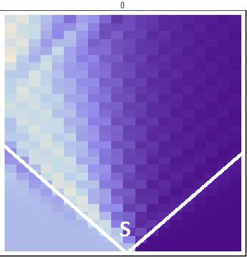
For a description of the probability density without approximations, see figure 3.

Many other examples of evolution can be studied in exact form by using several results on the closed summation of Bessel functions. In connection with diffraction problems by edges, we envisage a wide class of results by means of degenerate addition theorems where the summation index starts at $0$. Lommel expansions constitute another possibility. Take, for instance, an initial condition in the form of a ramp :

This poissonian profile represents the wave function of a particle that is trapped near the shutter, with a fastly decreasing tail. The function vanishes abruptly for negative positions and it can be regarded as a member of the family of edges. The real parameter $b$ determines the position of the maximum, e.g. for $b=1$ the maximum is exactly at the position of the edge. The evolution is obtained by computing the sum

where the second factor is manifestly regular at $t=0$. In this derivation we have used the Lommel expansion (formula (5) p. 141 [9])

From this result we can infer many properties that coincide with our previously obtained effects. For instance, using the first term in the ascending series of $J$ one can find constant probability curves involving $n$ and $t$, finding a short time behaviour of the caustics and a maximal velocity effect. A decreasing density in the form $1/t$ can be found from the asymptotic form of $J^{2}$. When $b=0$, we recover the point-like source.

For the sake of completeness, let us deal first with the two-dimensional continuous problem of a scalar plane wave scattered by an edge. The problem can be written in terms of forward and backward propagation (transmission and reflection) in the following manner: Suppose that a plane wave arrives at a screen positioned at $z=0$ and parallel to the $x$ axis (at this point, we make no further assumptions on the nature of such a physical obstacle). We have $\psi(z<0,x)=\exp(ik_{z}z+ik_{x}x)$ with $k_{z},k_{x}$ the corresponding components of the momentum. At $z=0$ we can impose an arbitrary boundary condition determined by the form of the screen; for definiteness we may put $\psi(0,x)=\theta(-x)e^{ixk_{x}}$. Set the energy $E=k_{x}^{2}+k_{z}^{2}$ such that

Since the solution of the problem satisfies the Helmholtz equation, it can be written formally as a continuous superposition of the form

where L and R indicate solutions propagating to the left and to the right, respectively. Now, let us assume no reflection ($A_{\rm{L}}=0,A_{\rm{R}}=1$)

and let us evaluate $\psi$ at $z=0$ in order to determine the distribution in $k$:

Substituting the inverse Fourier transform of the initial condition we have

Finally, the propagator in fictitious time $z$ and parameter $E$ is given by the factor in brackets

This integral can be evaluated upon a change of variables [21] and the appropriate choice of an integration contour. Let $\eta=E^{-1/2}(k+i\sqrt{E-k^{2}})$ and $\eta^{-1}=E^{-1/2}(k-i\sqrt{E-k^{2}})$, with an integration line given by the segments $\left\{\rm{Re}(\eta)<-1\right\}\cup\left\{\eta=e^{i\delta}|0<\delta<\pi\right\}\cup\left\{1>\rm{Re}(\eta)>0\right\}$. As there are no poles in the way, the upper semi-circular curve and the segment $(0,1)$ can be continuously deformed such that $\eta\in(-\infty,0)$. The integral in (51) is transformed to

The closed result is

where we have used the integral representation of the Hankel functions $H_{\pm 1}^{(1)}$ [13] and trivial algebraic manipulations. The result found here should not be confused with the usual Green’s function of the 2D Helmholtz equation subject to Sommerfeld’s outgoing radiation condition (given by the Hankel function $H_{0}^{(1)}$ alone). Our boundary condition has been defined along the $x$ axis at $z=0$.

It is important to note that in (53), the two limits $\sqrt{(x-x^{\prime})^{2}+z^{2}}\gg 1/\sqrt{E}$ (short wavelengths) and $(x-x^{\prime})^{2}/z^{2}\ll 1$ (paraxiality) must be taken simultaneously in order to recover the free Schrödinger propagator by means of the asymptotic form of the Hankel function:

The prefactor in brackets is related to the planewave propagating originally to the right on the left semi-plane $z<0$, with a wavelength $\lambda=2\pi/\sqrt{E}$.

Although the problem of diffraction by an edge has been discussed exhaustively in the literature, no description of the propagator (53) can be found in previous works. We should stress that this is the Euclidean version of a relativistic problem described by the Klein-Gordon equation [21]. Since the solutions to relativistic diffraction in time were identified as Lommel functions [7], we should expect similar results in our Euclidean case.

In connection with the validity of the approximations leading to the Schrödinger kernel, it is worth to mention that the problem of diffraction in propagation axis $z$ is characterized by infinitesimal oscillations near $z=0$ due to a dependence of the form $(x-x^{\prime})^{2}/z$ in (54). On the other hand, the kernel (53) exhibits a dependence on $\sqrt{(x-x^{\prime})+z^{2}}$ which is regular at $z=0$ and does not produce infinitesimal oscillations. Now that we have set the continuous example, we move to the discrete problem.

We turn our attention to the Helmholtz equation of one continuous variable $z$ and one discrete variable $n$. This problem also corresponds to a wave propagating in a 2D medium with one periodic direction (see section 5 and figure 5). The discrete derivative operator along the variable $n$ contains twice the identity operator, therefore it can be simplified by a redefinition of the energy in the full Helmholtz equation, leading to the analog of the l.h.s. of (2). We have

In complete analogy with the continuous 2D example, we state our boundary problem as follows: A Bloch wave propagates in the left semi-plane towards an absorptive edge, i.e. $\psi_{n}(z<0)=e^{ik_{x}n+ik_{z}z}$, where $k_{x}$ is Bloch’s quasi-momentum and $k_{z}$ is the momentum corresponding to coordinate $z$. The energy $E=k_{z}^{2}-2\cos k_{x}$ is fixed. The most general superposition which solves (55) when the wall is absorptive can be written as

where the integration over $k$ extends to the first Brillouin zone $(0,2\pi)$. The boundary condition at the position of the screen implies

References

- [1] Albert J P et al. 2002 Optical and Quantum Electronics 34 251-263.
- [2] Heeger A J et al. 1988 Rev Mod Phys 60 781–850.
- [3] Yablanovitch E 1987 Phys Rev Lett 58 2059-2062.
- [4] ’tHooft G 2012 Relating the quantum mechanics of discrete systems to standard canonical quantum mechanics. Preprint quant-ph/1204.4926v1.
- [5] ’tHooft G 2010 Int J Mod Phys 25 4385-4396.
- [6] Sadurní E, Seligman T H and Mortessagne F 2010 New J Phys 12 053014.
- [7] Moshinsky M 1952 Phys Rev 88 625-631.
- [8] Bloch F 1928 Z Phys 52 555-600.
- [9] Watson G N 1996 A Treatise on the Theory of Bessel Functions (Cambridge University Press, reprint 2nd edition).
- [10] Sadurní E 2012 Propagators in two-dimensional lattices. In preparation.
- [11] Dattoli G, Cesarano C and Migliorati M 2003 Int J Math 4 239-246.
- [12] Dattoli G, Migliorati M and Srivastava H M 2005 Journal of Computational and Applied Mathematics 173 149-154.
- [13] Gradshteyn I S and Ryzhik I M 2007 Table of Integrals, Series and Products (Academic Press, 7th edition).
- [14] Feynman R P and Hibbs A R 1965 Quantum Mechanics and Path Integrals (McGraw-Hill, New York).
- [15] Grosche C and Steiner F 1998 Handbook of Feynman Path Integrals (Springer).
- [16] Schulman L S 1996 Techniques and Applications of Path Integration (John Wiley and Sons).
- [17] There is a curious counterexample. Some relativistic propagators can be given as sums of paths in a “checker-board” model of space-time (p. 34 [14]). Such paths are continuous and their local velocity is equal in magnitude to . This discrete formulation does not apply to our non-relativistic framework.
- [18] Sadurní E 2012 J Phys: Conf Ser 343 012106.
- [19] Goldemberg J and Nussenzveig H M 1957 Rev Mex Fis VI.3 117-126.
- [20] NIST 2012 Handbook of Mathematical Functions, Chapter 10.20. Online at http://dlmf.nist.gov/10.20
- [21] Moshinsky M and Sadurní E 2008 Rev Mex Fis S 54 (3) 92-98.
- [22] It is possible to construct an expansion of the propagator in terms of associated Legendre functions of variable by using Bessel operators acting on (the symbolic form of Gegenbauer equation, p.140 in [9]). Another expansion of fast convergence can be obtained by noting that is the generator of Bessel polynomials of variable and parameter .