De Sitter Musings

The pure four-dimensional de Sitter geometry is a maximally symmetric solution to Einstein’s equations:

$$\mathcal{G}_{\mu\nu}\equiv R_{\mu\nu}-\frac{1}{2}g_{\mu\nu}R+\Lambda g_{\mu\nu}=0\penalty\ ,$$

(1.1)

with $\Lambda\equiv+3/\ell^{2}$ a positive cosmological constant. The cosmological constant measured in our own universe is given by $\Lambda\sim 10^{-52}\;\text{m}^{-2}$. The de Sitter geometry can be viewed as the induced metric on the four-dimensional hyperboloid:

$$-X_{0}^{2}+\sum_{i=1}^{4}X_{i}^{2}=\ell^{2}\penalty\ ,$$

(1.2)

embedded in five-dimensional Minkowski space: $ds^{2}=-dX_{0}^{2}+dX_{i}^{2}$. The various coordinate patches of de Sitter space cover some or even all of the hyperboloid. In what follows, we will restrict our discussion to four dimensions unless otherwise specified.

The global geometry is described by the metric:

$$ds^{2}=-d\tau^{2}+\ell^{2}\cosh^{2}\frac{\tau}{\ell}\left(d\psi^{2}+\sin^{2}\psi d\Omega^{2}_{2}\right)\penalty\ ,$$

(1.3)

where $\tau\in\mathbb{R}$ and $d\Omega^{2}_{2}\equiv d\theta^{2}+\sin^{2}\theta d\phi^{2}$ being the round metric on the unit two-sphere. Constant $\tau$ surfaces are three-spheres which shrink from $\mathcal{I}^{-}$ at $\tau=-\infty$ to $\tau=0$ and grow from $\tau=0$ to $\mathcal{I}^{+}$ at $\tau=+\infty$. The Penrose diagram of global de Sitter is depicted by a square as seen in figure 1.1. Sometimes, it is more convenient to describe one half of the global geometry using planar spacelike slices:

$$ds^{2}=-dT^{2}+\ell^{2}e^{2T/\ell}d\vec{x}^{2}=\frac{\ell^{2}}{\eta^{2}}\left(-d\eta^{2}+d\vec{x}^{2}\right)\penalty\ ,$$

(1.4)

with $\vec{x}\in\mathbb{R}^{3}$ and $T\in\mathbb{R}$. This coordinate patch is depicted in figure 1.2. The coordinate $\eta=-e^{-T/\ell}$ is known as the conformal time coordinate. The planar metric covers the region of space inside and including the lightcone emanating from a single point at $\mathcal{I}^{-}$ (which lives at $T\to-\infty$). One can similarly describe the region of space inside and including the past lightcone emanating from a point at $\mathcal{I}^{+}$ with the same coordinate system. In this case it is convenient to take $T\to-T$ and $\eta\to-\eta$ to keep the time coordinates increasing in the forward time direction.

Neither the global nor the planar geometries can be completely accessed by a single observer. Instead, the region of space accessible to a single observer is known as the the static patch and described by the metric:

$$ds^{2}=-\left(1-\frac{r^{2}}{\ell^{2}}\right)dt^{2}+\left(1-\frac{r^{2}}{\ell^{2}}\right)^{-1}{dr^{2}}+r^{2}d\Omega^{2}_{2}\penalty\ .$$

(1.5)

The coordinate ranges are $r\in[0,\ell]$ and $t\in\mathbb{R}$. One may notice that the norm of the $\partial_{t}$ Killing vector vanishes at $r=\ell$. Indeed, $r=\ell$ is a null surface that surrounds the observer at all times, known as the cosmological horizon. One can also describe the region to the future the cosmological horizon $r\in(\ell,\infty)$ with the above coordinate system, and it describes what is known as the future triangle. A similar statement is true for the region to the past of the cosmological horizon. We can also consider an extension of the static patch that includes the region in a single static patch as well as the future triangle which is smooth across the horizon:

$$\frac{ds^{2}}{\ell^{2}}=\left(-\frac{\rho}{\alpha}+\rho^{2}\right)d\tau^{2}+d\tau d\rho+\left(1-2{\alpha}{\rho}\right)^{2}d\Omega_{2}^{2}\penalty\ ,$$

(1.6)

with $\tau\in\mathbb{R}$ and $\rho\in(1/2\alpha,-\infty)$ with $\mathcal{I}^{+}$ at $\rho\to-\infty$. Constant $\rho$ slices are null rays emanating from the worldline at $\rho=1/2\alpha$ reaching all the way out to $\mathcal{I}^{+}$. The horizon is at $\rho=0$. The patches (1.5) and (1.6) are depicted in figure 1.1.

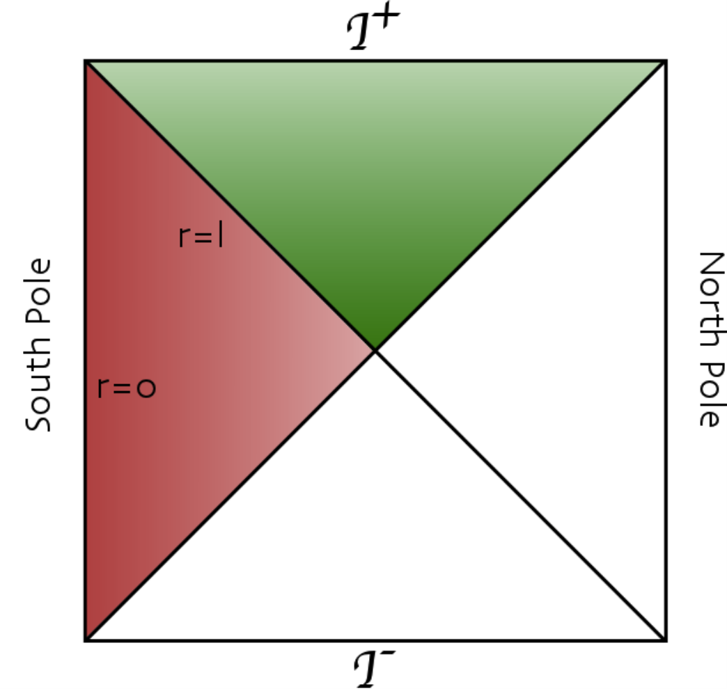
We can also describe the hyperbolic patch of de Sitter space described by the metric:

$$ds^{2}=-d\tilde{t}^{2}+\ell^{2}\sinh^{2}\frac{\tilde{t}}{\ell}\;d\mathcal{H}^{2}_{3}\penalty\ ,$$

(1.7)

where $\tilde{t}\in\mathbb{R}$ and $d\mathcal{H}_{3}^{2}=dR^{2}+\sinh^{2}Rd\Omega_{2}^{2}$ is the standard metric of hyperbolic three-space.¹¹ 1 It is worth mentioning that this geometry (with negative curvature constant $\tilde{t}$ spacelike slices) is the geometry that arises inside a positive $\Lambda$ Coleman-De Luccia bubble nucleated in some false vacuum. Another patch of de Sitter space is radially foliated by three-dimensional de Sitter space and we call it the de Sitter/de Sitter patch:

$$ds^{2}=dw^{2}+\sin^{2}\frac{w}{\ell}\left(-d\tilde{\tau}^{2}+\ell^{2}\cosh^{2}\frac{\tilde{\tau}}{\ell}d\Omega^{2}_{2}\right)\penalty\ .$$

(1.8)

The coordinate regions are now $w\in[0,\pi]$ and $\tilde{\tau}\in\mathbb{R}$. Notice that there is a horizon at $w=0$ and $w=\pi$. The de Sitter/de Sitter and hyperbolic patches are depicted in figure 1.2. Finally, we can have a patch foliated by $\mathcal{H}_{2}\times\mathbb{R}$ slices:

$$ds^{2}=-\frac{d\tau^{2}}{\left(1+(\tau/\ell)^{2}\right)}+\left(1+(\tau/\ell)^{2}\right)dx^{2}+\tau^{2}d\mathcal{H}_{2}^{2}\penalty\ ,$$

(1.9)

with $\tau\in\mathbb{R}$, $x\sim x+\ell$ and $d\mathcal{H}_{2}^{2}=dR^{2}+\sinh^{2}Rd\phi^{2}$ is the standard metric on hyperbolic two-space.

The isometries of four-dimensional de Sitter space are given by $SO(4,1)$. This isometry group manifests itself as the conformal group of the three-metric on $\mathcal{I}^{\pm}$ which may be $\mathbb{R}^{3}$, $S^{2}\times\mathbb{R}$, $\mathcal{H}_{3}$, $\mathcal{H}_{2}\times{S^{1}}$ or $S^{3}$ in the case of pure de Sitter. There is no global timelike Killing vector and hence no positive energy theorem, at least in its traditional form. In fact, global slices are compact and consequently conserved (gauge) charges vanish on global slices. One may also consider solutions given by smoothly quotienting the metric on $\mathcal{I}^{+}$. For example we can quotient $\mathbb{R}^{3}$ to a three-torus and $\mathcal{H}_{3}$ to a compact hyperbolic three-manifold. In doing so, one may develop singularities in the bulk where cycles shrink to zero size.

As a final note on the geometry of pure de Sitter space, we mention that its Euclideanization is given by the round metric on the four-sphere. In global coordinates this can be seen by taking $\tau\to i\tau$, in static patch coordinates by taking $t\to it$, in de Sitter/de Sitter coordinates by taking $\tilde{\tau}\to i\tilde{\tau}$ and in hyperbolic coordinates by taking $d\mathcal{H}_{3}^{2}\to-d\Omega_{3}^{2}$ and $\tilde{t}\to i\tilde{t}$.

Perhaps the basic unresolved question for asymptotically de Sitter universes regards the (non)-existence of precise observables (see for example [9, 10]). In a theory of gravity we must let go of our notions of local observables, as attempting to collect too much information in a confined region of space will eventually cause a gravitational backreaction, and in the most dramatic of cases lead to the formation of a black hole. To avoid this, we typically consider data living at some asymptotic region of space. For example, we could consider the the S-matrix at null infinity of asymptotically flat space or the boundary correlators at the timelike boundary of asymptotically anti-de Sitter spacetimes. De Sitter space has no such asymptotic region given that observers are surrounded by a finite size cosmological horizon. Instead it has asymptotic regions in the infinite future and past. These are infinite spacelike slices which are causally inaccessible to a single observer, save a horizon sized region. Thus, there is a classical uncertainty associated with the measurements of asymptotically de Sitter observers. On the other hand, if the de Sitter length is parametrically large compared to the Planck scale, we should be able to make increasingly precise observations. These observations are naturally made as the data reaches the worldtube of an observatory inside the cosmological horizon.

In this spirit, we begin our discussion with a classical consideration of asymptotically de Sitter universes and the different notions of data used to specify the initial value problem.

Ordinarily, the way we think about classical gravity is to impose some data, subject to constraints, on a spacelike slice $\Sigma_{0}$ and evolve it to the future using Einstein’s equations $\mathcal{G}_{\mu\nu}$. This is known as the Cauchy problem in general relativity [11, 12, 13]. The data is given by the induced metric on $\Sigma_{0}$, denoted by $h_{\mu\nu}$, and the extrinsic curvature of the Cauchy foliation $k_{\mu\nu}$. Let the timelike unit normal to $\Sigma_{0}$ be given by $n^{\mu}$, such that $h_{\mu\nu}=g_{\mu\nu}+n_{\mu}n_{\nu}$ and $k_{\mu\nu}=\mathcal{L}_{n}h_{\mu\nu}/2$. One finds that the equations $n_{\mu}n_{\nu}\mathcal{G}^{\mu\nu}=n_{\mu}\mathcal{G}^{\mu i}=0$ (the index $i$ is tangent to $\Sigma_{0}$) contain only first derivatives in time and thus act as constraints on $h_{\mu\nu}$ and $k_{\mu\nu}$. These are the momentum and Hamiltonian constraints related to coordinate reparameterizations on $\Sigma_{0}$ and the absence of a local notion of energy in general relativity due time reparameterization invariance. Evolving the constrained data from $\Sigma_{0}$ determines the solution in the domain of dependence $\mathcal{D}(\Sigma_{0})$ of $\Sigma_{0}$, given by all points whose causal past lies on $\Sigma_{0}$ (see figure 2.1). We can apply the Cauchy problem to Einstein gravity in the presence of a cosmological constant $\Lambda\equiv+3/\ell^{2}$. Given that the global spacelike slices are compact, data on an initial spacelike slice $\Sigma_{0}$ determines the geometry all the way into the future. This may evolve toward a singular solution or to a smooth $\mathcal{I}^{+}$ depending on the initial data.

A large class of late time nonlinear solutions²² 2 Though we do not discuss linearized gravity in a fixed de Sitter background in this article, a very complete discussion can be found in [14, 15]. can be expressed as a Fefferman-Graham expansion [16, 17] in a small parameter $\eta$:

$$\frac{ds^{2}}{\ell^{2}}=-\frac{d\eta^{2}}{\eta^{2}}+\frac{1}{\eta^{2}}\left(g^{(0)}_{ij}+\eta^{2}g^{(2)}_{ij}+\eta^{3}g^{(3)}_{ij}+\ldots\right)dx^{i}dx^{j}\penalty\ .$$

(2.1)

The coordinate $\eta$ is the conformal time and the limit $\eta\to 0$ is a late time spacelike slice that tends to $\mathcal{I}^{+}$. We have fixed the synchronous gauge $g_{\eta\eta}=-\eta^{-2}$ and $g_{\eta i}=0$. The boundary data is given by the three-metric $g^{(0)}_{ij}$ on $\mathcal{I}^{+}$ and a transverse-traceless tensor $g^{(3)}_{ij}$, $\text{tr}_{g^{(0)}}g^{(3)}_{ij}=\nabla^{i}_{g^{(0)}}g^{(3)}_{ij}=0$. The coefficients of all other powers of $\eta$ are completely determined by $g^{(0)}$ and $g^{(3)}$.³³ 3 For example $g^{(2)}_{ij}=R_{ij}[g^{(0)}]-R[g^{(0)}]g^{(0)}_{ij}/4$, which is the Schouten tensor of $g^{(0)}_{ij}$ in three-dimensions. One can use diffeomorphisms tangent to $\mathcal{I}^{+}$ to kill three components of $g^{(0)}_{ij}$ and one of the four-dimensional ones to fix its determinant, leaving two degrees of freedom in $g^{(0)}_{ij}$. The transverse-traceless property of $g^{(3)}_{ij}$ leaves two degrees of freedom in $g^{(3)}_{ij}$ as well. Together, $\left(g^{(0)}_{ij},g^{(3)}_{ij}\right)$ form the boundary data of an asymptotically de Sitter universe. More precisely, it is the conformal class $\left(g^{(0)}_{ij},g^{(3)}_{ij}\right)\sim\left(\Omega^{2}g^{(0)}_{ij},\Omega^{-1}g^{(3)}_{ij}\right)$, for some smooth non-zero function $\Omega(x^{i})$, that constitutes the boundary data.

An important mathematical theorem due to Friedrich [18], is that the above Cauchy problem is well posed. Given the data $\left(g^{(0)}_{ij},g^{(3)}_{ij}\right)$ at $\mathcal{I}^{+}$ and assuming the Cauchy slices are compact (though not necessarily topologically three-spheres) there is a unique extension of the solution into the bulk realizing the data at $\mathcal{I}^{+}$. Furthermore, small deviations from this data result in small variations of the extended bulk solution. The result was extended to all even dimensions by Anderson [19]. From the other end, one can ask what class of initial conditions leads to an asymptotically (locally) de Sitter universe in the future. It has been proposed in what has come to be known as the cosmic no hair theorem [6, 20] that (almost) all expanding solutions of the Einstein equations in the presence of a positive $\Lambda$ classically evolve to a locally de Sitter universe in the far future. This proposal has been verified for several classes of geometries [21, 22, 23, 24], though a small class of counterexamples is also known.

A large class of $\left(g^{(0)}_{ij},g^{(3)}_{ij}\right)$ at $\mathcal{I}^{+}$ will contain a big bang type singularity in the past. Similarly, given that the global geometry is contracting if we begin at $\mathcal{I}^{-}$, a large class of data at $\mathcal{I}^{-}$ will never evolve into asymptotically de Sitter space due to the formation of a big crunch. There exist results of interest relating the topology and curvature of the geometry at $\mathcal{I}^{\pm}$ with the existence of bulk singularities [25]. For instance, in four dimensions in order for there to be a geometry smoothly connecting $\mathcal{I}^{-}$ to $\mathcal{I}^{+}$ the (compact) Cauchy surfaces must have a finite fundamental group, like $S^{3}$ or quotients thereof. Also, if the conformal class of metrics on $\mathcal{I}^{-}$ contains a metric with constant negative scalar curvature then all timelike geodesics are future incomplete [25].

Recall that the global geometry of asymptotically de Sitter spacetimes cannot be completely accessed by a local observer. From a local perspective, such as an observer restricted to a lab confined to live inside some finite size worldtube, a large part of the initial data on the $\Sigma_{0}$ will remain out of causal contact and never be observed.⁴⁴ 4 We are assuming here that there is no exit from inflation, i.e. our space is asymptotically de Sitter everywhere. Observers that do exit from inflation may be able to access a larger part of $\Sigma_{0}$. We can picture this by drawing the past null cone of the lab wall which has reached $\mathcal{I}^{+}$. In particular, we can partition $\Sigma_{0}$ into its observable part $\Sigma_{obs}$ and its unobservable part $\Sigma_{u}$. The physical relevance of data that is forever unobservable is questionable. In any event, we are prompted to consider a more ‘observer friendly’ boundary value problem. This was addressed for vanishing $\Lambda$ by Tamburino and Winicour [26]. These authors considered the problem of data on a worldtube $\Gamma$ of some finite thickness and a null surface $N_{0}$ emanating toward the future from some initial spacelike slice of $\Gamma$ which we may denote by $S_{0}$ (see figure 2.1). A natural coordinate system for this problem, first considered in [27, 28], is:

$$ds^{2}=-g_{uu}du^{2}-2\left(g_{ur}dr+g_{ua}dx^{a}\right)du+r^{2}\bar{g}_{ab}dx^{a}dx^{b}\penalty\ ,\quad a,b=1,2\penalty\ .$$

(2.2)

The determinant of $\bar{g}_{ab}$ is fixed to be: $\det\bar{g}_{ab}=f(x^{a})^{2}$ where $f(x^{a})$ is a function of the $x^{a}$ only. The $u$-coordinate is a timelike coordinate on the worldline and the $r$-coordinate describes the position on the null surface emanating from $\Gamma$ at some given $u$. The $x^{a}$-coordinates describe the position on the two-sphere at constant $r$ and $u$.

It was shown [26] (see also [29]) that knowing $\bar{g}_{ab}$ on $\Gamma$ as a function of $u$ and $x^{a}$, $\bar{g}_{ab}$ on $N_{0}$ as a function of $r$ and $x^{a}$ and $g_{uu}$, $g_{ua,r}$ on $S_{0}$ (as functions of $x^{a}$ only) allows us to determine the solution to Einstein’s equation in the region between $\Gamma$ and $N_{0}$. Though this problem has not been addressed in the context of Einstein’s equations with positive $\Lambda$ and it would be very interesting to do so. In particular, one might want to understand the relation between the data on $\left(\Gamma,N_{0},S_{0}\right)$ and the Fefferman-Graham data $\left(g^{(0)}_{ij},g^{(3)}_{ij}\right)$ at $\mathcal{I^{+}}$. It is also worth mentioning that the consideration of data on a timelike surface has played a role in asymptotically anti-de Sitter spacetimes. In this case, one specifies sources on the timelike boundary and studies their response by solving for the bulk.

For the sake of completeness we mention two other boundary value problems that have been considered when studying Einstein’s equations with vanishing cosmological constant. These are depicted in figure 2.2.

The first is the Bondi problem [27], which was considered in [30] for four dimensional de Sitter space. The worldline data on $\Gamma$ we previously considered is pushed all the way to $\mathcal{I}^{+}$. This data, which lives on an interval of $\mathcal{I}^{+}$, in addition to the data on a null slice $N_{0}$ emanating from a localized radiating source to $\mathcal{I}^{+}$ as well as data on a two-sphere $S^{0}$ at $\mathcal{I}^{+}$ specifies a solution.

The other setup, considered by Sachs [31], specifies data on two null slices intersecting at a common two-surface $\Sigma$. For the double null problem (with $\Lambda=0$), one builds a line element of the form:

$$ds^{2}=-e^{2q}dudv+e^{2h}\bar{g}_{ab}\left(dx^{a}+C^{a}du\right)(dx^{b}+C^{b}du)\penalty\ ,$$

(2.3)

with $\det{\bar{g}_{ab}}=1$, $C^{a}=0$ on the initial null slice $v=v_{0}$ and $q=0$ on the initial null slices $v=v_{0}$, $u=u_{0}$. The data $\bar{g}_{ab}(x^{a},u)$ on $v=v_{0}$ and $\bar{g}_{ab}(x^{a},v)$ on $u=u_{0}$ in addition to $h$, $C_{a,v}$, $h_{,u}$ and $h_{,v}$ on $\Sigma$ determine a solution to the future of the null slices. It can be shown that an analogous setup exists in the presence of a non-vanishing, positive $\Lambda$ [32]. We should emphasize that constructing the geometry in the future triangle (outside the observer’s horizon) from data on two null slices allows us to keep track of how this geometry is related to the data of the Northern and Southern static patches in figure 1.1. For instance, it allows is to consider variations of the data from a single static patch on the $v=v_{0}$ null slice while maintaining the data on the $u=u_{0}$ null slice fixed.

The notion of symmetry in theories of gravity is subtle. Though some special solutions have an isometry group associated to them, generically this is not the case since the metric is sensitive to all surrounding matter and the symmetries are destroyed. A useful notion that appears in the context of classical general relativity is that of asymptotic symmetries. These are the set of diffeomorphisms $\xi^{\mu}$, subject to some (physically motivated) boundary condition, that alter the physical boundary data. In certain circumstances, one can associate to each of the asymptotic symmetries a charge $Q_{\xi}$ generating the symmetry and study the algebra of the charges. Choosing the appropriate boundary condition is somewhat context dependent. A well known example is given by the symmetry group of asymptotically flat spacetimes. This was defined in the seminal works of Bondi, Metzner [27] and Sachs [33]. They found that the asymptotic symmetries of asymptotically flat spaces comprise an infinite dimensional group, the BMS group, containing the (finite dimensional) Poincare symmetry as a subgroup.

The asymptotic symmetry group of four-dimensional de Sitter space has been analogously studied [30, 34, 35, 36]. In the global case it was found that for boundary conditions allowing variations of the conformal metric $g^{(0)}_{ij}$ on $\mathcal{I}^{+}$ the asymptotic symmetries comprise the full set of diffeomorphisms tangent to $\mathcal{I}^{+}$. Given a bulk spacelike three-slice $\Sigma$ intersecting $\mathcal{I}^{+}$ at some two-slice $\partial\Sigma$, the charges associated to the $\xi$ are found to be⁵⁵ 5 Notice that the charges are given solely by a boundary term which would not be present if the slice did not cut $\mathcal{I}^{+}$ at some $\partial\Sigma$. Indeed on a compact global three-slice $\Sigma$ the charges above would vanish. the Brown-York charges [37, 38, 39, 40, 41, 42, 43]

$$Q_{\xi}[\partial\Sigma]=-\frac{3\ell}{16\pi G}\int_{\partial\Sigma}d^{2}x\sqrt{\sigma}n^{i}\xi^{j}g^{(3)}_{ij}\penalty\ ,$$

(2.4)

where $\sigma$ is the determinant of the induced metric on $\partial\Sigma$ and $n^{i}$ is normal to $\partial\Sigma$. Furthermore, the flux between bulk two slices intersecting $\mathcal{I}^{+}$ at $\partial\Sigma_{1}$ and $\partial\Sigma_{2}$ is given by [34]:

$$Q_{\xi}[\partial\Sigma_{2}]-Q_{\xi}[\partial\Sigma_{1}]=-\frac{3\ell}{32\pi G}\int_{\mathcal{B}_{12}}g^{(3)ij}\mathcal{L}_{\xi}{g^{(0)}_{ij}}\sqrt{g^{(0)}}d^{3}x\penalty\ .$$

(2.5)

where $\mathcal{B}_{12}$ is the region on $\mathcal{I}^{+}$ between $\partial\Sigma_{1}$ and $\partial\Sigma_{2}$.

As we mentioned before, for a local (eternally de Sitter) observer who cannot access the full data on a spacelike slice $\Sigma_{0}$, it is unclear what the physical meaning of the inaccessible data is. On the other hand, along with the wordline data of the observer herself, this inaccessible data determines the geometry outside the cosmological horizon, i.e. in the future triangle. Thus, one may ponder on other interesting ways to fix the data on $\Sigma_{u}$. One motivation may come from requiring that the asymptotic symmetries comprise the isometry group of pure de Sitter space, $SO(4,1)$, in analogy to the case of anti-de Sitter space. In order to do so, one could tune the data on $\Sigma_{u}$ such that for any variation of data on $\Gamma$ and the observable part of $N_{0}$, the variations of $g^{(0)}_{ij}$ vanish. Though such an initial value problem severely violates causality, this violation is classically inaccessible to the local observer. Evidence that this is possible was given at the linearized level in [35]. Another possibility is to consider freezing the unobservable data, such that the variations of data reaching $\mathcal{I}^{+}$ are encoded fully by variations of data on $\Gamma$ and the observable part of $N_{0}$ [44].

Let us now consider again the local observer and her worldtube. If we push the size of our worldtube to approach the de Sitter radius $\ell$, we are forced to study the dynamics of metric deformations very near the cosmological horizon. The problem mimics similar analyses in the context of the near horizon regions of black hole geometries [45, 46, 47, 48, 49, 50] beginning with the seminal work of Damour [51]. The basic idea is that solutions to Einstein’s equations in the near horizon limit are organized in the form of solutions to a Navier-Stokes equation. This is related to the fact that near horizon regions encode the deep infrared behavior of fields (due to an increasing redshift factor) and the Navier-Stokes equation encodes the deep infrared physics of a rather universal set of systems. It was shown in [44] that the dynamics of non-linear metric deformations very near the cosmological horizon are indeed governed by the incompressible (non-relativistic) Navier-Stokes equation. The radial direction emanating away from the timelike surface is $\rho$ and the time coordinate is $\tau$. Constant $\tau$ and $\rho$ surfaces are two-spheres parametrized by $\Omega=(\theta,\phi)$. The deformation is expanded in a dimensionless near horizon parameter $\alpha$ which is taken to be small, and parametrized by $v^{i}$, $P$ and $\phi_{i}^{\left(\alpha\right)}$ which are functions of $(\tau,\Omega^{i})$ only. As Dirichlet boundary conditions on the $\rho=1$ timelike hypersurface (which in the $\alpha\to 0$ limit is parametrically close to the horizon) one requires the perturbations to preserve the induced metric on the hypersurface $\rho=1$:

$$ds_{3d}^{2}=\left(-\frac{1}{\alpha}+1\right)d\tau^{2}+\left(1-2\alpha\right)^{2}d\Omega^{2}_{2}\penalty\ ,$$

(2.6)

up to a conformal factor:

$$1+2\alpha P+\mathcal{O}(\alpha^{2})\penalty\ .$$

(2.7)

Then, imposing the Einstein equations with $\Lambda>0$ and taking the limit $\alpha\to 0$, $v^{i}$ and $P$ are found to obey:

$$\partial_{\tau}v^{i}+\nabla_{S^{2}}^{i}P+v_{j}\nabla^{j}_{S^{2}}v^{i}-\nu\left(\nabla^{2}_{S^{2}}v^{i}+R^{i}_{j}v^{j}\right)=0\penalty\ ,\quad\nabla_{S^{2}}^{i}v_{i}=0\penalty\ ,$$

(2.8)

to leading order in $\alpha$. As mentioned, this is nothing more than the incompressible Navier-Stokes equation with $\nu=1+\mathcal{O}(\alpha)$.

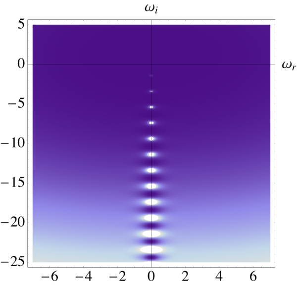
As a final note we discuss the quasinormal mode spectrum of de Sitter space. Quasinormal modes are a particular set of perturbative modes that encode the dissipative nature or ‘ringing’ of a given background [52]. The recipe to compute them is given by solving the linearized equations of motion of some matter field, such as the graviton, and demanding that the solutions obey specific properties. In the case of an asymptotically flat Schwarzschild solution, it is demanded that the modes are purely outgoing at future null infinity and purely infalling into the black hole’s future horizon. In the de Sitter case [53], working with the static patch coordinates (1.5), we impose no incoming flux from the past cosmological horizon and that the modes be regular near the worldline at $r=0$. The idea is to capture the ringing of the spacetime by sending an isolated pulse from the worldline and study the behavior at late times.

As an example consider a scalar field $\Phi(x)$ of mass $m$. Expanding the field in a Fourier basis $\Phi(x)=e^{-i\omega t}Y_{lm}(\theta,\phi)R_{lm}^{\omega}(r)$, we find that these boundary conditions restrict the $\omega$’s to a discrete set:

$$\omega^{\pm}_{n}\ell=-i\left(2n+l+\frac{3}{2}\pm\sqrt{\frac{9}{4}-m^{2}\ell^{2}}\right)\penalty\ .$$

(2.9)

Similar results hold for more general fields. Notice that for sufficiently light fields, the de Sitter quasinormal mode spectrum is pure imaginary. This is in contrast to the quasinormal mode spectrum of the Schwarszchild black hole [54, 55, 56] or asymptotically AdS black holes [57, 58] which typically have a real part which is some function of the momenta. Given that $\omega_{n}^{\pm}$ have a negative imaginary part, the de Sitter quasinormal modes decay exponentially at late times.

In the case $r_{c}\to r_{+}$ we can in fact take a near horizon limit, zooming into the region between the horizons. This is accomplished by introducing:

$$\tau=\lambda t/r_{c}\penalty\ ,\quad\rho=\frac{r-r_{+}}{r_{c}\lambda}\penalty\ ,\quad\beta=\frac{r_{c}-r_{+}}{r_{c}\lambda}\penalty\ ,$$

(3.3)

and taking the limit $\lambda\to 0$ while keeping $\beta$ fixed. This leads to the Nariai metric [62]:

$${ds^{2}}=\frac{\ell^{2}}{3}\left(-d\tau^{2}\rho(\rho-\beta)+\frac{d\rho^{2}}{\rho(\rho-\beta)}+d\Omega^{2}_{2}\right)\penalty\ ,$$

(3.4)

which is nothing more than the dS${}_{2}\times S^{2}$ geometry. The Penrose diagram of dS₂ is depicted in figure 3.2. The original black hole horizon now lives at $\rho=0$ and the cosmological horizon lives at $\rho=\beta$. The quasinormal modes of the Nariai black hole in de Sitter space were considered in [65] and are found to be:

$$\omega_{n}\ell=\frac{\beta}{6}\left(-\left(n+\frac{1}{2}\right)i+\sqrt{(l+2)(l-1)-\frac{1}{4}}\right)\penalty\ ,$$

(3.5)

where $l$ is the angular momentum on the $S^{2}$ and the frequency $\omega_{n}$ is measured with respect to the $\tau$-coordinate in (3.4). When geodesically completing the space to:

$$ds^{2}=\frac{1}{3}\left(-d\tau^{2}+\cosh^{2}\frac{\tau}{\ell}d\psi^{2}+\ell^{2}d\Omega_{2}^{2}\right)\penalty\ ,$$

(3.6)

a new future/past boundary $\mathcal{I}^{\pm}_{N}$ develops at $\tau\to\pm\infty$. Notice that (3.6) is not an asymptotically dS₄ universe. On the other hand, it is unknown what class of initial Cauchy data preserves the asymptotic structure of the global Nariai universe and it may be extremely limited [63, 64].

Had we also included angular momentum we would have found a similar near horizon limit whose geometry is given by the one-parameter family of rotating Nariai metrics. In global coordinates:

$$ds^{2}=\Gamma(\theta)\left[-d\tau^{2}+\cosh^{2}\frac{\tau}{\ell}d\psi^{2}+\alpha(\theta)d\theta^{2}\right]+\gamma(\theta)\left(d\phi-k\sinh\frac{\tau}{\ell}d\psi\right)^{2}\penalty\ .$$

(3.7)

The functions $\Gamma(\theta)$, $\alpha(\theta)$ and $\gamma(\theta)$ can be found in [66, 67]. Geometrically, the space is an $S^{2}$ fibered over a dS₂ base space and there exists a future and past boundary $\mathcal{I}^{\pm}_{RN}$ at $\tau\to\pm\infty$. In this limit, $a$ and $M$ are related to $r_{c}$ as:

$$a^{2}=\frac{r_{c}^{2}\left(1-3r_{c}^{2}/\ell^{2}\right)}{1+r_{c}^{2}/\ell^{2}}\penalty\ ,\quad M=\frac{r_{c}\left(1-r^{2}_{c}/\ell^{2}\right)^{2}}{1+r_{c}^{2}/\ell^{2}}\penalty\ .$$

(3.8)

It is worth mentioning that the asymptotic symmetry group at $\mathcal{I}^{+}_{RN}$ of the rotating Nariai geometry is the (infinite-dimensional) Virasoro algebra with central charge [67]:

$$c_{L}=\frac{12r_{c}^{2}\sqrt{\left(1-3r_{c}^{2}/\ell^{2}\right)\left(1+r_{c}^{2}/\ell^{2}\right)}}{-1+6r_{c}^{2}/\ell^{2}+3r_{c}^{4}/\ell^{4}}\penalty\ .$$

(3.9)

The Virasoro algebra is the symmetry group of two-dimensional conformal field theories and may suggest that the language of 2d CFT’s is intricately connected to the rotating Nariai geometry, perhaps holographically. Further evidence for this idea was pursued through an extensive study of quantum fields in the rotating Nariai background [68]. We could also consider adding a $U(1)$ gauge symmetry and study charged black holes in de Sitter space. Quite remarkably, in this case a set of time dependent multi-black hole solutions have been discovered by Kastor and Traschen [69].

Finally, we would like to make a brief comment about a set of black hole solutions to Einstein gravity with a negative cosmological constant, known as topological AdS₄ black holes. These black holes have a horizon with a $\mathcal{H}_{2}$ geometry and can have lower energy than the AdS₄ vacuum with $\mathcal{H}_{2}$ slicing. However, their energy is bounded from below by the critical hyperbolic black hole which has a near horizon geometry given by AdS${}_{2}\times\mathcal{H}^{2}$. The set of topological AdS₄ black holes with energy lower than the AdS₄ vacuum is a direct analytic continuation of the de Sitter black holes and in particular, the AdS${}_{2}\times\mathcal{H}_{2}$ solution is an analytic continuation of the dS${}_{2}\times S^{2}$ Nariai solution.

Let us for simplicity consider a free scalar field $\Phi(x)=\eta\varphi(\eta)e^{i\vec{k}\cdot\vec{x}}$ with mass $m$ in a fixed de Sitter background with planar slices (1.4). The wave equation is given by:

$$\left(\eta^{2}\partial_{\eta}\eta^{-2}\partial_{\eta}+k^{2}\right)\eta\varphi=-\eta^{-1}\ell^{2}m^{2}\varphi\penalty\ .$$

(4.1)

There are two-linearly independent solutions to this equation given by:

$$\varphi_{1}=\frac{1}{2}(\pi\eta)^{1/2}J_{\nu}(k\eta)\penalty\ ,\quad\varphi_{2}=\frac{1}{2}(\pi\eta)^{1/2}Y_{\nu}(k\eta)\penalty\ .$$

(4.2)

We have normalized with respect to the Klein-Gordon inner product,

$$(\varphi_{n},\varphi_{m})=-i\int_{\Sigma}d^{3}x\sqrt{h}n^{\mu}\left(\eta\varphi_{n}\overleftrightarrow{\partial_{\mu}}(\eta\varphi_{m}^{*})\right)=\delta_{nm}\penalty\ ,$$

(4.3)

where $\Sigma$ is a spacelike three-slice with induced metric $h_{ij}$ and future directed norm $n^{\mu}$. The functions $J_{\nu}(z)$ and $Y_{\nu}(z)$ are Bessel functions of the first and second kind and $\nu\equiv\sqrt{9/4-m^{2}\ell^{2}}$. One can also solve the equation of motion near $\mathcal{I}^{+}$, i.e. $\eta\to 0$, to find the following asymptotic form:

$$\varphi_{\pm}\sim(-\eta)^{1/2\pm\nu}\penalty\ .$$

(4.4)

Notice that $\varphi_{+}$ becomes an oscillatory mode with positive frequency $|\nu|$ for $m\ell>3/2$. Finally, we can examine the modes in the region $k|\eta|\to\infty$ residing well within the cosmological horizon. We find that the combination:

$$\lim_{k\eta\to\infty}\left(\varphi_{1}-i\varphi_{2}\right)\to\frac{1}{\sqrt{2k}}e^{-ik\eta}\penalty\ ,$$

(4.5)

is equivalent to a positive frequency mode in Minkowski space with respect to the canonical vacuum state.

Positive frequency modes in the Bunch-Davies (or Euclidean) vacuum state $|E\rangle$ are those which become the positive frequency modes in Minkowski space upon taking the limit $k|\eta|\to\infty$ [71] (see also [72]). These are given precisely by $\varphi_{E}\equiv\varphi_{1}-i\varphi_{2}$. We can thus expand our quantum field in terms of the creation and annihilation operators of $|E\rangle$:

$$\hat{\varphi}_{E}(\eta,\vec{x})=\sum_{k>0}\left[a_{k}^{E}\varphi_{E,k}(\eta)e^{i\vec{k}\cdot\vec{x}}+(a^{E}_{k})^{\dagger}\varphi_{E,k}^{*}(\eta)e^{-i\vec{k}\cdot\vec{x}}\right]\penalty\ .$$

(4.6)

The creation and annihilation operators satisfy the usual properties:

$$a_{k}^{E}|E\rangle=0\penalty\ ,\quad[a_{k}^{E},(a^{E}_{k^{\prime}})^{\dagger}]=\delta_{kk^{\prime}}\penalty\ .$$

(4.7)

As usual we can build a host of other states by acting with $a_{k}^{E}$ and $(a^{E}_{k})^{\dagger}$ on $|E\rangle$. We will discuss several features of $|E\rangle$ in the following subsections.

One need not restrict themselves to the Bunch-Davies vacuum. Indeed, the ‘vacuum’ state of the quantum field could be rather different. For instance, one could consider the $|\text{out}\rangle$/$|\text{in}\rangle$ states which are annihilated by positive frequency modes in the far future/past, i.e. modes which behave as $\sim(-\eta)^{1/2-\nu}$ as we approach $\mathcal{I}^{+}$/$\mathcal{I}^{-}$, or a more general family known as the $\alpha$-vacua [73, 74], parametrized by a complex number $\alpha$. These vacua and their properties are reviewed in [75, 76].

One can also define the Wightman $G_{W}(x,x^{\prime})$ function for the field $\Phi(x)$. This solves the equation:

$$\nabla^{\mu}\nabla_{\mu}G_{W}(x,x^{\prime})-m^{2}G_{W}(x,x^{\prime})=0\penalty\ .$$

(4.8)

If we demand that $G_{W}$ be de Sitter invariant, it follows that it can only depend on the de Sitter invariant distance between two points $d(x,x^{\prime})=\ell\arccos P(x,x^{\prime})$. For planar coordinates one finds $P(x,x^{\prime})=(\eta^{2}+\eta^{\prime 2}-(x-x^{\prime})^{2})/2(\eta\eta^{\prime})$. Thus we obtain two de Sitter invariant solutions to (4.8) which are given by hypergeometric functions. In terms of $P$, $G_{W}$ obeys:

$$(P^{2}-1)\frac{d^{2}G_{W}}{dP^{2}}+(d+1)P\frac{dG_{W}}{dP}+m^{2}\ell^{2}G_{W}=0\penalty\ ,$$

(4.9)

where $(d+1)$ is the dimensionality of spacetime.

In addition to de Sitter invariance, we must specify one additional condition to fully fix a solution. This condition can be related to the presence of singularities of $G_{W}$ as a function of $P$. All solutions to (4.9) have singularities at the antipodal point $P=-1$ except one. The one with no antipodal singularity is the Green function arising from Bunch-Davies vacuum state $|E\rangle$.⁷⁷ 7 These are also the Green functions that arise from analytic continuation of the Green function on the $(d+1)$-sphere, which is Euclidean de Sitter space. See [77] for a discussion. In terms of the Euclidean modes $\Phi^{E}(x)=\eta\varphi^{E}(x)$ in (4.6) we can write the Euclidean Green function $G^{E}_{W}$ as:

$$G^{E}_{W}(x,x^{\prime})=\langle E|\hat{\Phi}^{E}(x)\hat{\Phi}^{E}(x^{\prime})|E\rangle=\frac{\Gamma[h_{+}]\Gamma[h_{-}]}{(4\pi)^{(d+1)/2}\Gamma[(d+1)/2]}F\left(h_{+},h_{-}\frac{d+1}{2};\frac{1+P(x,x^{\prime})}{2}\right)\penalty\ ,$$

(4.10)

where $h_{\pm}\equiv d/2\pm i\sqrt{m^{2}\ell^{2}-d^{2}/4}$. The short distance singularities of $G^{E}_{W}(x,x^{\prime})$ reproduce those in flat space and as was mentioned, it contains no antipodal singularities.

One may also wish to consider the de Sitter invariant two-point function which solves (4.9) but behaves purely as $\sim(-\eta)^{1/2+\nu}$ or $\sim(-\eta)^{1/2-\nu}$ near $\mathcal{I}^{+}$. For $\nu\in\mathbb{R}$, such a two-point function is not given by an expression such as (4.10) for any normalizable state and is referred to as a two-point function with future boundary conditions [35, 78]. This two-point function, unlike the two-point functions arising from any of the normalizable $\alpha$-vacua, is related by an analytic continuation to the two-point function in the canonical vacuum (with respect to the global timelike Killing vector) of AdS₄ [35]. As we will discuss in section 6, these are the two-point functions related to the dS/CFT correspondence. Notice that the future boundary condition two-point functions have singularities at the antipodal point.

We can also compute retarded correlators, particularly near the worldline of the observer [79], i.e. $r=0$ in static patch coordinates. These obey an equation:

$$\left(\nabla^{\mu}\nabla_{\mu}-m^{2}\right)G_{R}(t;(r,\Omega),({r^{\prime},\Omega^{\prime}}))=\frac{1}{\sqrt{-g}}\delta(t)\delta(r-r^{\prime})\delta(\Omega-\Omega^{\prime})\penalty\ ,$$

(4.11)

with $G_{R}=0$ for $t<0$. It is convenient to perform the coordinate transformation $r=\ell\tanh y$. Consider a scalar field $\Phi(t,r,\Omega)=(\tanh y)^{-1}\chi(t,y,\Omega)$ with initial profile of $\chi(0,y,\Omega)$. We can express its time evolution as:

$$\chi(t,x)=\int dx^{\prime}\;G_{R}(t;x,{x^{\prime}})\;\partial_{t}\chi(0,x^{\prime})+\int dx^{\prime}\;\partial_{t}G_{R}(t;x,{x^{\prime}})\chi(0,x^{\prime})\penalty\ ,\quad x\equiv(y,\Omega)\penalty\ .$$

(4.12)

We must specify conditions for the $\chi(t,x)$. In direct analogy with the case of black holes [60], we consider solutions to the wave equation with no incoming flux from the past cosmological horizon, which we call $\chi_{out}(t,x)$, and solutions which are regular near the origin, which we call $\chi_{reg}(t,x)$. Then one can show that the Fourier transform in time of $G_{R}$ (expanded in spherical harmonics $Y^{lm}(\Omega)$) is:

$$\tilde{G}^{lm}_{R}(\omega,y,y^{\prime})=\frac{\tilde{\chi}^{lm}_{reg}(\omega,y)\tilde{\chi}^{lm}_{out}(\omega,y^{\prime})}{W(\omega)}\penalty\ ,\quad y<y^{\prime}\penalty\ ,$$

(4.13)

and with $\tilde{\chi}^{lm}_{reg}$ and $\tilde{\chi}^{lm}_{out}$ switched for $y>y^{\prime}$. The function $W(\omega,l,m)=\chi_{reg}^{lm}\partial_{y}\chi^{lm}_{out}-\chi^{lm}_{out}\partial_{y}\chi^{lm}_{reg}$, known as the Wronskian, is independent of $y$. The zeros of $W(\omega,l,m)$ are the poles (in the complex $\omega$ plane) of $G_{R}$ and are nothing more than the quasinormal modes discussed in section 2.6, see figure 4.1 for an example. In [79] the structure of $G_{R}$ near the worldline where $y,y^{\prime}\to 0$ was studied. It was found that the ‘worldline correlators’ exhibit a hidden $SL(2,\mathbb{R})$ symmetry. Though not an isometry of de Sitter space itself, this hidden $SL(2,\mathbb{R})$, reminiscent of similar hidden symmetries found upon studying the wave-equation in a Kerr background [80], is related to particular conformal symmetries of dS₄. A particularly simple example is that of a conformally coupled scalar with $m^{2}\ell^{2}=2$ for which:

$$\lim_{r,r^{\prime}\to 0}{G}^{lm}_{R}(t)\propto\theta(t)\left({\sinh\frac{t}{2\ell}}\right)^{-(2l+2)}\penalty\ ,$$

(4.14)

where we recall $l$ is the total angular momentum on the $S^{2}$. This is precisely the form of the retarded Green function of a $(0+1)$-dimensional $SL(2,\mathbb{R})$ invariant theory, i.e. conformal quantum mechanics [81]. The $SL(2,\mathbb{R})$ symmetry arises from the fact that dS₄ is conformally equivalent to AdS${}_{2}\times S^{2}$ – it is the isometry group of the AdS₂.

Of course the boundary conditions we have imposed on $\chi$ are by no means unique and we may consider allowing radiation from the past horizon if we wish. Furthermore, we may consider defining more general conditions at some surface $r=\epsilon$ away from the worldline. In such a way one could construct a more general class of worldline correlators.

A complementary approach to constructing quantum states is to build a transition amplitude between some initial and final configuration of the field $\Phi(x)$. For instance, we can consider the path integral of a field which is a positive frequency mode with respect to the Bunch-Davies vacuum at some very early time and ends in some late time configuration $\phi(\vec{x})$. The condition that the modes are born out of $|E\rangle$ amounts to a ‘no boundary condition’ in the far past where $k|\eta|\gg 1$, which can be achieved by adding a small imaginary part to $\eta$. The path integral at some late time $|\eta_{0}|\ll 1$ becomes:

$$\Psi_{E}[\eta_{0};\phi]\propto e^{iS[\eta_{0};\phi]}\penalty\ ,$$

(4.15)

where $S[\eta_{0};\phi]$ is the late time part of the action evaluated on-shell and the constant of proportionality does not depend on $\phi$. The absolute value squared of the wavefunctional may be interpreted as the probability $\mathcal{P}[\phi]$ for a given late time configuration $\phi$.

Let us consider the case of a massless scalar field in planar coordinates. Modes satisfying our boundary conditions and solving (4.1) are given by:

$$\Phi(\eta,\vec{x})=\int\frac{d^{3}{\vec{k}}}{(2\pi)^{3}}\;e^{i\vec{k}\cdot\vec{x}}\phi_{\vec{k}}\frac{(1-ik\eta)e^{ik\eta}}{(1-ik\eta_{0})e^{ik\eta_{0}}}\penalty\ .$$

(4.16)

We can thus compute the probability distribution coming from the wavefunction (4.15):

$$\mathcal{P}[\phi]\propto e^{-2\int d^{3}{\vec{k}}\;\beta_{k}|\phi_{\vec{k}}|^{2}}\penalty\ ,\quad\beta_{k}=\frac{\ell^{2}k^{3}}{2(1+k^{2}\eta_{0}^{2})(2\pi)^{3}}\penalty\ .$$

(4.17)

Using the above wavefunctional, one can for example compute the late time Wightman function of a massless field in the Bunch-Davies vacuum by performing the integral:

$$\lim_{\eta,\eta^{\prime}\to 0}\langle E|\Phi(\eta,\vec{x})\Phi(\eta^{\prime},\vec{y})|E\rangle=\int\mathcal{D}\phi|\Psi_{E}[0;\phi]|^{2}\phi(\vec{x})\phi(\vec{y})=\frac{1}{2\ell^{2}}\int\frac{d^{3}\vec{k}}{(2\pi)^{3}}\;{e^{i\vec{k}\cdot(\vec{x}-\vec{y})}}\frac{1}{k^{3}}\penalty\ .$$

(4.18)

Notice that to achieve the above correlator we had to integrate over the late time configurations. In the same way, one can (perturbatively) construct wavefunctionals for metric perturbations and other matter fields about a fixed de Sitter background.

References

- [1] S. Perlmutter et al. [Supernova Cosmology Project Collaboration], “Measurements of Omega and Lambda from 42 high redshift supernovae,” Astrophys. J. 517, 565 (1999) [astro-ph/9812133].
- [2] A. G. Riess et al. [Supernova Search Team Collaboration], “Observational evidence from supernovae for an accelerating universe and a cosmological constant,” Astron. J. 116, 1009 (1998) [astro-ph/9805201].
- [3] K. Nagamine and A. Loeb, “Future evolution of nearby large scale structure in a universe dominated by a cosmological constant,” New Astron. 8, 439 (2003) [astro-ph/0204249].
- [4] M. T. Busha, F. C. Adams, R. H. Wechsler and A. E. Evrard, “Future evolution of structure in an accelerating universe,” Astrophys. J. 596, 713 (2003) [astro-ph/0305211].
- [5] S. R. Coleman and F. De Luccia, “Gravitational Effects on and of Vacuum Decay,” Phys. Rev. D 21, 3305 (1980).
- [6] G. W. Gibbons and S. W. Hawking, “Cosmological Event Horizons, Thermodynamics, and Particle Creation,” Phys. Rev. D 15, 2738 (1977).
- [7] R. Bousso, “TASI Lectures on the Cosmological Constant,” Gen. Rel. Grav. 40, 607 (2008) [arXiv:0708.4231 [hep-th]].
- [8] D. Baumann, “TASI Lectures on Inflation,” arXiv:0907.5424 [hep-th].
- [9] T. Banks, W. Fischler and S. Paban, “Recurrent nightmares? Measurement theory in de Sitter space,” JHEP 0212, 062 (2002) [hep-th/0210160].
- [10] R. Bousso, “Bekenstein bounds in de Sitter and flat space,” JHEP 0104, 035 (2001) [hep-th/0012052].
- [11] Y. Fourés-Bruhat, “Théoréme d’existence pour certains systémes d’équations aux dérivées partielles non linéaires,” Acta Math. 88 (1952), 141225.
- [12] R. L. Arnowitt, S. Deser and C. W. Misner, “The Dynamics of general relativity,” gr-qc/0405109.
- [13] J. Stachel, “Lie Derivatives and the Cauchy Problem in the General Theory of Relativity,” Ph.D. thesis, Stevens Institute of Technology, 1962; J. Stachel, Acta Phys. Pol. 35, 689 (1969).
- [14] H. Kodama and A. Ishibashi, “Master equations for perturbations of generalized static black holes with charge in higher dimensions,” Prog. Theor. Phys. 111, 29 (2004) [hep-th/0308128].
- [15] H. Kodama and M. Sasaki, “Cosmological Perturbation Theory,” Prog. Theor. Phys. Suppl. 78, 1 (1984).
- [16] A. A. Starobinsky, “Isotropization of arbitrary cosmological expansion given an effective cosmological constant,” JETP Lett. 37, 66 (1983).
- [17] C. Fefferman and C. R. Graham, “Conformal Invariants,” Elie Cartan et les Mathematiques d’Aujourdhui (Asterisque, 1985) 95.
- [18] H. Friedrich, “On the existence of -geodesically complete or future complete solutions of Einstein’s field equations with smooth asymptotic structure,” Comm. Math. Phys. 107, (1986), 587-609.
- [19] M. T. Anderson, “Existence and stability of even dimensional asymptotically de Sitter spaces,” Annales Henri Poincare 6, 801 (2005) [gr-qc/0408072].
- [20] S. W. Hawking and I. G. Moss, “Supercooled Phase Transitions in the Very Early Universe,” Phys. Lett. B 110, 35 (1982).
- [21] R. M. Wald, “Asymptotic behavior of homogeneous cosmological models in the presence of a positive cosmological constant,” Phys. Rev. D 28, 2118 (1983).
- [22] L. G. Jensen and J. A. Stein-Schabes, “Is Inflation Natural?,” Phys. Rev. D 35, 1146 (1987).
- [23] J. D. Barrow, “Cosmic No Hair Theorems and Inflation,” Phys. Lett. B 187, 12 (1987).
- [24] P. Vargas Moniz, “Kantowski-Sachs universes and the cosmic no hair conjecture,” Phys. Rev. D 47, 4315 (1993).
- [25] L. Andersson and G. J. Galloway, “DS / CFT and space-time topology,” Adv. Theor. Math. Phys. 6, 307 (2003) [hep-th/0202161].
- [26] L. A. Tamburino and J. H. Winicour, “Gravitational Fields in Finite and Conformal Bondi Frames,” Phys. Rev. 150, 10391053 (1966)
- [27] H. Bondi, M. G. J. van der Burg and A. W. K. Metzner, “Gravitational waves in general relativity. 7. Waves from axisymmetric isolated systems,” Proc. Roy. Soc. Lond. A 269, 21 (1962)
- [28] R. K. Sachs, “Gravitational waves in general relativity. 8. Waves in asymptotically flat space-times,” Proc. Roy. Soc. Lond. A 270, 103 (1962)
- [29] R. A. d’Inverno and J Stachel, “Conformal two-structure as the gravitational degrees of freedom in general relativity,” J. Math. Phys. 19, 2447 (1978)
- [30] P. T. Chrusciel, “Asymptotic Symmetries of de Sitter space-time,” Acta Physica Polonica, Vol. B12, No. 8, 719-737 (1981)
- [31] R. K. Sachs, J. Math. Phys. 3, 908 (1962)
- [32] D. Anninos, G. Ng, unpublished
- [33] R. Sachs, “Asymptotic symmetries in gravitational theory,” Phys. Rev. 128, 2851 (1962).
- [34] D. Anninos, G. S. Ng and A. Strominger, “Asymptotic Symmetries and Charges in De Sitter Space,” Class. Quant. Grav. 28 (2011) 175019 [arXiv:1009.4730 [gr-qc]].
- [35] D. Anninos, G. S. Ng and A. Strominger, “Future Boundary Conditions in De Sitter Space,” arXiv:1106.1175 [hep-th].
- [36] W. R. Kelly and D. Marolf, “Phase Spaces for asymptotically de Sitter Cosmologies,” arXiv:1202.5347 [gr-qc].
- [37] J. D. Brown and J. W. York, Jr., “Quasilocal energy and conserved charges derived from the gravitational action,” Phys. Rev. D 47, 1407 (1993) [gr-qc/9209012].
- [38] L. F. Abbott and S. Deser, “Stability of Gravity with a Cosmological Constant,” Nucl. Phys. B 195, 76 (1982).
- [39] V. Balasubramanian, J. de Boer and D. Minic, “Mass, entropy and holography in asymptotically de Sitter spaces,” Phys. Rev. D 65, 123508 (2002) [hep-th/0110108].
- [40] G. Compere and D. Marolf, “Setting the boundary free in AdS/CFT,” Class. Quant. Grav. 25, 195014 (2008) [arXiv:0805.1902 [hep-th]].
- [41] R. M. Wald and A. Zoupas, “A General definition of ’conserved quantities’ in general relativity and other theories of gravity,” Phys. Rev. D 61, 084027 (2000) [gr-qc/9911095].
- [42] S. de Haro, S. N. Solodukhin and K. Skenderis, “Holographic reconstruction of space-time and renormalization in the AdS / CFT correspondence,” Commun. Math. Phys. 217, 595 (2001) [hep-th/0002230].
- [43] M. Henningson and K. Skenderis, “The Holographic Weyl anomaly,” JHEP 9807, 023 (1998) [hep-th/9806087].
- [44] D. Anninos, T. Anous, I. Bredberg and G. S. Ng, “Incompressible Fluids of the de Sitter Horizon and Beyond,” arXiv:1110.3792 [hep-th].
- [45] R. H. Price and K. S. Thorne, “Membrane Viewpoint On Black Holes: Properties And Evolution Of The Stretched Horizon,” Phys. Rev. D 33, 915 (1986).
- [46] S. Bhattacharyya, S. Minwalla and S. R. Wadia, “The Incompressible Non-Relativistic Navier-Stokes Equation from Gravity,” JHEP 0908, 059 (2009) [arXiv:0810.1545 [hep-th]].
- [47] S. Bhattacharyya, V. EHubeny, S. Minwalla and M. Rangamani, “Nonlinear Fluid Dynamics from Gravity,” JHEP 0802, 045 (2008) [arXiv:0712.2456 [hep-th]].
- [48] I. Bredberg, C. Keeler, V. Lysov and A. Strominger, “From Navier-Stokes To Einstein,” arXiv:1101.2451 [hep-th].
- [49] I. Bredberg and A. Strominger, “Black Holes as Incompressible Fluids on the Sphere,” arXiv:1106.3084 [hep-th].
- [50] C. Eling, I. Fouxon and Y. Oz, “The Incompressible Navier-Stokes Equations From Membrane Dynamics,” Phys. Lett. B 680, 496 (2009) [arXiv:0905.3638 [hep-th]].
- [51] T. Damour, in: “Quelques proprietes mecaniques, electromagnetiques, thermodynamiques et quantiques des trous noirs”, These de Doctorat d’Etat, Universite Pierre et Marie Curie, Paris VI, 1979.
- [52] K. D. Kokkotas and B. G. Schmidt, “Quasinormal modes of stars and black holes,” Living Rev. Rel. 2, 2 (1999) [gr-qc/9909058].
- [53] A. Lopez-Ortega, “Quasinormal modes of D-dimensional de Sitter spacetime,” Gen. Rel. Grav. 38, 1565 (2006) [gr-qc/0605027].
- [54] A. Bachelot and A. Motet-Bachelot, “The Resonances of a Schwarzschild black hole. (In French),” Annales Poincare Phys. Theor. 59, 3 (1993).
- [55] L. Motl, “An Analytical computation of asymptotic Schwarzschild quasinormal frequencies,” Adv. Theor. Math. Phys. 6, 1135 (2003) [gr-qc/0212096].
- [56] L. Motl and A. Neitzke, “Asymptotic black hole quasinormal frequencies,” Adv. Theor. Math. Phys. 7, 307 (2003) [hep-th/0301173].
- [57] G. T. Horowitz and V. E. Hubeny, “Quasinormal modes of AdS black holes and the approach to thermal equilibrium,” Phys. Rev. D 62, 024027 (2000) [hep-th/9909056].
- [58] D. Birmingham, I. Sachs and S. N. Solodukhin, “Conformal field theory interpretation of black hole quasinormal modes,” Phys. Rev. Lett. 88, 151301 (2002) [hep-th/0112055].
- [59] R. H. Price, “Nonspherical perturbations of relativistic gravitational collapse. 1. Scalar and gravitational perturbations,” Phys. Rev. D 5, 2419 (1972).
- [60] E. S. C. Ching, P. T. Leung, W. M. Suen and K. Young, “Late time tail of wave propagation on curved space-time,” Phys. Rev. Lett. 74, 2414 (1995) [gr-qc/9410044].
- [61] H. Kodama and A. Ishibashi, “A Master equation for gravitational perturbations of maximally symmetric black holes in higher dimensions,” Prog. Theor. Phys. 110, 701 (2003) [hep-th/0305147].
- [62] H. Nariai, Scie. Re. Tohoku Univ. Ser. 1 34, 160 (1950).
- [63] F. Beyer, “Non-genericity of the Nariai solutions: I. Asymptotics and spatially homogeneous perturbations,” Class. Quant. Grav. Vol. 26, 235015 (2009) [arXiv:0902.2531 [gr-qc]].
- [64] F. Beyer, “Non-genericity of the Nariai solutions: II. Investigations within the Gowdy class,” Class. Quant. Grav. Vol. 26, 235016 (2009) [arXiv:0902.2532 [gr-qc]].
- [65] V. Cardoso and J. P. S. Lemos, “Quasinormal modes of the near extremal Schwarzschild-de Sitter black hole,” Phys. Rev. D 67, 084020 (2003) [gr-qc/0301078].
- [66] I. S. Booth and R. B. Mann, “Cosmological pair production of charged and rotating black holes,” Nucl. Phys. B 539, 267 (1999) [gr-qc/9806056].
- [67] D. Anninos and T. Hartman, “Holography at an Extremal De Sitter Horizon,” JHEP 1003 (2010) 096 [arXiv:0910.4587 [hep-th]].
- [68] D. Anninos and T. Anous, “A de Sitter Hoedown,” JHEP 1008, 131 (2010) [arXiv:1002.1717 [hep-th]].
- [69] D. Kastor and J. H. Traschen, “Cosmological multi - black hole solutions,” Phys. Rev. D 47, 5370 (1993) [hep-th/9212035].
- [70] N. D. Birrell and P. C. Davies, “Quantum Fields in Curved Space,” Cambridge Monographs on Mathematical Physics (1984) ISBN: 0521278589
- [71] T. S. Bunch and P. C. W. Davies, “Quantum Field Theory in de Sitter Space: Renormalization by Point Splitting,” Proc. Roy. Soc. Lond. A 360, 117 (1978).
- [72] M. Sasaki, T. Tanaka and K. Yamamoto, “Euclidean vacuum mode functions for a scalar field on open de Sitter space,” Phys. Rev. D 51, 2979 (1995) [gr-qc/9412025].
- [73] E. Mottola, “Particle Creation in de Sitter Space,” Phys. Rev. D 31, 754 (1985).
- [74] B. Allen, “Vacuum States in de Sitter Space,” Phys. Rev. D 32, 3136 (1985).
- [75] R. Bousso, A. Maloney and A. Strominger, “Conformal vacua and entropy in de Sitter space,” Phys. Rev. D 65, 104039 (2002) [hep-th/0112218].
- [76] M. Spradlin, A. Strominger and A. Volovich, “Les Houches lectures on de Sitter space,” hep-th/0110007.
- [77] A. Higuchi, D. Marolf and I. A. Morrison, “On the Equivalence between Euclidean and In-In Formalisms in de Sitter QFT,” Phys. Rev. D 83, 084029 (2011) [arXiv:1012.3415 [gr-qc]].
- [78] G. S. Ng and A. Strominger, “State/Operator Correspondence in Higher-Spin dS/CFT,” arXiv:1204.1057 [hep-th].
- [79] D. Anninos, S. A. Hartnoll and D. M. Hofman, “Static Patch Solipsism: Conformal Symmetry of the de Sitter Worldline,” arXiv:1109.4942 [hep-th].
- [80] A. Castro, A. Maloney and A. Strominger, “Hidden Conformal Symmetry of the Kerr Black Hole,” Phys. Rev. D 82, 024008 (2010) [arXiv:1004.0996 [hep-th]].
- [81] V. de Alfaro, S. Fubini and G. Furlan, “Conformal Invariance in Quantum Mechanics,” Nuovo Cim. A 34, 569 (1976).
- [82] J. M. Maldacena, “Non-Gaussian features of primordial fluctuations in single field inflationary models,” JHEP 0305, 013 (2003) [astro-ph/0210603].
- [83] A. A. Starobinsky, “Dynamics of Phase Transition in the New Inflationary Universe Scenario and Generation of Perturbations,” Phys. Lett. B 117, 175 (1982).
- [84] J. M. Bardeen, B. Carter and S. W. Hawking, “The Four laws of black hole mechanics,” Commun. Math. Phys. 31, 161 (1973).
- [85] J. D. Bekenstein, “Black holes and entropy,” Phys. Rev. D 7, 2333 (1973).
- [86] A. Strominger and C. Vafa, “Microscopic origin of the Bekenstein-Hawking entropy,” Phys. Lett. B 379, 99 (1996) [hep-th/9601029].
- [87] C. A. Egan and C. H. Lineweaver, “A Larger Estimate of the Entropy of the Universe,” Astrophys. J. 710, 1825 (2010) [arXiv:0909.3983 [astro-ph.CO]].
- [88] D. J. Gross, M. J. Perry and L. G. Yaffe, “Instability of Flat Space at Finite Temperature,” Phys. Rev. D 25, 330 (1982).
- [89] P. H. Ginsparg and M. J. Perry, “Semiclassical Perdurance of de Sitter Space,” Nucl. Phys. B 222, 245 (1983).
- [90] R. Bousso and S. W. Hawking, “(Anti)evaporation of Schwarzschild-de Sitter black holes,” Phys. Rev. D 57 (1998) 2436 [hep-th/9709224].
- [91] J. C. Niemeyer and R. Bousso, “The Nonlinear evolution of de Sitter space instabilities,” Phys. Rev. D 62, 023503 (2000) [gr-qc/0004004].
- [92] J. B. Hartle and S. W. Hawking, “Wave Function of the Universe,” Phys. Rev. D 28, 2960 (1983).
- [93] R. Bousso and S. W. Hawking, “Pair creation of black holes during inflation,” Phys. Rev. D 54, 6312 (1996) [gr-qc/9606052].
- [94] T. Banks, W. Fischler and L. Susskind, “Quantum Cosmology In (2+1)-dimensions And (3+1)-dimensions,” Nucl. Phys. B 262, 159 (1985).
- [95] D. Harlow and D. Stanford, “Operator Dictionaries and Wave Functions in AdS/CFT and dS/CFT,” arXiv:1104.2621 [hep-th].
- [96] T. Hertog and J. Hartle, “Holographic No-Boundary Measure,” arXiv:1111.6090 [hep-th].
- [97] T. Banks, “Some thoughts on the quantum theory of stable de Sitter space,” hep-th/0503066.
- [98] J. M. Maldacena, “The Large N limit of superconformal field theories and supergravity,” Adv. Theor. Math. Phys. 2, 231 (1998) [Int. J. Theor. Phys. 38, 1113 (1999)] [hep-th/9711200].
- [99] E. Witten, “Anti-de Sitter space and holography,” Adv. Theor. Math. Phys. 2, 253 (1998) [hep-th/9802150].
- [100] S. S. Gubser, I. R. Klebanov and A. M. Polyakov, “Gauge theory correlators from noncritical string theory,” Phys. Lett. B 428, 105 (1998) [hep-th/9802109].
- [101] R. Bousso, “The Holographic principle for general backgrounds,” Class. Quant. Grav. 17, 997 (2000) [hep-th/9911002].
- [102] A. Strominger, “The dS / CFT correspondence,” JHEP 0110, 034 (2001) [hep-th/0106113].
- [103] E. Witten, “Quantum gravity in de Sitter space,” hep-th/0106109.
- [104] C. M. Hull, “Timelike T duality, de Sitter space, large N gauge theories and topological field theory,” JHEP 9807, 021 (1998) [hep-th/9806146].
- [105] M. A. Vasiliev, “Consistent equation for interacting gauge fields of all spins in (3+1)-dimensions,” Phys. Lett. B243, 378-382 (1990).
- [106] M. A. Vasiliev, “Higher spin gauge theories: Star product and AdS space,” arXiv:hep-th/9910096.
- [107] C. Iazeolla, E. Sezgin, P. Sundell, “Real forms of complex higher spin field equations and new exact solutions,” Nucl. Phys. B791, 231-264 (2008). [arXiv:0706.2983 [hep-th]].
- [108] M. A. Vasiliev, “Free Massless Fields Of Arbitrary Spin In The De Sitter Space And Initial Data For A Higher Spin Superalgebra,” Fortsch. Phys. 35, 741-770 (1987).
- [109] D. Anninos, T. Hartman and A. Strominger, “Higher Spin Realization of the dS/CFT Correspondence,” arXiv:1108.5735 [hep-th].
- [110] I.R. Klebanov and A.M. Polyakov, “AdS dual of the critical O(N) vector model,” Phys. Lett. B 550 (2002) 213 [arXiv:hep-th/0210114].
- [111]
E. Witten, talk at the John Schwarz 60-th birthday symposium,
http://theory.caltech.edu/jhs60/witten/1.html - [112] A. Mikhailov, “Notes on higher spin symmetries,” arXiv:hep-th/0201019.
- [113] E. Sezgin and P. Sundell, “Massless higher spins and holography,” Nucl. Phys. B 644 (2002) 303 [Erratum-ibid. B 660 (2003) 403] [arXiv:hep-th/0205131].
- [114] B. Sundborg, “Stringy gravity, interacting tensionless strings and massless higher spins,” Nucl. Phys. Proc. Suppl. 102, 113 (2001) [hep-th/0103247].
- [115] S. Giombi and X. Yin, “Higher Spin Gauge Theory and Holography: The Three-Point Functions,” JHEP 1009, 115 (2010) [arXiv:0912.3462 [hep-th]].
- [116] A. LeClair, “Quantum critical spin liquids, the 3D Ising model, and conformal field theory in 2+1 dimensions,” [cond-mat/0610639].
- [117] A. LeClair, M. Neubert, “Semi-Lorentz invariance, unitarity, and critical exponents of symplectic fermion models,” JHEP 0710, 027 (2007). [arXiv:0705.4657 [hep-th]].
- [118] N. Goheer, M. Kleban, L. Susskind, “The Trouble with de Sitter space,” JHEP 0307, 056 (2003). [hep-th/0212209].
- [119] L. Dyson, J. Lindesay and L. Susskind, “Is there really a de Sitter/CFT duality?,” JHEP 0208, 045 (2002) [hep-th/0202163].
- [120] T. Banks, “Some thoughts on the quantum theory of de sitter space,” [astro-ph/0305037].
- [121] M. K. Parikh, E. P. Verlinde, “De Sitter holography with a finite number of states,” JHEP 0501, 054 (2005). [hep-th/0410227].
- [122] T. Banks, B. Fiol, A. Morisse, “Towards a quantum theory of de Sitter space,” JHEP 0612, 004 (2006). [hep-th/0609062].
- [123] A. Castro, N. Lashkari, A. Maloney, “A de Sitter Farey Tail,” Phys. Rev. D83, 124027 (2011). [arXiv:1103.4620 [hep-th]].
- [124] M. Alishahiha, A. Karch, E. Silverstein, D. Tong, “The dS/dS correspondence,” AIP Conf. Proc. 743, 393-409 (2005). [hep-th/0407125].
- [125] E. Silverstein, “AdS and dS entropy from string junctions: or, The Function of junction conjunctions,” [hep-th/0308175].
- [126] L. Susskind, “Addendum to Fast Scramblers,” arXiv:1101.6048 [hep-th].
- [127] T. Banks, “Holographic Space-Time: The Takeaway,” arXiv:1109.2435 [hep-th].
- [128] A. R. Brown and E. J. Weinberg, “Thermal derivation of the Coleman-De Luccia tunneling prescription,” Phys. Rev. D 76, 064003 (2007) [arXiv:0706.1573 [hep-th]].
- [129] E. Silverstein, “(A)dS backgrounds from asymmetric orientifolds,” hep-th/0106209.
- [130] R. Bousso and J. Polchinski, “Quantization of four form fluxes and dynamical neutralization of the cosmological constant,” JHEP 0006, 006 (2000) [hep-th/0004134].
- [131] S. Kachru, R. Kallosh, A. D. Linde and S. P. Trivedi, “De Sitter vacua in string theory,” Phys. Rev. D 68, 046005 (2003) [hep-th/0301240].
- [132] A. Maloney, E. Silverstein and A. Strominger, “De Sitter space in noncritical string theory,” hep-th/0205316.
- [133] U. H. Danielsson, S. S. Haque, P. Koerber, G. Shiu, T. Van Riet and T. Wrase, “De Sitter hunting in a classical landscape,” Fortsch. Phys. 59, 897 (2011) [arXiv:1103.4858 [hep-th]].
- [134] P. Fre, M. Trigiante and A. Van Proeyen, “Stable de Sitter vacua from N=2 supergravity,” Class. Quant. Grav. 19, 4167 (2002) [hep-th/0205119].
- [135] J. M. Maldacena and C. Nunez, “Supergravity description of field theories on curved manifolds and a no go theorem,” Int. J. Mod. Phys. A 16, 822 (2001) [hep-th/0007018].
- [136] M. R. Douglas and R. Kallosh, “Compactification on negatively curved manifolds,” JHEP 1006, 004 (2010) [arXiv:1001.4008 [hep-th]].
- [137] X. Dong, B. Horn, E. Silverstein, G. Torroba, “Micromanaging de Sitter holography,” Class. Quant. Grav. 27, 245020 (2010). [arXiv:1005.5403 [hep-th]].
- [138] S. Hellerman, J. McGreevy and B. Williams, “Geometric constructions of nongeometric string theories,” JHEP 0401, 024 (2004) [hep-th/0208174].
- [139] Y. Sekino and L. Susskind, “Census Taking in the Hat: FRW/CFT Duality,” Phys. Rev. D 80, 083531 (2009) [arXiv:0908.3844 [hep-th]].
- [140] X. Dong, B. Horn, S. Matsuura, E. Silverstein and G. Torroba, “FRW solutions and holography from uplifted AdS/CFT,” arXiv:1108.5732 [hep-th].
- [141] T. Banks, “Cosmological breaking of supersymmetry? or Little lambda goes back to the future 2,” hep-th/0007146.
- [142] D. Harlow and L. Susskind, “Crunches, Hats, and a Conjecture,” arXiv:1012.5302 [hep-th].
- [143] D. Anninos, S. de Buyl and S. Detournay, “Holography For a De Sitter-Esque Geometry,” JHEP 1105, 003 (2011) [arXiv:1102.3178 [hep-th]].
- [144] D. Anninos and F. Denef, “Cosmic Clustering,” arXiv:1111.6061 [hep-th].
- [145] M. Mezard, G. Parisi and M. A. Virasoro, “Spin Glass Theory and Beyond,” vol. 9, Lecture Notes in Physics, (World Scientific, 1987). ISBN 9971501155. URL http://books.google.com/books?id=ZIF9QgAACAAJ.
- [146] F. Denef, “TASI lectures on complex structures,” arXiv:1104.0254 [hep-th].
- [147] S. Winitzki, “The Eternal fractal in the universe,” Phys. Rev. D 65, 083506 (2002) [gr-qc/0111048].
- [148] D. Harlow, S. H. Shenker, D. Stanford and L. Susskind, “Eternal Symmetree,” arXiv:1110.0496 [hep-th].
- [149] T. Takayanagi, “Holographic Dual of BCFT,” Phys. Rev. Lett. 107, 101602 (2011) [arXiv:1105.5165 [hep-th]].
- [150] J. Maldacena, “Einstein Gravity from Conformal Gravity,” arXiv:1105.5632 [hep-th].
- [151] H. Casini, M. Huerta and R. C. Myers, “Towards a derivation of holographic entanglement entropy,” JHEP 1105, 036 (2011) [arXiv:1102.0440 [hep-th]].
- [152] A. Strominger, “Inflation and the dS / CFT correspondence,” JHEP 0111, 049 (2001) [hep-th/0110087].
- [153] F. Larsen and R. McNees, “Inflation and de Sitter holography,” JHEP 0307, 051 (2003) [hep-th/0307026].
- [154] P. McFadden and K. Skenderis, “Holography for Cosmology,” Phys. Rev. D 81, 021301 (2010) [arXiv:0907.5542 [hep-th]].
- [155] M. Banados, C. Teitelboim and J. Zanelli, “The Black hole in three-dimensional space-time,” Phys. Rev. Lett. 69, 1849 (1992) [hep-th/9204099].
- [156] A. Castro, N. Lashkari and A. Maloney, “Quantum Topologically Massive Gravity in de Sitter Space,” JHEP 1108, 040 (2011) [arXiv:1105.4733 [hep-th]].
- [157] D. Anninos, “Sailing from Warped AdS(3) to Warped dS(3) in Topologically Massive Gravity,” JHEP 1002, 046 (2010) [arXiv:0906.1819 [hep-th]].
- [158] A. Vilenkin, “The Birth of Inflationary Universes,” Phys. Rev. D 27, 2848 (1983).
- [159] A. D. Linde, “Eternally Existing Selfreproducing Chaotic Inflationary Universe,” Phys. Lett. B 175, 395 (1986).
- [160] M. P. Salem, “The CMB and the measure of the multiverse,” arXiv:1204.1569 [hep-th].