Parameterized Domination in Circle GraphsThanks: A preliminary conference version of this work appeared in the Proceedings of the 38th International Workshop on Graph-Theoretic Concepts in Computer Science (WG), Jerusalem, Israel, June 2012. The third author was partially supported by EPSRC Grant EP/G043434/1. The other authors were partially supported by AGAPE (ANR-09-BLAN-0159) and GRATOS (ANR-09-JCJC-0041) projects (France).
Abstract
A circle graph is the intersection graph of a set of chords in a circle. Keil [Discrete Applied Mathematics, 42(1):51-63, 1993] proved that Dominating Set, Connected Dominating Set, and Total Dominating Set are NP-complete in circle graphs. To the best of our knowledge, nothing was known about the parameterized complexity of these problems in circle graphs. In this paper we prove the following results, which contribute in this direction:
-
Dominating Set, Independent Dominating Set, Connected Dominating Set, Total Dominating Set, and Acyclic Dominating Set are -hard in circle graphs, parameterized by the size of the solution.
-
Whereas both Connected Dominating Set and Acyclic Dominating Set are -hard in circle graphs, it turns out that Connected Acyclic Dominating Set is polynomial-time solvable in circle graphs.
-
If is a given tree, deciding whether a circle graph has a dominating set isomorphic to is NP-complete when is in the input, and FPT when parameterized by . We prove that the FPT algorithm is subexponential.
Keywords: circle graphs; domination problems; parameterized complexity; parameterized algorithms; dynamic programming; constrained domination.
1 Introduction
A circle graph is the intersection graph of a set of chords in a circle (see Fig. 1 for an example of a circle graph together with a circle representation of it). The class of circle graphs has been extensively studied in the literature, due in part to its applications to sorting [12] and VLSI design [30]. Many problems which are NP-hard in general graphs turn out to be solvable in polynomial time when restricted to circle graphs. For instance, this is the case of Maximum Clique and Maximum Independent Set [18], Treewidth [25], Minimum Feedback Vertex Set [19], Recognition [20, 31], Dominating Clique [23], or -Colorability [33].
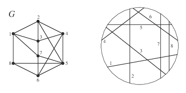
But still a few problems remain NP-complete in circle graphs, like -Colorability for [32], Hamiltonian Cycle [8], or Minimum Clique Cover [24]. In this article we study a variety of domination problems in circle graphs, from a parameterized complexity perspective. A dominating set in a graph is a subset such that every vertex in has at least one neighbor in . Some extra conditions can be imposed to a dominating set. For instance, if is a dominating set and is connected (resp. acyclic, an independent set, a graph without isolated vertices, a tree, a path), then is called a connected (resp. acyclic, independent, total, tree, path) dominating set. In the example of Fig. 1, vertices and (resp. , , and ) induce an independent (resp. connected) dominating set. The corresponding minimization problems are defined in the natural way. Given a set of graphs , the Minimum -Dominating Set problem consists in, given a graph , finding a dominating set of of minimum cardinality such that is isomorphic to some graph in . Throughout the article, we may omit the word “Minimum” when referring to a specific problem.
For an introduction to parameterized complexity theory, see for instance [10, 27, 15]. A decision problem with input size and parameter having an algorithm which solves it in time (for some computable function depending only on ) is called fixed-parameter tractable, or FPT for short. The parameterized problems which are -hard for some are not likely to be FPT [10, 27, 15]. A parameterized problem is in XP if it can be solved in time , for some (unrestricted) functions and . The parameterized versions of the above domination problems when parameterized by the cardinality of a solution are also defined naturally.
Previous work.
Dominating Set is one of the most prominent classical graph-theoretic NP-complete problems [17], and has been studied intensively in the literature. Keil [23] proved that Dominating Set, Connected Dominating Set, and Total Dominating Set are NP-complete when restricted to circle graphs, and Damian and Pemmaraju [9] proved that Independent Dominating Set is also NP-complete in circle graphs, answering an open question from Keil [23].
Hedetniemi, Hedetniemi, and Rall [21] introduced acyclic domination in graphs. In particular, they proved that Acyclic Dominating Set can be solved in polynomial time in interval graphs and proper circular-arc graphs. Xu, Kang, and Shan [34] proved that Acyclic Dominating Set is linear-time solvable in bipartite permutation graphs. The complexity status of Acyclic Dominating Set in circle graphs was unknown.
In the theory of parameterized complexity [15, 27, 10], Dominating Set also plays a fundamental role, being the paradigm of a -hard problem. For some graph classes, like planar graphs, Dominating Set remains NP-complete [17] but becomes FPT when parameterized by the size of the solution [2]. Other more recent examples can be found in -minor-free graphs [3] and claw-free graphs [7].
The parameterized complexity of domination problems has been also studied in geometric graphs, like -polygon graphs [11], multiple-interval graphs and their complements [13, 22], -gap interval graphs [16], or graphs defined by the intersection of unit squares, unit disks, or line segments [26]. But to the best of our knowledge, the parameterized complexity of the aforementioned domination problems in circle graphs was open.
Our contribution.
In this paper we prove the following results, which settle the parameterized complexity of a number of domination problems in circle graphs:
-
In Section 2, we prove that Dominating Set, Connected Dominating Set, Total Dominating Set, Independent Dominating Set, and Acyclic Dominating Set are -hard in circle graphs, parameterized by the size of the solution. Note that Acyclic Dominating Set was not even known to be NP-hard in circle graphs. The reductions are from -Colored Clique in general graphs.
-
Whereas both Connected Dominating Set and Acyclic Dominating Set are -hard in circle graphs, it turns out that Connected Acyclic Dominating Set is polynomial-time solvable in circle graphs. This is proved in Section 3.1.
-
Furthermore, if is a given tree, we prove that the problem of deciding whether a circle graph has a dominating set isomorphic to is NP-complete (Section 2.3) but FPT when parameterized by (Section 3.2). The NP-completeness reduction is from 3-Partition, and we prove that the running time of the FPT algorithm is subexponential. As a corollary of the algorithm presented in Section 3.2, we also deduce that, if has bounded degree, then deciding whether a circle graph has a dominating set isomorphic to can be solved in polynomial time.
Further research.
Some interesting questions remain open. We proved that several domination problems are -hard in circle graphs. Are they -complete, or may they also be -hard? On the other hand, we proved that finding a dominating set isomorphic to a tree can be done in polynomial time. It could be interesting to generalize this result to dominating sets isomorphic to a connected graph of fixed treewidth. Finally, even if Dominating Set parameterized by treewidth is FPT in general graphs due to Courcelle’s theorem [6], it is not plausible that it has a polynomial kernel in general graphs [5]. It may be the case that the problem admits a polynomial kernel parameterized by treewidth (or by vertex cover) when restricted to circle graphs.
2 Hardness results
In this section we prove hardness results for a number of domination problems in circle graphs. In order to prove the -hardness of the domination problems, we provide two families of reductions. Namely, in Section 2.1 we prove the hardness of Dominating Set, Connected Dominating Set, and Total Dominating Set, and in Section 2.2 we prove the hardness of Independent Dominating Set and Acyclic Dominating Set. Finally, we prove the NP-completeness for trees in Section 2.3.
For better visibility, some figures of this section have colors, but these colors are not indispensable for completely understanding the depicted constructions. Before stating the hardness results, we need to introduce the following parameterized problem, proved to be -hard in [13].
-Colored Clique Instance: A graph and a coloring of using colors. Parameter: . Question: Does there exist a clique of size in containing exactly one vertex from each color?
Note that in an instance of -Colored Clique, we can assume that there is no edge between any pair of vertices colored with the same color. Also, we can assume that for each , the number of vertices colored with color is the same. Indeed, given an instance , we can consider an equivalent instance obtained by putting together disjoint copies of , one for each permutation of the color classes.
In a representation of a circle graph, we will always consider the circle oriented anticlockwise. Given three points in the circle, by we mean that starting from and moving anticlockwise along the circle, comes before . In a circle representation, we say that two chords with endpoints and are parallel twins if , and there is no other endpoint of a chord between and , nor between and . Note that for any pair of parallel twins and , we can slide (resp. ) arbitrarily close to (resp. ) without modifying the circle representation.
2.1 Hardness of domination, and connected and total domination
We start with the main result of this section.
Theorem 2.1
Dominating Set is -hard in circle graphs, when parameterized by the size of the solution.
Proof
We shall reduce the -Colored Clique problem to the problem of finding a dominating set of size at most in circle graphs. Let be an integer and let be a -colored graph on vertices such that vertices are colored with color for all . For every , we denote by the vertices of color , with . Let us prove that has a -colored clique of size if and only if the following circle graph has a dominating set of size at most . We choose an arbitrary point of the circle as the origin. The circle graph is defined as follows:

-
We divide the circle into disjoint open intervals for , called sections. Each section is divided into disjoint intervals for , called clusters (see Fig. 2 for an illustration). Each cluster has particular points denoted by following the order of the circle. These intervals are constructed in such a way that the origin is not in a section.
-
Sections are numbered from to following the anticlockwise order from the origin. Similarly, the clusters inside each section are numbered from to .
-
For each , we add a chord with endpoints and , which we call the extremal chord of the -cluster of the -th section.
-
For each and , we add chords between the -th and the -th clusters of the -th section as follows. For each , we add two parallel twin chords, each having one endpoint in the interval of the -th cluster, and the other endpoint in the interval of the -th cluster. These chords are called inner chords (see Fig. 3 for an illustration). We note that the endpoints of the inner chords inside each interval can be chosen arbitrarily. The interval is the interval between and the point , and similarly is the interval between the point and .
-
We also add chords between the first and the last clusters of each section. For each and , we add a chord joining the point of the first cluster and the point of the last cluster of the -th section. For each , these chords are called the -th memory chords.
-
Extremal, inner, and memory chords will ensure some structure on the solution. On the other hand, the following chords will simulate the behavior of the original graph. In fact, the particular points in each cluster of the -th section will simulate the behavior of the vertices of color in . Let . The chords from the -th section to the -th section are between the -th cluster of the -th section and the -th cluster of the -th section. Between this pair of clusters, we add a chord joining the point (in the -th section) and the point (in the -th section) if and only if . We say that such a chord is called associated with an edge of the graph , and such chords are called outer chords. In other words, there is an outer chord in if the corresponding vertices are connected in .
Intuitively, the idea of the above construction is as follows. For each , among the clusters in the -th section, the first and the last one do not contain endpoints of outer chords, and are only used for technical reasons (as discussed below). The remaining clusters in the -th section capture the edges of between vertices of color and vertices of the remaining colors. Namely, for any two distinct colors and , there is a cluster in the -th section and a cluster in the -th section such that the outer chords between these two clusters correspond to the edges in between colors and . The rest of the proof is structured along a series of claims.
Claim 1
If there exists a -colored clique in , then there exists a dominating set of size in .
Proof
Assume that there is a -colored clique in and let us denote by the integer such that is the vertex of color in this clique. Let be the following set of chords. For each section , we add to the memory chord joining the points of the first and the last clusters. We also add in the outer chords associated with the edges of the -colored clique. The set contains chords: memory chords and outer chords. Let us prove that is a dominating set.
The extremal chords are dominated, since has exactly one endpoint in each cluster. Indeed, there is an endpoint in the first and the last cluster of section because of the memory chords of . There is an endpoint in the other clusters because of the outer chord associated with the edge of the -colored clique. The inner chords are also dominated. Indeed, for each section , the endpoint of the chord of is , for all clusters such that . Thus, for all , the inner chords between the intervals of the -th cluster and of the -th cluster are dominated by the chord of with endpoint in the -th section if , or by the chord of the -th section otherwise.
The outer chords are dominated by the memory chords of , since the outer chords have their endpoints in two different sections. Finally, the memory chords are also dominated by the outer chords of for the same reason.
In the following we will state some properties about the dominating sets in of size .
Claim 2
A dominating set in has size at least , and a dominating set of this size has exactly one endpoint in each cluster.
Proof
The interval of a chord linking and , with , is the interval . One can note that when chords have pairwise disjoint intervals, at least chords are necessary to dominate them.
The intervals of the extremal chords are disjoint by assumption. Since there are extremal chords, a dominating set has size at least . And if there is a dominating set of such size, it must have exactly one endpoint in each interval, i.e., one endpoint in each cluster.
Claim 3
A dominating set of size in contains no inner nor extremal chord.
Proof
Let be a dominating set in of size . It contains no extremal chords, since both endpoints of an extremal chord are in the same cluster, which is impossible by Claim 2. If contains an inner chord , the parallel twin of in is dominated by some other chord . But then intersect at most three clusters, which is again impossible by Claim 2.
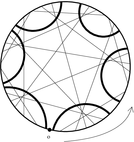
By Claim 3, a dominating set in of size contains only memory and outer chords. Thus, the unique (by Claim 2) endpoint of the dominating set in each cluster is one of the points , and we call it the value of a cluster. Fig. 4 illustrates the general form of a solution.
Claim 4
Assume that contains a dominating set of size . Then, in a given section, the value of a cluster does not increase between consecutive clusters.
Proof
Assume that in a given arbitrary section, the value of the -th cluster is . The inner chords between the interval of the -th cluster and the interval of the -th cluster have to be dominated. Since the value of the -th cluster is , they are not dominated in the -th cluster. Therefore, in order to ensure the domination of these chords, the value of the -th cluster is at most .
Claim 5
Assume that contains a dominating set of size . Then, for each , all the clusters of the -th section have the same value.
Proof
Let be such a dominating set. In a given section, the endpoints of in the first and the last clusters are endpoints of a memory chord, and for all , they link the point of the first cluster to the point of the last one. Thus, the first and the last clusters have the same value. Since by Claim 4 the value of a cluster decreases between consecutive clusters, the value of the clusters of the same section is necessarily constant.
The value of a section is the value of the clusters in this section (note that it is well-defined by Claim 5). The vertex associated with the -th section is the vertex if the value of the -th section is .
Claim 6
If there is a dominating set in of size , then for each pair with , the vertex associated with the -th section is adjacent in to the vertex associated with the -th section. Therefore, has a -colored clique.
Proof
Let and be two sections with , and let and be the vertices associated with these two sections, respectively. By Claim 5, the chord of the dominating set in the -th cluster of the -th section has a well-defined endpoint , and the chord of the dominating set in the -th cluster of the -th section has a well-defined endpoint . The vertex associated with the -th section is adjacent in to the vertex associated with the -th section. Indeed, the chords having endpoints in these clusters are exactly the chords between these two clusters, and there is a chord if and only if there is an edge between the corresponding vertices in .
Claims 1 and 6 together ensure that has a dominating set of size if and only if has a -colored clique. The reduction can be easily done in polynomial time, and the parameters of the problems are polynomially equivalent. Thus, Dominating Set in circle graphs is -hard. This completes the proof of Theorem 2.1.
From Theorem 2.1 we can easily deduce the -hardness of two other domination problems in circle graphs.
Corollary 1
Connected Dominating Set and Total Dominating Set are -hard in circle graphs, when parameterized by the size of the solution.
Proof
In the construction of Theorem 2.1, if there is a dominating set of size in , it is necessarily connected (see the form of the solution in Fig. 4). Indeed, the memory chords ensure the connectivity between all the chords with one endpoint in a section. Since there is a chord between each pair of sections, the dominating set is connected. Finally, note that a connected dominating set is also a total dominating set, as it contains no isolated vertices.
2.2 Hardness of independent and acyclic domination
We proceed to describe our second construction in order to prove parameterized reductions for domination problems in circle graphs.
Theorem 2.2
Independent Dominating Set is -hard in circle graphs.
Proof
We present a parameterized reduction from -Colored Clique in a general graph to the problem of finding an independent dominating set of size at most in a circle graph. Let be the input -colored graph with color classes . Let be the vertices belonging to the color class , in an arbitrary order. We proceed to build a circle graph by defining its circle representation. Let be a collection of disjoint intervals in the circle, which will we associated with the colors. For , we proceed to construct an induced subgraph of whose chords have all endpoints in the interval , which we visit from left to right. Throughout the construction, cf. Fig. 5 for an example with .

We start by adding two cliques on vertices and , with chords and , respectively, in the following way. The endpoints of and are placed in three disjoint subintervals of , such that the first subinterval contains, in this order, the left endpoints of . The second subinterval contains the right endpoints of and the left endpoints of , in the order . Finally, the third subinterval contains, in this order, the right endpoints of . The blue (resp. red) chords in Fig. 5 correspond to (resp. ).
For , we define the interval as the open interval between the right endpoint of and the left endpoint of ; cf. the thick intervals in Fig. 5. Such an interval will correspond to vertex of .
We also add two sets of parallel twin chords whose left endpoints are placed exactly before the left (resp. right) endpoint of (resp. ) and whose right endpoints are placed exactly after the left (resp. right) endpoint of (resp. ); cf. the green chords in Fig. 5. We call these chords parallel chords. This completes the construction of .
Finally, for each pair of vertices of such that and , we add to a chord between the interval in and the interval in ; cf. the dashed chords in Fig. 5. We call these chords outer chords. That is, the outer chords of correspond to non-edges of . This completes the construction of the circle graph .
We now claim that has a -colored clique if and only if has an independent dominating set of size at most .
Indeed, let first be a -colored clique in containing vertices , and let us obtain from an independent dominating set in . For , the set contains the two chords and from . Note that is indeed an independent set. For , since both and are cliques, all the chords in and are dominated by . Clearly, all parallel chords are also dominated by . The only outer chords with one endpoint in which are neither dominated by nor by are those with its endpoint in the interval . Let be such an outer chord, and suppose that the other endpoint of is in . As is a clique in , it follows that there is no outer chord in with one endpoint in and the other in , and therefore necessarily the chord is dominated either by or by .
Conversely, assume that has an independent dominating set with . Note that for , because of the two sets of parallel chords in , at least one of the chords in and at least one of the chords in must belong to , so . Therefore, it follows that and that contains in , for , a pair of non-crossing chords in and . Note that in each , the two chords belonging to must leave uncovered at least one of the intervals (corresponding to vertices) . Let and be two uncovered vertices in two distinct intervals and , respectively. By the construction of , it holds that the vertices and must be adjacent in , as otherwise the outer chord in between the intervals and would not be dominated by . Hence, a -colored clique in can be obtained by selecting in each any of the uncovered vertices.
The construction of Theorem 2.2 can be appropriately modified to deal with the case when the dominating set is required to induce an acyclic subgraph.
Theorem 2.3
Acyclic Dominating Set is -hard in circle graphs.
Proof
As in Theorem 2.2, the reduction is again from -Colored Clique. From a -colored , we build a circle graph that contains all the chords defined in the proof of Theorem 2.2, plus the following ones for each , (cf. Fig. 6 for an illustration): we add another set of parallel chords whose left (resp. right) endpoints are placed exactly before (resp. after) the right (resp. left) endpoint of (resp. ); cf. the middle green chords in Fig. 6. We call these three sets of chords parallel chords.

Furthermore, we add a clique with chords such that for the left (resp. right) endpoint of is placed exactly after the left (resp. right) endpoint of (resp. ). Finally, for each such a chord we add a parallel twin chord, denoted by . We call these chords distance chords, and their union is denoted by ; cf. the brown edges in Fig. 6. This completes the construction of . Note that a pair of chords and dominates all the distance chords in if and only if and do not cross, that is, if and only if .
We now claim that has a -colored clique if and only if has an acyclic dominating set of size at most .
Indeed, let first be a -colored clique in . An independent (hence, acyclic) dominating set in of size can be obtained from exactly as explained in the proof of Theorem 2.2. Note that in each , the distance chords in are indeed dominated by because the corresponding chords in and do not cross.
Conversely, assume that has an acyclic dominating set with . First assume that contains no outer chord. By the parallel chords in each (cf. the green chords in Fig. 6), it is easy to check that must contain at least two chords in each , and therefore we have that . We now distinguish several cases according to which two chords in a generic can belong to . Let . Because of the parallel chords, it is clear that only one , , or cannot contain both and . It is also clear that no parallel chord can be in . If and , let w.l.o.g. and . Since must dominate the twin chord , it follows by the construction of that , and therefore the chord is dominated neither by nor by (cf. Fig. 6), a contradiction. The case and is similar. Therefore, we may assume w.l.o.g. that and . Note that such a pair of chords and dominates all the distance chords in if and only if and do not cross. Hence, as in the proof of Theorem 2.2, for each , , the two chords belonging to leave at least one uncovered interval (corresponding to vertex ), and in order for all the outer chords in to be dominated, the union of the uncovered vertices must induce a -colored clique in . Therefore, if has an acyclic dominating set of size at most with no outer chord, then has a -colored clique. Note that in this case consists of an independent set.
Otherwise, the acyclic dominating set contains some outer chord. Assume w.l.o.g. that contains outer chords with at least one endpoint in each of (with , as each chord has two endpoints), and no outer chord with an endpoint in any of (only if ). By the arguments above, for it follows that contains exactly one chord in and exactly one chord in . For , in order for all the parallel chords in to be covered, must contain some chords in , , or . As by assumption , in at least one with , contains exactly one chord in , , or . By the construction of , this chord must necessarily be a distance chord, as otherwise some parallel chords in would not be dominated by (cf. Fig. 6). Assume w.l.o.g. that in only the distance chord and one outer chord outgoing from interval belong to . But then if (resp. ) the chord (resp. ) is not dominated by , a contradiction. We conclude that contains at least two outer chords in .
By a simple counting argument, as it follows that for , contains exactly one distance chord and two outer chords from each of (and, in particular, ). But then the subgraph of induced by the chords belonging to has minimum degree at least two, and therefore it contains a cycle, a contradiction to the assumption that is acyclic. Thus, cannot contain any outer chord, and the theorem follows.
2.3 NP-completeness for a given tree
The last result of this section is the NP-completeness when the dominating set is restricted to be isomorphic to a given tree.
Theorem 2.4
Let be a given tree. Then -Dominating Set is NP-complete in circle graphs when is part of the input.
Proof
We present a reduction from the 3-Partition problem, which consists in deciding whether a given multiset of integers can be partitioned into triples that all have the same sum . The 3-Partition problem is strongly NP-complete, and in addition, it remains NP-complete even when every integer in is strictly between and [17]. Let be an instance of 3-Partition, in which we can assume that the ’s are between and , and let be the desired sum. Note that we can also assume that is an integer, as otherwise is obviously a No-instance.
We proceed to define a tree and to build a circle graph that has a -dominating set if and only if is a Yes-instance of 3-Partition. Given , let be the rooted tree obtained from a root to which we attach a path with vertices, for ; see Fig 7(a) for an example with , , and . (In this figure, for simplicity not all the ’s are between and , but we assume that this fact is true in the proof.) Note that .
The circle graph is obtained as follows; see Fig 7(b) for the construction corresponding to the instance of Fig 7(a): We start with a chord that will correspond to the root of . Now we add parallel chords intersecting only with . These chords are called branch chords; cf. the green chords in Fig 7(b). We can assume that the endpoints of the branch chords are ordered clockwise in the circle. For , we add a chord incident only with . These chords are called pendant chords; cf. the blue chords in Fig 7(b), where for better visibility these chords have been depicted outside the circle. Finally, for , we add a chord whose first endpoint is exactly after the first endpoint of (in the anticlockwise order, starting from any of the endpoints of the root ), and whose second endpoint is exactly before the second endpoint of . These chords are called chain chords; cf. the red chords in Fig 7(b). Note that is adjacent to , and . This completes the construction of the circle graph . Each one of the connected components that remain in after the removal of and the parallel chords is called a block.

Let first be a Yes-instance of 3-Partition, and we proceed to define a -dominating set in . For , let be the -th triple of the 3-partition of ; in the instance of Fig 7(a), we have . We include the chord in , plus the following chords for each : For , we add to the branch chord plus, if , the chain chords for ; cf. the thick chords in Fig 7(c). It can be easily checked that is a -dominating set of .
Conversely, let be a -dominating set in , and note that we can assume that the root of has arbitrarily big degree. As the vertex of corresponding to the chord is the only vertex of of degree more than 6, necessarily belongs to , and corresponds to the root of .
We claim that contains no pendant chord. Indeed, by construction of , exactly of the branch chords are in , which dominate exactly pendant chords. As consists of disjoint paths, each attached to through a branch chord, the total number of chords in these paths which are not branch chords is . These pendant or chain chords must dominate the pendant chords that are not dominated by branch chords, which are also many. Assume that a pendant chord belongs to . Since is a tree, there must exist a path in between and one of the branch chords, say . Assume that contains chords, including but not . It is clear that is the only pendant chord contained in , as otherwise would have a cycle. Therefore, has chords and dominates exactly pendant chords that are not dominated by branch chords, which contradicts the fact that pendant or chain chords must dominate the pendant chords that are not dominated by branch chords. Hence, contains no pendant chord, so contains exactly chain chords.
Since is a tree, each path in made of consecutive chain chords intersects exactly one branch chord. As the ’s are strictly between and , each block has exactly 3 branch chords in . The fact that chain chords are missing between consecutive blocks assures the existence of a 3-partition of . More precisely, the restriction of to each block defines the integers belonging to each triple of the 3-partition of as follows. For a branch chord , let be the path in hanging from , which consists only of chain chords. Then, for each branch chord , the corresponding integer is defined by the number of vertices in plus one. By the above discussion, these triples define a 3-partition of . The theorem follows.
To conclude this section, it is worth noting here that -Dominating Set is -hard in general graphs. This can be proved by an easy reduction from Set Cover parameterized by the number of sets, which is -hard [28]. Indeed, let be a collection of subsets of a set , and the question is whether there exist at most subsets in whose union contains all elements of . We construct a graph as follows. First, we build a bipartite graph , where there is a vertex in (resp. ) for each subset in (resp. element in ), and there is an edge in between a vertex in and a vertex in if the corresponding subset contains the corresponding element. We add a new vertex , which we join to all the vertices in , and new vertices joined only to . It is then clear that has a dominating set isomorphic to a star with exactly leaves if and only if there is a collection of at most subsets in whose union contains all elements of .
3 Polynomial and FPT algorithms
In this section we provide polynomial and FPT algorithms for finding dominating sets in a circle graph which are isomorphic to trees. Namely, in Section 3.1 we give a polynomial-time algorithm to find a dominating set isomorphic to some tree. This algorithm contains the main ideas from which the other algorithms in this section are inspired. In Section 3.2 we modify the algorithm to find a dominating set isomorphic to a given tree in FPT time, the parameter being the size of . By carefully analyzing its running time, we prove that this FPT algorithm runs in subexponential time. It follows from this analysis that if the given tree has bounded degree (in particular, if it is a path), then the problem of find a dominating set isomorphic to can be solved in polynomial time.
3.1 Polynomial algorithm for trees
Note that, in contrast with Theorem 3.1 below, Theorem 2.3 in Section 2.2 states that, if is the set of all forests, then -Dominating Set is -hard in circle graphs. This is one of the interesting examples where the fact of imposing connectivity constraints in a given problem makes it computationally easier, while it is usually not the case (see for instance [4, 29]).
Theorem 3.1
Let be the set of all trees. Then -Dominating Set can be solved in polynomial time in circle graphs. In other words, Connected Acyclic Dominating Set can be solved in polynomial time in circle graphs.
Proof
Let be a circle graph on vertices and let be an arbitrary circle representation of . We denote by the set of intersections of the circle and the chords in this representation. The elements of are called points. Without loss of generality, we can assume that only one chord intersects a given point. Given two points , the interval is the interval from to in the anticlockwise order. Given four (non-necessarily distinct) points , with , by the region we mean the union of the two intervals and . Note that these two intervals can be obtained by “subtracting” the interval from the interval ; this is why we use the notation .
In the following, by size of a set of chords, we mean the number of chords in it, i.e., the number of vertices of in this set. We say that a forest of spans a region if each of , and is an endpoint of some chord in , and each endpoint of a chord of is either in or in . A forest is split by a region if for each connected component of there is exactly one chord with one endpoint in and one endpoint in . Given a region , a forest is -dominating if all the chords of with both endpoints either in the interval or in the interval are dominated by . A forest is valid for a region if it spans , is split by , and is -dominating.
Note that an -dominating forest with several connected components might not dominate some chord going from to . This is not the case if is connected, as stated in the following claim.
Claim 7
Let be a valid tree for a region . Then all the chords of with both endpoints in are dominated by .
Proof
All the chords with both endpoints either in or in are dominated by , since is -dominating. Hence we just have to prove that the chords with one endpoint in and one in are dominated by . Since spans , there are in a chord with endpoint and a chord with endpoint . Since is split by , there is a unique chord in with one endpoint in and one in . In , and are in the same connected component. Indeed, otherwise their connected components span two disjoint intervals of . But is the unique chord of with one endpoint in and one in , thus cannot connect these components. So, if is a tree, and are in the same connected component.
Thus for each point in , there is a chord of the connected component of and such that . Therefore, the chords with one endpoint in and one endpoint in are dominated.
We now state two properties that will be useful in the algorithm. Their correctness is proved below.
- T1
Let and be two valid forests for two regions and , respectively, such that . If there is no chord with both endpoints either in or in , then is valid for (see Fig. 8).
- T2
Let and be two valid forests for two regions and , respectively ( being possibly empty), and let be a chord such that , and such that there is no chord with both endpoints either in , or in , or in , or in . Then is a tree which is valid for . When is empty, we consider that correspond to the point . (see Fig. 8).
Roughly speaking, the intuitive idea behind this two properties is to reduce the length of the circle in which we still have to do some computation (that is, outside the valid regions), which will be helpful in the dynamic programming routine. Again, the proof is structured along a series of claims. Before verifying the correctness of Properties T1 and T2, let us first state a useful general fact.
Claim 8
Let be a region and let be a valid forest for . The chords with one endpoint in and one endpoint in are dominated by .
Proof
Let us now consider a chord with one endpoint in and one endpoint in . First assume that is in . Since is split by , there is a chord of with one endpoint in and one in , and such a chord dominates . Therefore, by symmetry, we can assume that is in . Since spans , there is a chord in with endpoint . Since is split by , there is a chord of , in the same connected component as the chord with endpoint , with one endpoint in and one endpoint in . If , then the chord is dominated by . Thus we can assume that . And note that by assumption, . But in , the chord with endpoint is connected to the chord , thus there is a chord of such that , and therefore the chord is dominated by , which achieves the proof of the claim.
Note that the proof of Claim 8 is symmetric, and then the same result is still true for the intervals and . Note also that the same result holds without the asumption that is -dominating.
Claim 9
Property T1 is correct.
Proof
Let us prove that is a forest and that it is valid for the region . For an illustration refer to Fig. 8. Since and span and respectively, all the endpoints of the chords of are in , and those of are in . Thus the order ensures that a chord of cannot cross of chord of . Therefore, is still a forest and the connected components of the union are precisely the connected components of and the connected components of .
Since spans , there is a chord of with endpoint and one chord with endpoint , and the same holds for and . Then spans the region .
Since is split by , there is exactly one chord per connected component between and , thus also between and . The same holds for . Thus each connected component of has exactly one chord with one endpoint in and the other one in . So is split by .
Let us now prove that is -dominating. Let us verify that all the chords in the interval are dominated by . By symmetry, the same will hold for the interval . All the chords with both endpoints in the interval are dominated by , and those with both endpoints in the interval are dominated by . By assumption, there is no chord in the interval . The chords with one endpoint in and one endpoint in are dominated by by Claim 8, and those with one endpoint in and one endpoint in are dominated by . Thus all the chords with both endpoints in are dominated by , which ensures that is -dominating.
Therefore, is valid for the region .
Claim 10
Property T2 is correct.
Proof
Let and be two valid forests for and for , respectively ( being possibly empty), and let be a chord with endpoints and , such that and such that there is no chord with both endpoints in either , or , or , or . For an illustration, refer also to Fig. 8.
First note that is a tree. Indeed, as in Claim 9, one can prove that is a forest with exactly one chord with one endpoint in and one endpoint in per connected component. Thus, the addition of ensures that is a tree.
Since and spans and respectively, spans . Indeed, there are chords intersecting and in , chords intersecting and in , and all the chords are strictly inside . Note that when the forest is empty, there is a chord intersecting , and thus the tree spans .
The tree spans , since there is exactly one chord with one endpoint in and one endpoint in , which is precisely the chord .
Let us prove that is -dominating. First note that the chords with one endpoint in and one endpoint in are dominated by . By symmetry, we just have to prove that the chords with both endpoints in are dominated by . By symmetry again, we just have to prove that the chords with both endpoints in are dominated. There is no chord with both endpoints in , the chords with both endpoints in are dominated by , since is -dominating. By Claim 8, the chords with one endpoint in and one endpoint in are dominated by , thus the chords with one endpoint in and one in are dominated.
Therefore, we conclude that is a valid tree for .
For a region , we denote by (resp. ) the least integer for which there is a valid forest (resp. tree) of size for . If there is no valid forest (resp. tree) for , we set (resp. ). Let us now describe our algorithm based on dynamic programming. With each region , we associate two integers and . Algorithm 1 below calculates these two values for each region. We next prove that and , and that Algorithm 1 computes the result in polynomial time.
Claim 11
For any region , (resp. ) if and only if (resp. ).
Proof
Let be a region such that . Therefore, there is a set of chords of size one which is valid for . Let be this chord. Since spans and , has endpoints . This implies that and , i.e., is precisely the chord . If , then , , and the chord exists, which corresponds exactly to the initialization of the algorithm. Conversely, it is clear that by definition the chord is valid for the region . Thus, if and only if . The same result holds for trees, since a forest of size one is a tree.
Claim 12
For any region , (resp. ).
Proof
The claim is true for the initialization, since if then . By induction it is still true for all integers , since Properties T1 and T2 are correct, and when a value is affected in the dynamic programming of Algorithm 1, one of the two properties is applied.
Claim 13
For any region , and .
Proof
Let us prove it by induction on . Claim 11 ensures that the result is true for . Assume that for all , if then and that if then .
Let us first prove that the induction step holds for trees. We now prove that if , then . Let be a valid tree of size for the region . Since spans , there is exactly one chord with one endpoint in and one endpoint in . Let be the restriction of to the chords with both endpoints in , and let be the restriction of to the chords with both endpoints in . Note that . Let (resp. ) be the points of the circle graph intersected by (resp. ) such that (resp. ), and (resp. ) are as near as possible from (resp. ) (see Fig. 9 for an example). Let us denote by (resp. ) the size of (resp. ). Note that .
Let us prove that is valid for , that is valid for , and that Property T2 can be applied to , , and the chord . By symmetry, we just have to prove that is valid. There are chords intersecting , by definition of , and chords intersecting since spans . The endpoints of the chords are in , since spans and are the nearest points from which are in . Thus spans .
If there is a connected component of with no chord from to , then cannot be a tree, since it would not be connected. If a connected component of has two chords from to , then has a cycle, which contradicts the fact that is a tree. Thus spans .
Let us prove that is -dominating. Indeed, if there is a chord with both endpoints in which is not dominated by , it cannot be dominated by and , since none of their endpoints is in this interval. Thus is not valid. Hence all the chords in the interval , and by symmetry also in the interval , are dominated by . Therefore is valid. By induction hypothesis, since the size of is at most , we have , and the same holds for .
Since is valid, one can note that there is no chord with both endpoint either in , or , or , or . Thus Property T2 can be safely applied and then , as we wanted to prove.
Let us now prove that the induction step also holds for forests. Let us now consider a forest for the region . If the forest has exactly one connected component, that is, if it is a tree, then the inequality holds by the first part of the induction.
Assume now that has at least two connected components. Let us now prove that if then . Let be a region with . This means that there exists a forest with one endpoint in , since spans . Since , has at least two connected components. Note that the case when is treated just above.
Since spans , all the endpoints of are in . Let be the connected component of the chord with endpoint . The point (resp. ) is the point of (resp. ) with an endpoint in , and such that there is no endpoint of after (resp. before ) in (resp. ). Let (resp. ) be the first endpoint of after in (resp. before in ).
Let us denote by the set (see Fig. 10 for an example). Let us prove that and are valid for and for , respectively. Since is -dominating, all the chords with both endpoints either in or in (resp. or ) are dominated by , thus by (resp. ). Therefore (resp. ) is -dominating (resp. -dominating). Thus, by induction hypothesis we have and . And since Property T1 can be applied for , by the safeness of Property T1, in Algorithm 1 we have .
Claims 12 and 13 together ensure that and that . Hence, by dynamic programming all the regions of a given size can be found in polynomial time. Let us now explain how we can verify if there is a dominating set isomorphic to some tree of a given size . This in particular will prove Theorem 3.1.
Claim 14
Let be a positive integer. There is a dominating tree of size at most in if and only if there is a region such that and such that there is no chord strictly contained in nor in .
Proof
Assume that there is a region with and no chord strictly contained in nor in . Then by Claim 8, all the chords with one endpoint in and one endpoint in are dominated, and the same holds for the couple . All the chords with both endpoints in are dominated by Claim 7, as is valid for . Since by assumption there is no chord strictly contained in and in , all the chords of the circle graph are dominated, as by assumption there is no chord in the other intervals. Thus, is a dominating set.
Conversely, let be a dominating tree of size . Let be a chord of which disconnects . Thus has at least two connected components and . Let be the two extremities of the first one, and let be the extremities of the other ones (see Fig. 9 for an illustration). Let us prove that . Indeed, is a tree by assumption, by definition it spans , it spans since the chord is the unique chord from to , and it is -dominating since is a dominating tree. In addition, since is a dominating tree, there is no chord with both endpoints either in the interval or in , as otherwise such a chord would not be dominated by .
By dynamic programming, Algorithm 1 computes in polynomial time the regions for which there is a valid tree of any size from to . Given a region with , we just have to verify that there are no chords in the intervals and , which can clearly be done in polynomial time. One can easily check that Algorithm 1 runs in time , but we did not make any attempt to improve its time complexity. This completes the proof of Theorem 3.1.
As Algorithm 1 computes the regions for which there is a valid tree of any size from to , it can be slightly modified to obtain the following corollary.
Corollary 2
Let be the set of all trees of size exactly . Then -Dominating Set can be solved in polynomial time in circle graphs.
3.2 FPT algorithm for a given tree
It turns out that when we seek a dominating set isomorphic to a given fixed tree , the problem is FPT parameterized by . In order to express the running time of our algorithm, and to prove that it is subexponential in , we need some definitions. Let be a tree, and let us root at an arbitrary vertex . Let be a vertex of . We denote by the subtree of induced by and the descendants of in the rooted tree. Let be the children of in the tree rooted at . We define as the forest , which we consider as a multiset with elements , where we consider two isomorphic trees and as the same element. Suppose that contains exactly non-isomorphic trees , and that for , there are exactly trees in which are isomorphic to (note that ). We define the following parameter, which corresponds to the number of non-isomorphic sub(multi)sets of the multiset :
Finally, we also define the following three parameters:
Let . Note that for any tree , we easily have that , and that if has maximum degree at most , then it holds that (by choosing to be a leaf of ). In particular, if is a path on vertices, is holds that . In the following proposition we upper-bound the parameter , seen as a function of , which will allow us to prove that the running time of the algorithm in Theorem 3.2 is subexponential.
Proposition 1
.
Proof
Let be an integer and let be a tree which maximizes , i.e., a tree for which . Let be a root of maximizing , and let be a vertex of such that maximizes . We claim that we can assume that . Note that if , then it holds that , as on the left-hand side we have one more child of that contributes to . Assume for contradiction that . Then, by the previous inequality it holds that , contradicting the choice of . Therefore, we assume henceforth that .
Let be all the non-isomorphic rooted trees of sorted by increasing size (where size means number of vertices). As defined before, we denote by the number of occurrences of in . By simplicity in the sequel, let us denote by the size of . We first want to find an upper bound on .
We will need the fact that the number of unlabeled rooted trees of size is asymptotically equal to , where and (see for instance [14, Chapter VII.5]). It follows that there exist two constants and a constant such that for all , the number of unlabeled rooted trees of size satisfies
| (1) |
Claim 15
There exists a constant such that .
Proof
Let us first prove by contradiction that all the trees of size at most appear in . Assume that there is a tree of size at most which is not in . Let be the same tree as , rooted at , except that we replace all the occurrences of in by occurrences of . Since the size of is at most , contains strictly less vertices, say , than . Thus in order to have vertices, we attach to the root of new trees isomorphic to the singleton-tree. Note that has also size . Let us calculate the difference between and . Note that by maximality of , we have . For all such that is not the singleton-tree, by construction the number of trees isomorphic to in in is equal to the number of occurrences of in in . Thus for all when is not the singleton-tree. Since, by construction, there are the same number of occurrences of in and of in , we have . Thus the only difference between and is the term corresponding to the singleton-tree. If the number of occurrences of the singleton-tree in is , then the number of occurrences of the singleton-tree in is . Thus , which contradicts the maximality of .
Thus, we can assume that all the non-isomorphic rooted trees of size at most appear in . By Equation (1), there are at least non-isomorphic rooted trees of size . Therefore, if there is a tree of size in , then necessarily
Note that, in particular, we have that for large enough. Indeed, when we replace by , the inequality is satisfied. In the following, when we write we mean .
Since one can easily check that the number of rooted trees of size at most is less that the number of rooted trees of size exactly , and since has size , by the previous inequalities we have
where the last inequality is a consequence of the fact that . Thus, there exists a constant, called again for simplicity, such that , as we wanted to prove.
We now state a useful claim.
Claim 16
Let be some real variables and let be the polynomial such that . Under the constraint , the polynomial is maximized when for all .
Proof
Assume for contradiction that this is not the case. Then by symmetry we can assume that . Thus there exists another value, say , such that . Let . To compare the two values of the polynomial, we just have to compare the product . One can easily verify that , contradicting the fact that the polynomial was maximized.
Claim 16 ensures that is maximized when all the ’s are equal. Since contains vertices and since each tree contains at least one vertex, it holds that . Thus the function is maximized when we have for all , i.e.,
Claim 17
Let be a large enough integer. The real function is increasing in the interval .
Proof
The derivative of the function is the following
Note that the first term is always a positive function. We also have . Thus we have when is large enough, since .
We are now ready to state Theorem 3.2, which should be compared to Theorem 2.4 in Section 2.3. We use Proposition 1 to conclude that the running time is subexponential.
Theorem 3.2
Let be a given tree. There exists an FPT algorithm to solve -Dominating Set in a circle graph on vertices, when parameterized by , running in time . In particular, if has bounded degree, -Dominating Set can be solved in polynomial time in circle graphs.
Proof
The idea of the proof is basically the same as in the proof of Theorem 3.1. The main difference is that in the proof of Theorem 3.1, when Properties T1 or T2 are satisfied, we can directly apply them and still obtain a forest or a tree. In the current proof, when we make the union of two forests, we have to make sure that the union of the two forests is still a subforest of , and that we can correctly complete it to obtain the desired tree . For obtaining that, we will apply the two properties stated below, whenever it is possible to create forests which are induced by the children of the same vertex of . Let us first give some intuition on the algorithm.
In the following we consider the tree rooted at an arbitrary vertex . Let be some vertices of which are children of the same vertex . The subforest of induced by , denoted by , is the forest .
Roughly speaking, the idea of the algorithm is to exhaustively seek, for each region and any possible subforest of for every vertex in , a valid forest for isomorphic to , and then try to grow it until hopefully obtaining the target tree . Note that if a vertex of has children, there are a priori possible subsets of children of , which define possible types of subforests in . But the key point is that if some of the trees in are isomorphic, some of the choices of subsets of subforests will give rise to the same tree. In order to avoid this redundancy, for each vertex of , we partition the trees in into isomorphism classes, and then the choices within each isomorphism class reduce to choosing the multiplicity of this tree, which corresponds to the parameter (as we may not choose any copy of it) defined before the statement of Proposition 1. Note that carrying out this partition into isomorphism classes can be done in polynomial time (in ) for each vertex of , using the fact that one can test whether two rooted trees and with vertices are isomorphic in time [1].
Therefore, if we proceed in this way, the number of such subforests for each vertex is at most . As we repeat this procedure for every node of , the cost of this routine per vertex is at most . And as we chose the root arbitrarily, it follows that the function can be upper-bounded by , which in turn can be upper-bounded by , which is a subexponential function by Proposition 1. We would like to note that this step is the unique non-polynomial part of the algorithm.
Let us now explain more precisely the outline of the algorithm. An induced subtree of the input circle graph is valid for a region and a tree , if it is valid for , and if, in addition, there is an isomorphism between and for which the unique chord between and corresponds to . A forest is valid for a region and , if it is valid for , and if there is an isomorphism between and for which the unique chord between and of each connected component corresponds to vertex . Let us now state the two properties that correspond to Properties T1 and T2 of Theorem 3.1.
- F1
Let and be two valid forests for and , and for and , respectively. Assume in addition that . Assume also that, for all , , the vertices and are pairwise distinct and are children of the same vertex of . If there is no chord with both endpoints either in or in , then is valid for and .
- F2
Let and be two valid forests for and , and for and , respectively ( being possibly empty), and let be a chord of the input graph . Assume that and that there is no chord with both endpoints either in , or in , or in , or in . Assume also that there exists a vertex of with exactly children Then is a tree which is valid for and . When is empty, we consider that correspond to the point .
In the proof of Theorem 3.1, we have seen that the validity of the corresponding regions is satisfied. Thus, we just have to verify that the tree or the forest which is created is isomorphic to the target tree , and that the chords with one endpoint in each side are children of the same vertex. The union of the two isomorphisms, and the fact that the chords with one endpoint in both sides are the children of , ensures that both properties are true. Indeed, for example for Property F2, since the chords with one endpoint in each interval are exactly the children of , it holds that the chord corresponding to the vertex intersects exactly its children.
For each region and each tree , we define a boolean variable , which is set to ‘true’ if and only if there is a valid tree for and . For each region and each forest , we define a boolean variable which is set to true if and only if there is a valid forest for and . (For the sake of simplicity, we distinguish between trees and forests, but we would like to stress that it is not strictly necessary for the algorithm.)
By a dynamic programming similar to Algorithm 1 in Theorem 3.1, we can compute all the regions and all vertices of for which (and the same for forests). If there is a region for which , and such that there is no chord with both endpoints either in or in , then the tree dominates all the chords in the input circle graph . Indeed, the safeness of Properties F1 and F2 ensures that there is a valid tree isomorphic to for the region . And Claim 14 in the proof of Theorem 3.1 ensures that this tree is indeed a dominating tree.
Note that, indeed, the unique non-polynomial step of the algorithm consists in generating the collection of non-isomorphic subforests, which are at most many. Thus, the dynamic programming algorithm runs in time . Again, we did not make any effort to optimize the degree of the polynomial in the running time.
Acknowledgment. We would like to thank Sylvain Guillemot for stimulating discussions that motivated some of the research carried out in this paper.
References
- [1] A. V. Aho, J. E. Hopcroft, and J. D. Ullman. The Design and Analysis of Computer Algorithms. Addison-Wesley, 1974.
- [2] J. Alber, H. L. Bodlaender, H. Fernau, T. Kloks, and R. Niedermeier. Fixed Parameter Algorithms for Dominated Set and Related Problems on Planar Graphs. Algorithmica, 33(4):461–493, 2002.
- [3] N. Alon and S. Gutner. Kernels for the Dominating Set Problem on Graphs with an Excluded Minor. Electronic Colloquium on Computational Complexity (ECCC), 15(066), 2008.
- [4] O. Amini, D. Peleg, S. Pérennes, I. Sau, and S. Saurabh. Degree-Constrained Subgraph Problems: Hardness and Approximation. In Proc. of the 6th Workshop on Approximation and On-line Algorithms (ALGO/WAOA), volume 5426 of LNCS, pages 29–42, 2008.
- [5] H. L. Bodlaender, R. G. Downey, M. R. Fellows, and D. Hermelin. On problems without polynomial kernels. Journal of Computer and System Sciences, 75(8):423–434, 2009.
- [6] B. Courcelle. The monadic second-order logic of graphs: definable sets of finite graphs. In In Proc. of the 14th International Workshop on Graph-theoretic Concepts in Computer Science (WG), number 344 in LNCS, pages 30–53, 1988.
- [7] M. Cygan, G. Philip, M. Pilipczuk, M. Pilipczuk, and J. O. Wojtaszczyk. Dominating set is fixed parameter tractable in claw-free graphs. Theoretical Computer Science, 412(50):6982–7000, 2011.
- [8] P. Damaschke. The Hamiltonian Circuit Problem for Circle Graphs is NP-Complete. Information Processing Letters, 32(1):1–2, 1989.
- [9] M. Damian-Iordache and S. V. Pemmaraju. Hardness of approximating independent domination in circle graphs. In 10th International Symposium on Algorithms and Computation (ISAAC), volume 1741 of LNCS, pages 56–69, 1999.
- [10] R. G. Downey and M. R. Fellows. Parameterized Complexity. Springer-Verlag, New York, 1999.
- [11] E. S. Elmallah and L. K. Stewart. Independence and domination in polygon graphs. Discrete Applied Mathematics, 44(1-3):65–77, 1993.
- [12] S. Even and A. Itai. Queues, stacks and graphs. In A. Press, editor, Theory of Machines and Computations, pages 71–86, 1971.
- [13] M. R. Fellows, D. Hermelin, F. A. Rosamond, and S. Vialette. On the parameterized complexity of multiple-interval graph problems. Theoretical Computer Science, 410(1):53–61, 2009.
- [14] P. Flajolet and R. Sedgewick. Analytic Combinatorics. Cambridge University Press, 2009.
- [15] J. Flum and M. Grohe. Parameterized Complexity Theory. Springer Verlag, 2006.
- [16] F. Fomin, S. Gaspers, P. Golovach, K. Suchan, S. Szeider, E. Jan Van Leeuwen, M. Vatshelle, and Y. Villanger. -Gap interval Graphs. To appear in the Proc. of the 10th Latin American Theoretical INformatics Symposium (LATIN), available at http://arxiv.org/abs/1112.3244, 2012.
- [17] M. Garey and D. Johnson. Computers and Intractability. W.H. Freeman, San Francisco, 1979.
- [18] F. Gavril. Algorithms for a maximum clique and a maximum independent set of a circle graph. Networks, 3:261–273, 1973.
- [19] F. Gavril. Minimum weight feedback vertex sets in circle graphs. Information Processing Letters, 107(1):1–6, 2008.
- [20] E. Gioan, C. Paul, M. Tedder, and D. Corneil. Circle Graph Recognition in Time . Manuscript available at http://arxiv.org/abs/1104.3284, 2011.
- [21] S. M. Hedetniemi, S. T. Hedetniemi, and D. F. Rall. Acyclic domination. Discrete Mathematics, 222(1-3):151–165, 2000.
- [22] M. Jiang and Y. Zhang. Parameterized Complexity in Multiple-Interval Graphs: Domination. In Proc. of the 6th International Symposium on Parameterized and Exact Computation (IPEC), volume 7112 of LNCS, pages 27–40, 2011.
- [23] J. M. Keil. The complexity of domination problems in circle graphs. Discrete Applied Mathematics, 42(1):51–63, 1993.
- [24] J. M. Keil and L. Stewart. Approximating the minimum clique cover and other hard problems in subtree filament graphs. Discrete Applied Mathematics, 154(14):1983–1995, 2006.
- [25] T. Kloks. Treewidth of circle graphs. International Journal of Foundations of Computer Science, 7(2):111–120, 1996.
- [26] D. Marx. Parameterized complexity of independence and domination on geometric graphs. In Proc. of the 2nd International Workshop on Parameterized and Exact Computation (IWPEC), volume 4169 of LNCS, pages 154–165, 2006.
- [27] R. Niedermeier. Invitation to Fixed-Parameter Algorithms. Oxford University Press, 2006.
- [28] A. Paz and S. Moran. Nondeterministic polynomial optimization problems and their approximations. Theoretical Computer Science, 15:251–277, 1981.
- [29] J. Rué, I. Sau, and D. M. Thilikos. Dynamic Programming for Graphs on Surfaces. In Proc. of the 37th International Colloquium on Automata, Languages and Programming (ICALP), volume 6198 of LNCS, pages 372–383, 2010.
- [30] N. A. Sherwani. Algorithms for VLSI Physical Design Automation. Kluwer Academic Press, 1992.
- [31] J. Spinrad. Recognition of circle graphs. Journal of Algorithms, 16(2):264–282, 1994.
- [32] W. Unger. On the -Colouring of Circle-Graphs. In Proc. of the 5th Annual Symposium on Theoretical Aspects of Computer Science (STACS), volume 294 of LNCS, pages 61–72, 1988.
- [33] W. Unger. The Complexity of Colouring Circle Graphs (Extended Abstract). In Proc. of the 9th Annual Symposium on Theoretical Aspects of Computer Science (STACS), volume 577 of LNCS, pages 389–400, 1992.
- [34] G. Xu, L. Kang, and E. Shan. Acyclic domination on bipartite permutation graphs. Information Processing Letters, 99(4):139–144, 2006.