Mathematical diffraction of aperiodic structures†
Michael Baakea and Uwe Grimmb
Kinematic diffraction is well suited for a mathematical approach via measures, which has substantially been developed since the discovery of quasicrystals. The need for further insight emerged from the question of which distributions of matter, beyond perfect crystals, lead to pure point diffraction, hence to sharp Bragg peaks only. More recently, it has become apparent that one also has to study continuous diffraction in more detail, with a careful analysis of the different types of diffuse scattering involved. In this review, we summarise some key results, with particular emphasis on non-periodic structures. We choose an exposition on the basis of characteristic examples, while we refer to the existing literature for proofs and further details.
1 Introduction
Diffraction techniques have dominated the structure analysis of solids for the last century, ever since von Laue and Bragg employed X-ray diffraction to determine the atomic structure of crystalline materials. Despite the availability of direct imaging techniques such as electron and atomic force microscopy, diffraction by X-rays, electrons and neutrons continues to be the method of choice to detect order in the atomic arrangements of a substance; see Cowley’s book35 and references therein for background.
In its full generality, the diffraction of a beam of X-rays, electrons or neutrons from a macroscopic piece of solid is a complicated physical process. It is the presence of inelastic and multiple scattering, prevalent particularly in electron diffraction, which makes it essentially impossible to arrive at a complete mathematical description of the process. Here, we restrict to kinematic diffraction in the far-field or Fraunhofer limit. In this case, powerful tools of harmonic analysis are available to attack the direct problem of calculating the (kinematic) diffraction pattern of a given structure.
In contrast, the inverse problem of determining a structure from its diffraction intensities is extremely involved. A diffraction pattern rarely determines a structure uniquely, as there can be homometric structures sharing the same autocorrelation (and hence the same diffraction).103, 57, 9, 54 We are far away from a complete understanding of the homometry classes of structures, in particular if the diffraction spectrum contains continuous components. At present, a picture is emerging, based on the analysis of explicit examples, which highlight how large the homometry classes may be.

Originally, much of the effort concentrated on the pure point part of diffraction, also called the Bragg diffraction, for the case of ordinary (periodic) crystals, and later also for incommensurate phases. Following the discovery of quasicrystals118, 70, 79, 92 with their beautiful diffraction patterns, such as the one shown in Figure 1, a new mathematical approach was required. The associated paradigm shift also re-opened the discussion of what possible manifestations of order and disorder in solids there are, and how these can be detected and quantified. While diffraction is one measure of order, the existence of homometric structures of varying entropy11, 14 shows its limitations, as there are completely deterministic systems which cannot be distinguished from a randomly disordered system on the basis of pair correlations alone. Increasingly, the continuous or diffuse part of the diffraction is attracting attention,133, 135, 40 not the least because improved experimental techniques make the diffuse part accessible. Improving our understanding of diffuse diffraction is desirable, in particular in view of the implications on disorder.

The most successful approach to describe the structure of incommensurate crystals and quasicrystals employs additional dimensions. By embedding the ideal structure into a higher-dimensional ‘superspace’, it is possible to recover periodicity in the higher-dimensional space, and this picture can be extended to cover certain aspects of random tilings as well. The standard tilings used to model the structure of quasicrystals are obtained in this way; for instance, the Penrose tiling104 shown in Figure 2 can be described as a projection19 of a slice through the four-dimensional root lattice . Such structures, or their equivalent point sets, are called cut and project sets or model sets, and we shall discuss further examples below. Note that the Penrose tiling also possesses aperiodic, perfect local rules (or matching rules75, 121, 52), as well as an inflation symmetry. The local rules can be implemented as arrow decorations on the edges of the two rhombic prototiles, which, within any admissible patch, have to agree on all edges. These local rules are aperiodic in the sense that they are incompatible with any periodic tiling. They are perfect because they specify precisely the class of the rhombic Penrose tilings, in the sense that all space-filling tilings obeying these rules are locally indistinguishable (LI) from the rhombic Penrose tiling, the latter defined as a fixed point tiling of an inflation rule.
It is worth noting that, while the lattice of periods of a periodic crystal is unique (though the choice of unit cell is not), there is considerable freedom in the choice of the building blocks of aperiodic tilings. In the case of the Penrose tiling, there exist a number of equivalent versions (in the sense25, 4, 16 of mutual local derivability), such as the Penrose pentagon tiling or the kite and dart tiling. One can even go beyond tilings and consider coverings of space.80 In the case of the Penrose tiling, Gummelt’s decagon covering58 with a single cluster (and overlap rules encoded by the shading) has proved very popular, because it allows the description of a quasicrystal structure in terms of a single fundamental building block. The three allowed (pairwise) overlaps of the marked decagons, shown in Figure 3, are characterised by matching decorations. Figure 4 shows a patch of a corresponding covering, which is mutually locally derivable (MLD) with the Penrose tiling of Figure 2.58, 59 This covering also has an interpretation in terms of ‘maxing rules’,72, 61, 49 where maximisation of one type of specified cluster leads to the Penrose rhombus tiling (up to zero density deviations).72 Covering rules of either type have become quite fashionable in materials science.109, 124 For more examples on tilings, in particular on substitution tilings, we refer to the online Tilings Encyclopedia.60 For the early development of the field, the reprint volume by Steinhardt and Ostlund123 is still a valuable source.


This review attempts to present an overview of the development of mathematical diffraction theory in the 30 years since the discovery of quasicrystals by Shechtman et al.118 While we aim to provide the reader with a flavour of the mathematical methods and assumptions, we will not dive deeply into the technical details. In particular, we will not present any formal proofs, though we do state several non-trivial results explicitly. We refer to our recent review13 and our forthcoming book,16 and the references contained therein, for more details on the rigorous mathematical treatment. Three complementary review volumes97, 22, 3 with mathematical articles are also highly recommended. Here, we select examples that are both characteristic and somewhat supplementary to previous presentations.
In Section 2, we start with a concise summary of the systematic approach using measures (in the mathematical sense, such as Lebesgue measure , which is used to measure volume in Euclidean space), which was pioneered in this context by Hof.67, 68, 69 We first apply this approach to the diffraction of perfect crystals in Section 3, and then discuss the case of mathematical quasicrystals based on a cut and project scheme in Section 4. Like perfect (or idealised) crystals, these systems are pure point diffractive, which means that the diffraction pattern consists of sharp (Bragg) peaks only. Afterwards, in Section 5, we proceed to systems with continuous diffraction, covering both the case of singular continuous and absolutely continuous diffraction by means of representative examples, including a probabilistic model for thermal fluctuations. In particular, we consider random tilings, which are relevant because most quasicrystalline materials show entropic stabilisation and therefore are expected to include configurational disorder.
2 Methods and general results
For a satisfying mathematical approach, we should exclude any boundary effects, and hence consider infinite systems that represent the scattering medium. Traditionally, there are two seemingly contradictory ways to describe a system, either in terms of functions which represent the density of the scattering medium, or by lattices or, more generally, tilings of space, whose decorations mimic the atomic positions. This dichotomy has sparked some rather fierce disputes between the tiling school and the density function school, in particular in the years following the discovery of quasicrystals. However, the two viewpoints can be reconciled by embedding them into a more general frame. One way of doing that is to introduce measures, which comprise (almost) periodic functions and tilings as special cases. As measures quantify distributions in spaces, this approach is in fact very natural, and well suited to describe both the distribution of matter in the scattering medium and the distribution of (scattered) intensity in space. We therefore start by briefly introducing the concepts and main properties that will be needed in our context.
2.1 Measures, convolutions and Fourier transforms
Due to the Riesz-Markov representation theorem,108 it is possible to think of a measure as a linear functional, i.e., as a linear map that associates a number to each function from an appropriate space. A (complex) measure on is then a linear functional (with values in the complex numbers ) on the space of complex-valued, continuous (test) functions of compact support, subject to the condition that, for every compact set , there is a constant such that
for all test functions with support in . Here, is the supremum norm of .
We write or for the measure of a function , and for the measure of a set , where
denotes the characteristic function of the set .
If is a complex measure, the conjugate of is the measure which is defined by . A measure is called real (or signed), when , and it is called positive when for all . For every measure , there is a smallest positive measure, denoted by , such that for all non-negative . This is called the total variation (or absolute value) of . A measure is called finite or bounded, if is finite, otherwise it is called unbounded. As we want to describe infinite point sets in space, we usually deal with the latter case, but we will assume that measures are translation bounded. This means that, for any compact set , the total variation satisfies
so wherever you move your compact set , its total variation measure is always finite.
2.2 Autocorrelation and diffraction measures
If is a point set that is a Delone set (a set where points neither get arbitrarily close nor so sparse that it accommodates arbitrarily large empty balls), the corresponding Dirac comb34
is a translation bounded measure, where is the normalised (Dirac) point measure at (so , or, in the formal notation used in physics, ). In what follows, we use such Dirac combs to represent the scattering medium, possibly with (in general complex) scattering weights at position . The corresponding weighted Dirac comb is denoted as
If is a translation bounded measure, the corresponding diffraction measure is the Fourier transform of the autocorrelation measure, where we shall assume that the latter exists. In any given example, this has to be verified, of course. The autocorrelation measure of is defined as the limit
| (1) |
where denotes the open ball of radius around . By we denote the restriction of to the ball . For a measure , its ‘flipped-over’ version is defined via , where . The operation is the ordinary convolution of measures, which is a generalisation of the standard convolution of integrable functions,
For finite measures and on , it is defined by
for any function , which is then again a finite measure. The volume-averaged convolution (also called the Eberlein convolution, in analogy to a similar approach51 in the theory of almost periodic measures) is needed in Eq. (1), because itself is generally an unbounded measure and the direct convolution is not defined. For example, if denotes the standard Lebesgue measure (for volume), is not defined, while .
If the autocorrelation measure of exists, its Fourier transform does as well, and is a translation bounded, positive measure, called the diffraction measure of . It corresponds to the kinematic scattering intensity observed in an experiment in the sense that it quantifies how much scattering intensity reaches a given volume in -space. Relative to Lebesgue measure , the diffraction measure has a unique decomposition108
into its pure point part (the Bragg peaks, of which there are at most countably many), its absolutely continuous part (the diffuse background scattering, which has a locally integrable density relative to ) and its singular continuous part (which simply means anything that remains, which is nothing in many standard cases considered in crystallography). Each of the three terms is again a positive measure. Singular continuous measures are weird objects: they give no weight to single points, but are still concentrated to an (uncountable!) set of zero Lebesgue measure. A well-known example is the probability measure for the classic middle-thirds Cantor set,108 with the ’Devil’s stair case’ as its distribution function, which is constant almost everywhere; see Figure 5. Singular continuous diffraction does occur in realistic models though,65 and should not be disregarded.

3 Diffraction of perfect crystals
In our setting, a perfect (infinite) crystal in -space is a lattice-periodic (discrete) structure. It is defined by its lattice of periods and the decoration of a fundamental domain of , which together completely specify the distribution of scatterers in space. It is therefore described by a crystallographic measure
| (2) |
where is a finite measure. The latter can be chosen as the restriction of to a fundamental domain of . Depending on the nature of , the resulting measure can be pure point or continuous (for instance, if is the constant measure on the fundamental domain, would be proportional to Lebesgue measure), or a mixture of both types. One can think of the Dirac comb as implementing the lattice periodicity, while describes the distribution of scatterers in a fundamental domain of .
The autocorrelation of the crystallographic measure of Eq. (2) is given by
| (3) |
which follows by using the relation together with . Here, denotes the density (per unit volume) of the lattice , which is the reciprocal of the volume of its fundamental domain. Consequently, is also a -periodic measure. In order to obtain the corresponding diffraction measure, we need to know how to calculate the Fourier transform of lattice-periodic measures.
3.1 Poisson’s summation formula
A powerful tool for the Fourier analysis of lattice-periodic measures is the Poisson summation formula (PSF). For a lattice (which means that is a discrete subgroup of such that the factor group is compact), the Fourier transform of the corresponding Dirac comb is
| (4) |
where denotes the dual or reciprocal lattice of . The latter is defined by
Here and below, denotes the scalar product of . Note that sometimes a factor is included in the definition of the reciprocal lattice, which we prefer to incorporate in our definition of the Fourier transform. For a suitable function , our convention for Fourier transform is
where and again denotes their scalar product. The Fourier transform of a positive definite measure (which means that holds for all ) is defined as the unique extension108, 29 of the Fourier transform of functions. It is conveniently defined in the setting of tempered distributions,108 which provide concrete means to calculate the transforms.
By the Bochner-Schwartz theorem,108 the diffraction measure is then a translation bounded positive measure. In addition, we will make use of the convolution theorem for measures. This states that if is a finite measure and a translation bounded measure on , the convolution exists and is a translation bounded measure.29 If is not only a tempered distribution, but itself also a measure, one has the convolution identity . The latter is then again a measure, which is absolutely continuous relative to , because is a bounded, uniformly continuous function on in this case.
3.2 Diffraction of crystallographic structures
Using the PSF together with the convolution theorem, the Fourier transform of the crystallographic autocorrelation measure of Eq. (3) can be calculated as
| (5) |
Clearly, this is a pure point measure, concentrated on the dual lattice . Note that is a uniformly continuous and bounded function that is evaluated only at points of the dual lattice . While different admissible choices for the measure (describing the same system) lead to different such functions, they agree on all points of , so that the result does not depend on this choice. If for some , one calls this an extinction. Extinctions are characteristic features of further symmetries, also of generalised type.
3.3 Planar -phases
Let us consider an interesting example in some detail. Starting from a checker board, viewed as a decoration of the square lattice, we assume that the grey squares are stiff (or solid), while the white squares are empty. One can now twist the structure by rotating the grey squares alternately in opposite directions by an angle ,
![[Uncaptioned image]](1205.3633v1/sigmadef.png) |
This way, a new periodic structure emerges where the white squares are deformed into congruent rhombuses. This structure is the lattice-periodic repetition of the motif above, and resembles a planar -phase and related quasicrystal approximants.70 A couple of examples are shown in Figure 6. The second is related to structures found in -fold symmetric quasicrystals.70

We consider the associated Dirac comb
obtained by placing a normalised point (or Dirac) measure at each vertex point. Here, we have and , while denotes the vertex set of the unit square . The corresponding diffraction measure is obtained via Eq. (5) as
with denoting the scalar product in .

When (which means we are back to the square lattice), this expression reduces to , as it must, while inserting leads to , which reflects the double weight of the point measures at each vertex in this limit. For angles with irrational, one has extinctions precisely for all wave vectors with and . When is rational, there are further extinctions, which can be calculated from the explicit formula for the diffraction measure .
The diffraction patterns for the two examples ( and ) from Figure 6 are illustrated in Figure 7. A Bragg peak is represented by a dot that is centred at the peak position and that has an area proportional to the intensity. This choice resembles the experimental situation in a reasonable way. Both patterns are non-periodic, due to the incommensurate positions of the points in the fundamental cell. While all Bragg peaks are located at positions of the corresponding dual lattices, there is an apparent approximate - or -fold symmetry in the patterns (sometimes called pseudo-symmetry), which is why we chose these examples.
4 Diffraction of mathematical quasicrystals
We now leave the realm of lattice periodic systems to discuss aperiodically ordered structures, in particular quasicrystals. Before we move on to structures with non-crystallographic symmetries, let us briefly consider the inclusion of incommensurability in a lattice periodic system, which can be seen as a first step towards the structure of mathematical quasicrystals.
4.1 Incommensurate phases
The systematic investigation of incommensurate systems was pioneered by de Wolff42 and by Janner and Janssen.71 We refer to a recent monograph by van Smaalen128 and references contained therein for details and background, and concentrate on a couple of elementary examples here.
The simplest incommensurate structure arises from combining two periodic Dirac combs with incommensurate periods, such as
with irrational. While this is unphysical in the sense that positions of scatterers become arbitrarily close, it is instructive to look at the diffraction for this toy model. Observe the Eberlein convolutions , which is a consequence of being irrational, and , which follows from a simple density calculation. Then, the autocorrelation turns out to be
which leads to the diffraction measure
by an application of the PSF together with . This pure point diffraction measure reflects the two periodic constituents. There are Bragg peaks on the integer lattice (with intensity ) and on the reciprocal lattice of the lattice , with intensity . Note that the intensity of the central peak is , in line with the density of the underlying point set. One might expect that the relative position of the two constituent lattices does not matter, which indeed is the case. Introducing a relative shift between the two periodic combs does not affect the result, in the sense that the diffraction of the Dirac comb is still given by , independently of the value of .
While this system is of limited practical relevance in one dimension, one can build higher-dimensional systems using the same idea. This results in incommensurate systems which are called composite structures. Let us discuss a simple example. Fix some and consider the Dirac comb
where is a planar lattice, and an arbitrary shift. For , the underlying point set is crystallographic, with as its lattice of periods. Here, we are interested in the non-periodic case, so let us assume that is irrational. An example is displayed in Figure 8.

The autocorrelation for the Dirac comb evaluates as
where stands for the (tensor) product of two measures. The Fourier transform of can be obtained by applying the Poisson summation formula and the convolution theorem. It has the form
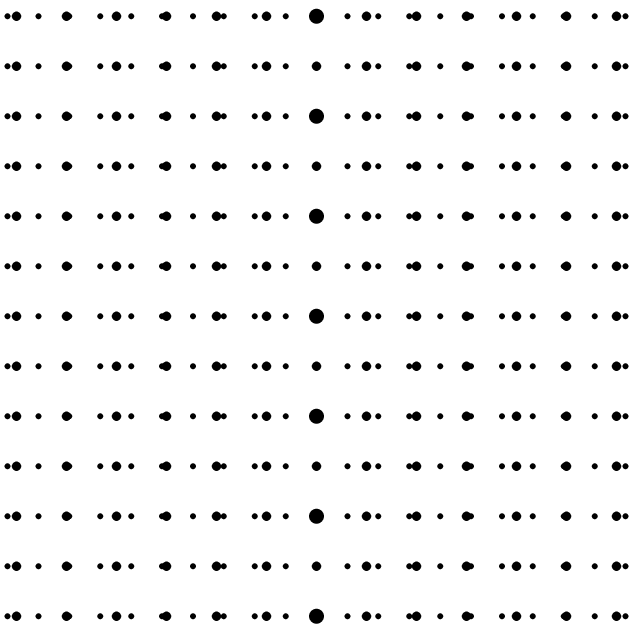
with the dual (reciprocal) lattice . Note that the final term only involves the second components of and , due to the presence of the term in the measure (so only contributes). In the diffraction measure, the composite structure is visible via additional intensities of the peaks along the vertical axis. The total intensity of a Bragg peak at position with is
The corresponding diffraction pattern for the example of Figure 8 is shown in Figure 9.
Of course, this is merely a sketch of any real system. For a more realistic system, one should take into account the modulation in the positions induced by the different local neighbourhoods.128, 131, 119, 132
Here, we consider a simpler case, based on the modulation of a periodic structure. A modulated structure arises by locally displacing positions of a crystalline point set, ensuring a minimal distance between the new positions. For example, start with the integer lattice and deform it by moving the points according to a real-valued displacement function . The deformed point set is then given by
| (6) |
and denotes the corresponding Dirac comb. To be concrete, consider the displacement function , where and are real numbers and where denotes the fractional part of . Since , the deformed point set respects a minimum distance between points, as long as is sufficiently small. Clearly, if is a rational number, the resulting point set is once again periodic, while it is non-periodic for irrational values of , which is the case we are interested in here.
To understand the corresponding set , it is advantageous to use an embedding in the plane, known as the ‘superspace approach’ in crystallography.128 Define a planar lattice as the integer span of two basis vectors
where we use the notation . Consider now the line pattern obtained as the -orbit of the line from the origin to the point (with the end point not included). Then, is the set of intersections of the horizontal axis with these line segments; see Figure 10 for an illustration.

Using the fact that, for irrational , the sequence of numbers is uniformly distributed in the unit interval,85 one can calculate the autocorrelation of the Dirac comb on explicitly. The result is
The corresponding diffraction measure reads
| (7) |
with (complex) amplitudes
| (8) |
where . The map acts on elements of as for any . In this example, is a pure point measure which is supported on a dense set. Despite the denseness of the Bragg peaks, the total intensity scattered into any compact subset of is finite, because the intensities are locally summable. The proof for the diffraction formula is non-trivial. However, this can be interpreted as a special case of the diffraction of model sets (cut and project sets), because the modulated structure (6) is in fact a model set. We now turn our attention to this general notion, and discuss a number of relevant examples and their diffraction.
4.2 Model sets
There are a number of ways to construct aperiodically ordered systems.55 From the viewpoint of diffraction, the best understood is a natural generalisation of lattice-periodic structures obtained by a projection from a higher-dimensional lattice. Such systems are called cut and project sets or model sets,98 and can be produced in a number of essentially equivalent ways,50 including de Bruijn’s grid method41 and Kramer’s ‘Klotz construction’,82 as well as a number of other approaches.99, 66
The model set approach can be viewed as a generalisation of the notion of a quasiperiodic function.31 In the simplest setting, the idea is much like what we saw for the modulated phase in Figure 10 above: The aperiodic structure emerges by taking a cut across a higher-dimensional periodic structure, using a direction that is incommensurate with the lattice. The general setting for the case of Euclidean model sets is encoded in the cut and project scheme (CPS)
| (9) |
where is the physical (sometimes also called direct or parallel) space, and is referred to as the internal (or perpendicular) space. Here, is a lattice in dimensions, and and denote the natural projections onto the physical and internal spaces. It is assumed that is a bijective image of in direct space, and that the set is dense in internal space. As a consequence, the -map98 is well-defined on .
A model set for a given CPS is then a set of the form
| (10) |
where (called the window or acceptance domain) is a relatively compact subset of with non-empty interior. More generally, also translates of such sets are called model sets. The elements of the model set lie in the projected lattice in direct space, and the window in internal space determines which elements of are selected. The conditions on the window ensure that the model set is a Delone set. In fact, a model set is always a Meyer set,96, 98 which means that is uniformly discrete, while is relatively dense. Note that uniform discreteness of implies that of , and is actually a much stronger condition.96, 98, 86, 87
Clearly, the projection approach produces point sets in space rather than the tilings that are conventionally used to model atomic structures of quasicrystals. However, as long as there exists a local rule to switch from the point set to the tiling picture and vice versa, we can consider both structures as equivalent (as any atomic structure will be a local decoration of either), or shortly as MLD (which stands for mutual local derivability).4 For instance, in one dimension, a tiling of by two intervals of different lengths is clearly MLD with the set of left endpoints of all intervals.
In what follows, we only consider regular model sets, so we require that the boundary of the window has zero Lebesgue measure. The Euclidean setting (9) generalises to the case where the internal space is a locally compact Abelian group.96, 98, 115 We shall meet an example later, where the internal space is based on -adic integers.
Regular model sets are pure point diffractive,67, 115, 23 and in this sense are natural generalisations of lattices. This is a central result of the theory of model sets which has been proved by methods of dynamical systems theory,67, 115, 91 in terms of almost periodic measures23, 101, 126 and, following a suggestion by Lagarias, by using the Poisson summation formula for the embedding lattice and Weyl’s lemma on uniform distribution.16 The diffraction measure of the Dirac comb is explicitly given by
| (11) |
Here, is the corresponding Fourier module, which is the projection of the higher-dimensional dual lattice. The amplitudes are given be
| (12) |
where is the characteristic function of the window . Various generalisations, in particular to certain weighted Dirac combs, have been discussed in the literature.115, 23, 16, 111 An alternative (and somewhat complementary) approach based on an average periodic structure can be employed to unravel various modulation features in the diffraction patterns of quasicrystals. This is systematically explained in a recent review136 by Wolny and coworkers; see references cited there for further details.
4.3 One-dimensional examples

We start by re-expressing the modulated point set of Eq. (10) as a cut and project set. To this end, we need to write via an orthogonal projection, rather than via the (implicit) skew projection of Figure 10. This can be done by introducing the matrix and considering the lattice . This lattice and its dual lattice are given in terms of a -basis by
The two generating vectors and the lattice points of are shown in Figure 11.
The set is now a model set for the CPS with lattice (so and both direct and internal space are ). The window is the interval , and the condition selects all lattice points that are located within the shaded strip of Figure 11 (which is the reason why this approach is sometimes also referred to as the strip projection method). For , we get a (non-minimal) embedding of in , and for rational with coprime integers and we obtain a periodic point set with lattice of periods .
The formulas (7) for the diffraction and (8) for the amplitudes now follow from the general result of Eqs. (11) and (12). The Fourier module is , and the action of the -map can be read off from the explicit bases of and given above.
The most frequently invoked example of a one-dimensional (mathematical) quasicrystal is the Fibonacci chain. Its geometric version is built from two intervals (prototiles) and (for long and short) of lengths and . It can be generated by iterating the square of the inflation rule , , starting from a legal seed (such as , where the vertical line indicates the reference point). This leads to the two-sided interval sequence
The bi-infinite sequence is aperiodic, with relative frequencies and for the two prototiles.

Define two point sets and as the left endpoints of the corresponding intervals in the chain, taking the reference point as . They are model sets for the CPS (9) with and
The corresponding planar lattice is
which has density and the dual lattice
One has with the windows
and the -map defined by , so that . The construction is illustrated in Figure 12. The Fibonacci model set is , with window
This way, is a point set of density . Note that it is possible to modify the embedding lattice by scaling the internal space relative to physical space. In particular, multiplying the scale of internal space by , the embedding lattice is a rotated copy of .

The Dirac comb is pure point diffractive, by an application of the model set diffraction theorem67, 115, 23 mentioned before. The diffraction measure is explicitly given by Eq. (11) with the amplitudes
| (13) |
via Eq. (12), where . The phase factor reflects the position of the window, which is centred at . The sum in Eq. (11) runs over the Fourier module
A sketch of the diffraction pattern is shown in Figure 13. Note that the intensity function vanishes if and only if . This means with . Since all such points lie in the Fourier module , we have identified all extinctions. These are a fingerprint of the intrinsic inflation symmetry.
As an example of a limit-periodic structure, consider the period doubling sequence. Written as an element , it is given by , and for . This rule specifies every position except , where we can choose either possibility. Both possibilities can also be obtained as a fixed point sequence of the square of the substitution , . The two sequences have cores
and are locally indistinguishable. They thus define the same system. The underlying Toeplitz structure of a hierarchy of scaled and shifted copies of is apparent from the formula24, 23, 16
for (with added to in the other case). This set can be described as a model set, but with the internal space being the -adic integers. Consequently, the diffraction measure of the Dirac comb is again pure point.
The corresponding diffraction formula can be given explicitly as follows.12, 16 The Fourier module is
so that we can again use Eq. (11). Here, the amplitudes are
with . This parametrisation specifies uniquely. Figure 14 shows the absolute values for . This pattern repeats -periodically.

Further one-dimensional examples will be discussed in Section 5 in the context of continuous diffraction measures. Let us now turn our attention to higher-dimensional model sets.
4.4 Cyclotomic model sets
For the description of two-dimensional tilings, it is advantageous to work with complex numbers in rather than with points in . In , a rotation by an angle just corresponds to multiplication with the complex number . This point of view is a natural generalisation of de Bruijn’s method41 and the Fourier space approach.95 A natural way to implement an -fold rotational symmetry is to choose a primitive th root of unity (so and for ), and to consider the -module of cyclotomic integers, comprising all integer linear combinations of powers of (the solutions of the equation ). One can think of cyclotomic integers as the set of all points in the plane that can be reached by taking steps of unit length along the directions of a regular -star. Clearly, the resulting point set is symmetric under rotations of multiples of ; in fact, under rotations by multiples of if is odd. Therefore, one usually restricts to integers to avoid duplications.
The cases are trivial in the sense that the resulting point sets lie on the real axis. The choices lead to crystallographic point sets, the triangular lattice with sixfold symmetry and the square lattice with fourfold symmetry. Any other choice , , produces a dense point set in the plane, with -fold symmetry for even , and -fold symmetry for odd .
The dense point set can be embedded into a lattice by lifting it to a suitable higher-dimensional space, essentially by making all directions in the -star that are linearly independent over the integers (there are such directions, where is Euler’s totient function) also linearly independent over the real numbers. A natural way to do this is the Minkowski (or Galois) embedding
| (14) |
which defines a lattice . Here, , with , are the Galois automorphisms of the corresponding cyclotomic number field, mapping a primitive root to a primitive root , where , together with a suitable ordering. Note that is the identity map. Using the lattice in a cut and project scheme, with physical space and internal space , we produce cyclotomic model sets, which, for suitably chosen windows, have -fold (-fold) rotational symmetry.
As an explicit example, we consider the classic Ammann-Beenker (or octagonal) tiling2, 28 as a cyclotomic model set with . Other standard examples of this type include the Penrose tiling104 of Figure 2 and the Tübingen triangle tiling19 (both with tenfold symmetry) and Gähler’s shield tiling47, 48 (with twelvefold symmetry). The latter is locally equivalent (MLD) with a tiling introduced by Socolar.120 Since , all these tilings are obtained from cut and project schemes (9) with internal space .

Of course, the resulting tilings are only rotationally symmetric if the window is chosen to have an appropriate rotational symmetry. To obtain the (undecorated) Ammann-Beenker tiling, the window has to be chosen as a regular octagon, of unit edge length. The module
is dense in the plane, and naturally lifts to a hypercubic lattice in four dimensions (the corresponding Minkowski embedding is a scaled and rotated version of ). The -map can be chosen as the Galois automorphism , and the Ammann-Beenker model set is then obtained as
Figure 15 shows the picture in physical and internal space. Selecting points whose -image falls inside the octagonal window (shown on the right of Figure 15) produces the point set in physical space shown on the left. Connecting all points of unit distance (which clearly is a local rule) recovers the Ammann-Beenker tiling, which is MLD with the cyclotomic model set. The decorations needed for the approach via local rules2 add some non-local information, and cannot be recovered from the undecorated tiling alone.120, 48.

The diffraction of the Dirac comb on the Ammann-Beenker model set can be calculated via Eqs. (11) and (12). It is a pure point measure supported on the dual module (with the factor due to the aforementioned scaling of the hypercubic lattice in the Minkowski embedding). The amplitudes (or Fourier-Bohr coefficients) are
because the lattice has density . A central patch of the diffraction image, obtained via an exact calculation of the Fourier transform of the octagonal window, is shown in Figure 16. In principle, the diffraction of any model set can be calculated (at least approximately) in this way, although it may be complicated if the window is not a simple polygon or circle, such as for the square-triangle tilings where the windows have fractal boundaries.18, 63
4.5 Icosahedral model sets
The model set approach works in any dimension. In particular, it can be used to construct icosahedrally symmetric tilings in three-dimensional space, which are particularly relevant for applications in crystallography. The minimum embedding dimension for this purpose is six, because one needs a faithful action of the icosahedral group and an invariant subspace of dimension . In this setting, there exist three different classes of icosahedral model sets, which correspond to the three different hypercubic lattices (primitive, face-centred and body-centred) in six dimensions.116, 112 As body-centred icosahedral structures have not yet been identified in quasicrystals, we concentrate on the other two classes, and discuss one example of either type.
For the primitive icosahedral tiling, we start from a lattice that is similar to the integer lattice , and use a cut and project scheme (9) where both physical and internal space are . The corresponding window is shown in Figure 17; it is a semi-regular polyhedron known as Kepler’s triacontahedron. The triacontahedron has edge length , volume and surface area , where is again the golden ratio. This approach was pioneered by Kramer and Neri,79 and the tiling is also sometimes called the Ammann-Kramer-Neri tiling (Ammann described the tiling earlier by different means, without publishing his findings; compare the corresponding comments in Mackay’s early paper93). Some authors also call it the three-dimensional Penrose tiling, in analogy to the fivefold rhombus tiling in the plane.
The primitive icosahedral tiling is built from two rhombohedral prototiles, a thick (or prolate, called ) and a thin (or oblate, called ) one. They can be defined as the convex hulls of their vertices
where the basis vectors are112
| (15) | ||||||||
These six vectors generate the primitive icosahedral module
which plays the role of in the corresponding cut and project scheme (9). The -map acts as on , where ′ denotes algebraic conjugation (which maps , hence ). In this formulation, the embedding lattice is similar to , and explicitly generated by the -basis with the vectors from Eq. (15). Consequently, the fundamental cell of has volume , so that the density of is .


A sketch of the two prototiles is shown in Figure 18. The rhombohedra have solid angles , and as indicated. The solid angles in both cases add up to . The prototiles have volumes (for ) and (for ). Note that ten rhombohedra of each type can be assembled78, 79 to fill Kepler’s triacontahedron of Figure 17.
Figure 19 shows the only vertex star out of the possible vertex stars of the Kramer-Neri tiling which has full icosahedral symmetry. In any tiling obtained from a generic model set, this vertex type occupies a subset that itself is a model set with the -scaled triacontahedron as its window. This property corresponds to the invariance of the module under multiplication by and reflects the inflation symmetry of the primitive icosahedral tiling. The corresponding (local) inflation rule, however, turns out to be rather complicated and has never been presented in complete detail.

The diffraction of the Dirac comb on the primitive icosahedral model set can be calculated again by Eqs. (11) and (12). The Fourier module in this case is
The diffraction spectrum consists of a dense set of Bragg peaks located on , of which only a discrete subset has intensity above any chosen (positive) threshold. A full calculation of the Fourier transform of the triacontahedron was given by Elser,45 so the intensities can be obtained explicitly.
For simplicity, however, we employ a spherical approximation to the amplitudes, by replacing the triacontahedron by a sphere of equal volume . The radius of the sphere turns out to be
Because the triacontahedral window is well approximated by this sphere, the difference between the approximate and the exact diffraction intensities is tiny, and irrelevant for our purpose. Note that the approximation only affects the values of the amplitudes, not the location of the peaks (except for extinctions, which might show up in the approximation as tiny intensities). The Fourier transform of the spherical window evaluates as
with . Figure 20 shows sections through the corresponding three-dimensional diffraction patterns, orthogonal to the fivefold, threefold and twofold symmetry axes.

An example of an F-type (face-centred) icosahedral model set is Danzer’s tiling,38 which was first constructed from an inflation rule, and is also known as the ABCK tiling, after the labels Danzer used for the four tetrahedral prototiles. In the ABCK tiling, the tetrahedral tiles always occur in the configurations shown in Figure 21, so one can alternatively work with assembled prototiles consisting of four tiles of type A, B or C, and eight tiles of type K.

The ABCK tiling is mutually locally derivable39, 113 from the Socolar-Steinhardt tiling,122 so both describe equivalent structures. An interesting property of Danzer’s ABCK tiling is the fact that it possesses particularly simple perfect local rules, which can be formulated as purely geometric packing rules on the level of the octahedra.38 The Danzer tiling has three icosahedrally symmetric vertex stars, each comprising just one type of tiles, which are shown in Figure 22. Under inflation, these act as seeds of globally icosahedrally symmetric Danzer tilings.

For the Danzer tiling comprising these larger prototiles of Figure 21, all vertices are located on the face-centred icosahedral module
which is a submodule of of index . Explicitly, one has
where . For this choice of coordinates, is not in . The vertex point set can be described as a three-component model set113, 81 based on a cut and project scheme (9) with physical and internal space . The corresponding lattice is the embedding of in , which is similar to the root lattice . The vertices of the four types of (topological) octahedra (thus disregarding their centres) separate into three different types, which stem from different cosets of the embedding lattice.
In fact, the usual description as a three-component model set uses the projections of so-called ‘holes’ in the lattice . Holes are vertices of the Voronoi cells whose distance from points of the lattice is a local maximum.33 If the distance is an absolute maximum, the hole is called deep, otherwise shallow. The vertices of the Danzer tiling then fall into three groups: Vertices of type I are projections from deep holes which lie in the coset , those of type II from deep holes in the coset and vertices of type III from shallow holes in the coset . The corresponding three windows have icosahedral symmetry and are shown in Figure 23. The window for vertex type I is a dodecahedral extension of an icosahedron, with pentagonal edge length and volume , the window for vertex type II is a dodecahedron of edge length and volume , and the third window is a great dodecahedron (a Kepler-Poinsot polyhedron), with pentagonal edge length and volume . The -map is the same as for the primitive model set above.

The diffraction pattern of the Danzer tiling has spots on the corresponding dual module
| (16) |
with as above. Whereas the primitive tilings has diffraction spots on only, the Danzer tiling has additional spots on the shifted copy . Note that the union corresponds to the body-centred icosahedral module.
Due to the relation between the symmetry directions and the shift , not all high-symmetry sections through the origin will show peaks from both modules in Eq. (16). In fact, only the twofold sections through the origin contain peaks from both parts in Eq. (16) and thus display the full Fourier module, while the three- and fivefold sections only contain peaks from . Figure 24 shows the twofold section of the diffraction for a Dirac comb of vertex type II only, so the window is simply a dodecahedron, which we approximate by a sphere of radius . In Figure 24, the ‘black’ diffraction spots belong to , while the grey spots belong to the coset.
To visualise the diffraction along the fivefold axis, we combine the section through the origin with two parallel sections containing the coset reflections. The result is shown in Figure 25. The spots in are again shown in black, while the two different grey colours distinguish the spots in the two parallel planes containing (dark grey) or (light grey). This pattern demonstrates that the overall rotational symmetry here is fivefold (not tenfold) and inversion symmetric. The latter property accounts for the tenfold rotation symmetry of the section through the origin (black spots). Sections with threefold symmetry display the analogous phenomena.

The distinction between the diffraction of a primitive and of a face-centred icosahedral model set is thus immediately recognisable from the spot locations in a twofold section. For further (practical) details and examples we refer to the recent literature.125

Within the realm of regular model sets, diffraction is thus pretty well understood. We know that regular model sets are pure point diffractive,67, 115, 23 and Eqs. (11) and (12) provide explicit expressions for the intensities in terms of the Fourier transform of the window. Homometry of model sets (within the same cut and project scheme) can be traced back to equality of the covariogram of the window, and explicit examples of homometric model sets have been constructed.9 Thermal fluctuations can be taken into account in a fashion that is analogous to the crystallographic case;68, 6 see Section 5.3 below.
The Bragg diffraction has some robustness property beyond the class of regular model sets. Recently, Strungaru126 proved that, for any Meyer set , the corresponding Dirac comb always shows a non-trivial point diffraction, though in general the spectrum will be mixed and not pure point. However, the point part is substantial in the sense that for any , the set of peaks (all peaks with intensity near the maximum intensity) is relatively dense. While we do not have a complete answer to the question what structures are pure point diffractive,32 it is clear that a pure point spectrum imposes strong constraints on the possible structures.20
For the remainder of this article, we are looking at systems that show continuous diffraction, both singular and absolutely continuous. The discussion of examples with and without random disorder will shed some light on the much more complex situation beyond the pure point diffractive regime.
5 Systems with continuous diffraction
It seems a relatively recent experimental observation that diffuse scattering (as an indication of structural disorder, and not just of thermal fluctuations) is a widespread phenomenon.133, 135 It is thus natural to also investigate continuous diffraction spectra from a more mathematical perspective. Again, we briefly present illustrative examples, most of which have been analysed completely and rigorously by now.
5.1 Singular continuous diffraction
Let us begin by recalling the paradigm of singular continuous diffraction, the Thue-Morse (or Pruhet-Thue-Morse) system.1 It is usually defined via the substitution rule , . A bi-infinite fixed point sequence emerges from iterating the square of this rule with the legal seed . Define the Dirac comb
where and . One can now show that the autocorrelation measure exists134, 94, 73, 10 and is of the form
with and the recursion
which is valid for all . This exact renormalisation-type structure is the golden key to prove the spectral type and to calculate the measure explicitly.

The diffraction measure is -periodic,5, 8 and hence of the form with a positive, singular continuous measure . To describe the latter explicitly, one defines the distribution function on the unit interval. It is consistently extended to a function on by setting for . This way, is -periodic and possesses the uniformly converging Fourier series
For computational purposes, however, it is advantageous to use an approximation in terms of a uniformly converging sequence of distribution functions as follows. Define and the functional iteration
for . Since this iteration maps distribution functions for absolutely continuous measures to distribution functions of the same type, one can write with a Radon-Nikodym density . One can now check explicitly that this leads to
where the empty product is to be evaluated as . Since the densities become increasingly spiky (and do not converge as a sequence of functions), one uses the distribution functions to illustrate the resulting measure. Note that the sequence converges uniformly,8 but not absolutely. This is in line with the fact that is singular continuous, and thus cannot be approximated by a norm-converging sequence of absolutely continuous measures.108 The resulting limit distribution function is illustrated in Figure 26. Despite its similarity with the Cantor measure of Figure 5, is a strictly increasing function. This means that there is no proper plateau here.
A non-trivial planar example emerges from the squiral inflation rule from Figure 10.1.4 in Grünbaum and Shephard.56 It effectively leads to an aperiodic -colouring of the square lattice, according to the chirality of the square dissections; see Figure 27 for an illustration. Positioning a point measure of weight or in the centre of the two types of squares, one obtains a weighted Dirac comb with average weight . Due to the inflation structure, one can derive a recursion formula for the corresponding autocorrelation.15, 16

By constructive methods, in complete analogy to the case of the Thue-Morse sequence, one can show that this Dirac comb leads to a purely singular continuous diffraction measure.15, 16 As in the one-dimensional case, it can explicitly be calculated, and represented as a two-dimensional Riesz product. The result reads
| (17) |
where the function is defined by
As in the one-dimensional case, the corresponding distribution function possesses a uniformly convergent Fourier series representation, which involves the autocorrelation coefficients. The density function (bottom) and the corresponding distribution function (top, normalised such that ) are shown in Figure 28.


5.2 Rudin-Shapiro chain and its Bernoullisation
A simple, deterministic system with continuous diffraction is the binary Rudin-Shapiro chain. While it is usually presented via a four-letter substitution rule, the corresponding weighted Dirac comb can be defined by the sequence of weights with , initial conditions , , and the recursion
| (18) |
The arrangement of the two weights looks as follows
![[Uncaptioned image]](1205.3633v1/rschain.png) |
where the line denotes the origin, and filled (open) dots correspond to weights ().
Despite the deterministic structure, the autocorrelation measure of the balanced Dirac comb (which has average scattering strength ) can be shown114, 117, 105 to be . A simple proof of this is obtained by considering the induced recursion relation for the autocorrelation coefficients.11, 13 The corresponding diffraction measure is thus , which is purely absolutely continuous, and shows no trace whatsoever of the underlying deterministic order in the sequence. In fact, the system is (almost surely, meaning for almost all realisations of the random sequence) homometric with the random Dirac comb on with weights from chosen at random, independently at each position and with equal probability.
We can combine the deterministic sequence and independently chosen random numbers by considering the Bernoullisation of the Dirac comb , which we define as11
| (19) |
Here, is the binary Rudin-Shapiro sequence of weights from Eq. (18), whereas is an i.i.d. family of random numbers, each taking values and with probabilities and (so ), respectively. The limit cases bring us back to the deterministic Dirac comb , while the case corresponds to the Bernoulli comb with weights and mentioned above. The Bernoullisation thus interpolates between the deterministic Rudin-Shapiro sequence and the completely uncorrelated sequence of independent random numbers. It can also be interpreted as a ‘model of second thoughts’, where the sign of the weight at position is changed with probability .
Using the strong law of large numbers,46 it can be shown11, 16 that the autocorrelation of the Dirac comb is almost surely given by
irrespective of the value of the parameter . So the diffraction of this Dirac comb, for any choice of the parameter , is (almost surely) , and the entire family of Dirac combs is homometric.
This simple example highlights the fact that diffraction in general cannot distinguish ‘order’ in the sense of a deterministic structure from that in the presence of entropy. Note that the deterministic Rudin-Shapiro sequence has zero entropy, while the Bernoulli comb has entropy , which is the maximum entropy for a binary sequence. For general , the entropy is , so it varies continuously between and . Regardless, the diffraction of all these combs is the same. This result provides a glimpse at how degenerate, and hence difficult, the inverse problem can be in the presence of continuous spectra. Similar arguments can be used in higher dimensions (in particular by considering product structures), and examples in two dimensions involving lower rank entropy have also been discussed.27, 14
5.3 Random displacements and thermal fluctuations
There are various important applications of Bernoulli-type disorder in real systems. The most obvious one is known as the random occupation model, which covers lattice gases and models of chemical disorder. Traditionally, this has been formulated for lattice-based systems only,35, 130 but the corresponding results hold in much greater generality. This includes model sets,21 but also structures with a substantial degree of positional disorder.83, 84, 6 It turns out that the lattice assumption can be replaced by rather general principles from probability theory that revolve around the strong law of large numbers.46
This change of perspective is also of value for the treatment of the effects of thermal fluctuations to the diffraction of solids. In fact, rather than restricting to a lattice and small vibrations in a harmonic potential, the famous Debye-Waller contribution35 can alternatively be derived from the assumption that the scatterers are randomly displaced from their equilibrium positions, independently of each other, but based on the same probability distribution. This opens the door to another application of the strong law of large numbers, as was first observed by Hof.68 Two further advantages are the validity for considerably more general point sets than lattices and the independence of the argument of the small displacement assumption. At least for sufficiently high temperatures, this alternative approach is reasonable.
Consider a Delone set that is sufficiently nice (where we refer to the literature68, 6 for the precise conditions). In particular, we assume that the Dirac comb possesses the autocorrelation . The random displacement is described as
where is a family of i.i.d. random translation vectors with common probability distribution . Then, with probability one, has the autocorrelation
| (20) |
The corresponding diffraction is obtained by Fourier transform and reads
| (21) |
Here, is a uniformly continuous function on that vanishes at infinity, and the formula holds almost surely, as Eq. (20). If , the diffraction of , is a pure point measure, the pure point part of is given by (hence by a modulation of the intensities, which is the Debye-Waller factor), while the continuous part is . Note, however, that Eq. (21) is by no means restricted to pure point diffractive systems. An explicit dependence on the temperature can be modelled by the appropriate choice of the displacement distribution . Further details and generalisations are discussed in the literature.83, 6
5.4 Random tilings
Random tilings form a particularly interesting and relevant class of structures, as was early pointed out by Elser.44 The structure of the various ensembles and their diffraction is not as well understood as in the deterministic case, though a fairly complete picture was sketched by Henley.62 From a physical point of view, most results are ‘clear’, on the basis of convincing (scaling) arguments from statistical mechanics. The mathematical counterpart, however, is still incomplete, and various properties have escaped a proof so far, particularly in dimensions and higher. In fact, it is a characteristic feature of random tilings to show a strong dependence on the dimension, as we will illustrate by some examples.
Let us first consider a random version of the Fibonacci chain. Here, one starts with two prototiles as before (one interval of length and one of length ), and builds a tiling of by choosing them with probabilities and , where leads (almost surely) to realisations with the same relative tile frequencies as the deterministic chain of Figure 12. Due to the linear arrangement, the ensemble is well under control by elementary methods from probability theory. In particular, one can either invoke the ergodicity of the Bernoulli (coin tossing) chain17 or the renewal theorem6 to show that the random Dirac comb obtained this way almost surely leads to the diffraction measure
| (22) |
with the Radon-Nikodym density function
The factor is the density of the corresponding point set, which equals that of the deterministic counterpart discussed earlier. Apart from the trivial Bragg peak at , the diffraction is thus absolutely continuous. Figure 29 shows the function , which is smooth but still shows a spiky structure that resembles the pure point diffraction of the perfectly ordered Fibonacci chain from Figure 13 to an amazing degree.

The mechanism behind the absolutely continuous nature of the diffraction in Eq. (22) can be understood as follows. Due to the choice of the intervals, each realisation can be lifted within the cut and project scheme of the perfect Fibonacci chain of Figure 12. Almost surely, one then obtains a sequence of lattice points that deviate from the perfect case via fluctuations that diverge linearly with the system size.62, 64 This destroys the coherence needed for Bragg peaks (at ) or singular continuous contributions to .
Random tilings in the plane show a different behaviour, which also depends on the symmetry. In particular, it is important whether one deals with a crystallographic symmetry (such as statistical three- or sixfold symmetry in the lozenge tiling) or not (such as statistical eightfold symmetry in the random octagonal tiling). An example of the former case, with broken symmetry, is illustrated in Figure 30. The underlying ensemble is well studied in statistical physics.74, 43, 76, 64, 77
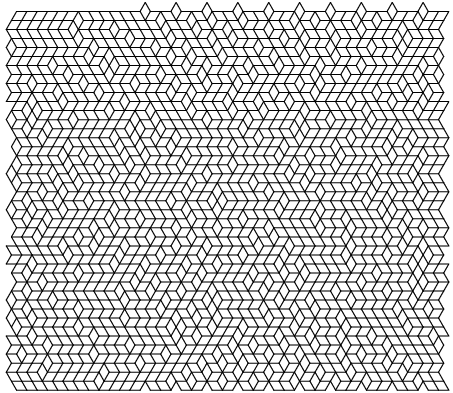
The lozenge (or rhombus) with opening angle occurs in three possible orientations in all typical lozenge random tilings (which are subject to the condition that any resulting tiling is face to face and covers the plane without overlaps). One can now use the relative frequencies of the three prototiles to parametrise the ensemble. By purely group theoretic methods, one can then show that the entropy has a unique maximum at the (unique) point of maximal symmetry.110, 62 This shows an interesting entropic mechanism for the stabilisation of tilings with statistical symmetry. The value of the entropy (calculated per tile) is known exactly from a mapping to the two-dimensional antiferromagnetic Ising model on the triangular lattice, which was exactly solved by Wannier.129
The underlying ensemble is special also in the sense that one does not only know the free energy and the entropy, but also the two-point correlation functions, at least asymptotically. Since this is the autocorrelation of the system, when placing point scatterers of unit mass on each vertex point, the diffraction measure for almost all realisations of the lozenge random tiling (with edge length , say) is of mixed type, and has the form . The pure point part is17
| (23) |
where is the dual lattice of the triangular lattice, spanned by and , and is a shorthand for the wave vector . The pure point part reflects the underlying lattice structure,5 while the absolutely continuous one is the fingerprint of the structural disorder. It is effectively repulsive in nature, as expected, which manifests itself17, 26 in the property that the diffuse intensity is ‘repelled’ by the Bragg peaks.


The diffraction of the example from Figure 30 is shown in Figure 31. The pattern is lattice periodic. The pure point part (big spots) follows from the exact formula in (23), while the continuous part (small spots) was calculated numerically by Höffe17, 64 via FFT techniques.
The corresponding situation for the randomised Ammann-Beenker or octagonal tiling looks similar at first sight, and leads (via simpleton flip thermalisation, see Figure 32) to patches of the form shown in Figure 33. However, the possible vertex positions are no longer restricted to a lattice, but only to the module with a primitive th root of unity. This module is the corresponding set of cyclotomic integers and a dense point set in the plane, as explained earlier. As a result, apart from the trivial Bragg peak at , the diffraction measure will be continuous, with singular and absolutely continuous components. The reason behind this is the logarithmically diverging fluctuation of the embedding surface from the deterministic surface of the model set relative.62 Due to the larger positional freedom of the vertex points, this fluctuation is strong enough to destroy the coherence that is needed for non-trivial Bragg peaks, but not strong enough to avoid singular continuous contributions.64

Unfortunately, this is one of the claims that have not yet been proved, though there can be hardly any doubt about its correctness. A numerical calculation16 of the diffraction of the finite patch shown in Figure 33 leads to the pattern of Figure 34, a similar result was obtained by Höffe64 via FFT. A comparison with the diffraction of the perfect Ammann-Beenker tiling in Figure 16 still reveals a lot of similarities, despite the approximative nature of the calculation. In particular, one can clearly map the strong peaks of the perfect case to positions of the random tiling diffraction, and also various ring-type structures are clearly common to both images. In view of these similarities, it is not clear to what extent kinematic diffraction of a finite patch can distinguish the perfect from a random tiling.
The simpleton flip of Figure 32 provides a standard approach for the preparation of random tiling samples. It works well also for other tilings with rhombic prototiles, where one might have different types of simpletons to consider (for instance, there are two such configurations in the rhombic Penrose tiling). One usually starts from a periodic approximant (to minimise boundary effects) to a perfect tiling, which is not difficult to construct, and runs the simpleton flip thermalisation until correlations have decayed. In such ensembles, the process can be shown to be topologically transitive, so that the entire ensemble compatible with these boundary conditions is accessible.62, 64 Note, however, that there are other important ensembles, such as the random square triangle tilings, where no such local flip exists. Here, one needs alternative methods, such as the well-studied ‘zipper’ move102 that temporarily introduces some new (auxiliary) tiles that enable a randomisation path, until the created tiles annihilate themselves again and leave a modified square triangle tiling behind.

Finally, the case of random tilings in -space is clearly of great interest. A natural candidate from the very beginning44, 62 has been the randomised version of the primitive icosahedral tiling, which is built from the two rhombohedra of Figure 18. While there are complete vertex configurations in the Kramer-Neri projection tiling, counted up to icosahedral isometries, there are possible ones in a typical random tiling.30 So, it is clear that this version locally shows a much higher degree of disorder. However, unlike the previous examples, the fluctuations away from the embedding hypersurface seem to be bounded,44, 62 which implies a diffraction of mixed type, this time with a pure point and an absolutely continuous component — despite the statistical icosahedral symmetry, which is non-crystallographic; a numerical confirmation was obtained by Monte-Carlo simulation techniques.127
If one employs a statistical variant of the projection method, the fluctuations mentioned above lead to a distribution in internal space that can be described by a density function. The latter will resemble a Gaussian profile,44, 62 which makes the pure point part of the diffraction explicitly accessible via an appropriate extension of the model set theorem to this case.111 This gives diffraction formulas of PSF type where the sums on both sides run over dense point sets. A further generalisation was recently formulated for measures by Lenz and Richard.90
6 Outlook
The discovery of quasicrystals118 in 1982 had a profound impact on various disciplines, including mathematics and, in particular, to harmonic analysis and mathematical diffraction theory. The approach described above emerged from the investigation of aperiodically ordered systems, and offers a method that can be applied to a wide range of structures.
After 30 years of quasicrystal research, the diffraction of mathematical quasicrystals that are described by cut and project sets (regular model sets) is well understood. Such structures are pure point diffractive, much as conventional crystals, except that the Bragg peaks are supported on a point set that is dense in space. For many standard examples, the corresponding diffraction amplitudes can be calculated explicitly, for instance in terms of Fourier transforms of the corresponding window(s).
The situation changes quickly if one leaves the realm of model sets. As discussed, Meyer sets still inherit some of the structure, in the sense that their diffraction measure contains non-trivial pure point components. For substitution (or inflation) based structures, examples with all spectral types are known. In this article, we met examples of all three types — the Fibonacci chain (which is a pure point diffractive model set), the Thue-Morse chain (which has singular continuous diffraction) and the Rudin-Shapiro chain (with absolutely continuous spectrum). In fact, it is easy to come up with a substitution system that has a mixed spectrum comprising all three spectral types.
Quasicrystals are expected to contain some inherent (or structural) disorder, and it is therefore desirable to understand the effect of disorder on diffraction, and, vice versa, the conclusions on disorder that one can draw from examining diffraction patterns, in particular with regard to continuous diffraction. This is far from being well understood, but the examples discussed above provide a glimpse at the general situation. As the Bernoullisation example shows, diffraction cannot always detect the nature of ‘order’, for instance whether the latter is of deterministic or entropic origin. Conversely, diffuse diffraction does not always need to be a sign of random disorder. At present, we only have a very limited knowledge of how large the homometry classes can be. In the pure point diffractive case, a recent approach by Lenz and Moody88, 89 provides one possibility for an abstract parametrisation. Unfortunately, this approach does not seem to be extendable to cover continuous diffraction components. The investigation of further examples with different types or degrees of order will hopefully shed more light on this matter.
One does not have to go far to find examples of important, yet still not completely understood systems. A prominent one is the Conway-Radin pinwheel tiling.106 This tiling is based on a single triangular prototile (of edge lengths , and ), with an inflation rule of linear inflation multiplier , so each re-scaled triangle (which is planar) is dissected into five congruent copies. Figure 35 shows a photograph of a patch of the tiling, which has been used as a theme for Melbourne’s Federation Square development. Because the inflation contains a rotation that is incommensurate with , a new direction is introduced in each inflation step. Consequently, each infinite pinwheel tiling contains triangles in infinitely many distinct orientations, and the corresponding tiling space even has complete circular symmetry.106, 107, 100 The diffraction patterns shows striking similarity to a powder diffraction from a square-lattice based structure.7 While there is strong evidence for sharp rings in the diffraction pattern (which are singularly continuous in the plane), mimicking the case of the rotation-averaged square-lattice structure, the presence of further rings or absolutely continuous components is still unclear.

More generally, one needs a unified setting for the diffraction of systems with mixed spectra. An interesting suggestion was made by Gouéré53 on the basis of the intensity measure of the Palm measure of a point process. This provides an alternative way to define the autocorrelation of the system. It is possible to include cases such as crystallographic systems or model sets into this scheme,88, 89 and it was recently also shown6 how to use this approach in a systematic way for systems with various kinds of disorder. Since the theory of point processes is a highly developed branch36, 37 of modern probability theory, the use of these methods looks rather promising.
Acknowledgements
It is our pleasure to thank Franz Gähler and Peter Zeiner for comments and discussions. This work was supported by the German Research Council (DFG), within the CRC 701.
References
- 1 J.-P. Allouche and J. Shallit. Automatic Sequences: Theory, Applications, Generalizations, Cambridge University Press, Cambridge, 2003.
- 2 R. Ammann, B. Grünbaum and G.C. Shephard, Aperiodic tiles, Discr. Comput. Geom., 1992, 8, 1–25.
- 3 F. Axel and D. Gratias (eds.), Beyond Quasicrystals, Springer, Berlin and Les Editions de Physique, Les Ulis, 1995.
- 4 M. Baake, A guide to mathematical quasicrystals, in: Quasicrystals – An Introduction to Structure, Physical Properties and Applications, eds. J.-B. Suck, M. Schreiber and P. Häussler, Springer, Berlin, 2002, pp. 17–48; arXiv:math-ph/9901014.
- 5 M. Baake, Diffraction of weighted lattice subsets, Can. Math. Bulletin, 2002, 45, 483–498; arXiv:math.MG/0106111.
- 6 M. Baake, M. Birkner and R.V. Moody, Diffraction of stochastic point sets: Explicitly computable examples, Commun. Math. Phys., 2010, 293, 611–660; arXiv:0803.1266.
- 7 M. Baake, D. Frettlöh and U. Grimm, A radial analogue of Poisson’s summation formula with applications to powder diffraction and pinwheel patterns, J. Geom. Phys., 2007, 57, 1331–1343; arXiv:math/0610408.
- 8 M. Baake, F. Gähler and U. Grimm, Spectral and topological properties of a family of generalised Thue-Morse sequences, J. Math. Phys., 2012, 53, 032701; arXiv:1201.1423.
- 9 M. Baake and U. Grimm, Homometric model sets and window covariograms, Z. Krist., 2007, 222, 54–58; arXiv:math.MG/0610411.
- 10 M. Baake and U. Grimm, The singular continuous diffraction measure of the Thue-Morse chain, J. Phys. A.: Math. Theor., 2008, 41, 422001; arXiv:0809.0580.
- 11 M. Baake and U. Grimm, Kinematic diffraction is insufficient to distinguish order from disorder, Phys. Rev. B, 2009, 79, 020203(R) and 2009. 80, 029903(E); arXiv:0810.5750.
- 12 M. Baake and U. Grimm, Diffraction of limit periodic point sets, Philos. Mag., 2011, 91, 2661–2670; arXiv:1007.0707.
- 13 M. Baake and U. Grimm, Kinematic diffraction from a mathematical viewpoint, Z. Krist., 2011, 226, 711–725; arXiv:1105.0095.
- 14 M. Baake and U. Grimm, A comment on the relation between diffraction and entropy, Entropy, 2012, 14, 856–864; arXiv:1205.0392.
- 15 M. Baake and U. Grimm, Squirals and beyond: Substitution tilings with singular continuous spectrum, preprint arXiv:1205.1384.
- 16 M. Baake and U. Grimm, Theory of Aperiodic Order: A Mathematical Invitation, Cambridge University Press, Cambridge, in preparation.
- 17 M. Baake and M. Höffe, Diffraction of random tilings: some rigorous results, J. Stat. Phys., 2000, 99, 219–261; arXiv:math-ph/9904005.
- 18 M. Baake, R. Klitzing and M. Schlottmann, Fractally shaped acceptance domains of quasiperiodic square-triangle tilings with dodecagonal symmetry, Physica A, 1992, 191, 554–558.
- 19 M. Baake, P. Kramer, M. Schlottmann and D. Zeidler, Planar patterns with fivefold symmetry as sections of periodic structures in -space, Int. J. Mod. Phys. B, 1990, 4, 2217–2268.
- 20 M. Baake, D. Lenz and C. Richard, Pure point diffraction implies zero entropy for Delone sets with uniform cluster frequencies, Lett. Math. Phys., 1997, 82, 61–77; arXiv:0706.1677.
- 21 M. Baake and R.V. Moody, Diffractive point sets with entropy, J. Phys. A: Math. Gen., 1998, 31, 9023–9039; arXiv:math-ph/9809002.
- 22 M. Baake and R.V. Moody (eds.), Directions in Mathematical Quasicrystals, CRM Monograph Series, vol. 13, AMS, Providence, RI, 2000.
- 23 M. Baake and R.V. Moody, Weighted Dirac combs with pure point diffraction, J. reine angew. Math. (Crelle), 2004, 573, 61–94; arXiv:math.MG/0203030.
- 24 M. Baake, R.V. Moody and M. Schlottmann, Limit-(quasi)periodic point sets as quasicrystals with -adic internal spaces, J. Phys. A: Math. Gen., 1998, 31, 5755–5765; arXiv:math-ph/9901008.
- 25 M. Baake, M. Schlottmann and P.D. Jarvis, Quasiperiodic patterns with tenfold symmetry and equivalence with respect to local derivability, J. Phys. A: Math. Gen., 1991, 24, 4637–4654.
- 26 M. Baake and B. Sing, Diffraction spectrum of lattice gas models above , Lett. Math. Phys., 2004, 68, 165–173; arXiv:math-ph/0405064.
- 27 M. Baake and T. Ward, Planar dynamical systems with pure Lebesgue diffraction spectrum, J. Stat. Phys., 2010, 140, 90–102; arXiv:1003.1536.
- 28 F.P.M. Beenker, Algebraic theory of non-periodic tilings of the plane by two simple building blocks: A square and a rhombus, TH-Report 82-WSK-04, TU Eindhoven, 1982.
- 29 C. Berg and G. Forst, Potential Theory on Locally Compact Abelian Groups, Springer, Berlin, 1975.
- 30 S.I. Ben-Abraham, M. Baake, P. Kramer and M. Schlottmann, Regular and defective vertex configuration in icosahedral structures, J. Non-Cryst. Solids, 1993, 153–154, 132–136.
- 31 H. Bohr, Almost Periodic Functions, Chelsea, New York, reprint, 1947.
- 32 E. Bombieri and J.E. Taylor, Which distributions diffract? An initial investigation, J. Phys. Colloque, 1986, 47, 19–28.
- 33 J.H. Conway and N.J.A. Sloane, Sphere Packings, Lattices and Groups, Springer, New York, 3rd edn, 1999.
- 34 A. Córdoba, Dirac combs, Lett. Math. Phys., 1989, 17, 191–196.
- 35 J.M. Cowley, Diffraction Physics, North-Holland, Amsterdam, 3rd edn, 1995.
- 36 D.D. Daley and D. Vere-Jones, An Introduction to the Theory of Point Processes I: Elementary Theory and Methods, Springer, New York, 2nd edn, 2nd corr. printing, 2005.
- 37 D.D. Daley and D. Vere-Jones, An Introduction to the Theory of Point Processes II: General Theory and Structure, Springer, New York, 2nd edn, 2008.
- 38 L. Danzer, Three-dimensional analogs of the planar Penrose tilings and quasicrystals, Discr. Math., 1989, 76, 1–7.
- 39 L. Danzer, Z. Papadopolos and A. Talis, Full equivalence between Socolar’s tilings and the (A,B,C,K)-tilings leading to a rather natural decoration, Int. J. Mod. Phys. B, 1993, 7, 1379–1386.
- 40 M. de Boissieu, Study of the structure and physical properties of quasicrystals using large scale facilities, Comptes Rendus Physique, 2012, 13, 207–217.
- 41 N.G. de Bruijn, Algebraic theory of Penrose’s non-periodic tilings of the plane. I & II, Kon. Nederl. Akad. Wetensch. Proc. Ser. A, 1981, 84, 39–52 and 53–66.
- 42 P.M. de Wolff, The pseudo-symmetry of modulated crystal structures, Acta Cryst. A, 1974, 30, 777–785.
- 43 C. Domb and M.S. Green (eds.), Phase Transitions and Critical Phenomena. Vol. 1. Exact Results, Academic Press, London, 1972.
- 44 V. Elser, Comment on “Quasicrystals: A new class of ordered structures”, Phys. Rev. Lett., 1985, 54, 1730.
- 45 V. Elser, The diffraction pattern of projected structures, Acta Cryst. A, 1986, 42, 36–43.
- 46 N. Etemadi, An elementary proof of the strong law of large numbers, Z. Wahrscheinlichkeitsth. verw. Gebiete, 1981, 55, 119–122.
- 47 F. Gähler, Quasicrystal Structures from the Crystallograhic Viewpoint, PhD thesis no. 8414, ETH Zürich, 1988.
- 48 F. Gähler, Matching rules for quasicrystals: The composition-decomposition method, J. Non-Cryst. Solids, 1993, 153–154, 160–164.
- 49 F. Gähler, P. Gummelt and S.I. Ben-Abraham, Generation of quasiperiodic order by maximal cluster covering, in Kramer and Papadopolos,80 pp. 63–95.
- 50 F. Gähler and J. Rhyner, Equivalence of the generalised grid and projection methods for the construction of quasiperiodic tilings, J. Phys. A: Math. Gen., 1986, 19, 267–277.
- 51 J. Gil de Lamadrid and L.N. Argabright, Almost periodic measures, Memoirs AMS, 1990, 65, no. 428.
- 52 C. Goodman-Strauss, Matching rules and substitution tilings, Ann. Math., 1998, 147, 181–223.
- 53 J.-B. Gouéré, Diffraction and Palm measure of point processes, C. R. Acad. Sci. (Paris), 2003, 342, 141–146; arXiv:math.PR/0208064.
- 54 U. Grimm and M. Baake, Homometric point sets and inverse problems, Z. Krist., 2008, 223, 777–781; arXiv:0808.0094.
- 55 U. Grimm and M. Schreiber, Aperiodic tilings on the computer, in: Quasicrystals: An Introduction to Structure, Physical Properties, and Applications, eds. J.-B. Suck, M. Schreiber and P. Häussler, Springer, Berlin, 2002, pp. 49–66; arXiv:cond-mat/9903010.
- 56 B. Grünbaum and G.C. Shephard, Tilings and Patterns, Freeman, New York, 1987,
- 57 F.A. Grünbaum and C.C. Moore, The use of higher-order invariants in the determination of generalized Patterson cyclotomic sets, Acta Cryst. A, 1995, 51, 310–323.
- 58 P. Gummelt, Penrose tilings as coverings of congruent decagons, Geom. Dedicata, 1996, 62, 1–17.
- 59 P. Gummelt, Aperiodische Überdeckungen mit einem Clustertyp, Shaker, Aachen, 1999.
- 60 E. Harris and D. Frettlöh, Tilings Encyclopedia, http://tilings.math.uni-bielefeld.de/.
- 61 C. L. Henley, Cluster maximization, non-locality, and random tilings, in: Proccedings of the 6th International Conference on Quasicrystals, eds. S. Takeuchi and T. Fujiwara, World Scientific, Singapore, 1998, pp. 27–30.
- 62 C.L. Henley, Random tiling models, in: Quasicrystals: The State of the Art, eds. D. P. DiVincenzo and P. J. Steinhardt, World Scientific, Singapore, 1999, 2nd edn, pp. 459–560.
- 63 J. Hermisson, C. Richard and M. Baake, A guide to the symmetry structure of quasiperiodic tiling classes, J. Phys. I France, 1997, 7, 1003–1018; mp_arc/02-180.
- 64 M. Höffe, Diffraktionstheorie stochastischer Parkettierungen, Shaker, Aachen, 2001.
- 65 M. Höffe and M. Baake, Surprises in diffuse scattering, Z. Krist., 2000, 215, 441–444; arXiv:math-ph/0004022.
- 66 C. Hohneker, P. Kramer, Z. Papadopolos and R.V. Moody, Canonical icosahedral quasilattices for the -phase generated by coherent phases in physical space, J. Phys. A: Math. Gen., 1997, 30, 6493–6507.
- 67 A. Hof, On diffraction by aperiodic structures, Commun. Math. Phys., 1995, 169, 25–43.
- 68 A. Hof, Diffraction by aperiodic structures at high temperatures, J. Phys. A: Math. Gen., 1995, 28, 57–62.
- 69 A. Hof, Diffraction by aperiodic structures, in: Moody,97 pp. 239–268.
- 70 T. Ishimasa, H.-U. Nissen and Y. Fukano, New ordered state between crystalline and amorphous in Ni-Cr particles, Phys. Rev. Lett., 1985, 55, 511–513.
- 71 A. Janner and T. Janssen, Symmetry of periodically distorted crystals, Phys. Rev. B, 1977, 15, 643–658.
- 72 H.-C. Jeong and P.J. Steinhardt, Cluster approach for quasicrystals, Phys. Rev. Lett., 1994, 73, 1943–1946.
- 73 S. Kakutani, Strictly ergodic symbolic dynamical systems, in: Proc. 6th Berkeley Symposium on Math. Statistics and Probability, eds. L. M. LeCam, J. Neyman and E. L. Scott, Univ. of California Press, Berkeley, 1972, pp. 319–326.
- 74 P.W. Kasteleyn, Dimer statistics and phase transitions, J. Math. Phys., 1963, 4, 287–293.
- 75 A. Katz, Matching rules and quasiperiodicity: the octagonal tilings, in: Axel and Gratias,3 pp. 141–189.
- 76 R. Kenyon, Local statistics of lattice dimers, Ann. Inst. H. Poincaré B, 1997, 33, 591–618; arXiv:math.CO/0105054.
- 77 R. Kenyon, The planar dimer model with boundary: A survey, in: Baake and Moody,22 pp. 307–328.
- 78 G. Kowalewski, Der Keplersche Körper und andere Bauspiele, Koehlers Antiquarium, Leipzig, 1938.
- 79 P. Kramer and R. Neri, On periodic and non-periodic space fillings of obtained by projection, Acta Cryst. A, 1984, 40, 580–587; Erratum, Acta Cryst. A, 1985, 41, 619.
- 80 P. Kramer and Z. Papadopolos, Coverings of Discrete Quasiperiodic Sets, Springer, Berlin, 2003.
- 81 P. Kramer, Z. Papadopolos, M. Schlottmann and D. Zeidler, Projection of the Danzer tiling, J. Phys. A: Math. Gen., 2003, 27, 4505–4517.
- 82 P. Kramer and M. Schlottmann, Dualisation of Voronoi domains and Klotz construction: A general method for the generation of proper space fillings, J. Phys. A: Math. Gen., 1989, 22, L1097–L1102.
- 83 C. Külske, Universal bounds on the selfaveraging of random diffraction measures, Probab. Th. Relat. Fields, 2003, 126, 29–50; arXiv:math-ph/0109005.
- 84 C. Külske, Concentration inequalities for functions of Gibbs fields with application to diffraction and random Gibbs measures, Commun. Math. Phys., 2003, 239, 29–51.
- 85 L. Kuipers and H. Niederreiter, Uniform Distribution of Sequences, Dover, New York, reprint, 2006.
- 86 J.C. Lagarias, Meyer’s concept of quasicrystal and quasiregular sets, Commun. Math. Phys.,1996, 179, 365–376.
- 87 J.C. Lagarias, Geometric models for quasicrystals I. Delone sets of finite type, Discr. Comput. Geom., 1999, 21, 161–191.
- 88 D. Lenz and R.V. Moody, Extinctions and correlations for uniformly discrete point processes with pure point dynamical spectra, Commun. Math. Phys., 2009, 289, 907–923; arXiv:0902.0567.
- 89 D. Lenz and R.V. Moody, Stationary processes with pure point diffraction, Preprint, arXiv:1111.3617.
- 90 D. Lenz and C. Richard, Pure point diffraction and cut and project schemes for measures: The smooth case, Math. Z., 2007, 256, 347–378; arXiv:math.DS/0603453.
- 91 D. Lenz and N. Strungaru, Pure point spectrum for measure dynamical systems on locally compact Abelian groups, J. Math. Pures Appl., 2009, 92, 323–341; arXiv:0704.2498.
- 92 D. Levine and P.J. Steinhardt, Quasicrystals: A new class of ordered structures, Phys. Rev. Lett., 1984, 53, 2477–2480.
- 93 A.L. Mackay, De nive quinquangula: On the pentagonal snowflake, Sov. Phys. Cryst., 1981, 26, 517–522.
- 94 K. Mahler, The spectrum of an array and its application to the study of the translation properties of a simple class of arithmetical functions. Part II: On the translation properties of a simple class of arithmetical functions, J. Math. Massachusetts, 1927, 6, 158–163.
- 95 N.D. Mermin, D.S. Rokhsar and D.C. Wright, Beware of 46-fold symmetry: The classification of two-dimensional quasicrystallographic lattices, Phys. Rev. Lett., 1987, 58, 2099–2101.
- 96 Y. Meyer, Algebraic Numbers and Harmonic Analysis, North Holland, Amsterdam, 1972.
- 97 R.V. Moody, The Mathematics of Long-Range Aperiodic Order, NATO ASI Series C 489, Kluwer, Dordrecht, 1997.
- 98 R.V. Moody, Model sets: A survey, in: From Quasicrystals to More Complex Systems, eds. F. Axel, F. Dénoyer and J.P. Gazeau, EDP Sciences, Les Ulis, and Springer, Berlin, 2000, pp. 145–166; arXiv:math.MG/0002020.
- 99 R.V. Moody and J. Patera, Dynamical generation of quasicrystals, Lett. Math. Phys., 1996, 36, 291–300.
- 100 R. V. Moody, D. Postnikoff and N. Strungaru, Circular symmetry of pinwheel diffraction, Ann. Henri Poincaré, 2006, 7, 711–730.
- 101 R.V. Moody and N. Strungaru, Point sets and dynamical systems in the autocorrelation topology, Canad. Math. Bull., 2004, 47, 82–99.
- 102 M. Oxborrow and C.L. Henley, Random square-trangle tilings: A model for twelvefold-symmetric quasicrystals, Phys. Rev. B, 1993, 48, 6966–6998.
- 103 A.L. Patterson, Ambiguities in the X-ray analysis of crystal structures, Phys. Rev., 1944, 65, 195–201.
- 104 R. Penrose, The rôle of aesthetics in pure and applied mathematical research, Bull. Inst. Math. Appl., 1974, 10, 266–271.
- 105 M. Queffélec, Substitution Dynamical Systems — Spectral Analysis, LNM 1294, Springer, Berlin, 2nd edn, 2010.
- 106 C. Radin, The pinwheel tilings of the plane, Ann. Math., 1994, 139, 661–702.
- 107 C. Radin, Aperiodic tilings, ergodic theory and rotations, in: Moody,97 pp. 499–519.
- 108 M. Reed and B. Simon, Methods of Modern Mathematical Physics I: Functional Analysis, Academic Press, San Diego, 2nd edn, 1980.
- 109 M. Reichert and F. Gähler, Cluster model of decagonal tilings, Phys. Rev. B, 2003, 68, 214202.
- 110 C. Richard, An alternative view on random tilings, J. Phys. A: Math. Gen., 1999, 32, 8823–8829; arXiv:cond-mat/9907262.
- 111 C. Richard, Dense Dirac combs in Euclidean space with pure point diffraction, J. Math. Phys., 2003, 44, 4436–4449; arXiv:math-ph/0302049.
- 112 D.S. Rokhsar, N.D. Mermin and D.C. Wright, Rudimentary quasicrystallography: The icosahedral and decagonal reciprocal lattices, Phys. Rev. B, 1987, 35, 5487–5495.
- 113 J. Roth, The equivalence of two face-centered icosahedral tilings with respect to local derivability, J. Phys. A: Math. Gen., 1993, 26, 1455–1461.
- 114 W. Rudin, Some theorems on Fourier coefficients, Proc. Amer. Math. Soc., 1959, 10, 855–859.
- 115 M. Schlottmann, Generalised model sets and dynamical systems, in: Baake and Moody,22 pp. 143–159.
- 116 R.L.E. Schwarzenberger, -Dimensional Crystallography, Pitman, London, 1980.
- 117 H.S. Shapiro, Extremal Problems for Polynomials and Power Series, Masters Thesis, MIT, Boston, 1951.
- 118 D. Shechtman, I. Blech, D. Gratias and J.W. Cahn, Metallic phase with long-range orientational order and no translational symmetry, Phys. Rev. Lett., 1984, 53, 1951–1953.
- 119 B. Sing and T.R. Welberry, Deformed model sets and distorted Penrose tilings, Z. Krist., 2006, 221, 621–634; mp_arc/06-199.
- 120 J.E.S. Socolar, Simple octagonal and dodecagonal quasicrystals, Phys. Rev. B, 1989, 39, 10519–10551.
- 121 J.E.S. Socolar, Weak matching rules for quasicrystals, Commun. Math. Phys., 1990, 129, 599–619.
- 122 J.E.S. Socolar and P.J. Steinhardt, Quasicrystals. II. Unit-cell configurations, Phys. Rev. B, 1986, 34, 617–647.
- 123 P.J. Steinhardt and S. Ostlund, The Physics of Quasicrystals, World Scientific, Singapore, 1987.
- 124 W. Steurer, Twenty years of structure research on quasicrystals. Part I. Pentagonal, octagonal, decagonal and dodecagonal quasicrystals, Z. Krist., 2004, 219, 391–446.
- 125 W. Steurer and S. Deloudi, Crystallograhy of Quasicrystals: Concepts, Methods and Structures, Springer, Berlin, 2009.
- 126 N. Strungaru, Almost periodic measures and long-range order in Meyer sets, Discr. Comput. Geom., 2005, 33, 483–505.
- 127 L.-H. Tang, Random-tiling quasicrystal in three dimensions, Phys. Rev. Lett., 1990, 64, 2390–2393.
- 128 S. van Smaalen, Incommensurate Crystallography, Oxford University Press, Oxford, 2007.
- 129 G.H. Wannier, Antiferromagnetism. The triangular Ising net, Phys. Rev. 1950, 79, 357–364; Erratum, Phys. Rev. B, 1973, 7, 5017.
- 130 T.R. Welberry, Diffuse X-Ray Scattering and Models of Disorder, Clarendon Press, Oxford, 2004.
- 131 T.R. Welberry, The importance of multisite correlations in disordered structures, Ferroelectrics, 2004, 305, 117–122.
- 132 T.R. Welberry and B. Sing, Deformed Penrose tilings, Phil. Mag., 2007, 2877–2886.
- 133 T.R. Welberry and R.L. Withers, The rôle of phase in diffuse diffraction patterns and its effect on real-space structure, J. Appl. Cryst., 1991, 24, 18–29.
- 134 N. Wiener, The spectrum of an array and its application to the study of the translation properties of a simple class of arithmetical functions. Part I: The spectrum of an array, J. Math. Massachusetts, 1927, 6, 145–157.
- 135 R.L. Withers, Disorder, structured diffuse scattering and the transmission electron microscope, Z. Krist., 2005, 220, 1027–1034.
- 136 J. Wolny, B. Kozakowski, P. Kuczera, R. Strzalka and A. Wnek, Real space structure factor for different quasicrystals, Israel J. Chem., 2011, 51, 1275–1291.