跳到论文正文
W Papers独立论文阅读器 arXiv:1205.3464 论文正文 计算阅读时间 · 0%
引用这篇论文根据当前论文元数据生成,正式投稿前建议核对。


License: arXiv.org perpetual non-exclusive license
arXiv:1205.3464v1 [cond-mat.mes-hall] 15 May 2012

Nonequilibrium functional bosonization of quantum wire networks

Stéphane Ngo Dinh Address: Institut für Theorie der ​Kondensierten ​Materie, Karlsruhe Institute of Technology, 76128 Karlsruhe, Germany Address: DFG Center for Functional Nanostructures, Karlsruhe Institute of Technology, 76128 Karlsruhe, Germany    Dmitry A. Bagrets Address: Institut für Theoretische Physik, Universität zu Köln, Zülpicher Str. 77, 50937 Köln, Germany    Alexander D. Mirlin Address: Institut für Theorie der ​Kondensierten ​Materie, Karlsruhe Institute of Technology, 76128 Karlsruhe, Germany Address: Institut für Nanotechnologie, Karlsruhe Institute of Technology, 76021 Karlsruhe, Germany Address: DFG Center for Functional Nanostructures, Karlsruhe Institute of Technology, 76128 Karlsruhe, Germany Address: Petersburg Nuclear Physics Institute, 188300 St. Petersburg, Russia
Abstract

We develop a general approach to nonequilibrium nanostructures formed by one-dimensional channels coupled by tunnel junctions and/or by impurity scattering. The formalism is based on nonequilibrium version of functional bosonization. A central role in this approach is played by the Keldysh action that has a form reminiscent of the theory of full counting statistics. To proceed with evaluation of physical observables, we assume the weak-tunneling regime and develop a real-time instanton method. A detailed exposition of the formalism is supplemented by two important applications: (i) tunneling into a biased Luttinger liquid with an impurity, and (ii) quantum-Hall Fabry-Pérot interferometry.

Keywords: 
Luttinger liquid , Bosonization , Quantum Hall edge states , Aharonov-Bohm effect

1 Introduction

Non-equilibrium electronic phenomena in nanostructures represent one of central directions of the modern condensed matter physics [1, 2]. Advances of nanofabrication have allowed researchers to explore experimentally transport properties of a great variety of nanodevices. Many remarkable phenomena have been observed in far-from-equilibrium regimes, i.e. for sufficiently large applied bias voltages.

A particularly important class of nanostructures is represented by coupled one-dimensional (1D) channels (quantum wires). The coupling may be due to tunneling between the wires or due to impurity-induced backscattering. Realizations of 1D elements that may serve as building blocks of such networks include, in particular, semiconducting and metallic quantum wires, carbon nanotubes, and quantum Hall edge states.

The standard analytical approach to interacting 1D systems (Luttinger liquids) is the bosonization [3]. Recently, a nonequilibrium generalization of the bosonization framework [4] was developed for setups where a nonequilibrium fermionic distribution is created outside of the interacting region and “injected” into the Luttinger liquid. We will focus here on a more complicated situation when the tunneling or the impurity backscattering takes place inside the interacting part of the system. Such coupling terms represent in general a very serious complication for the full bosonization approach, and we are not aware of any way to solve the problem exactly. We choose instead an alternative route based on the functional bosonization formalism [5] that retains both fermionic and bosonic degrees of freedom. Combining the functional bosonization idea with the Keldysh nonequilibrium framework, we derive Keldysh action for the considered class of problems. This action has a structure reminiscent of that of the generating function of the full counting statistics [6, 7]. Our action generalizes that of Ref. [8] where a local scatterer under nonequilibrium conditions was explored.

To proceed with evaluation of the functional integral, we assume a weak tunneling and develop a real-time instanton (saddle-point) method. This allows us to determine Keldysh Green functions characterizing physical observables under interest (tunneling density of states, distribution functions, current-voltage characteristics, etc.).

The goal of this article is twofold. First, we give a detailed exposition of the theoretical framework. Second, to illustrate the method, we present application of this approach to two important problems: (i) tunneling into a biased Luttinger liquid with an impurity, and (ii) quantum-Hall Fabry-Pérot interferometry.

The structure of the paper is as follows. Our general formalism is presented in Sec. 2. In Sec. 3 we use the approach to calculate the tunneling density of states of a biased Luttinger liquid with an impurity. In Sec. 4 we apply the method to explore a nonequilibrium quantum-Hall Fabry-Pérot interferometer. Section 5 includes a summary of our results and a discussion of prospective research directions. Technical details are presented in five Appendices.

Some of the results of this article have been previously published in a concise form in short communications [9, 10].

2 General Framework

2.1 Model and Functional Bosonization

Let us consider a general model of the ballistic conductor, which can be represented as a network of one-dimensional (1D) chiral channels and point scatterers, as shown in Fig. 1. It is assumed that electrons propagate along the channels, denoted by lower Greek index μ\mu, with constant velocity vμv_{\mu} from source to drain reservoirs located at coordinates xμSx^{S}_{\mu} and xμDx^{D}_{\mu}, respectively. In the physical world such channels are realized by quantum Hall (QH) edge states or right/left-moving 1D states in quantum wires. At point scatterers, denoted by Latin index jj, instantaneous tunneling between different channels occurs, which is described by the scattering matrix sjs^{j}. Typical examples of scatterers are quantum point contacts (QPCs) or impurities in nanowires. Somewhat less trivial type of scatterer is a multi-terminal junction that can be realized by a quantum dot under assumption that its Thouless energy is well above all typical energy scales of the problem such as the temperature and the voltage.

Albeit quite simple, our quantum-wire network model covers a broad class of mesoscopic ballistic devices, including QH interferometers and quantum wire junctions (See Fig. 1). We note also that the importance of network models has been well appreciated in the context of the integer QH effect, where the Chalker-Coddington network model [11] serves as a highly useful starting point for numerical and analytical investigation of the QH transition.

Refer to caption
Refer to caption
Figure 1: Two possible realizations of our model: (a) Mach-Zehnder quantum Hall interferometer and (b) junction of three quantum wires. Channels are represented by solid lines, point scatterers by white circles, reservoirs by boxes. Arrows indicate directions of motion.

To warm up, we briefly recall the construction of the bosonized Keldysh action in the absence of tunneling, i.e. when all scattering matrices are trivial, sj=𝟙s^{j}=\mathds{1}, and thus different chiral channel are fully disconnected from each other. We also require that each chiral channel in the absence of tunneling is connected to one source and one drain reservoir (rather than forms a loop). Following the logic of the Keldysh formalism [1, 2], all field degrees of freedom are doubled: upper Greek indices α=−/+\alpha=-/+ denote fields ψα\psi^{\alpha} on the forward/backward branch of Keldysh’s time contour 𝒞{\mathcal{C}}; integration along 𝒞{\mathcal{C}} is to be understood as ∫𝒞d​t′​A​(t′)=∫d​t′​(A−​(t′)−A+​(t′))\int_{\mathcal{C}}\mathrm{d}t^{\prime}A(t^{\prime})=\int\!\mathrm{d}t^{\prime}\,(A^{-}(t^{\prime})-A^{+}(t^{\prime})).

The fermionic action of the 1D fermions reads

𝒜0[ψ,ψ¯]=∑μ∫𝒞dtdxψ¯μ(i∂t+ivμ∂x)ψμ+12∑μ​ν∫𝒞dtdxdx′Uμ​ν(x,x′)ϱμ(x)ϱν(x′).\displaystyle\mathcal{A}_{0}[\psi,\bar{\psi}]=\sum_{\mu}\int_{\mathcal{C}}\mathrm{d}t\,\mathrm{d}x\,\bar{\psi}_{\mu}(i\partial_{t}+iv_{\mu}\partial_{x})\psi_{\mu}+\frac{1}{2}\sum_{\mu\nu}\int_{\mathcal{C}}\mathrm{d}t\,\mathrm{d}x\,\mathrm{d}x^{\prime}\,U_{\mu\nu}(x,x^{\prime})\varrho_{\mu}(x)\varrho_{\nu}(x^{\prime}).

Electron-electron interaction is taken into account by potential Uμ​νU_{\mu\nu}, charge density in channel μ\mu is ϱμ​(x)=ψ¯μ​(x+0)​ψμ​(x)\varrho_{\mu}(x)=\bar{\psi}_{\mu}(x+0)\psi_{\mu}(x) with Grassmannian fields ψμ​(x)\psi_{\mu}(x), ψ¯μ​(x)\bar{\psi}_{\mu}(x). Spatial integration extends along the corresponding channels: xμS<x<xμDx^{S}_{\mu}<x<x^{D}_{\mu}. To proceed we apply the method of functional bosonization [5] and decouple interaction via Hubbard-Stratonovich (HS) transformation, introducing the bosonic field φμ\varphi_{\mu}:

𝒜0[ψ,ψ¯,φ]=∑μ∫𝒞dtdxψ¯μ(i∂t+ivμ∂x−φμ)ψμ+12∑μ​ν∫𝒞dtdxdx′φμ(x)Uμ​ν−1(x,x′)φν(x′).\displaystyle\mathcal{A}_{0}[\psi,\bar{\psi},\varphi]=\sum_{\mu}\int_{\mathcal{C}}\mathrm{d}t\,\mathrm{d}x\,\bar{\psi}_{\mu}(i\partial_{t}+iv_{\mu}\partial_{x}-\varphi_{\mu})\psi_{\mu}+\frac{1}{2}\sum_{\mu\nu}\int_{\mathcal{C}}\mathrm{d}t\,\mathrm{d}x\,\mathrm{d}x^{\prime}\,\varphi_{\mu}(x)U^{-1}_{\mu\nu}(x,x^{\prime})\varphi_{\nu}(x^{\prime}).

The fact that we consider 1D chiral channels enables us to decouple ψ¯μ​ψμ\bar{\psi}_{\mu}\psi_{\mu} and φμ\varphi_{\mu} by a gauge transformation ψμ∓→ei​Θμ∓​ψμ∓\psi^{\mp}_{\mu}\to e^{i\Theta^{\mp}_{\mu}}\psi^{\mp}_{\mu} requiring

(∂t+vμ∂x)Θμ∓=−φμ∓.(\partial_{t}+v_{\mu}\partial_{x})\Theta^{\mp}_{\mu}=-\varphi^{\mp}_{\mu}. (1)

While resolving this gauge condition, one should properly take the Keldysh structure into account, which yields

(Θμ−Θμ+)ξ=−∫dξ′(D0​μTD0​μ<D0​μ>D0​μT~)ξ−ξ′(φμ−−φμ+)ξ′\displaystyle\begin{pmatrix}\Theta^{-}_{\mu}\\ \Theta^{+}_{\mu}\end{pmatrix}_{\xi}=-\int\!\mathrm{d}\xi^{\prime}\,\begin{pmatrix}D^{T}_{0\mu}&D^{<}_{0\mu}\\ D^{>}_{0\mu}&D^{\tilde{T}}_{0\mu}\end{pmatrix}_{\xi-\xi^{\prime}}\begin{pmatrix}\varphi^{-}_{\mu}\\ -\varphi^{+}_{\mu}\end{pmatrix}_{\xi^{\prime}} (2)

with ξ=(x,t)\xi=(x,t). Here the blocks of the particle-hole propagator D0​μD_{0\mu} satisfy the relations

(∂t+vμ∂x)DT/T~(ξ,ξ′)\displaystyle(\partial_{t}+v_{\mu}\partial_{x})D^{T/\tilde{T}}(\xi,\xi^{\prime}) =\displaystyle= ±δ⁡(ξ−ξ′),\displaystyle\pm\delta(\xi-\xi^{\prime}),
(∂t+vμ∂x)D≷(ξ,ξ′)\displaystyle(\partial_{t}+v_{\mu}\partial_{x})D^{\gtrless}(\xi,\xi^{\prime}) =\displaystyle= 0\displaystyle 0 (3)

and therefore Eq. (2) indeed solves the gauge condition (1). In the frequency-momentum representation the bare retarded/advanced particle-hole propagator D0​μD_{0\mu} in channel μ\mu is given by

D0​μr/a​(ω,q)=iω±−vμ​q,ω±=ω±i​0.\displaystyle D_{0\mu}^{r/a}(\omega,q)=\frac{i}{\omega_{\pm}-v_{\mu}q},\quad\omega_{\pm}=\omega\pm i0. (4)

The Keldysh propagator D0​μKD_{0\mu}^{K} depends on the nonequilibrium state of the system. In what follows, we consider the zero temperature limit. Under this assumption, the electron distribution functions, fλ<=fλf_{\lambda}^{<}=f_{\lambda}, fλ>=𝟙−fλf^{>}_{\lambda}=\mathds{1}-f_{\lambda}, of source reservoirs λ\lambda are completely characterized by the applied bias μλ=e​Vλ\mu_{\lambda}=eV_{\lambda},

fλ≷​(t,t′)=fλ≷​(t−t′)=ei​μλ​(t−t′)​f0≷​(t−t′)withf0≷​(t)=∓i2​π​1t∓i​a,\displaystyle f^{\gtrless}_{\lambda}(t,t^{\prime})=f^{\gtrless}_{\lambda}(t-t^{\prime})=e^{i\mu_{\lambda}(t-t^{\prime})}f^{\gtrless}_{0}(t-t^{\prime})\quad\text{with}\quad f^{\gtrless}_{0}(t)=\mp\frac{i}{2\pi}\frac{1}{t\mp ia}, (5)

where f0​(t)f_{0}(t) is the real-time representation of the Fermi distribution function and aa is a short-time cutoff. The components of the bare particle-hole propagators are then

D0​μ≷​(x,t)=|vμ|−1​nB≷​(t−x/vμ),D0​μT/T~​(x,t)=θ⁡(±t)​D0​μ>​(x,t)+θ⁡(∓t)​D0​μ<​(x,t),\displaystyle D^{\gtrless}_{0\mu}(x,t)=\lvert v_{\mu}\rvert^{-1}n_{B}^{\gtrless}(t-x/v_{\mu}),\quad D^{T/{\tilde{T}}}_{0\mu}(x,t)=\theta(\pm t)D^{>}_{0\mu}(x,t)+\theta(\mp t)D^{<}_{0\mu}(x,t)\,, (6)

with equilibrium Bose function nB≷(t)=−i/2π(t∓ia)n_{B}^{\gtrless}(t)=-i/2\pi(t\mp ia). Further, the Keldysh particle-hole propagator is given by the equilibrium relation

D0​μk​(ω,q)=(D0​μr​(ω,q)−D0​μa​(ω,q))​sgn​(ω).\displaystyle D_{0\mu}^{k}(\omega,q)=(D_{0\mu}^{r}(\omega,q)-D_{0\mu}^{a}(\omega,q))\,{\rm sgn}(\omega). (7)

The gauge transformation has a non-trivial Jacobian contributing to the action. According to the Dzyaloshinskii-Larkin theorem [12], this contribution is Gaussian, and the new action reads

𝒜0​[φ]=12​∑μ​ν∫𝒞d​ξ​d​ξ′​φμ​(ξ)​Vμ​ν−1​(ξ,ξ′)​φν​(ξ′)−∑λ∫𝒞d​ξ​φλ​(ξ)​ϱ0​λ​(ξ),\displaystyle\mathcal{A}_{0}[\varphi]=\frac{1}{2}\sum_{\mu\nu}\int_{\mathcal{C}}\mathrm{d}\xi\,\mathrm{d}\xi^{\prime}\,\varphi_{\mu}(\xi)V^{-1}_{\mu\nu}(\xi,\xi^{\prime})\varphi_{\nu}(\xi^{\prime})-\sum_{\lambda}\int_{\mathcal{C}}\mathrm{d}\xi\,\varphi_{\lambda}(\xi)\varrho_{0\lambda}(\xi)\,, (8)

with excess charge ϱ0​λ=μλ/(2​π​|vλ|)\varrho_{0\lambda}=\mu_{\lambda}/(2\pi\lvert v_{\lambda}\rvert), effective interaction

Vμ​ν−1​(ξ,ξ′)=Uμ​ν−1​(x,x′)​δ​(t−t′)−δμ​ν​Πμ​(ξ−ξ′),\displaystyle V^{-1}_{\mu\nu}(\xi,\xi^{\prime})=U^{-1}_{\mu\nu}(x,x^{\prime})\delta(t-t^{\prime})-\delta_{\mu\nu}\Pi_{\mu}(\xi-\xi^{\prime}),

polarization operator Πμα​β​(ξ)=−i​G0​μα​β​(ξ)​G0​μβ​α​(−ξ)\Pi^{\alpha\beta}_{\mu}(\xi)=-iG^{\alpha\beta}_{0\mu}(\xi)G^{\beta\alpha}_{0\mu}(-\xi), and free Green’s function

G0​μ≷​(ξ)=−12​π​|vμ|​e−i​e​Vμ​(t−x/vμ)t∓i​a−x/vμ,G0​μT/T~​(ξ)=θ⁡(±t)​G0​μ>​(ξ)+θ⁡(∓t)​G0​μ<​(ξ).\displaystyle G^{\gtrless}_{0\mu}(\xi)=-\frac{1}{2\pi\lvert v_{\mu}\rvert}\frac{e^{-ieV_{\mu}(t-x/v_{\mu})}}{t\mp ia-x/v_{\mu}},\quad G^{T/{\tilde{T}}}_{0\mu}(\xi)=\theta(\pm t)G^{>}_{0\mu}(\xi)+\theta(\mp t)G^{<}_{0\mu}(\xi). (9)

After the standard rotation in the Keldysh space [1, 2] and the transformation into frequency-momentum representation, one obtains the retarded/advanced components of the 1D polarization operator

Πμr/a​(ω,q)=12​π​|vμ|​vμ​qω±−vμ​q.\displaystyle\Pi_{\mu}^{r/a}(\omega,q)=\frac{1}{2\pi\lvert v_{\mu}\rvert}\frac{v_{\mu}q}{\omega_{\pm}-v_{\mu}q}. (10)

With the action 𝒜0​[φ]\mathcal{A}_{0}[\varphi] being Gaussian, the respective average value ⟨φμ​(ξ)⟩0\left\langle\varphi_{\mu}(\xi)\right\rangle_{0} and the correlator of the fluctuations δ​φμ​(ξ)≡φμ​(ξ)−⟨φ⁡(ξ)⟩0\delta\varphi_{\mu}(\xi)\equiv\varphi_{\mu}(\xi)-\left\langle\varphi(\xi)\right\rangle_{0} are simply given by ⟨φ⁡(ξ)⟩0=∑ν∫𝒞d​ξ′​Vμ​ν​(ξ,ξ′)​ϱ0​ν​(ξ′)\left\langle\varphi(\xi)\right\rangle_{0}=\sum_{\nu}\int_{\mathcal{C}}\mathrm{d}\xi^{\prime}\,V_{\mu\nu}(\xi,\xi^{\prime})\varrho_{0\nu}(\xi^{\prime}) and ⟨δ​φμ​(ξ)​δ​φν​(ξ′)⟩0=i​Vμ​ν​(ξ,ξ′)\left\langle\delta\varphi_{\mu}(\xi)\delta\varphi_{\nu}(\xi^{\prime})\right\rangle_{0}=iV_{\mu\nu}(\xi,\xi^{\prime}).

From (2), or symbolically Θμ=−D0​μ​φμ\Theta_{\mu}=-D_{0\mu}\varphi_{\mu}, one obtains for the correlator i​DΘ,μ​ν​(ξ,ξ′)=⟨δ​Θμ​(ξ)​δ​Θν​(ξ′)⟩iD_{\Theta,\mu\nu}(\xi,\xi^{\prime})=\left\langle\delta\Theta_{\mu}(\xi)\delta\Theta_{\nu}(\xi^{\prime})\right\rangle the relation

DΘ,μ​ν=−D0​μ​Vμ​ν​D0​ν.\displaystyle D_{\Theta,\mu\nu}=-D_{0\mu}V_{\mu\nu}D_{0\nu}. (11)

After having reviewed the results for the action in the absence of tunneling, we are ready to consider the case of a connected quantum network. This will be the subject of Sec. 2.2.

2.2 Keldysh Action

With all preliminaries we are now in a position to formulate the Keldysh action of the connected quantum network when at least one node is characterized by a non-trivial scattering matrix sj≠𝟙s^{j}\neq\mathds{1}. For the case of a single compact scatterer such an action has been constructed in Ref. [8] with the use of nonequilibrium Green’s function method. The result bears connection with the solution of the problem of full counting statistics [6, 7]. In our paper we generalize this approach to the situation with many scatterers. It turns out that the Keldysh action in this case can be written in terms of a full time-dependent single-particle scattering matrix (S-matrix) of the system in a given configuration of field φα\varphi^{\alpha}, which we denote Sα=S⁡[φα]​(t,t′)S^{\alpha}=S[\varphi^{\alpha}](t,t^{\prime}), where α\alpha is the Keldysh index. Let us emphasize that the SS-matrix is non-local in time and takes different values on the forward and backward branches of the Keldysh contour. Our result reads:

𝒜⁡[φ]=12​∑μ​ν∫𝒞d​ξ​d​ξ′​φμ​Uμ​ν−1​φν−∑μ∫d​ξ​d​ξ′​(φμc,φμq)ξ​(0Πμa​(ξ−ξ′)Πμr​(ξ−ξ′)0)​(φμcφμq)ξ′−i​ln⁡Det⁡[𝟙−f+S​[φ+]†​S​[φ−]​f].\mathcal{A}[\varphi]=\frac{1}{2}\sum_{\mu\nu}\int_{\mathcal{C}}\mathrm{d}\xi\,\mathrm{d}\xi^{\prime}\,\varphi_{\mu}U^{-1}_{\mu\nu}\varphi_{\nu}-\sum_{\mu}\int\!\!\mathrm{d}\xi\,\mathrm{d}\xi^{\prime}\,(\varphi^{c}_{\mu},\varphi^{q}_{\mu})_{\xi}\begin{pmatrix}0&\Pi^{a}_{\mu}(\xi-\xi^{\prime})\\ \Pi^{r}_{\mu}(\xi-\xi^{\prime})&0\end{pmatrix}\begin{pmatrix}\varphi^{c}_{\mu}\\ \varphi^{q}_{\mu}\end{pmatrix}_{\xi^{\prime}}\\ -i\ln\mathrm{Det}\,\left[\mathds{1}-f+S[\varphi^{+}]^{\dagger}S[\varphi^{-}]f\right]. (12)

The last term in Eq. (12) is a functional determinant with respect to (real) time and channel indices. It is understood that ff in the expression for the corresponding operator has the structure fμ​ν​(t,t′)=δμ​ν​fμ​(t−t′)f_{\mu\nu}(t,t^{\prime})=\delta_{\mu\nu}f_{\mu}(t-t^{\prime}), i.e., it is diagonal in channel representation, with fμ​(t)f_{\mu}(t) being the Fourier transform of the source distribution function connected to channel μ\mu. The second term in (12) represent anomalous contributions (related to the Schwinger anomaly) that have been already encountered before, see Eq. (8). They are most transparently written in the rotated Keldysh representation: φc⁡(q)=(φ−±φ+)/2\varphi^{c(q)}=(\varphi^{-}\pm\varphi^{+})/2, Πμr/a=(ΠμT−ΠμT~±(Πμ>−Πμ<))/2\Pi^{r/a}_{\mu}=(\Pi^{T}_{\mu}-\Pi^{\tilde{T}}_{\mu}\pm(\Pi^{>}_{\mu}-\Pi^{<}_{\mu}))/2 and integration is performed along the real time axis.

A detailed derivation of the result (12), which employs ideas of Ref. [7], is presented in Appendix A. In view of the importance of this result, we give also its alternative proof (Appendix B), which follows closely the method of Ref. [8].

Construction of Scattering Matrix

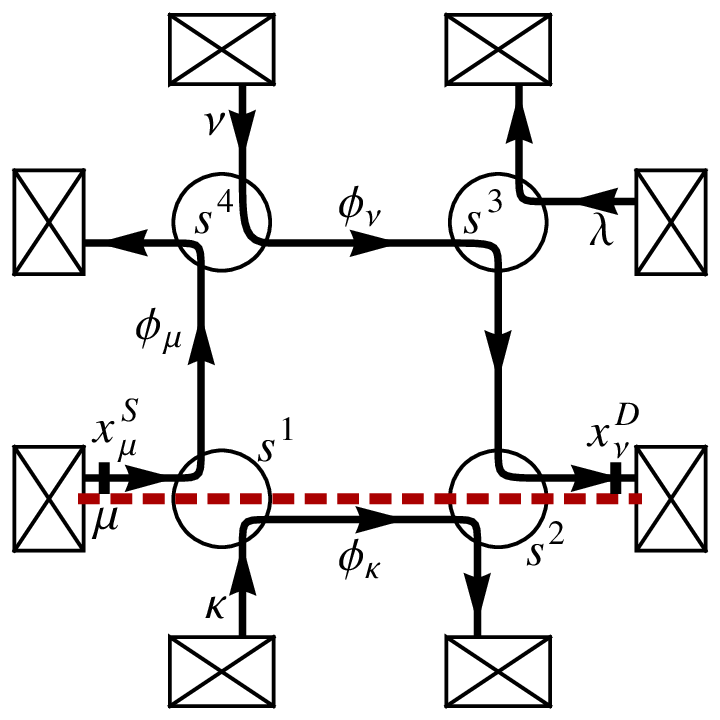
Let us now discuss how the S-matrix for the systems under consideration is constructed. The elements of Sν​μα​(t,t′)S^{\alpha}_{\nu\mu}(t,t^{\prime}) give the amplitude that a wave packet incident from source μ\mu at time t′t^{\prime} leaves the system at time tt through the drain ν\nu. They are sums Sν​μα​(t,t′)=∑μAμ(p)​α​(t,t′)S^{\alpha}_{\nu\mu}(t,t^{\prime})=\sum_{\mu}A^{(p)\alpha}_{\mu}(t,t^{\prime}) over all corresponding paths pp formed by elements of the network.

Refer to caption
Figure 2: Network built out of four channels μ,κ,ν,λ\mu,\kappa,\nu,\lambda and point scatterers 1,2,3,41,2,3,4. Counting fields measure outgoing currents. Along interior parts of channels classical phases ϕμ/κ/ν\phi_{\mu/\kappa/\nu}, e.g. due to magnetic field, are accumulated. An exemplary path pp is indicated by a dashed line.

Figure 2 shows an exemplary path pp through a network of channels and point scatterers. It consists of an alternating sequence of two types of processes:

Electron propagation in the potential φμα\varphi_{\mu}^{\alpha} between xix^{i} and xjx^{j},

leading to the accumulated phase

ϑμα(xj,xi;t)(t)≡−vμ−1∫xixjdxφμα(x,t−(xj−x)/vμ).\vartheta^{\alpha}_{\mu}(x^{j},x^{i};t)(t)\equiv-v^{-1}_{\mu}\int_{x^{i}}^{x^{j}}\!\mathrm{d}x\,\varphi^{\alpha}_{\mu}(x,t-(x^{j}-x)/v_{\mu}). (13)

In addition to the Hubbard-Stratonovich field φμα\varphi^{\alpha}_{\mu}, there may be other time-depending phases ϕμα\phi^{\alpha}_{\mu} (e.g., induced by a magnetic field) contributing to Eq. (13). Note that ϑμα​(x,xi)\vartheta^{\alpha}_{\mu}(x,x^{i}) satisfies the same differential equation (∂t+vμ∂x)ϑμα(x,xi;t)=−φμα(x,t)(\partial_{t}+v_{\mu}\partial_{x})\vartheta^{\alpha}_{\mu}(x,x^{i};t)=-\varphi^{\alpha}_{\mu}(x,t) as Θμα​(x,t)\Theta^{\alpha}_{\mu}(x,t), but has a simpler (“incomplete”) Keldysh structure which involves only the retarded/advanced components of the bare particle-hole propagator D0​μD_{0\mu}. We refer to ϑμα​(x,xi)\vartheta^{\alpha}_{\mu}(x,x^{i}) as a kinematic phase. To take a finite flight time of electron between xix^{i} and xjx^{j} into account, we introduce a “delay operator”

Δμ​(xj,xi,t′,t)=δ⁡(t′−t−(xj−xi)/vμ)\Delta_{\mu}(x^{j},x^{i};t^{\prime},t)=\delta(t^{\prime}-t-(x^{j}-x^{i})/v_{\mu}) (14)

Then the amplitude of this process reads

ℳμα​(xj,xi,t,t′)≡ei​ϑμα​(xj,xi,t)​Δμ​(xj,xi,t,t′).{\mathcal{M}}^{\alpha}_{\mu}(x^{j},x^{i};t,t^{\prime})\equiv e^{i\vartheta^{\alpha}_{\mu}(x^{j},x^{i};t)}\Delta_{\mu}(x^{j},x^{i};t,t^{\prime}). (15)

Indeed, consider the 1D version of the Schrödinger equation on a directed link xi→xjx^{i}\to x^{j},

i∂tψμ=(−ivμ∂x+ϕμα)ψμ.i\partial_{t}\psi_{\mu}=(-iv_{\mu}\partial_{x}+\phi_{\mu}^{\alpha})\psi_{\mu}. (16)

Using the definition of the kinematic phase (13), this equation can be solved independently one each branch of the Keldysh contour yielding the relation

ψμ​(xj,t)=ei​ϑμα​(xj,xi,t)​ψμ​(xi,t−(xj−xi)/vμ),\psi_{\mu}(x_{j},t)=e^{i\vartheta_{\mu}^{\alpha}(x^{j},x^{i};\,t)}\psi_{\mu}(x_{i},t-(x^{j}-x^{i})/v_{\mu}), (17)

which implies that the scattering matrix is given Eq. (15).

Scattering/tunneling at point scatterer jj:

The amplitude of instantaneous scattering from channel μ\mu to ν\nu is

sν​μj​(t′,t)=sν​μj​δ​(t′−t).\displaystyle s^{j}_{\nu\mu}(t^{\prime},t)=s^{j}_{\nu\mu}\delta(t^{\prime}-t).
Passing the charge detector at drain μ\mu, which is described by the counting field χμ\chi_{\mu}.

As a special variant of a., our formalism includes the theory of full counting statistics. A counting field residing in the drain lead μ\mu measures the current flowing in that drain. The corresponding amplitude is

𝒳μα​(t′,t)=e−i​α2​χμ​δ​(t′−t).\displaystyle\mathcal{X}^{\alpha}_{\mu}(t^{\prime},t)=e^{-i\frac{\alpha}{2}\chi_{\mu}}\delta(t^{\prime}-t).

Then the action (12) enables us to express the cumulant generating function of the network as a functional integral over φ\varphi,

𝒵⁡(χ→)=∫∏μ𝒟​φμ±​(x,t)​exp⁡{i​𝒜​(φ,χ→)},{\cal Z}(\vec{\chi})=\int\prod_{\mu}{\cal D}\varphi^{\pm}_{\mu}(x,t)\,\exp\left\{i{\cal A}(\,\varphi,\vec{\chi})\right\}, (18)

where vector χ→\vec{\chi} combines counting fields χμ\chi_{\mu} in all drains.

Finally, the amplitude Aν​μ(p)​αA^{(p)\alpha}_{\nu\mu} of a path pp is the path-ordered (real) time convolution (“latest to the left”) of the amplitudes of its constituent processes. As an example, the amplitude indicated by the dashed line in Fig. 2 reads

Aν​μ(p)​α​(t,t′)=[𝒳να​ℳνα​(xνD,xν2)​sν​κ2​ℳκα​(xκ2,xκ1)​sκ​μ1​ℳμα​(xμ1,xμS)]​(t,t′)=δ⁡(t−t′−τ)​e−i​α2​χν+i​ϕκ​sν​κ2​sκ​μ1​exp⁡{i​ϑνα​(xνD,xν2,t)+i​ϑκα​(xκ2,xκ1,t−τ3)+i​ϑμα​(xμ1,xμS,t−τ3−τ2)},A^{(p)\alpha}_{\nu\mu}(t,t^{\prime})=\left[\mathcal{X}^{\alpha}_{\nu}\ {\mathcal{M}}^{\alpha}_{\nu}(x^{D}_{\nu},x^{2}_{\nu})\ s^{2}_{\nu\kappa}\ {\mathcal{M}}^{\alpha}_{\kappa}(x^{2}_{\kappa},x^{1}_{\kappa})\ s^{1}_{\kappa\mu}\ {\mathcal{M}}^{\alpha}_{\mu}(x^{1}_{\mu},x^{S}_{\mu})\right](t,t^{\prime})\\ =\delta(t-t^{\prime}-\tau)\ e^{-i\frac{\alpha}{2}\chi_{\nu}+i\phi_{\kappa}}\ s^{2}_{\nu\kappa}s^{1}_{\kappa\mu}\ \exp\left\{i\vartheta^{\alpha}_{\nu}(x_{\nu}^{D},x^{2}_{\nu};t)+i\vartheta^{\alpha}_{\kappa}(x^{2}_{\kappa},x^{1}_{\kappa};t-\tau_{3})+i\vartheta^{\alpha}_{\mu}(x^{1}_{\mu},x_{\mu}^{S};t-\tau_{3}-\tau_{2})\right\}\,,

where τ1/2/3\tau_{1/2/3} denote the flight times of the subpaths xμS→xμ1x_{\mu}^{S}\to x^{1}_{\mu}, xκ1→xκ2x^{1}_{\kappa}\to x_{\kappa}^{2}, xν2→xνDx^{2}_{\nu}\to x_{\nu}^{D}, and τ=τ1+τ2+τ3\tau=\tau_{1}+\tau_{2}+\tau_{3} is the total flight time.

2.3 Weak Tunneling Expansion

Due to the complex temporal behavior of the scattering matrix analytical evaluation of the functional determinant (12) is not feasible in general. An approximate treatment is possible if a weak tunneling at the point scatterers is assumed (i.e. the scattering matrix sν​μjs^{j}_{\nu\mu} close to δν​μ\delta_{\nu\mu}), and the ultimate goal of this section is the expansion of the action in the tunneling strength. Since in the absence of tunneling the network is described by the Gaussian action (8), one can introduce the tunneling action 𝒜t​[φ]\mathcal{A}_{t}[\varphi], so that 𝒜⁡[φ]=𝒜0​[φ]+𝒜t​[φ]\mathcal{A}[\varphi]=\mathcal{A}_{0}[\varphi]+\mathcal{A}_{t}[\varphi], where the expansion of 𝒜t​[φ]\mathcal{A}_{t}[\varphi] starts from second-order terms with respect to the tunneling amplitudes at the point scatterers. In Appendix C we show that an exact representation of 𝒜t​[φ]\mathcal{A}_{t}[\varphi] is given in terms of a modified (“regularized”) functional determinant

𝒜t​[φ]=−i​ln⁡Det⁡[𝟙−f+S~+⁣†​S~−​f].\displaystyle\mathcal{A}_{t}[\varphi]=-i\ln\mathrm{Det}\,\left[\mathds{1}-f+{\tilde{S}}^{+\dagger}{\tilde{S}}^{-}f\right]. (19)

The new, “regularized” scattering matrix S~{\tilde{S}} here is constructed similarly to SS. Each of its elements S~ν​μα​(t,t′)=∑pA~ν​μ(p)​α​(t,t′){\tilde{S}}^{\alpha}_{\nu\mu}(t,t^{\prime})=\sum_{p}\tilde{A}^{(p)\alpha}_{\nu\mu}(t,t^{\prime}) is a sum over the same paths pp which contribute to Sν​μα​(t,t′)S^{\alpha}_{\nu\mu}(t,t^{\prime}) and connect the source μ\mu with the drain ν\nu. Full and regularized amplitudes, Aν​μ(p)A^{(p)}_{\nu\mu} and A~ν​μ(p)\tilde{A}^{(p)}_{\nu\mu} respectively, differ in the partial amplitudes assigned to the elementary processes a. and b. which constitute a path pp:

Propagation between xix^{i} and xjx^{j}.

Only the time delay is taken into account:

ℳ~μα​(xj,xi)=Δμ​(xj,xi),\displaystyle\tilde{\mathcal{M}}^{\alpha}_{\mu}(x^{j},x^{i})=\Delta_{\mu}(x^{j},x^{i}),

while phase accumulation is shifted to

Tunneling at point scatterers jj.

The off-diagonal tunneling amplitudes become “dressed” by tunneling phases Φν​μα​(xj,t)≡Θμα​(xμj,t)−Θνα​(xνj,t)\Phi^{\alpha}_{\nu\mu}(x^{j},t)\equiv\Theta^{\alpha}_{\mu}(x^{j}_{\mu},t)-\Theta^{\alpha}_{\nu}(x^{j}_{\nu},t):

s~ν​μj​α​(t,t′)=ei​Φν​μα​(xj,t)​sν​μj​δ​(t−t′).\displaystyle\tilde{s}^{j\alpha}_{\nu\mu}(t,t^{\prime})=e^{i\Phi^{\alpha}_{\nu\mu}(x^{j},t)}s^{j}_{\nu\mu}\delta(t-t^{\prime}).

The phases Θμ=−D0​μ​φμ\Theta_{\mu}=-D_{0\mu}\varphi_{\mu} are defined as in Sect. 2.1 and can be modified by additional time-independent phase contributions due to e.g. magnetic or counting fields as follows. If the additional phase accumulated by an electron which propagates along a channel μ\mu from a position xx to the drain lead μ\mu is denoted as ϕμ.outα​(x)\phi^{\alpha}_{\mu.\mathrm{out}}(x), then the phase Θμα\Theta^{\alpha}_{\mu} is modified according to

Θμα​(x,t)↦Θμα​(x,t)−ϕμ.outα​(x).\displaystyle\Theta^{\alpha}_{\mu}(x,t)\mapsto\Theta^{\alpha}_{\mu}(x,t)-\phi^{\alpha}_{\mu.\mathrm{out}}(x).

In our previous example, Fig. 2, the regularized scattering amplitudes read

s~κ​μ1​α​(t,t′)\displaystyle\tilde{s}_{\kappa\mu}^{1\alpha}(t,t^{\prime}) =ei​Φκ​μα​(x1,t)−i⁡(ϕμ−ϕκ)+i​α2​(χμ−χκ)​sκ​μ2​δ​(t−t′),\displaystyle=e^{i\Phi^{\alpha}_{\kappa\mu}(x^{1},t)-i\left(\phi_{\mu}-\phi_{\kappa}\right)+i\frac{\alpha}{2}\left(\chi_{\mu}-\chi_{\kappa}\right)}s^{2}_{\kappa\mu}\delta(t-t^{\prime}),
s~ν​κ1​α​(t,t′)\displaystyle\tilde{s}_{\nu\kappa}^{1\alpha}(t,t^{\prime}) =ei​Φν​κα​(x2,t)+i​α2​(χκ−χν)​sν​κ2​δ​(t−t′).\displaystyle=e^{i\Phi^{\alpha}_{\nu\kappa}(x^{2},t)+i\frac{\alpha}{2}\left(\chi_{\kappa}-\chi_{\nu}\right)}s^{2}_{\nu\kappa}\delta(t-t^{\prime}).

The regularized scattering matrix becomes trivial in the “clean” limit, S~=𝟙{\tilde{S}}=\mathds{1}, since all effects of interaction are now contained in the phases of the off-diagonal elements of the regularized scattering matrices s~ν​μj\tilde{s}_{\nu\mu}^{j} of connectors. Thus Eq. (19) can be expanded in (even) powers of the tunneling amplitudes:

𝒜t​[φ]=i​∑n=1∞1n​Tr​[(𝟙−S~+⁣†​S~−)​f]n.\displaystyle\mathcal{A}_{t}[\varphi]=i\sum_{n=1}^{\infty}\frac{1}{n}\mathrm{Tr}\,\left[\left(\mathds{1}-{\tilde{S}}^{+\dagger}{\tilde{S}}^{-}\right)f\right]^{n}.

We are now going to elaborate on the second-order terms in this series.

Second Order Expansion

We introduce a notation 𝒜≡S~+⁣†​S~−\mathcal{A}\equiv\tilde{S}^{+\dagger}\tilde{S}^{-}. Up to third order corrections in the tunneling amplitudes [that we denote as 𝒪⁡(tun3)\mathcal{O}(\mathrm{tun}^{3})] the tunneling action is

𝒜t​[φ]=\displaystyle\mathcal{A}_{t}[\varphi]= i​Tr​[(𝟙−𝒜)​f+12​(𝟙−𝒜)​f​(𝟙−𝒜)​f]+O⁡(tun3)\displaystyle i\mathrm{Tr}\,\left[(\mathds{1}-\mathcal{A})f+\frac{1}{2}(\mathds{1}-\mathcal{A})f(\mathds{1}-\mathcal{A})f\right]+O(\mathrm{tun}^{3})
=\displaystyle= i​Tr​[(𝟙−𝒜)μ​μ​fμ+12​∑μ≠ν𝒜μ​ν​fν​𝒜ν​μ​fμ]+O⁡(tun3).\displaystyle i\mathrm{Tr}\,\left[(\mathds{1}-\mathcal{A})_{\mu\mu}f_{\mu}+\frac{1}{2}\sum_{\mu\neq\nu}\mathcal{A}_{\mu\nu}f_{\nu}\mathcal{A}_{\nu\mu}f_{\mu}\right]+O(\mathrm{tun}^{3}). (20)

In the last expression, the trace is only taken with respect to time. To reduce the tunneling action to this form, we used (𝟙−𝒜)μ​μ=O⁡(tun2)(\mathds{1}-\mathcal{A})_{\mu\mu}=O(\mathrm{tun}^{2}) and 𝒜ν​μ=O⁡(tun)\mathcal{A}_{\nu\mu}=O(\mathrm{tun}).

It can be shown (see Appendix D for a detailed derivation) that 𝒜t\mathcal{A}_{t} acquires contributions from paths which start in a certain source reservoir, evolve forward and backward in time, undergoing in total exactly 2 tunneling events, and eventually returning to the original source. Such paths involve exactly 2 different channels, μ\mu and ν\nu. Thus we can classify all paths according to the pair (μ,ν)(\mu,\nu) of channels μ≠ν\mu\neq\nu and the pair (i,j)(i,j) of scatterers (possibly equal) at which the tunneling takes place: μ→ν\mu\to\nu at ii and ν→μ\nu\to\mu at jj. Of course, the class (i​j;μ​ν)(ij;\mu\nu) coincides with the class (j​i;ν​μ)(ji;\nu\mu). The second order expansion of the tunneling action then is a sum over these classes:

𝒜t[φ]=−i∑(i​j;μ​ν)∫dt1dt2(e−i​Φμ​ν−​(xi,t1)e−i​Φμ​ν+​(xi,t1))(Πi​j;μ​νT​(t12)−Πi​j;μ​ν<​(t12)−Πi​j;μ​ν>​(t12)Πi​j;μ​νT~​(t12))(ei​Φμ​ν−​(xj,t2)ei​Φμ​ν+​(xj,t2)),\displaystyle\mathcal{A}_{t}[\varphi]=-i\sum_{(ij;\mu\nu)}\int\!\!\mathrm{d}t_{1}\mathrm{d}t_{2}\,\begin{pmatrix}e^{-i\Phi^{-}_{\mu\nu}(x^{i},t_{1})}&e^{-i\Phi^{+}_{\mu\nu}(x^{i},t_{1})}\end{pmatrix}\begin{pmatrix}\Pi_{ij;\mu\nu}^{T}(t_{12})&-\Pi_{ij;\mu\nu}^{<}(t_{12})\\ -\Pi_{ij;\mu\nu}^{>}(t_{12})&\Pi_{ij;\mu\nu}^{\tilde{T}}(t_{12})\end{pmatrix}\begin{pmatrix}e^{i\Phi^{-}_{\mu\nu}(x^{j},t_{2})}\\ e^{i\Phi^{+}_{\mu\nu}(x^{j},t_{2})}\end{pmatrix}, (21)

t12≡t1−t2t_{12}\equiv t_{1}-t_{2}, where the tunneling polarization operators are given by

Πi​j;μ​ν≷​(t)\displaystyle\Pi^{\gtrless}_{ij;\mu\nu}(t) =−sν​μi​s¯ν​μj​ei​Δ​ϕμ​νi​j​e±i⁡(χμ−χν)​fμ≷​(t+τμ.inj−τμ.ini)​fν≶​(τν.ini−τν.inj−t),\displaystyle=-s^{i}_{\nu\mu}\bar{s}^{j}_{\nu\mu}\ e^{i\Delta\phi^{ij}_{\mu\nu}}e^{\pm i(\chi_{\mu}-\chi_{\nu})}f_{\mu}^{\gtrless}(t+\tau^{j}_{\mu.\mathrm{in}}-\tau^{i}_{\mu.\mathrm{in}})f_{\nu}^{\lessgtr}(\tau^{i}_{\nu.\mathrm{in}}-\tau^{j}_{\nu.\mathrm{in}}-t), (22)
Πi​j;μ​νT/T~​(t)\displaystyle\Pi^{T/{\tilde{T}}}_{ij;\mu\nu}(t) =[θ⁡(±t)​Πi​j;μ​ν>​(t)+θ⁡(∓t)​Πi​j;μ​ν<​(t)]χ≡0,\displaystyle=\left[\theta(\pm t)\Pi^{>}_{ij;\mu\nu}(t)+\theta(\mp t)\Pi^{<}_{ij;\mu\nu}(t)\right]_{\chi\equiv 0}\,, (23)

where τλ.ink\tau^{k}_{\lambda.\mathrm{in}} is the flight time from the source to the scatterer kk along a channel λ\lambda, τλ.ink=(xλk−xλS)/vλ\tau^{k}_{\lambda.\mathrm{in}}=(x^{k}_{\lambda}-x_{\lambda}^{S})/v_{\lambda}. We have also taken into account counting fields in the drain leads (which are not contained in Πi​j;μ​νT/T~\Pi^{T/{\tilde{T}}}_{ij;\mu\nu}) and classical phases,

Δ​ϕμ​νi​j≡ϕν.out​(xi)−ϕμ.out​(xi)−ϕν.out​(xj)+ϕμ.out​(xj).\displaystyle\Delta\phi^{ij}_{\mu\nu}\equiv\phi_{\nu.\mathrm{out}}(x^{i})-\phi_{\mu.\mathrm{out}}(x^{i})-\phi_{\nu.\mathrm{out}}(x^{j})+\phi_{\mu.\mathrm{out}}(x^{j}).

In the case i=ji=j we will also use the convention

Πi​i;μ​νT​(t)=Πi​i;μ​νT~​(t)=12​[Πi​i;μ​ν>​(t)+Πi​i;μ​ν<​(t)].\displaystyle\Pi^{T}_{ii;\mu\nu}(t)=\Pi^{\tilde{T}}_{ii;\mu\nu}(t)=\frac{1}{2}\left[\Pi^{>}_{ii;\mu\nu}(t)+\Pi^{<}_{ii;\mu\nu}(t)\right]. (24)

The comparison of this expression with the Eq. (23) shows that they differ from each other by the singular term proportional to sign⁡(t)​h​(t)​δ​(t)=π​δ2​(t){\rm sign}(t)h(t)\delta(t)=\pi\delta^{2}(t), where we put h⁡(t)=f0>​(t)−f0<​(t)h(t)=f^{>}_{0}(t)-f^{<}_{0}(t). It gives some constant (albeit infinite) contribution to the tunneling action (21) and therefore both representation for Πi​i;μ​νT/T~\Pi^{T/\tilde{T}}_{ii;\mu\nu} are equivalent.

2.4 Real-Time Instanton Method

On the level of the second order expansion, the action 𝒜t​[φ]\mathcal{A}_{t}[\varphi] is expressed in terms of the tunneling phases Φ\Phi, which are linear functionals of φ\varphi:

Φμ​ν​(ξ)=∑λ∫𝒞d​ξ′​𝒟μ​ν;λ​(ξ,ξ′)​φλ​(ξ′),𝒟μ​ν;λ≡D0​μ​δμ​λ−D0​ν​δν​λ.\Phi_{\mu\nu}(\xi)=\sum_{\lambda}\int_{\mathcal{C}}\mathrm{d}\xi^{\prime}\,{\mathcal{D}}_{\mu\nu;\lambda}(\xi,\xi^{\prime})\varphi_{\lambda}(\xi^{\prime}),\quad{\mathcal{D}}_{\mu\nu;\lambda}\equiv D_{0\mu}\delta_{\mu\lambda}-D_{0\nu}\delta_{\nu\lambda}. (25)

The action 𝒜t​[φ]\mathcal{A}_{t}[\varphi] is non-Gaussian in Φ\Phi and, in fact, is quite similar to the Ambegaokar-Eckern-Schön (AES) action [13]. The difference is that the kernel appearing in Eq. (21) is not only non-local in time (as in the case of AES) but in general is non-local in space as well. In view of the non-Gaussian character of the action an exact evaluation of physical quantities does not seem feasible in general. For this reason, we will use a saddle-point approximation that catches correctly the relevant interaction-induced physics, including both the renormalization and the dephasing phenomena.

To explain the idea of the method, let us consider some physical quantity 𝒪⁡[φ]=𝒪0​ei​𝒜J​[φ]\mathcal{O}[\varphi]=\mathcal{O}_{0}e^{i\mathcal{A}_{J}[\varphi]}, where 𝒜J[φ]=−∑μ∫𝒞dξJμ(ξ)φμ(ξ)\mathcal{A}_{J}[\varphi]=-\sum_{\mu}\int_{\mathcal{C}}\mathrm{d}\xi\,J_{\mu}(\xi)\varphi_{\mu}(\xi) is a linear functional of φ\varphi, and the prefactor 𝒪0\mathcal{O}_{0} is independent on φ\varphi. Important examples, which are treated in the next sections, include the electronic Green’s function and the current. The quantum average value of 𝒪{\mathcal{O}} is given by the functional integral

⟨𝒪⁡[φ]⟩=∫𝒟​φ​ei​𝒜0​[φ]+i​𝒜t​[φ]+i​𝒜J​[φ]​𝒪0,\displaystyle\left\langle\mathcal{O}[\varphi]\right\rangle=\int\mathcal{D}\varphi\,e^{i\mathcal{A}_{0}[\varphi]+i\mathcal{A}_{t}[\varphi]+i\mathcal{A}_{J}[\varphi]}\mathcal{O}_{0}, (26)

which we estimate in the semiclassical approximation [14]. In this case the path integral is contributed by the saddle-point trajectory φ∗⁣∗\varphi_{\ast\ast} of the full action 𝒜0​[φ]+𝒜t​[φ]+𝒜J​[φ]\mathcal{A}_{0}[\varphi]+\mathcal{A}_{t}[\varphi]+\mathcal{A}_{J}[\varphi] and quantum fluctuations around it. Here free and tunneling actions 𝒜0​[φ]\mathcal{A}_{0}[\varphi], 𝒜t​[φ]\mathcal{A}_{t}[\varphi] are given by Eqs. (8) and (21), respectively. In the limit of weak tunneling between chiral channels the saddle-point trajectory (“instanton” ) can be found approximately by requiring that it minimizes the Gaussian contributions to the action 𝒜0​[φ]+𝒜J​[φ]\mathcal{A}_{0}[\varphi]+\mathcal{A}_{J}[\varphi], which gives

φ∗μ​(ξ)=∑ν∫𝒞d​ξ′​Vμ​ν​(ξ,ξ′)​(ϱ0​ν​(ξ′)+Jν​(ξ′)).\displaystyle\varphi_{\ast\mu}(\xi)=\sum_{\nu}\int_{\mathcal{C}}\mathrm{d}\xi^{\prime}\,V_{\mu\nu}(\xi,\xi^{\prime})(\varrho_{0\nu}(\xi^{\prime})+J_{\nu}(\xi^{\prime})). (27)

As shown in Appendix E, under such an approximation Eq. (26) simplifies to

⟨𝒪⁡[φ]⟩=⟨ei​𝒜J​[φ]⟩0​ei​𝒜~t​[φ∗]​𝒪0,\displaystyle\left\langle\mathcal{O}[\varphi]\right\rangle=\left\langle e^{i\mathcal{A}_{J}[\varphi]}\right\rangle_{0}e^{i\tilde{\mathcal{A}}_{t}[\varphi_{\ast}]}\mathcal{O}_{0}\,, (28)

with

⟨ei​𝒜J​[φ]⟩0=exp⁡{i​⟨𝒜J​[φ]⟩0−12​[⟨(𝒜J​[φ]−⟨𝒜J​[φ]⟩0)2⟩0]},\displaystyle\left\langle e^{i\mathcal{A}_{J}[\varphi]}\right\rangle_{0}=\exp\left\{i\left\langle\mathcal{A}_{J}[\varphi]\right\rangle_{0}-\frac{1}{2}\left[\left\langle\left(\mathcal{A}_{J}[\varphi]-\left\langle\mathcal{A}_{J}[\varphi]\right\rangle_{0}\right)^{2}\right\rangle_{0}\right]\right\}, (29)
𝒜~t[φ∗]=−i∑{μ,ν},(i,j)∫dt1dt2(e−i​Φ∗μ​ν−​(xi,t1)e−i​Φ∗μ​ν+​(xi,t1))(Π~i​j;μ​νT​(t12)−Π~i​j;μ​ν<​(t12)−Π~i​j;μ​ν>​(t12)Π~i​j;μ​νT~​(t12))(ei​Φ∗μ​ν−​(xj,t2)ei​Φ∗μ​ν+​(xj,t2)),\displaystyle\tilde{\mathcal{A}}_{t}[\varphi_{\ast}]=-i\!\!\!\!\sum_{\{\mu,\nu\},(i,j)}\int\!\!\mathrm{d}t_{1}\mathrm{d}t_{2}\,\begin{pmatrix}e^{-i\Phi^{-}_{\ast\mu\nu}(x^{i},t_{1})}&e^{-i\Phi^{+}_{\ast\mu\nu}(x^{i},t_{1})}\end{pmatrix}\begin{pmatrix}\tilde{\Pi}_{ij;\mu\nu}^{T}(t_{12})&-\tilde{\Pi}_{ij;\mu\nu}^{<}(t_{12})\\ -\tilde{\Pi}_{ij;\mu\nu}^{>}(t_{12})&\tilde{\Pi}_{ij;\mu\nu}^{\tilde{T}}(t_{12})\end{pmatrix}\begin{pmatrix}e^{i\Phi^{-}_{\ast\mu\nu}(x^{j},t_{2})}\\ e^{i\Phi^{+}_{\ast\mu\nu}(x^{j},t_{2})}\end{pmatrix}, (30)

where t12≡t1−t2t_{12}\equiv t_{1}-t_{2} and ⟨…⟩0\langle\ldots\rangle_{0} denotes averaging with respect to 𝒜0​[φ]\mathcal{A}_{0}[\varphi]. We have introduced the instanton phases Φ∗μ​ν=𝒟μ​ν​φ∗\Phi_{\ast\mu\nu}={\mathcal{D}}_{\mu\nu}\varphi_{\ast} and the renormalized tunneling polarization operators

Π~i​j;μ​να​β​(t1−t2)=ei⁡(DΦ​μ​να​β​(xi,xj,t1−t2)−DΦ​μ​να​α​(0,0))​Πi​j;μ​να​β​(t1−t2),\displaystyle\tilde{\Pi}^{\alpha\beta}_{ij;\mu\nu}(t_{1}-t_{2})=e^{i\left(D^{\alpha\beta}_{\Phi\mu\nu}(x^{i},x^{j};t_{1}-t_{2})-D^{\alpha\alpha}_{\Phi\mu\nu}(0,0)\right)}\ \Pi^{\alpha\beta}_{ij;\mu\nu}(t_{1}-t_{2}), (31)

obtained by dressing of the bare tunneling polarization operators by phase-phase correlators

DΦ​μ​ν​(ξ1,ξ2)=∑κ​λ∫Cd​ξ′​d​ξ′′​𝒟μ​ν;κ​(ξ1,ξ′)​Vκ​λ​(ξ′,ξ′′)​𝒟μ​ν;λ​(ξ′′,ξ2).\displaystyle D_{\Phi\mu\nu}(\xi_{1},\xi_{2})=\sum_{\kappa\lambda}\int_{C}\mathrm{d}\xi^{\prime}\,\mathrm{d}\xi^{\prime\prime}\,{\mathcal{D}}_{\mu\nu;\kappa}(\xi_{1},\xi^{\prime})V_{\kappa\lambda}(\xi^{\prime},\xi^{\prime\prime}){\mathcal{D}}_{\mu\nu;\lambda}(\xi^{\prime\prime},\xi_{2}).

The meaning of Eq. (31) is that quantum fluctuations of tunneling phases renormalize the temporal dependence of tunneling polarization operators which lead to non-trivial (usually power-law) energy-dependence of tunneling coefficients.

In the next two sections we consider two important applications of our general approach.

3 Tunneling Density of States of Luttinger Liquid with Single Impurity

In this section we show how our formalism can be applied to the evaluation of the tunneling density of states (TDOS) of a nonequilibrium quantum wire containing a single impurity [9], as depicted in Fig. 3. On the experimental side, the interest to such a theoretical study is motivated by the recent development of the nonequilibrium tunneling spectroscopy of 1D nanostructures, including carbon nanotubes [15] and quantum Hall edges [16, 17, 18].

3.1 Model and Results

Refer to caption
Figure 3: Tunneling experiment with a voltage-biased quantum wire.

The wire is modeled as a network of two channels: right- (left-) moving electrons, denoted with indices μ=+(−)\mu=+(-). Backscattering, i.e. tunneling between the two channels, occurs at the impurity (at x=0x=0) which is considered as a point scatterer with scattering matrix ss. Non-equilibrium conditions are established by biasing the right reservoir with respect to the left one: e​V+=e​V>0eV_{+}=eV>0, e​V−=0eV_{-}=0.

The interplay of interaction, nonequilibrium, and impurity scattering can be studied by placing a conducting tip held at a voltage VtipV_{\rm tip} near a position x¯\bar{x} of the wire (we can assume without loss of generality that x¯>0\bar{x}>0) and measuring the current ItunI_{\mathrm{tun}} between between tip and wire. Let us assume that the tip can be described in terms of fermionic quasiparticles with density of states νtip​(ϵ)\nu_{\rm tip}(\epsilon) and distribution function ftip​(ϵ)f_{\rm tip}(\epsilon), as is the case, e.g., in the absence of interaction within the tip. If the coupling |t|2\lvert t\rvert^{2} between the tip and the wire is weak, a simple perturbative expansion yields the tunneling current

Itun∝|t|2∑μ=±∫dϵ[Γμ>(ϵ)ftip(ϵ)−Γμ<(ϵ)(1−ftip(ϵ))]νtip(ϵ).\displaystyle I_{\mathrm{tun}}\propto\lvert t\rvert^{2}\sum_{\mu=\pm}\int\!\!\mathrm{d}\epsilon\left[\Gamma_{\mu}^{>}(\epsilon)f_{\rm tip}(\epsilon)-\Gamma^{<}_{\mu}(\epsilon)(1-f_{\rm tip}(\epsilon))\right]\nu_{\rm tip}(\epsilon).

The “rates” for tunneling into/out of the μ\mu-channel of the wire are defined as

Γμ≷​(ϵ)=±i2​π​Gμ≷​(x¯,x¯,ϵ).\displaystyle\Gamma^{\gtrless}_{\mu}(\epsilon)=\pm\frac{i}{2\pi}G_{\mu}^{\gtrless}(\bar{x},\bar{x},\epsilon). (32)

Measurement of a differential tunneling conductance in the limit of a small temperature gives the access to the tunneling density of states, since

∂Itun∂V|Vtip=ϵ∝Γμ>​(ϵ)+Γμ<​(ϵ)=νμ​(ϵ)≡−1π​Im​Gμr​(x¯,x¯,ϵ).\frac{\partial I_{\mathrm{tun}}}{\partial V}\bigg|_{V_{\rm tip}=\epsilon}\propto\,\Gamma^{>}_{\mu}(\epsilon)+\Gamma^{<}_{\mu}(\epsilon)=\nu_{\mu}(\epsilon)\equiv-\frac{1}{\pi}{\rm Im}\,G_{\mu}^{r}(\bar{x},\bar{x},\epsilon)\,. (33)

In the absence of interaction, the rates would simplify to Γμ≷​(ϵ)=fμ≷​(ϵ)​νμ​(ϵ)\Gamma_{\mu}^{\gtrless}(\epsilon)=f^{\gtrless}_{\mu}(\epsilon)\nu_{\mu}(\epsilon) with the distribution functions fμ<​(ϵ)=fμ​(ϵ)f_{\mu}^{<}(\epsilon)=f_{\mu}(\epsilon), fμ>​(ϵ)≡1−fμ​(ϵ)f^{>}_{\mu}(\epsilon)\equiv 1-f_{\mu}(\epsilon) and the density of states νμ​(ϵ)\nu_{\mu}(\epsilon) in the channel μ\mu. Evaluation of tunneling rates and of the TDOS of the interacting problem is the goal of this section.

We consider a spinless LL model with a point-like repulsive interaction, Uμ​ν​(x,x′)=V0​δ​(x−x′)U_{\mu\nu}(x,x^{\prime})=V_{0}\delta(x-x^{\prime}), that does not discriminate between different channels. The interaction strength in the LL model is conventionally characterized by the constant K=(1+V0/πvF)−1/2K=(1+V_{0}/\pi{v_{F}})^{-1/2}. The free electron spectrum is linearized around the Fermi points, which requires the introduction of a high-energy cutoff Λ∼EF\Lambda\sim E_{F} (which is of the order of the bandwidth). In the absence of backscattering, the tunneling rates exhibit the well-known zero bias anomaly, i.e. a power-law suppression near the Fermi edges,

Γμ≷​(ϵ)=ν0π​Γ​(1+2​γ)−1×θ⁡(±(ϵ−e​Vμ))​|ϵ−e​VμΛ|2​γ\Gamma_{\mu}^{\gtrless}(\epsilon)=\frac{\nu_{0}}{\pi}\Gamma(1+2\gamma)^{-1}\times\theta(\pm(\epsilon-eV_{\mu}))\left\lvert\frac{\epsilon-eV_{\mu}}{\Lambda}\right\rvert^{2\gamma}\quad (34)

where ν0=(2​π​vF)−1\nu_{0}=(2\pi{v_{F}})^{-1} is the non-interacting density of states, and the exponent γ\gamma is given by

γ=(1−K)24​K.\gamma=\frac{(1-K)^{2}}{4K}\,. (35)

As is shown in the remainder of this section the tunneling rates change considerably upon including the impurity. For e​V>0eV>0 the rates are given by

Γμ≷​(ϵ)=±ν0π​(e​VΛ)2​γ​Γ​(−2​γ)​Im​[(∓zμ)2​γ+𝒞μ​R∗​(e​V)​(±1)2​γ​Ψ​(−2​γ,1−2​γ+2​δμ,−1−zμ)],\Gamma^{\gtrless}_{\mu}(\epsilon)=\pm\frac{\nu_{0}}{\pi}\left(\frac{eV}{\Lambda}\right)^{2\gamma}\Gamma(-2\gamma)\ \mathrm{Im}\,\left[(\mp z_{\mu})^{2\gamma}+\mathcal{C}_{\mu}R_{\ast}(eV)(\pm 1)^{2\gamma}\Psi(-2\gamma,1-2\gamma+2\,\delta_{\mu},-1-z_{\mu})\right]\,, (36)

where we have introduced the following notations:

𝒞±=Γ⁡(2​K)Γ​(1/2±K/2)2,δ+=(1−K)/2,δ−=1/2−K,zμ=(ϵ−e​Vμ+i2​τφ−1)/e​V.\mathcal{C}_{\pm}=\frac{\Gamma(2K)}{\Gamma\left(1/2\pm K/2\right)^{2}},\quad\delta_{+}=(1-K)/2,\quad\delta_{-}=1/2-K,\quad z_{\mu}=(\epsilon-eV_{\mu}+\frac{i}{2}\tau_{\varphi}^{-1})/eV. (37)

We have also introduced the renormalized reflection coefficient

R∗​(e​V)=|r0|2Γ⁡(2​K)​|Λe​V|2​(1−K)\displaystyle R_{\ast}(eV)=\frac{\lvert r_{0}\rvert^{2}}{\Gamma(2K)}\left\lvert\frac{\Lambda}{eV}\right\rvert^{2(1-K)} (38)

and the nonequilibrium dephasing rate

τφ−1≡R∗​(e​V)​2​sin2⁡π​δ+π​|e​V|.\displaystyle\tau_{\varphi}^{-1}\equiv R_{\ast}(eV)\frac{2\sin^{2}\pi\delta_{+}}{\pi}\lvert eV\rvert. (39)
Refer to caption
Refer to caption
Refer to caption
Refer to caption
Figure 4: Tunneling rates for right- and left-movers with different interaction strengths: K=0.3K=0.3 (1), K=0.5K=0.5 (2), and K=0.75K=0.75 (3). Fermi edge for right-(left-) movers is at e​V+=e​VeV_{+}=eV (e​V−=0eV_{-}=0).

The energy dependence of rates Γ±≷​(ϵ)\Gamma^{\gtrless}_{\pm}(\epsilon) is shown in Fig. 4. The main feature of these plots is that the tunneling rates have split power-law singularities which are characterized by different exponents and are smeared by the nonequilibrium dephasing rate 1/τφ1/\tau_{\varphi}. The main edges are located at the corresponding chemical potentials, i.e., at ϵ=e​V±\epsilon=eV_{\pm} in the case of right-/left-moving states, respectively, and are characterized by the exponent equal (in the considered weak-back-scattering regime) to its equilibrium value γ\gamma. The formation of the second (side) edge due to scattering off the impurity occurs at ϵ=e⁡(V±−V)\epsilon=e(V_{\pm}-V). If the interaction is repulsive (K<1K<1) then the corresponding exponent 2​(γ−δ−)2(\gamma-\delta_{-}) for left-moving electrons is always positive, hence the correction at the side edge ϵ=0\epsilon=0 is smooth. For right-movers in the case of not too strong interaction, K>1/3K>1/3, the nonequilibrium exponent 2​(γ−δ+)2(\gamma-\delta_{+}) is negative, yielding a resonance in tunneling at the side edge ϵ=0\epsilon=0.

The presence of side edges in the tunneling rates can be understood in the following way. Inelastic electron backscattering at the impurity at point x=0x=0 induces the emission of real nonequilibrium plasmons with typical frequencies ℏ​ω≤e​V\hbar\omega\leq eV, which in the non-dissipative LL can propagate to the distant point of tunneling x¯\bar{x}. As the result, inelastic tunneling with absorption or stimulated emission of these real plasmons become possible. For example, an electron tunneling into the right/left moving state of the LL with the energy ϵ<e​V±\epsilon<eV_{\pm} can accommodate itself above the corresponding Fermi energy (e​V±eV_{\pm}) by picking up the quantum ℏ​ω>|ϵ|\hbar\omega>|\epsilon| from the nonequilibrium plasmon bath. Since the energy of out-of-equilibrium plasmons is limited by the applied voltage, one has a threshold: ϵ>e⁡(V±−V)\epsilon>e(V_{\pm}-V), which is developed into the power-law singularity typical for the LL. The singularity at the side edge of the tunneling rate-out describes the inverse processes: the inelastic tunneling from the LL accompanied by the stimulated emission of nonequilibrium plasmons with typical energy ℏ​ω≃e​V\hbar\omega\simeq eV. Such side edge is pronounced in the case of right-moving states only, Γ+<​(ϵ)\Gamma^{<}_{+}(\epsilon), and is not seen for the left-moving states, Γ−<​(ϵ)\Gamma^{<}_{-}(\epsilon), since the associated exponent 2​(γ−δ−)2(\gamma-\delta_{-}) is always positive in the latter case.

Having announced the main results, we now turn to details of their derivation.

3.2 Calculations

3.2.1 Action

Since interaction does not discriminate between channels μ,ν=±\mu,\nu=\pm, it can be decoupled by a Hubbard-Stratonovich transformation introducing a single field φ\varphi, i.e. φ+=φ−=φ\varphi_{+}=\varphi_{-}=\varphi. For weak backscattering, i.e. weak tunneling between right- and left-moving states at the impurity, the action 𝒜⁡[φ]=𝒜0​[φ]+𝒜t​[φ]\mathcal{A}[\varphi]=\mathcal{A}_{0}[\varphi]+\mathcal{A}_{t}[\varphi] is obtained according to Sect. 2.3. The free action (8) is

𝒜0​[φ]=12​∫𝒞d​ξ​d​ξ′​φ​(ξ)​V−1​(ξ−ξ′)​φ​(ξ′)−∑μ∫𝒞d​ξ​φ​(ξ)​(ϱ0++ϱ0−)\displaystyle\mathcal{A}_{0}[\varphi]=\frac{1}{2}\int_{\mathcal{C}}\mathrm{d}\xi\,\mathrm{d}\xi^{\prime}\,\varphi(\xi)V^{-1}(\xi-\xi^{\prime})\varphi(\xi^{\prime})-\sum_{\mu}\int_{\mathcal{C}}\mathrm{d}\xi\,\varphi(\xi)\left(\varrho_{0+}+\varrho_{0-}\right)

with ξ=(x,t)\xi=(x,t), non-local effective interaction V−1​(ξ−ξ′)=V0−1​δ​(ξ−ξ′)−Π⁡(ξ−ξ′)V^{-1}(\xi-\xi^{\prime})=V_{0}^{-1}\delta(\xi-\xi^{\prime})-\Pi(\xi-\xi^{\prime}) and the total polarization operator Π⁡(ξ)=Π+​(ξ)+Π−​(ξ)\Pi(\xi)=\Pi_{+}(\xi)+\Pi_{-}(\xi). Using (10) one obtains for the retarded/advanced components of effective interaction

Vr/a​(ω,p)=V0​ω2−vF2​p2ω±2−u2​p2\displaystyle V^{r/a}(\omega,p)=V_{0}\frac{\omega^{2}-{v_{F}}^{2}p^{2}}{\omega_{\pm}^{2}-u^{2}p^{2}} (40)

with a plasmon velocity u=vF/Ku={v_{F}}/K. (For a repulsive interaction K<1K<1, so that u>vFu>{v_{F}}.)

Since we are dealing with a single scatterer, the tunneling (or, equivalently, backscattering) action 𝒜t\mathcal{A}_{t}, as given by (21), consists of one term [corresponding to class (11;+−)(11;+-)]:

𝒜t[φ]=−i∫dt1dt2(e−i​Φ−​(t1)e−i​Φ+​(t1))(Π+⁣−T−Π+⁣−<−Π+⁣−>Π+⁣−T~)t1−t2(ei​Φ−​(t2)ei​Φ+​(t2)),\displaystyle\mathcal{A}_{t}[\varphi]=-i\int\!\!\mathrm{d}t_{1}\mathrm{d}t_{2}\,\begin{pmatrix}e^{-i\Phi^{-}(t_{1})}&e^{-i\Phi^{+}(t_{1})}\end{pmatrix}\begin{pmatrix}\Pi_{+-}^{T}&-\Pi_{+-}^{<}\\ -\Pi_{+-}^{>}&\Pi_{+-}^{\tilde{T}}\end{pmatrix}_{t_{1}-t_{2}}\begin{pmatrix}e^{i\Phi^{-}(t_{2})}\\ e^{i\Phi^{+}(t_{2})}\end{pmatrix}, (41)

where Φ∓​(t)=Θ−∓​(0,t)−Θ+∓​(0,t)\Phi^{\mp}(t)=\Theta^{\mp}_{-}(0,t)-\Theta^{\mp}_{+}(0,t) is the tunneling phase evaluated at the impurity, x=0x=0. The phases are related to the Hubbard-Stratonovich field φ\varphi according to (2). The tunneling polarization operator Π+⁣−=Π11;+−\Pi_{+-}=\Pi_{11;+-} is given by Eqs. (22), (23). The components of the polarization operator read

Π+⁣−≷​(t)\displaystyle\Pi^{\gtrless}_{+-}(t) =−|r0|2​f+≷​(t)​f−≶​(−t)=−|r0|2​e−i​e​V​t​[f0≷​(t)]2,\displaystyle=-\lvert r_{0}\rvert^{2}f_{+}^{\gtrless}(t)f^{\lessgtr}_{-}(-t)=-\lvert r_{0}\rvert^{2}e^{-ieVt}\left[f^{\gtrless}_{0}(t)\right]^{2}, (42)
Π+⁣−T/T~​(t)\displaystyle\Pi^{T/{\tilde{T}}}_{+-}(t) =12​[Π+⁣−>​(t)+Π+⁣−<​(t)].\displaystyle=\frac{1}{2}\left[\Pi^{>}_{+-}(t)+\Pi^{<}_{+-}(t)\right]. (43)

where |r0|2=|s+⁣−1|2=|s−⁣+1|2\lvert r_{0}\rvert^{2}=\lvert s^{1}_{+-}\rvert^{2}=\lvert s^{1}_{-+}\rvert^{2} is the bare reflection coefficient. We note that in Ref. [9] different notations were used: 𝒜b\mathcal{A}_{b} instead of 𝒜0​[φ]\mathcal{A}_{0}[\varphi], 𝒜imp\mathcal{A}_{\rm imp} instead of 𝒜t​[φ]\mathcal{A}_{t}[\varphi], and ϑ\vartheta instead of Θ\Theta. We also note that Eq. (43) is slightly different from Eq. (23); however, this difference leads only to an additional constant contribution to the action that is physically irrelevant.

3.2.2 Green’s Functions in Instanton Approximation

In order to find the tunneling rates, we represent the electron Green’s function at the point of tunneling x¯>0\bar{x}>0 as a path integral over the field φ\varphi,

Gμ≷​(x¯,x¯,t¯)=∫𝒟​φ​ei​𝒜​[φ]​ei​Θμ±​(x¯​t¯)​Gμ≷​(x¯,x¯,t¯,[φ])​e−i​Θμ∓​(x¯,0).\displaystyle G^{\gtrless}_{\mu}(\bar{x},\bar{x};\bar{t})=\int\mathcal{D}\varphi\,e^{i\mathcal{A}[\varphi]}e^{i\Theta^{\pm}_{\mu}(\bar{x}\bar{t})}G^{\gtrless}_{\mu}(\bar{x},\bar{x};\bar{t};[\varphi])e^{-i\Theta^{\mp}_{\mu}(\bar{x},0)}.

Here, Gμ​(x¯,x¯,t¯,[φ])G_{\mu}(\bar{x},\bar{x};\bar{t},[\varphi]) denotes the Green’s function for a given configuration of φ\varphi. It satisfies the Dyson equation with the spatially local self-energy

Σμ​[φ]​(x,x′,t,t′)=i​δ​(x)​δ​(x′)​(|r0|2​vF/2)​ei​μ​Φ​(t)​g−μ​(t−t′)​e−i​μ​Φ​(t′),\displaystyle\Sigma_{\mu}[\varphi](x,x^{\prime};t,t^{\prime})=i\delta(x)\delta(x^{\prime})(\lvert r_{0}\rvert^{2}{v_{F}}/2)e^{i\mu\Phi(t)}g_{-\mu}(t-t^{\prime})e^{-i\mu\Phi(t^{\prime})}\,,

where gμg_{\mu} are the quasiclassical Green’s functions of the source reservoirs. Solving the Dyson equation to the first order in |r0|2\lvert r_{0}\rvert^{2}, we get

Gμα​β​(x¯,x¯,t¯)=𝒢0​μα​β+𝒢1​μα​β,G_{\mu}^{\alpha\beta}(\bar{x},\bar{x};\bar{t})=\mathcal{G}^{\alpha\beta}_{0\mu}+\mathcal{G}^{\alpha\beta}_{1\mu}\,, (44)

where

𝒢0​μα​β=\displaystyle\mathcal{G}^{\alpha\beta}_{0\mu}= ⟨ei​Θμα​(x¯,t¯)​G0​μα​β​(x¯,x¯,t¯)​e−i​Θμβ​(x¯,0)⟩,\displaystyle\left\langle e^{i\Theta^{\alpha}_{\mu}(\bar{x},\bar{t})}G^{\alpha\beta}_{0\mu}(\bar{x},\bar{x};\bar{t})e^{-i\Theta^{\beta}_{\mu}(\bar{x},0)}\right\rangle,
𝒢1​μα​β=\displaystyle\mathcal{G}^{\alpha\beta}_{1\mu}= i|r0|2​vF2∑γδ=∓γδ∫dt1dt2\displaystyle i\frac{\lvert r_{0}\rvert^{2}{v_{F}}}{2}\sum_{\gamma\delta=\mp}\gamma\delta\int\!\!\mathrm{d}t_{1}\,\mathrm{d}t_{2}\, (45)
⟨ei​Θμα​(x¯,t¯)​G0​μα​γ​(x¯,0,t¯−t1)​ei​μ​Φγ​(t1)​g−μγ​δ​(t1−t2)​e−i​μ​Φδ​(t2)​G0​μδ​β​(0,x¯,t2−t¯)​e−i​Θμβ​(x¯,0)⟩.\displaystyle\left\langle e^{i\Theta^{\alpha}_{\mu}(\bar{x},\bar{t})}G_{0\mu}^{\alpha\gamma}(\bar{x},0;\bar{t}-t_{1})e^{i\mu\Phi^{\gamma}(t_{1})}g^{\gamma\delta}_{-\mu}(t_{1}-t_{2})e^{-i\mu\Phi^{\delta}(t_{2})}G_{0\mu}^{\delta\beta}(0,\bar{x};t_{2}-\bar{t})e^{-i\Theta^{\beta}_{\mu}(\bar{x},0)}\right\rangle. (46)

Here G0​μα​βG_{0\mu}^{\alpha\beta} are the Green’s functions of free electrons; in particular,

G0​μ≷(x,t)=±f≷(t−μx/vF)/ivF.G^{\gtrless}_{0\mu}(x,t)=\pm f^{\gtrless}(t-\mu x/{v_{F}})/i{v_{F}}. (47)

All averages ⟨…⟩\langle\ldots\rangle in Eq. (46) are taken with respect to the action 𝒜0​[φ]+𝒜t​[φ]\mathcal{A}_{0}[\varphi]+\mathcal{A}_{t}[\varphi]. They are of the form (26) and can be evaluated with the real-time instanton method described in Sect. 2.4. In this approximation the first term in Eq. (44) reads

𝒢0​μα​β≈ei​𝒜~t​[φ∗]×⟨ei​Θμ±​(x¯,t¯)​G0​μ≷​(x¯,x¯,t¯)​e−i​Θμ∓​(x¯,0)⟩0.\mathcal{G}_{0\mu}^{\alpha\beta}\approx e^{i\tilde{\mathcal{A}}_{t}[\varphi_{\ast}]}\times\left\langle e^{i\Theta^{\pm}_{\mu}(\bar{x},\bar{t})}G^{\gtrless}_{0\mu}(\bar{x},\bar{x};\bar{t})e^{-i\Theta^{\mp}_{\mu}(\bar{x},0)}\right\rangle_{0}. (48)

The second factor here is the full Green’s function of a clean LL,

G~0​μ≷​(x¯,x¯,t¯)=e−12​⟨[Θμ±​(x¯,t¯)−Θμ∓​(x¯,0)]2⟩0​G0​μ≷​(x¯,x¯,t¯)=±a2​γ2​π​i​vF​e−i​μμ​t¯​1(a±i​t¯)2​γ+1.\displaystyle\tilde{G}_{0\mu}^{\gtrless}(\bar{x},\bar{x};\bar{t})=e^{-\frac{1}{2}\left\langle\left[\Theta_{\mu}^{\pm}(\bar{x},\bar{t})-\Theta^{\mp}_{\mu}(\bar{x},0)\right]^{2}\right\rangle_{0}}\ G_{0\mu}^{\gtrless}(\bar{x},\bar{x};\bar{t})=\pm\frac{a^{2\gamma}}{2\pi i{v_{F}}}e^{-i\mu_{\mu}\bar{t}}\frac{1}{(a\pm i\bar{t})^{2\gamma+1}}. (49)

The first factor in Eq. (48) gives dephasing corrections due to the interplay of tunneling and interaction. The instanton action 𝒜~t​[φ∗]\tilde{\mathcal{A}}_{t}[\varphi_{\ast}] is defined in (30) and obtained by substituting the dressed polarization operators into (41). The instanton phase φ∗\varphi_{\ast} is generated by the source i​𝒜J​[φ]=i​Θμα​(x¯,t¯)−i​Θμβ​(x¯,0)i\mathcal{A}_{J}[\varphi]=i\Theta_{\mu}^{\alpha}(\bar{x},\bar{t})-i\Theta^{\beta}_{\mu}(\bar{x},0),

Φ∗∓​(t)=⟨Φ∓​(t)⟩0−DΦ​Θ​μ∓α​(t−t¯,−x¯)+DΦ​Θ​μ∓β​(t,−x¯)​with​DΦ​Θ​μγ​δ​(t,x)=DΘ,−μγ​δ​(t,x)−DΘ,+μγ​δ​(t,x),\displaystyle\Phi^{\mp}_{\ast}(t)=\left\langle\Phi^{\mp}(t)\right\rangle_{0}-D_{\Phi\Theta\mu}^{\mp\alpha}(t-\bar{t},-\bar{x})+D^{\mp\beta}_{\Phi\Theta\mu}(t,-\bar{x})\ \text{with}\ D^{\gamma\delta}_{\Phi\Theta\mu}(t,x)=D^{\gamma\delta}_{\Theta,-\mu}(t,x)-D^{\gamma\delta}_{\Theta,+\mu}(t,x), (50)

and depends on Keldysh indices α,β\alpha,\beta, the direction μ\mu of the tunneling electron, as well as the time and the position of tunneling t¯\bar{t}, x¯\bar{x}. Since the average value ⟨Φ∓​(t)⟩0\left\langle\Phi^{\mp}(t)\right\rangle_{0} does not depend on the Keldysh index ∓\mp and the time tt it will drop out when the instanton phase is substituted into (41). Therefore it will be omitted in what follows.

3.2.3 Phase-phase Correlation Functions

To lay the groundwork for all further calculations we compute the correlation functions of the phases Θμ\Theta_{\mu} and Φ=Θ−−Θ+\Phi=\Theta_{-}-\Theta_{+}. With the bare particle-hole propagator (4), the effective interaction (40), and the relation (11), the retarded/advanced components of the correlators DΘ,μ​νD_{\Theta,\mu\nu} can be easily evaluated in the (q,ω)(q,\omega) representation:

DΘ,μ​μr/a​(ω,q)\displaystyle D^{r/a}_{\Theta,\mu\mu}(\omega,q) =−2​πω​ω+μ​vF​qω​μ​[1+K4​K​1q−μ​ω±/u−1−K4​K​1q+μ​ω±/u−12​1q−μ​ω±/vF],\displaystyle=-\frac{2\pi}{\omega}\frac{\omega+\mu{v_{F}}q}{\omega}\mu\left[\frac{1+K}{4K}\frac{1}{q-\mu\omega_{\pm}/u}-\frac{1-K}{4K}\frac{1}{q+\mu\omega_{\pm}/u}-\frac{1}{2}\frac{1}{q-\mu\omega_{\pm}/{v_{F}}}\right], (51)
DΘ,−μ​μr/a​(ω,q)\displaystyle D^{r/a}_{\Theta,-\mu\mu}(\omega,q) =−2​πω​1−K24​K​[1q−ω±/u+1q+ω±/u].\displaystyle=-\frac{2\pi}{\omega}\frac{1-K^{2}}{4K}\left[\frac{1}{q-\omega_{\pm}/u}+\frac{1}{q+\omega_{\pm}/u}\right]. (52)

Transforming the above relations into the mixed space-frequency representation, we obtain

DΘ,μ​νr/a(ω,x)=∓2​π​iω{θ(±μx)[cμ​ν+ei​μ​ω​x/u−δμ​νei​μ​ω/vF]+θ(∓μx)cμ​ν−e−iμωx/u}D^{r/a}_{\Theta,\mu\nu}(\omega,x)=\mp\frac{2\pi i}{\omega}\left\{\theta(\pm\mu x)\left[c^{+}_{\mu\nu}\ e^{i\mu\omega x/u}-\delta_{\mu\nu}\ e^{i\mu\omega/{v_{F}}}\right]+\theta(\mp\mu x)\ c^{-}_{\mu\nu}\ e^{-i\mu\omega x/u}\right\} (53)

with

cμ​μ±=(1±K)2/(4​K),cμ,−μ±=(1−K2)/(4​K).c^{\pm}_{\mu\mu}=(1\pm K)^{2}/(4K),\quad c^{\pm}_{\mu,-\mu}=(1-K^{2})/(4K). (54)

The Keldysh component of the phase correlator is given at zero temperature by

DΘ,μ​νk​(ω,x)=B⁡(ω)​(DΘ,μ​νr​(ω,x)−DΘ,μ​νa​(ω,x))=sign​ω​(DΘ,μ​νr​(ω,x)−DΘ,μ​νa​(ω,x)).D^{k}_{\Theta,\mu\nu}(\omega,x)=B(\omega)\left(D^{r}_{\Theta,\mu\nu}(\omega,x)-D^{a}_{\Theta,\mu\nu}(\omega,x)\right)=\mathrm{sign}\,\omega\ \left(D^{r}_{\Theta,\mu\nu}(\omega,x)-D^{a}_{\Theta,\mu\nu}(\omega,x)\right)\,. (55)

Performing the Keldysh rotation, we then arrive at

DΘ,μ​ν≷​(ω,x)=12​(DΘ,μ​νk​(ω,x)±(DΘ,μ​νr​(ω,x)−DΘ,μ​νa​(ω,x)))=±θ⁡(±ω)​(DΘ,μ​νr​(ω,x)−DΘ,μ​νa​(ω,x)),DΘ,μ​νT/T~​(ω,x)=12​(DΘ,μ​νk​(ω,x)±(DΘ,μ​νr​(ω,x)+DΘ,μ​νa​(ω,x)))=±θ⁡(±ω)​DΘ,μ​νr​(ω,x)±θ⁡(∓ω)​DΘ,μ​νa​(ω,x).\displaystyle\begin{split}D^{\gtrless}_{\Theta,\mu\nu}(\omega,x)&=\frac{1}{2}\left(D^{k}_{\Theta,\mu\nu}(\omega,x)\pm\left(D^{r}_{\Theta,\mu\nu}(\omega,x)-D^{a}_{\Theta,\mu\nu}(\omega,x)\right)\right)=\pm\theta(\pm\omega)\left(D^{r}_{\Theta,\mu\nu}(\omega,x)-D^{a}_{\Theta,\mu\nu}(\omega,x)\right),\\ D^{T/{\tilde{T}}}_{\Theta,\mu\nu}(\omega,x)&=\frac{1}{2}\left(D^{k}_{\Theta,\mu\nu}(\omega,x)\pm\left(D^{r}_{\Theta,\mu\nu}(\omega,x)+D^{a}_{\Theta,\mu\nu}(\omega,x)\right)\right)=\pm\theta(\pm\omega)D^{r}_{\Theta,\mu\nu}(\omega,x)\pm\theta(\mp\omega)D^{a}_{\Theta,\mu\nu}(\omega,x).\end{split} (56)

In the real-time representation (x,t)(x,t) these phase-phase correlation functions can be decomposed into the plasmon (moving with velocity uu) and particle-hole (having velocity vFv_{F}) contributions

i​DΘ,μ​να​β​(t,x)=cμ​ν+​ℒμ​uα​β​(t,x)−cμ​ν−​ℒ−μ​uα​β​(t,x)−δμ​ν​ℒμ​vFα​β​(t,x),\displaystyle iD_{\Theta,\mu\nu}^{\alpha\beta}(t,x)=c^{+}_{\mu\nu}\ \mathcal{L}^{\alpha\beta}_{\mu u}(t,x)-c^{-}_{\mu\nu}\ \mathcal{L}^{\alpha\beta}_{-\mu u}(t,x)-\delta_{\mu\nu}\ \mathcal{L}^{\alpha\beta}_{\mu{v_{F}}}(t,x)\,, (57)

where for a given velocity vv the functions ℒvα​β​(t,x)\mathcal{L}^{\alpha\beta}_{v}(t,x) read

ℒv≷​(t,x)=ln⁡∓i​at∓i​a−x/v,ℒvT/T~​(t,x)=ln⁡∓iasignx/vt∓i​a​sign​x/v−x/v.\displaystyle\mathcal{L}^{\gtrless}_{v}(t,x)=\ln\frac{\mp ia}{t\mp ia-x/v},\quad\mathcal{L}^{T/{\tilde{T}}}_{v}(t,x)=\ln\frac{\mp ia\ \mathrm{sign}\,x/v}{t\mp ia\ \mathrm{sign}\,x/v-x/v}\,.

This follows from the Eqs. (56) after the Fourier transformation from ω\omega to tt with taking into account the high-energy cut-off. The functions ℒvα​β​(t,x)\mathcal{L}^{\alpha\beta}_{v}(t,x) satisfy

∂tℒv≷​(t,x)=−(t∓i​a−x/v)−1,∂tℒvT/T~​(t,x)=−(t∓i​a​sign​x/v−x/v)−1.\displaystyle\partial_{t}\mathcal{L}^{\gtrless}_{v}(t,x)=-(t\mp ia-x/v)^{-1},\quad\partial_{t}\mathcal{L}^{T/{\tilde{T}}}_{v}(t,x)=-(t\mp ia\ \mathrm{sign}\,x/v-x/v)^{-1}.

It is worth mentioning that the appearance of both plasmon and particle-hole “light-cone” singularities in the phase-phase correlation function is a special feature of the functional bosonization approach.

For the Θ−Φ\Theta-\Phi phase-phase correlators we then obtain:

i​DΦ​Θ​μα​β​(t,x)\displaystyle iD_{\Phi\Theta\mu}^{\alpha\beta}(t,x) ≡⟨δ​Φα​(t,x)​δ​Θμβ​(0,0)⟩=i⁡[DΘ,−μα​β​(t,x)−DΘ,+μα​β​(t,x)]\displaystyle\equiv\left\langle\delta\Phi^{\alpha}(t,x)\delta\Theta^{\beta}_{\mu}(0,0)\right\rangle=i\left[D^{\alpha\beta}_{\Theta,-\mu}(t,x)-D^{\alpha\beta}_{\Theta,+\mu}(t,x)\right] (58)
=−μ⁡[p​ℒμ​uα​β​(t,x)−q​ℒ−μ​uα​β​(t,x)−ℒμ​vFα​β​(t,x)].\displaystyle=-\mu\left[p\ \mathcal{L}^{\alpha\beta}_{\mu u}(t,x)-q\ \mathcal{L}^{\alpha\beta}_{-\mu u}(t,x)-\mathcal{L}_{\mu{v_{F}}}^{\alpha\beta}(t,x)\right]\,. (59)

The correlation function of the tunneling phases Φ⁡(t)=Φ⁡(t,0)\Phi(t)=\Phi(t,0) at the position of the impurity reads

i​DΦα​β​(t)≡⟨δ​Φα​(t)​δ​Φβ​(0)⟩=i​limx→0[DΦ​Θ−α​β​(t,x)−DΦ​Θ+α​β​(t,x)]=−2​(1−K)​ℒΦα​β​(t),iD_{\Phi}^{\alpha\beta}(t)\equiv\left\langle\delta\Phi^{\alpha}(t)\delta\Phi^{\beta}(0)\right\rangle=i\lim_{x\to 0}\left[D_{\Phi\Theta-}^{\alpha\beta}(t,x)-D_{\Phi\Theta+}^{\alpha\beta}(t,x)\right]=-2(1-K)\mathcal{L}_{\Phi}^{\alpha\beta}(t)\,, (60)

where

ℒΦ≷​(t)=ln⁡∓i​at∓i​a,ℒΦT/T~​(t)=12​[ln⁡−i​at−i​a+ln⁡i​at+i​a].\mathcal{L}^{\gtrless}_{\Phi}(t)=\ln\frac{\mp ia}{t\mp ia},\quad\mathcal{L}^{T/{\tilde{T}}}_{\Phi}(t)=\frac{1}{2}\left[\ln\frac{-ia}{t-ia}+\ln\frac{ia}{t+ia}\right]\,. (61)

3.2.4 Instanton Action

The correlators obtained in the previous section reduce the “dressed” tunneling polarization operators (31) to the form

Π~+⁣−≷​(t)=−|r0|2​1(2​π​a)2​e−i​e​V​t​(aa±i​t)2​K,\displaystyle\tilde{\Pi}_{+-}^{\gtrless}(t)=-\lvert r_{0}\rvert^{2}\frac{1}{(2\pi a)^{2}}e^{-ieVt}\left(\frac{a}{a\pm it}\right)^{2K}, (62)

or in the frequency representation

Π~+⁣−≷​(ω)=−R∗​(e​V)2​π​θ​(±(ω−e​V))​|ω−e​Ve​V|2​K−1​|e​V|,\displaystyle\tilde{\Pi}^{\gtrless}_{+-}(\omega)=-\frac{R_{\ast}(eV)}{2\pi}\theta(\pm(\omega-eV))\left\lvert\frac{\omega-eV}{eV}\right\rvert^{2K-1}\lvert eV\rvert\,,

where we used the definition (38) for the renormalized reflection coefficient R∗R_{*}. With the mixed phase-phase correlation function (58) at hand we are also in a position to write down the instanton trajectories (50),

i​Φ∗∓​(t)\displaystyle i\Phi_{\ast}^{\mp}(t) =μ⁡{p​ln⁡[t±i​a+μ​x¯/ut±i​a−t¯+μ​x¯/u]−q​ln⁡[a−i​β​(t−μ​x¯/u)a−i​α​(t−t¯−μ​x¯/u)]−ln⁡[t±i​a+μ​x¯/vFt±i​a−t¯+μ​x¯/vF]},μ​x¯>0,\displaystyle=\mu\left\{p\ln\left[\frac{t\pm ia+\mu\bar{x}/u}{t\pm ia-\bar{t}+\mu\bar{x}/u}\right]-q\ln\left[\frac{a-i\beta(t-\mu\bar{x}/u)}{a-i\alpha(t-\bar{t}-\mu\bar{x}/u)}\right]-\ln\left[\frac{t\pm ia+\mu\bar{x}/{v_{F}}}{t\pm ia-\bar{t}+\mu\bar{x}/{v_{F}}}\right]\right\},\quad\mu\bar{x}>0,
i​Φ∗∓​(t)\displaystyle i\Phi_{\ast}^{\mp}(t) =μ⁡{p​ln⁡[a−i​β​(t+μ​x¯/u)a−i​α​(t−t¯+μ​x¯/u)]−q​ln⁡[t±i​a−μ​x¯/ut±i​a−t¯−μ​x¯/u]−ln⁡[a−i​β​(t+μ​x¯/vF)a−i​α​(t−t¯+μ​x¯/vF)]},μ​x¯<0,\displaystyle=\mu\left\{p\ln\left[\frac{a-i\beta(t+\mu\bar{x}/u)}{a-i\alpha(t-\bar{t}+\mu\bar{x}/u)}\right]\!-q\ln\left[\frac{t\pm ia-\mu\bar{x}/u}{t\pm ia-\bar{t}-\mu\bar{x}/u}\right]\!-\ln\left[\frac{a-i\beta(t+\mu\bar{x}/{v_{F}})}{a-i\alpha(t-\bar{t}+\mu\bar{x}/{v_{F}})}\right]\right\},\mu\bar{x}<0,

where we have introduced p=(1+K)/2p=(1+K)/2 and q=(1−K)/2q=(1-K)/2. It is worth emphasizing that these instantons represent non-classical solutions in the sense of the Keldysh nonequilibrium theory: the phases Φ∗​(t)\Phi_{*}(t) are different on the upper and lower time contours, so that the quantum part is non-zero, Φ∗q​(t)≠0\Phi_{*}^{q}(t)\neq 0. Because of this the corresponding tunneling action 𝒜~t​[φ∗]\tilde{\mathcal{A}}_{t}[\varphi_{*}], which we are going to evaluate, is non-zero.

To exemplify the evaluation of the instanton action 𝒜~t​[φ∗]\tilde{\mathcal{A}}_{t}[\varphi_{\ast}], let us consider the case of tunneling into/out of a right-moving state with the tip being placed on the right from the impurity, μ=+\mu=+ and x¯>0\bar{x}>0. The phase factor is

ei​Φ∗∓​(t)=κ+∓​(t)​κ−∓​(t)​κ0∓​(t)e^{i\Phi_{\ast}^{\mp}(t)}=\kappa_{+}^{\mp}(t)\kappa_{-}^{\mp}(t)\kappa_{0}^{\mp}(t) (63)

with

κ+∓​(t)=(t±i​a+x¯/ut±i​a−t¯+x¯/u)p,κ−∓​(t)=(a−i​α​(t−t¯−x¯/u)a−i​β​(t−x¯/u))q,κ0∓​(t)=(t±i​a−t¯+x¯/vFt±i​a+x¯/vF).\kappa^{\mp}_{+}(t)=\left(\frac{t\pm ia+\bar{x}/u}{t\pm ia-\bar{t}+\bar{x}/u}\right)^{p},\ \kappa^{\mp}_{-}(t)=\left(\frac{a-i\alpha(t-\bar{t}-\bar{x}/u)}{a-i\beta(t-\bar{x}/u)}\right)^{q},\ \kappa^{\mp}_{0}(t)=\left(\frac{t\pm ia-\bar{t}+\bar{x}/{v_{F}}}{t\pm ia+\bar{x}/{v_{F}}}\right). (64)

The instanton action reads

i𝒜~t[φ∗]=∑ζ,η=∓ζη∫dt3dt4Π~+⁣−ζ​η(t3−t4)𝒦+ζ​η(t3,t4)𝒦−ζ​η(t3,t4)𝒦0ζ​η(t3,t4)\displaystyle i\tilde{\mathcal{A}}_{t}[\varphi_{\ast}]=\sum_{\zeta,\eta=\mp}\,\zeta\eta\int\!\!\mathrm{d}t_{3}\mathrm{d}t_{4}\,\tilde{\Pi}_{+-}^{\zeta\eta}(t_{3}-t_{4})\ \mathcal{K}_{+}^{\zeta\eta}(t_{3},t_{4})\ \mathcal{K}_{-}^{\zeta\eta}(t_{3},t_{4})\ \mathcal{K}_{0}^{\zeta\eta}(t_{3},t_{4}) (65)
with 𝒦σζ​η(t3,t4)=κσζ(t3)−1κση(t4)for σ=+,−,0.\displaystyle\text{with }\mathcal{K}^{\zeta\eta}_{\sigma}(t_{3},t_{4})=\kappa^{\zeta}_{\sigma}(t_{3})^{-1}\kappa_{\sigma}^{\eta}(t_{4})\quad\text{for $\sigma=+,-,0$.}

Since the polarization factor Π~+⁣−​(t3−t4)\tilde{\Pi}_{+-}(t_{3}-t_{4}) comes with the factor e−i​e​V​(t3−t4)e^{-ieV(t_{3}-t_{4})} the integral is dominated by the region |t3−t4|≲|e​V|−1\lvert t_{3}-t_{4}\rvert\lesssim\lvert eV\rvert^{-1}. Furthermore, important contributions are expected to come from regions around the singularities of the phase factors, i.e. t3,t4∼−x¯/ut_{3},t_{4}\sim-\bar{x}/u, t¯−x¯/u\bar{t}-\bar{x}/u for 𝒦+\mathcal{K}_{+}, t3,t4∼x¯/ut_{3},t_{4}\sim\bar{x}/u, t¯+x¯/u\bar{t}+\bar{x}/u for 𝒦−\mathcal{K}_{-}, and t3,t4∼−x¯/vFt_{3},t_{4}\sim-\bar{x}/{v_{F}}, t¯−x¯/vF\bar{t}-\bar{x}/{v_{F}} for 𝒦0\mathcal{K}_{0}. These regions in the t3−t4t_{3}-t_{4}-plane are sketched in Fig. 5.

Refer to caption
Figure 5: Regions in the t3−t4t_{3}-t_{4}-plane providing dominant contributions to the integral for the instanton action, Eq. (65) .

We will assume that the singularities are well separated, which imposes the condition

|t¯|,|e​V|−1≪(1−K)​|x¯|/vF,\lvert\bar{t}\rvert,\lvert eV\rvert^{-1}\ll(1-K)\lvert\bar{x}\rvert/{v_{F}}, (66)

For interaction strength of order unity, the dephasing time τφ\tau_{\varphi} (which governs the relevant t¯\bar{t}) is ∼|e​V|−1\sim\lvert eV\rvert^{-1}, so that the conditions (66) reduce simply to |e​V|−1≪|x¯|/vF\lvert eV\rvert^{-1}\ll\lvert\bar{x}\rvert/{v_{F}}. This condition, implying a sufficiently large voltage and/or tip-to-impurity distance, can be easily satisfied.

Far from the singularities, the phase factors become trivial, 𝒦σ​(t3,t4)→1\mathcal{K}_{\sigma}(t_{3},t_{4})\to 1, so that the integral (65) approximately splits into

i​𝒜~t​[φ∗]≈ℐ⁡[𝒦+]+ℐ⁡[𝒦−]+ℐ⁡[𝒦0],i\tilde{\mathcal{A}}_{t}[\varphi_{\ast}]\approx\mathcal{I}[\mathcal{K}_{+}]+\mathcal{I}[\mathcal{K}_{-}]+\mathcal{I}[\mathcal{K}_{0}], (67)

with

ℐ[𝒦σ]=∑ζ,η=∓ζη∫dt3dt4Π~+⁣−ζ​η(t3−t4)(𝒦σζ​η(t3,t4)−1).\mathcal{I}[\mathcal{K}_{\sigma}]=\sum_{\zeta,\eta=\mp}\zeta\eta\,\int\!\!\mathrm{d}t_{3}\mathrm{d}t_{4}\,\tilde{\Pi}_{+-}^{\zeta\eta}(t_{3}-t_{4})\left(\mathcal{K}_{\sigma}^{\zeta\eta}(t_{3},t_{4})-1\right). (68)

We have added −1-1 to the phase factor 𝒦σ\mathcal{K}_{\sigma} in Eq. (68) to make the convergence manifest. This does not change the value of the integral in view of ∑ζ​ηζ​η​Π~+⁣−ζ​η​(t)=0\sum_{\zeta\eta}\zeta\eta\,\tilde{\Pi}_{+-}^{\zeta\eta}(t)=0. For the very same reason, the independence of 𝒦−ζ​η​(t3,t4)\mathcal{K}_{-}^{\zeta\eta}(t_{3},t_{4}) of the Keldysh indices ζ\zeta, η\eta implies ℐ⁡[𝒦−]=0\mathcal{I}[\mathcal{K}_{-}]=0.

According to Eqs. (64), (65), 𝒦+\mathcal{K}_{+}, 𝒦0\mathcal{K}_{0} have the form 𝒦ζ​η​(t3,t4)≡κζ​(t3)−1​κη​(t4)\mathcal{K}^{\zeta\eta}(t_{3},t_{4})\equiv\kappa^{\zeta}(t_{3})^{-1}\kappa^{\eta}(t_{4}) with κ∓​(t)=(t−ta±i​at−tb±i​a)r\kappa^{\mp}(t)=\left(\frac{t-t_{a}\pm ia}{t-t_{b}\pm ia}\right)^{r} and some exponent r>0r>0. Therefore, ℐ⁡[𝒦]\mathcal{I}[\mathcal{K}] is dominated by the regions |t3−t4|≲|e​V|−1\lvert t_{3}-t_{4}\rvert\lesssim\lvert eV\rvert^{-1} (singularity of Π~+⁣−\tilde{\Pi}_{+-}) and |t3−ta|,|t4−tb|≲|e​V|−1\lvert t_{3}-t_{a}\rvert,\lvert t_{4}-t_{b}\rvert\lesssim\lvert eV\rvert^{-1} (singularity of 𝒦\mathcal{K}) which determine the long-time asymptotics |e​V​t¯|≫1\lvert eV\bar{t}\rvert\gg 1. This yields

ℐ⁡[𝒦]≈\displaystyle\mathcal{I}[\mathcal{K}]\approx ∫d​t​∑ζ​ηζ​η​Π~+⁣−​(t)​∫d​T​(κζ​(T)−1​κη​(T)−1)\displaystyle\int\!\!\mathrm{d}t\,\sum_{\zeta\eta}\zeta\eta\,\tilde{\Pi}_{+-}(t)\ \int\!\!\mathrm{d}T\,\left(\kappa^{\zeta}(T)^{-1}\kappa^{\eta}(T)-1\right)
+∑ζ​ηζηΠ~+⁣−ζ​η(ta−tb)|e​V=0∫dt3e−i​e​V​t3κζ(t3)−1∫dt4ei​e​V​t4κη(t4)\displaystyle+\sum_{\zeta\eta}\zeta\eta\,\tilde{\Pi}_{+-}^{\zeta\eta}(t_{a}-t_{b})\Big\rvert_{eV=0}\ \int\!\!\mathrm{d}t_{3}\,e^{-ieVt_{3}}\kappa^{\zeta}(t_{3})^{-1}\ \int\!\!\mathrm{d}t_{4}\,e^{ieVt_{4}}\kappa^{\eta}(t_{4})
≈\displaystyle\approx −R∗​(e​V)​{|e​V​(tb−ta)|2​π​(1−e−2​π​i​r​sign​[e​V​(tb−ta)])−Γ⁡(2​K)Γ​(r)2​ei​e​V​(tb−ta)​[i​e​V​(tb−ta)]2​(r−K)}.\displaystyle-R_{\ast}(eV)\left\{\frac{\lvert eV(t_{b}-t_{a})\rvert}{2\pi}\left(1-e^{-2\pi ir\ \mathrm{sign}\,[eV(t_{b}-t_{a})]}\right)-\frac{\Gamma(2K)}{\Gamma(r)^{2}}e^{ieV(t_{b}-t_{a})}\left[ieV(t_{b}-t_{a})\right]^{2(r-K)}\right\}. (69)

Assuming for definiteness x¯>0\bar{x}>0 and considering first right-movers, μ=+\mu=+, we thus obtain for the instanton action i​𝒜~t​[φ∗]=ℐ⁡[𝒦+]+ℐ⁡[𝒦0]i\tilde{\mathcal{A}}_{t}[\varphi_{\ast}]=\mathcal{I}[\mathcal{K}_{+}]+\mathcal{I}[\mathcal{K}_{0}]. The first contribution here,

ℐ⁡[𝒦+]\displaystyle\mathcal{I}[\mathcal{K}_{+}] =−|t¯|2​τφ−i​R∗​(e​V)​sin⁡2​π​p2​π​e​V​t¯+𝒞+​R∗​(e​V)​ei​e​V​t¯​[i​e​V​t¯]2​q,𝒞+=Γ⁡(2​K)/Γ​(p)2,\displaystyle=-\frac{\lvert\bar{t}\rvert}{2\tau_{\varphi}}-iR_{\ast}(eV)\ \frac{\sin 2\pi p}{2\pi}\ eV\bar{t}\ +\ \mathcal{C}_{+}R_{\ast}(eV)e^{ieV\bar{t}}[ieV\bar{t}]^{2q},\quad\mathcal{C}_{+}=\Gamma(2K)/\Gamma(p)^{2}, (70)

encodes effects of real plasmons on tunneling which are generated because of backscattering off the impurity. One of such effects is the shot-noise, which is represented by the first term in Eq. (70). This term is negative and linear in time t¯\bar{t} and thus accounts for dephasing with the rate (39). The second term in Eq. (70)represents a perturbatively small renormalization of bias voltage and will be neglected in the following. The third term in Eq. (70) is subleading as compared to the first one and we will treat it perturbatively in R∗R_{\ast}. It shows an oscillatory behavior accounting for an energy transfer ∼e​V\sim eV between the nonequilibrium bath of plasmons and a tunneling electron. We will return to this point when discussing the tunneling rates.

We turn now to the contribution ℐ⁡[𝒦0]\mathcal{I}[\mathcal{K}_{0}]. In this case r=1r=1, so that the first term in (69) vanishes. Thus, the the electron-hole pair contribution reads

ℐ⁡[𝒦0]\displaystyle\mathcal{I}[\mathcal{K}_{0}] =∑ζ​ηζηΠ~+⁣−ζ​η(t¯)|e​V=0∫dt3e−i​e​V​t3κ0ζ(t3)−1∫dt4ei​e​V​t4κ0η(t4)\displaystyle=\sum_{\zeta\eta}\zeta\eta\,\tilde{\Pi}_{+-}^{\zeta\eta}(\bar{t})\Big\rvert_{eV=0}\ \int\!\!\mathrm{d}t_{3}\,e^{-ieVt_{3}}\kappa_{0}^{\zeta}(t_{3})^{-1}\ \int\!\!\mathrm{d}t_{4}\,e^{ieVt_{4}}\kappa_{0}^{\eta}(t_{4}) (71)
=R∗​(e​V)​Γ​(2​K)​e−i​e​V​t¯​[−i​e​V​t¯]2​(1−K).\displaystyle=R_{\ast}(eV)\Gamma(2K)e^{-ieV\bar{t}}\left[-ieV\bar{t}\right]^{2(1-K)}. (72)

It is oscillatory and can be again treated perturbatively. In contrast to the plasmon contribution, however, it seemingly corresponds to an energy transfer of ∼−e​V\sim-eV and does not have a clear physical interpretation. We will see below that this term is an artifact of functional bosonization which will be canceled by the Born correction 𝒢1​μα​β\mathcal{G}_{1\mu}^{\alpha\beta}. In total, we have

ei​𝒜~t​[φ∗]≈e−|t¯|/2τφ(1+𝒞+R∗(eV)ei​e​V​t¯[ieVt¯]2​q+ℐ[𝒦0])for x¯>0, μ=+.\displaystyle e^{i\tilde{\mathcal{A}}_{t}[\varphi_{\ast}]}\approx e^{-\lvert\bar{t}\rvert/2\tau_{\varphi}}\left(1+\mathcal{C}_{+}R_{\ast}(eV)\ e^{ieV\bar{t}}\left[ieV\bar{t}\right]^{2q}+\mathcal{I}[\mathcal{K}_{0}]\right)\quad\text{for $\bar{x}>0$, $\mu=+$.} (73)

The same considerations can be applied to left-movers, with the result

ei​𝒜~t​[φ∗]≈e−|t¯|/2τφ(1+𝒞−R∗(eV)ei​e​V​t¯[ieVt¯]1−2​K),𝒞−=Γ(2K)/Γ(q)2,for x¯>0, μ=−.\displaystyle e^{i\tilde{\mathcal{A}}_{t}[\varphi_{\ast}]}\approx e^{-\lvert\bar{t}\rvert/2\tau_{\varphi}}\left(1\ +\ \mathcal{C}_{-}R_{\ast}(eV)e^{ieV\bar{t}}[ieV\bar{t}]^{1-2K}\right),\quad\mathcal{C}_{-}=\Gamma(2K)/\Gamma(q)^{2},\quad\text{for $\bar{x}>0$, $\mu=-$.} (74)

3.2.5 Born Correction

We evaluate the Born correction 𝒢1​μα​β\mathcal{G}_{1\mu}^{\alpha\beta} to the Green’s function, (44), in leading order in |r0|2\lvert r_{0}\rvert^{2}, which amounts to taking averages with respect to the clean action 𝒜0​[φ]\mathcal{A}_{0}[\varphi] only. Then Wick’s theorem yields

𝒢1​μα​β≈i|r0|2​vF2∑γδ=∓γδ∫dt1dt2G0​μα​γ(x¯,0;t¯−t1)g−μγ​δ(t1−t2)G0​μδ​β(0,x¯;t2−t¯)𝒥μα​β​γ​δ(x¯,t¯;t1,t2)\displaystyle\mathcal{G}^{\alpha\beta}_{1\mu}\approx i\frac{\lvert r_{0}\rvert^{2}{v_{F}}}{2}\sum_{\gamma\delta=\mp}\gamma\delta\int\!\!\mathrm{d}t_{1}\,\mathrm{d}t_{2}\,G_{0\mu}^{\alpha\gamma}(\bar{x},0;\bar{t}-t_{1})g^{\gamma\delta}_{-\mu}(t_{1}-t_{2})G_{0\mu}^{\delta\beta}(0,\bar{x};t_{2}-\bar{t})\ \mathcal{J}_{\mu}^{\alpha\beta\gamma\delta}(\bar{x},\bar{t};t_{1},t_{2}) (75)

with

𝒥μα​β​γ​δ​(x¯,t¯,t1,t2)=⟨ei​Θμα​(x¯,t¯)​ei​μ​Φγ​(t1)​e−i​μ​Φδ​(t2)​e−i​Θμβ​(x¯,0)⟩0=e−12​⟨[Θμα​(x¯,t¯)−Θμβ​(x¯,0)]2⟩0−12​⟨[Φγ​(t1)−Φδ​(t2)]2⟩0​ei​μ​(Φ∗γ​(t1)−Φ∗δ​(t2))\mathcal{J}_{\mu}^{\alpha\beta\gamma\delta}(\bar{x},\bar{t};t_{1},t_{2})=\left\langle e^{i\Theta^{\alpha}_{\mu}(\bar{x},\bar{t})}e^{i\mu\Phi^{\gamma}(t_{1})}e^{-i\mu\Phi^{\delta}(t_{2})}e^{-i\Theta^{\beta}_{\mu}(\bar{x},0)}\right\rangle_{0}\\ =e^{-\frac{1}{2}\left\langle\left[\Theta^{\alpha}_{\mu}(\bar{x},\bar{t})-\Theta^{\beta}_{\mu}(\bar{x},0)\right]^{2}\right\rangle_{0}-\frac{1}{2}\left\langle\left[\Phi^{\gamma}(t_{1})-\Phi^{\delta}(t_{2})\right]^{2}\right\rangle_{0}}\ e^{i\mu\left(\Phi^{\gamma}_{\ast}(t_{1})-\Phi_{\ast}^{\delta}(t_{2})\right)} (76)

and the instanton (50). The appearance of the instanton makes the integral (75) quite similar to the instanton action and we will use an analogous approximations to deal with the time integrals.

We have already seen that the instanton phase factor factorizes into three contributions (63)—two governed by plasmons and one by electron-hole pairs—and one might expect the integral (75) to split into three contributions in a way akin to the instanton action. However, it will turn out that the presence of the bare Green’s functions G0​μα​γ​(x¯,0,t¯−t1)G^{\alpha\gamma}_{0\mu}(\bar{x},0;\bar{t}-t_{1}) and G0​μδ​β​(0,x¯,t2−t¯)G^{\delta\beta}_{0\mu}(0,\bar{x};t_{2}-\bar{t}) suppresses the plasmon contributions. Focusing again on μ=+\mu=+, x¯>0\bar{x}>0, we show that the remaining electron-hole pair term cancels ℐ⁡[𝒦0]\mathcal{I}[\mathcal{K}_{0}] in (73).

The t1,t2t_{1},t_{2}-dependent contributions to (75) are

G0+α​γ​(x¯,0,t¯−t1)​g−γ​δ​(t1−t2)​G0+δ​β​(0,x¯,t2−t¯)​e−12​⟨[Φγ​(t1)−Φδ​(t2)]2⟩​ei​Φ∗γ​(t1)−i​Φ∗δ​(t2)=e−i​e​V​t¯​ei​e​V​(t1−t2)×g~−γ​δ​(t1−t2)×κ0δ​(t2)−1​κ+δ​(t2)−1​κ−δ​(t2)−1×κ~0γ​(t1)​κ+γ​(t1)​κ−γ​(t1).G_{0+}^{\alpha\gamma}(\bar{x},0;\bar{t}-t_{1})g_{-}^{\gamma\delta}(t_{1}-t_{2})G_{0+}^{\delta\beta}(0,\bar{x};t_{2}-\bar{t})e^{-\frac{1}{2}\left\langle\left[\Phi^{\gamma}(t_{1})-\Phi^{\delta}(t_{2})\right]^{2}\right\rangle}e^{i\Phi_{\ast}^{\gamma}(t_{1})-i\Phi_{\ast}^{\delta}(t_{2})}\\ =e^{-ieV\bar{t}}e^{ieV(t_{1}-t_{2})}\times\tilde{g}_{-}^{\gamma\delta}(t_{1}-t_{2})\times\kappa_{0}^{\delta}(t_{2})^{-1}\kappa_{+}^{\delta}(t_{2})^{-1}\kappa_{-}^{\delta}(t_{2})^{-1}\times\tilde{\kappa}_{0}^{\gamma}(t_{1})\kappa_{+}^{\gamma}(t_{1})\kappa_{-}^{\gamma}(t_{1}).

We combined terms with similar pole structure, defining

g~−γ​δ​(t1−t2)\displaystyle\tilde{g}^{\gamma\delta}_{-}(t_{1}-t_{2}) ≡e−12​⟨[Φδ​(t2)−Φγ​(t1)]2⟩0g−γ​δ(t1−t2)|e​V=0,\displaystyle\equiv e^{-\frac{1}{2}\left\langle\left[\Phi^{\delta}(t_{2})-\Phi^{\gamma}(t_{1})\right]^{2}\right\rangle_{0}}g^{\gamma\delta}_{-}(t_{1}-t_{2})\Big\rvert_{eV=0},
κ~0δ​(t2)−1\displaystyle\tilde{\kappa}^{\delta}_{0}(t_{2})^{-1} ≡G0+δ​β(−x¯,t2)|e​V=0κ0δ(t2)−1,\displaystyle\equiv G^{\delta\beta}_{0+}(-\bar{x},t_{2})\Big\rvert_{eV=0}\ \kappa_{0}^{\delta}(t_{2})^{-1},
κ~0γ​(t1)\displaystyle\tilde{\kappa}_{0}^{\gamma}(t_{1}) ≡G0+α​γ(x¯,t¯−t1)|e​V=0κ0γ(t1).\displaystyle\equiv G^{\alpha\gamma}_{0+}(\bar{x},\bar{t}-t_{1})\Big\rvert_{eV=0}\ \kappa_{0}^{\gamma}(t_{1}).

All voltage dependence has been singled out in the phase factors explicitly.

Let us examine the pole structure: g~−γ​δ​(t1−t2)\tilde{g}^{\gamma\delta}_{-}(t_{1}-t_{2}) is divergent for t1≈t2t_{1}\approx t_{2}. This is reminiscent of Π~+⁣−​(t3−t4)\tilde{\Pi}_{+-}(t_{3}-t_{4}) in (65) which preferred t3≈t4t_{3}\approx t_{4}. The plasmon contributions κ+\kappa_{+} and κ−\kappa_{-} have been studied in the previous section where we already noted κ±​(t)→1\kappa_{\pm}(t)\to 1 for tt far from their singularities. This is no longer true for κ~0\tilde{\kappa}_{0}. Indeed, leaving the Keldysh indices and the corresponding short-time regularizations aside for a moment, we have

G0+(x,t)|e​V=0=−12​π​vF1t−x/vFandκ0(t)=t−t¯+x¯/vFt+x¯/vF,\displaystyle G_{0+}(x,t)\Big\rvert_{eV=0}=-\frac{1}{2\pi{v_{F}}}\frac{1}{t-x/{v_{F}}}\quad\text{and}\quad\kappa_{0}(t)=\frac{t-\bar{t}+\bar{x}/{v_{F}}}{t+\bar{x}/{v_{F}}},

and hence,

κ~0δ​(t2)−1∼−12​π​vF​1t2−t¯+x¯/vF,κ~0γ​(t1)∼12​π​vF​1t1+x¯/vF.\displaystyle\tilde{\kappa}_{0}^{\delta}(t_{2})^{-1}\sim-\frac{1}{2\pi{v_{F}}}\frac{1}{t_{2}-\bar{t}+\bar{x}/{v_{F}}},\ \tilde{\kappa}_{0}^{\gamma}(t_{1})\sim\frac{1}{2\pi{v_{F}}}\frac{1}{t_{1}+\bar{x}/{v_{F}}}.

Similarly to the original phase factors κ0δ​(t2)−1\kappa_{0}^{\delta}(t_{2})^{-1}, κ0δ​(t1)\kappa_{0}^{\delta}(t_{1}), these new ones have the poles at t1∼−x¯/vFt_{1}\sim-\bar{x}/{v_{F}}, t2∼t¯−x¯/vFt_{2}\sim\bar{t}-\bar{x}/{v_{F}}; however, at variance with κ0δ​(t2)−1\kappa_{0}^{\delta}(t_{2})^{-1}, κ0δ​(t1)\kappa_{0}^{\delta}(t_{1}), the factors κ~0δ​(t2)−1\tilde{\kappa}_{0}^{\delta}(t_{2})^{-1}, κ~0δ​(t1)\tilde{\kappa}_{0}^{\delta}(t_{1}) vanish far from the poles instead of converging to unity. Therefore, the poles of κ~0δ​(t2)−1\tilde{\kappa}_{0}^{\delta}(t_{2})^{-1}, κ~0δ​(t1)\tilde{\kappa}_{0}^{\delta}(t_{1}) are dominating the integral (75), while the plasmonic poles give subleading contributions (suppressed by the factor vF​t¯/(1−K)​x¯≪1{v_{F}}\bar{t}/(1-K)\bar{x}\ll 1). With only leading terms taken into account the integrals simplify to

𝒢1+α​β≈i​|r0|2​vF2​e−12​⟨[Θμα​(x¯,t¯)−Θμβ​(x¯,0)]2⟩∑γ,δ=∓γδe−12​⟨[Φδ​(t¯)−Φγ​(0)]2⟩[G0+α​γ(x¯,t¯+x¯/vF)g−γ​δ(−t¯)Gδ​β0+(−x¯,t¯−x¯/vF)]e​V=0e−i​e​V​t¯∫d​t2​e−i​e​V​t2​κ0δ​(t2)−1​∫d​t1​ei​e​V​t1​κ0γ​(t1)\mathcal{G}_{1+}^{\alpha\beta}\approx i\frac{\lvert r_{0}\rvert^{2}{v_{F}}}{2}e^{-\frac{1}{2}\langle\left[\Theta^{\alpha}_{\mu}(\bar{x},\bar{t})-\Theta^{\beta}_{\mu}(\bar{x},0)\right]^{2}\rangle}\\ \sum_{\gamma,\delta=\mp}\gamma\delta\ e^{-\frac{1}{2}\langle\left[\Phi^{\delta}(\bar{t})-\Phi^{\gamma}(0)\right]^{2}\rangle}\left[G_{0+}^{\alpha\gamma}(\bar{x},\bar{t}+\bar{x}/{v_{F}})g_{-}^{\gamma\delta}(-\bar{t})G^{\delta\beta}_{0+}(-\bar{x},\bar{t}-\bar{x}/{v_{F}})\right]_{eV=0}e^{-ieV\bar{t}}\\ \int\!\!\mathrm{d}t_{2}\,e^{-ieVt_{2}}\ \kappa_{0}^{\delta}(t_{2})^{-1}\int\!\!\mathrm{d}t_{1}\,e^{ieVt_{1}}\ \kappa_{0}^{\gamma}(t_{1}) (77)

For large times |t¯|≫|e​V|−1\lvert\bar{t}\rvert\gg\lvert eV\rvert^{-1}, the short-time regularization and thus the distinction between different Keldysh components becomes immaterial, e.g. Π+⁣−γ​δ=|r0|2​e−i​e​V​t¯/(2​π​t¯)2\Pi_{+-}^{\gamma\delta}=\lvert r_{0}\rvert^{2}e^{-ieV\bar{t}}/(2\pi\bar{t})^{2}, G0+α​β(0,t¯)=−1/(2πvFt¯)G_{0+}^{\alpha\beta}(0,\bar{t})=-1/(2\pi{v_{F}}\bar{t}), and one obtains

i​|r0|2​vF2​[G0+α​γ​(x¯,t¯+x¯/vF)​g−γ​δ​(−t¯)​G0+δ​β​(−x¯,t¯−x¯/vF)]e​V=0​e−i​e​V​t¯=i​|r0|2​vF2​(12​π​vF​1t¯)2​(−iπ​1t¯)​e−i​e​V​t¯=−G0+α​β​(x¯,x¯,t¯)​[Π+⁣−δ​γ​(t¯)]e​V=0.i\frac{\lvert r_{0}\rvert^{2}{v_{F}}}{2}\left[G_{0+}^{\alpha\gamma}(\bar{x},\bar{t}+\bar{x}/{v_{F}})g_{-}^{\gamma\delta}(-\bar{t})G^{\delta\beta}_{0+}(-\bar{x},\bar{t}-\bar{x}/{v_{F}})\right]_{eV=0}e^{-ieV\bar{t}}\\ =i\frac{\lvert r_{0}\rvert^{2}{v_{F}}}{2}\left(\frac{1}{2\pi{v_{F}}}\frac{1}{\bar{t}}\right)^{2}\left(-\frac{i}{\pi}\frac{1}{\bar{t}}\right)e^{-ieV\bar{t}}=-G_{0+}^{\alpha\beta}(\bar{x},\bar{x};\bar{t})\left[\Pi^{\delta\gamma}_{+-}(\bar{t})\right]_{eV=0}.

Substituting this into (77), taking into account the dressing of the Green functions (49) and polarization operators by phase factors and comparing with Eq. (71), we find

𝒢1+α​β\displaystyle\mathcal{G}_{1+}^{\alpha\beta} ≈−G~0+α​β(x¯,x¯;t¯)∑δ​γδγΠ~+⁣−δ​γ(t¯)|e​V=0∫dt2e−i​e​V​t2κ0δ(t2)−1∫dt1ei​e​V​t3κ0γ(t1)\displaystyle\approx-\tilde{G}_{0+}^{\alpha\beta}(\bar{x},\bar{x};\bar{t})\ \sum_{\delta\gamma}\delta\gamma\ \tilde{\Pi}^{\delta\gamma}_{+-}(\bar{t})\Big\rvert_{eV=0}\ \int\!\!\mathrm{d}t_{2}\,e^{-ieVt_{2}}\ \kappa_{0}^{\delta}(t_{2})^{-1}\int\!\!\mathrm{d}t_{1}\,e^{ieVt_{3}}\ \kappa_{0}^{\gamma}(t_{1})
≈−G~0+α​β​(x¯,x¯,t¯)​ℐ​[𝒦0].\displaystyle\approx-\tilde{G}_{0+}^{\alpha\beta}(\bar{x},\bar{x};\bar{t})\ \mathcal{I}[\mathcal{K}_{0}]. (78)

The very same analysis can be performed for μ=−\mu=-. In this case, however, κ~0γ\tilde{\kappa}^{\gamma}_{0} does not depend on the Keldysh index γ\gamma. Because of ∑γ​δγ​δ​g+γ​δ​(t1−t2)=0\sum_{\gamma\delta}\gamma\delta\ g_{+}^{\gamma\delta}(t_{1}-t_{2})=0 the contribution 𝒢1−α​β\mathcal{G}_{1-}^{\alpha\beta} is negligible.

Concluding, we obtain

𝒢0+α​β\displaystyle\mathcal{G}^{\alpha\beta}_{0+} ≈e−|t¯|/2τφG~0+α​β(x¯,x¯;t¯)(1+𝒞+R∗(eV)ei​e​V​t¯[ieVt¯]2​q+ℐ[𝒦0]),\displaystyle\approx e^{-\lvert\bar{t}\rvert/2\tau_{\varphi}}\ \tilde{G}_{0+}^{\alpha\beta}(\bar{x},\bar{x};\bar{t})\ \left(1+\mathcal{C}_{+}R_{\ast}(eV)e^{ieV\bar{t}}\left[ieV\bar{t}\right]^{2q}+\mathcal{I}[\mathcal{K}_{0}]\right), (79)
𝒢0−α​β\displaystyle\mathcal{G}^{\alpha\beta}_{0-} ≈e−|t¯|/2τφG~0−α​β(x¯,x¯;t¯)(1+𝒞−R∗(eV)ei​e​V​t¯[ieVt¯]1−2​K),\displaystyle\approx e^{-\lvert\bar{t}\rvert/2\tau_{\varphi}}\ \tilde{G}_{0-}^{\alpha\beta}(\bar{x},\bar{x};\bar{t})\ \left(1\ +\ \mathcal{C}_{-}R_{\ast}(eV)\ e^{ieV\bar{t}}[ieV\bar{t}]^{1-2K}\right), (80)
𝒢1+α​β\displaystyle\mathcal{G}_{1+}^{\alpha\beta} ≈−G~0+α​β​(x¯,x¯,t¯)​ℐ​[𝒦0].\displaystyle\approx-\tilde{G}_{0+}^{\alpha\beta}(\bar{x},\bar{x};\bar{t})\ \mathcal{I}[\mathcal{K}_{0}]. (81)

In leading order in |r0|2\lvert r_{0}\rvert^{2}, i.e. neglecting dephasing corrections, G1+α​βG_{1+}^{\alpha\beta} cancels the ℐ⁡[𝒦0]\mathcal{I}[\mathcal{K}_{0}] term of 𝒢0+α​β\mathcal{G}_{0+}^{\alpha\beta}, as was stated in the end of Sec. 3.2.4.

3.2.6 Tunneling Rates

We are now ready to evaluate the components of the Keldysh Green function and, in particular, the tunneling density of states controlling the tunneling current between the system and the tip. Let us note that because of the tunneling actions (73) and (74) the Green functions contain power-law terms [i​e​V​t¯]2​δ[ieV\bar{t}]^{2\delta}, r>0r>0, which have apparent branchcut singularities near t¯=0\bar{t}=0. However, results (73) and (74) are only valid in the long-time limit |e​V​t¯|≫1\lvert eV\bar{t}\rvert\gg 1. A regularization which takes this into account and does not violate the symmetry relation [i​Gμ≷​(x¯,x¯,t¯)]∗=i​Gμ≷​(x¯,x¯,−t¯)\left[iG_{\mu}^{\gtrless}(\bar{x},\bar{x};\bar{t})\right]^{\ast}=iG_{\mu}^{\gtrless}(\bar{x},\bar{x};-\bar{t})) is [1+i​e​V​t¯]2​δ[1+ieV\bar{t}]^{2\delta}, which yields the Green’s functions

Gμα​β(x¯,x¯;t¯)=G~μα​β(x¯,x¯;t¯)e−|t¯|/2τφ(1+𝒞μR∗(eV)ei​e​V​t¯[1+ieVt¯]2​δμ)\displaystyle G^{\alpha\beta}_{\mu}(\bar{x},\bar{x};\bar{t})=\tilde{G}^{\alpha\beta}_{\mu}(\bar{x},\bar{x};\bar{t})e^{-\lvert\bar{t}\rvert/2\tau_{\varphi}}\left(1\ +\ \mathcal{C}_{\mu}R_{\ast}(eV)e^{ieV\bar{t}}[1+ieV\bar{t}]^{2\delta_{\mu}}\right) (82)
with𝒞+=Γ⁡(2​K)/Γ​(p)2,𝒞−=Γ⁡(2​K)/Γ​(q)2,δ+=(1−K)/2,δ−=1/2−K.\displaystyle\text{with}\quad\mathcal{C}_{+}=\Gamma(2K)/\Gamma(p)^{2},\quad\mathcal{C}_{-}=\Gamma(2K)/\Gamma(q)^{2},\quad\delta_{+}=(1-K)/2,\quad\delta_{-}=1/2-K. (83)

The tunneling rates are obtained by Fourier transformation to energy representation. Using the aforementioned symmetry property of the Green’s function, we obtain

Γμ≷​(ϵ)\displaystyle\Gamma_{\mu}^{\gtrless}(\epsilon) =±12​π∫0∞dt¯(ei​ϵ​t¯iGμ≷(x¯,x¯;t¯)+e−i​ϵ​t¯iGμ≷(x¯,x¯;−t¯))=∓1πIm∫0∞dt¯ei​ϵ​t¯Gμ≷(x¯,x¯;t¯)\displaystyle=\pm\frac{1}{2\pi}\int_{0}^{\infty}\!\!\mathrm{d}\bar{t}\,\left(e^{i\epsilon\bar{t}}\ iG_{\mu}^{\gtrless}(\bar{x},\bar{x};\bar{t})+e^{-i\epsilon\bar{t}}\ iG_{\mu}^{\gtrless}(\bar{x},\bar{x};-\bar{t})\right)=\mp\frac{1}{\pi}\mathrm{Im}\,\int_{0}^{\infty}\!\!\mathrm{d}\bar{t}\,e^{i\epsilon\bar{t}}G_{\mu}^{\gtrless}(\bar{x},\bar{x};\bar{t})
=±ν0π​Im​[𝒥0≷​(ϵ,e​Vμ)+𝒞μ​R∗​(e​V)​𝒥δ​μ≷​(ϵ,e​Vμ−e​V)]\displaystyle=\pm\frac{\nu_{0}}{\pi}{\rm Im}\left[\mathcal{J}_{0}^{\gtrless}(\epsilon;eV_{\mu})+\mathcal{C}_{\mu}R_{\ast}(eV)\ \mathcal{J}_{\delta\mu}^{\gtrless}(\epsilon;eV_{\mu}-eV)\right] (84)

with

𝒥δ≷(ϵ;U)≡±ia2​γ∫0∞dt¯ei⁡(ϵ−U+i/2​τφ)​t¯(1+ieVt¯)2​δ(a±it¯)−(2​γ+1),\displaystyle\mathcal{J}_{\delta}^{\gtrless}(\epsilon;U)\equiv\pm ia^{2\gamma}\int_{0}^{\infty}\!\!\mathrm{d}\bar{t}\,e^{i(\epsilon-U+i/2\tau_{\varphi})\bar{t}}\ (1+ieV\bar{t})^{2\delta}(a\pm i\bar{t})^{-(2\gamma+1)},

Since 𝒥r≷​(ϵ,U)\mathcal{J}_{r}^{\gtrless}(\epsilon;U) is an analytic function of all parameters ϵ,δ,γ,U,e​V∈ℂ\epsilon,\delta,\gamma,U,eV\in\mathbb{C} as long as Im⁡(ϵ−U+i/2​τφ)>0\mathrm{Im}\,(\epsilon-U+i/2\tau_{\varphi})>0 and Im​e​V≤0\mathrm{Im}\,eV\leq 0, we can consider here Re​δ>−1\mathrm{Re}\,\delta>-1, Re⁡(2​γ+1)<1\mathrm{Re}\,(2\gamma+1)<1, Im​e​V<0\mathrm{Im}\,eV<0 and Re⁡[(ϵ−U+i/2​τφ)/e​V]<0\mathrm{Re}\,[(\epsilon-U+i/2\tau_{\varphi})/eV]<0 and deduce all relevant cases by analytic continuation. Under these constraints, one can evaluate the integral by rotating the integration contour, t¯=−is/eV\bar{t}=-is/eV, 0<s<∞0<s<\infty, into the complex plane, and put a→0a\to 0. Writing z=(ϵ−U+i/2​τφ)/e​Vz=(\epsilon-U+i/2\tau_{\varphi})/eV we get

𝒥δ≷​(ϵ,U)\displaystyle\mathcal{J}^{\gtrless}_{\delta}(\epsilon;U) =±a2​γe​V∫0∞dsez​s(1+s)2​δ(±s/eV)−(2​γ+1)\displaystyle=\pm\frac{a^{2\gamma}}{eV}\int_{0}^{\infty}\!\!\mathrm{d}s\,e^{zs}\ (1+s)^{2\delta}(\pm s/eV)^{-(2\gamma+1)}
=(±e​VΛ)2​γ​Γ​(−2​γ)​Ψ​(−2​γ,1−2​γ+2​δ,−z)\displaystyle=\left(\pm\frac{eV}{\Lambda}\right)^{2\gamma}\Gamma(-2\gamma)\Psi(-2\gamma,1-2\gamma+2\delta,-z) (85)

with the confluent hypergeometric function Ψ⁡(a,b,z)\Psi(a,b,z). In the case δ=0\delta=0 one has Ψ⁡(−2​γ,1−2​γ,z)=z2​γ\Psi(-2\gamma,1-2\gamma,z)=z^{2\gamma} and thus the term 𝒥0≷\mathcal{J}^{\gtrless}_{0} in Eq. (84) yields the equilibrium zero-bias anomaly. Taking into account the 2nd (impurity) contribution we arrive at the results that have been presented in Sec. 3.1 [ see Eq. (36) ]. We note here that the result for the physical (real) voltage e​VeV is obtained from Eq. (85) by substituting there e​V−i​0eV-i0. One can also note that at δ≠0\delta\neq 0 one gets Ψ⁡(−2​γ,1−2​γ+2​δ,z)∼z2​(γ−δ)\Psi(-2\gamma,1-2\gamma+2\delta,z)\sim z^{2(\gamma-\delta)} at z→0z\to 0. Therefore Eq. (85) gives the impurity correction Δ​Γμ\Delta\Gamma_{\mu} to tunneling rates which is singular at ϵ=e​V±−e​V\epsilon=eV_{\pm}-eV. Explicitly one has

ΔΓμ<(ϵ)∝−R∗(eV)|ϵ−eV±+eV|2​(γ−δμ)sin{2​π​δμ,ϵ>e​V±−e​V2​π​γ,ϵ<e​V±−e​V\Delta\Gamma_{\mu}^{<}(\epsilon)\propto-R_{*}(eV)\,\bigl|\epsilon-eV_{\pm}+eV\bigr|^{2(\gamma-\delta_{\mu})}\sin\left\{\begin{array}[]{cc}2\pi\delta_{\mu},&\epsilon>eV_{\pm}-eV\\ 2\pi\gamma,&\epsilon<eV_{\pm}-eV\end{array}\right. (86)

in case of tunneling from the wire into the tip and

Δ​Γμ>​(ϵ)∝R∗​(e​V)​θ​(ϵ−e​V±+e​V)​|ϵ−e​V±+e​V|2​(γ−δμ)\Delta\Gamma_{\mu}^{>}(\epsilon)\propto R_{*}(eV)\,\,\theta(\epsilon-eV_{\pm}+eV)\bigl|\epsilon-eV_{\pm}+eV\bigr|^{2(\gamma-\delta_{\mu})} (87)

in case of tunneling from the tip into the wire.

4 Quantum Hall Fabry-Pérot Interferometer

In this section we study the role of Coulomb interaction in an electronic Fabry-Pérot interferometer realized with chiral edge states in the integer QHE regime. Electronic Fabry-Pérot (FPI) [26, 28, 27, 29] and Mach-Zehnder (MZI) [30, 31, 32, 33, 34, 35, 36, 37, 38, 39, 40, 41] interferometers are analogues of the optical interferometers, where the chiral edge states play the role of light beams while quantum point contacts (QPCs) act as beam splitters. Electron interferometry provides a powerful tool for studying the quantum interference and dephasing in mesoscopic semiconductor devices. Another motivation behind these experimental efforts stems from the recent interest in topological quantum computations, which propose to exploit the non-Abelian anyons in the fractional QHE regime [19].

The Coulomb interaction is of paramount importance in fractional QHE systems, where it gives rise to quasi-particles with fractional charge obeying anyonic statistics. It came as a surprise that e-e interaction plays a prominent role in integer QHE interferometers as well, even when their conductance is ∼e2/h\sim e^{2}/h so that the Coulomb blockade physics seems to be inessential. For instance, visibility in the MZIs and FPIs strongly depends on the source-drain voltage showing decaying oscillations, which have been termed “lobes”. The search for a resolution of this puzzle in the case of MZI has triggered a lot of attention [43, 44, 45, 42, 46, 47, 48]. On the contrary, the extent of theoretical works on FPIs operating in the integer QHE regime is rather small [49, 50, 51].

In this section we develop a capacitance model of the e-e interaction in a FPI and apply it to study the transport properties of the FPI in and out of equilibrium in the limit of weak backscattering. Our approach is inspired by the previous theoretical work [50]. Its essential idea is that a compressible Coulomb island can be formed in the center of the FPI between two constrictions (Fig. 1), which strongly affects Aharonov-Bohm oscillations. Starting from this model, we demonstrate that depending on the strength of the e-e interaction the FPI can fall into “Aharonov-Bohm” (AB) or “Coulomb-dominated” (CD) regimes observed in the experiments [28, 29]. We also analyze the suppression of nonequilibrium AB oscillations with the increase of a source-drain voltage and find regions of both power-law and exponential decays, which explains experiments of Refs. [26, 27].

The brief account on results of this section has been reported by two of us previously [10]. Here we present technical details of our calculations and further elaborate on the qualitative picture of the interplay of interference and e-e interaction in the FPI which explains well the plethora of experimental data on the flux and gate periodicity of Aharonov-Bohm oscillations.

4.1 Model

We consider an electronic FPI of size LL formed by a Hall bar with ν\nu edge channels and two constrictions (QPCs) that allow for electron backscattering between the innermost right/left moving edge channels with amplitudes r1​(2)r_{1(2)} as shown in Fig. 6 (a). Right- and left-moving channels are connected to leads with different chemical potentials μ+\mu_{+} and μ−\mu_{-}, respectively. In what follows, we take into account the backscattering in the lowest order, thus accounting for interference of maximally two different paths. For simplicity we assume the flight times along upper and lower arms (i.e. between two QPCs) to be the same, τ+=τ−=τ=L/vF\tau_{+}=\tau_{-}=\tau=L/{v_{F}}. We denote the magnetic flux threading the interferometer cell by ϕ\phi, i.e. an electron which encircles the cell once accumulates the phase 2​π​ϕ/ϕ02\pi\phi/\phi_{0}, where ϕ0=h​c/|e|\phi_{0}=hc/\lvert e\rvert is the flux quantum.

The 2DEG in the QHE regime is divided into compressible and incompressible strips [20]. The filling factor in the nn-th incompressible strip is integer. These strips are separated by much wider regions of compressible Hall liquid with a non-integer filling factor (compressible strips). The corresponding sketch of electron density profile ρ⁡(y)\rho(y) in the FPI along yy-axis is shown in Fig. 7. Let us denote by yk±y_{k}^{\pm} the boundaries between compressible and incompressible regions. Then ak=yk+−yk−a_{k}=y_{k}^{+}-y_{k}^{-} is the width of the kk-th incompressible strip while bk=yk−1−−yk+b_{k}=y_{k-1}^{-}-y_{k}^{+} is the width of the kk-th compressible one. As it was shown in Ref. [20], in the situation of gate-induced confinement of 2DEG in the QHE regime the widths bk≫λBb_{k}\gg\lambda_{B}, with λB\lambda_{B} being the magnetic length. At the same time aka_{k} scales as ak∼(bk​λB)1/2a_{k}\sim\left(b_{k}\lambda_{B}\right)^{1/2}, so that in general the condition bk≫ak≫λBb_{k}\gg a_{k}\gg\lambda_{B} is satisfied. In this picture compressible regions play the role of edge channels — the self-consistent electrostatic potential is constant through the compressible strips and can be controlled by connecting them to external leads.

We also assume that the filling fraction ν0\nu_{0} in the center of the FPI exceeds ν\nu, giving rise to a compressible droplet (Coulomb island). The reason for that can be smooth (on a scale λB\lambda_{B}) disorder potential fluctuations [21]. Let us denote by e​NieN_{i} the excess charge on the island (e<0e<0), with NiN_{i} being integer. On the scheme in Fig. 7 the boundary of the island is given by yν−y_{\nu}^{-}. This value is quantized and changes abruptly when an electron tunnels between innermost compressible strips and the island through the incompressible strip. On the contrary, the boundaries of edge channels may change continuously because of a variation in external parameters, such as μ±\mu_{\pm} and VgV_{g}, or due to quantum fluctuations of electrostatic potentials on these compressible regions (see also discussion later).

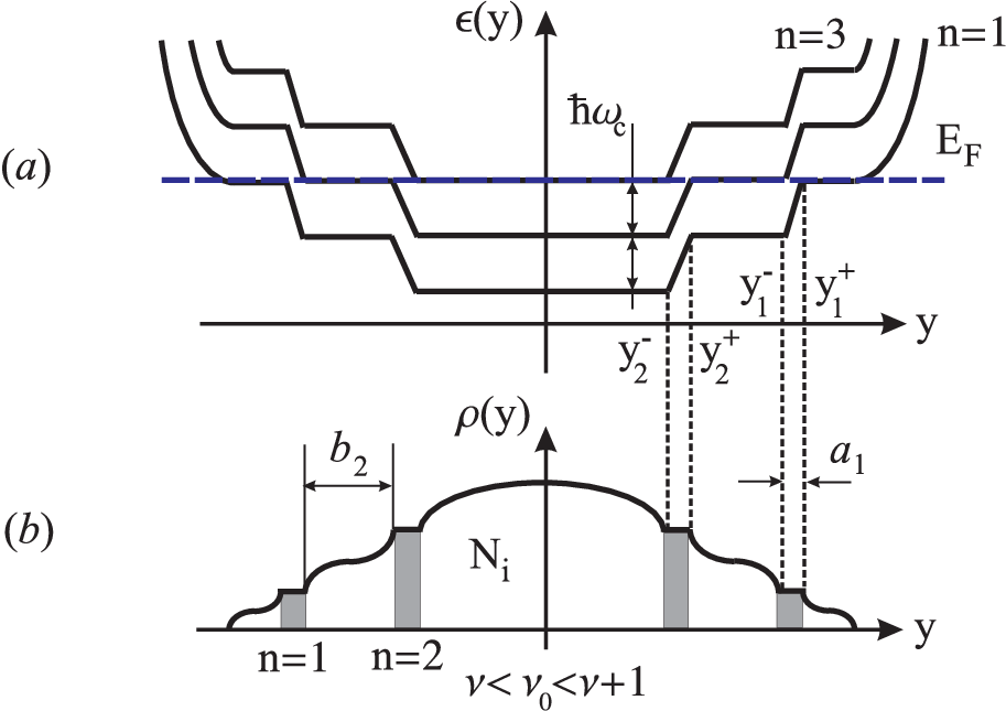
Refer to caption
Figure 6: (a) Fabry-Pérot interferometer with compressible island ii. The innermost edge channels ee are subject to backscattering at the QPCs; the remaining fT=ν−1f_{T}=\nu-1 right(rr)- and left(ll)- moving channels are fully transmitted; their role is in screening of the interaction between the electrons of the channel ee. Right- and left-moving channels are connected to reservoirs with different chemical potentials μη=e​Vη\mu_{\eta}=eV_{\eta}, η=±\eta=\pm. Here, the gate gg is depicted as a “plunger” gate. (b) Simple capacitance model, which uses geometry of the compressible regions. Right(rr)- and left(ll)-channels are each joined into one conductor with the widths brb_{r} and blb_{l}, respectively.
Refer to caption
Figure 7: The structure of the edge states in the FPI. Cut through the center of an interferometer cell: (a) Landau level energies as the function of vertical coordinate yy and (b) electron density ρ⁡(y)\rho(y) (see also Fig. 6). Besides ν\nu completely filled LLs, the central region can sustain a partially filled Landau level whose occupation NiN_{i} changes by tunneling. Here we denoted by ak=yk+−yk−a_{k}=y_{k}^{+}-y_{k}^{-} the width of the kk-th incompressible strip (shown by grey), which has the integer filling factor kk. Compressible regions (white) represent the regions with non-integer filling fraction and have the width bk=yk−1−−yk+b_{k}=y_{k-1}^{-}-y_{k}^{+}. The picture above corresponds to the case ν=2\nu=2.

Electrostatics of the FPI

In the framework of the above model, we treat the e-e interaction in the FPI by using the constant interaction model with mutual capacitances Cα​βC_{\alpha\beta} between four compressible regions — the interfering channel (ee); right- and left-moving fully transmitted channels (rr, ll); the compressible island (ii) — and the gate (gg). These capacitances are denoted by Ce​gC_{eg}, Ce​iC_{ei} etc. We assume a large capacitance between counter-propagating innermost channels — thus they share the same electrostatic potential φe\varphi_{e} — and also consider fT=ν−1f_{T}=\nu-1 right- and left-moving channels as joint conductors with potentials φr\varphi_{r} (φl\varphi_{l}). Defining a capacitance matrix C~\tilde{C} with elements C~α​α=∑γCα​γ+Cα​g\tilde{C}_{\alpha\alpha}=\sum_{\gamma}C_{\alpha\gamma}+C_{\alpha g}, and C~α​β=−Cα​β\tilde{C}_{\alpha\beta}=-C_{\alpha\beta} (α≠β\alpha\neq\beta), where Greek indices span the set {e,r,l,i}\{e,r,l,i\} and qα=−Cα​g​Vgq_{\alpha}=-C_{\alpha g}V_{g} is an offset charge on the α\alpha’s conductor, the electrostatic energy reads

E=12​∑α​β(Qα−qα)​(C~−1)α​β​(Qβ−qβ).\displaystyle E=\frac{1}{2}\sum_{\alpha\beta}\left(Q_{\alpha}-q_{\alpha}\right)\left(\tilde{C}^{-1}\right)_{\alpha\beta}\left(Q_{\beta}-q_{\beta}\right). (88)

Total charge Qi=e⁡(Ni+ν​ϕ/ϕ0)Q_{i}=e\left(N_{i}+\nu\phi/\phi_{0}\right) on the island is distributed on the highest partially filled Landau level (LL) and on ν\nu fully occupied underlying LLs (cf. Fig. 7). Single electron tunneling is possible between interfering channels (ee) and the island. We assume the rate of such tunneling process to be much smaller than all other energy scales in the problem, Γ≪ϵth\Gamma\ll\epsilon_{\rm th}, hence NiN_{i} is quantized and is fixed for given external parameters (ϕ\phi, VgV_{g}, μ±\mu_{\pm}).

The mutual capacitances Cα​βC_{\alpha\beta} can be estimated from geometrical considerations [22]. We regard the island as a disc of radius rr and represent the compressible edge channels as concentric rings of the width bαb_{\alpha} and diameter LL (here α=e,r,l\alpha=e,r,l) as depicted in Fig. 6 (b). The edge channels are assumed to be thin, bα≪Lb_{\alpha}\ll L. Therefore for estimation of capacitances we can neglect the difference between the radii of the island and those of edge channels, i.e. L≃π​r≃π​yk±L\simeq\pi r\simeq\pi y_{k}^{\pm}. A top gate, if present, is modeled by a plane situated at distance dd from the 2DEG. Since the size of FPI cell is much larger than dd, we treat Ci​gC_{ig}, Ce​gC_{eg} and Cr⁡(l)​gC_{r(l)g} as a parallel-plate capacitors and find an estimate

Ci​g≃ϵ​r24​d,Ce​g≃ϵ​L​be2​π​d,Cr​g≃ϵ​L​br4​π​d,C_{ig}\simeq\epsilon\frac{r^{2}}{4d},\qquad C_{eg}\simeq\epsilon\frac{Lb_{e}}{2\pi d},\qquad C_{rg}\simeq\epsilon\frac{Lb_{r}}{4\pi d}, (89)

where ϵ=12.6\epsilon=12.6 is the dielectric constant for GaAs. The estimate for edge-to-edge (Ce​rC_{er} and Ce​lC_{e\,l}) and edge-to-island (Ce​iC_{ei}) capacitances can be found as a mutual capacitance of two conducting rings. In the limit b≪ab\ll a we obtain with logarithmic accuracy [23]

Ce​r≃ϵ​L2​π2​ln⁡(be​brae​r2),Ce​i≃ϵ​rπ​ln⁡(r​beae​i2).C_{er}\simeq\frac{\epsilon L}{2\pi^{2}}\ln\left(\frac{b_{e}b_{r}}{a_{er}^{2}}\right),\quad C_{ei}\simeq\frac{\epsilon r}{\pi}\ln\left(\frac{rb_{e}}{a_{ei}^{2}}\right). (90)

Here br⁡(l)=∑kν−1bkb_{r(l)}=\sum_{k}^{\nu-1}b_{k} are the total widths of fully transmitted edge channels. Finding the mutual capacitance between a plunger gate and the island or the interfering edge channel is in general more difficult. Because of geometry, one can expect that Ci​gC_{ig} and Ce​gC_{eg} in this case will be substantially smaller than the above estimate (89) for the case of a top gate.

Let us now comment on the flux dependence of the electrostatic energy, Eq. (88). When the magnetic flux through the island is increased, δ​ϕ=π​r2​δ​B\delta\phi=\pi r^{2}\delta B , the LLs are squeezed and the charge on the island (for a fixed boundary yν−y_{\nu}^{-}) varies as δ​Qi=e​ν​δ​ϕ/ϕ0\delta Q_{i}=e\nu\,\delta\phi/\phi_{0}. A similar effect of magnetic field on charges Qe,r,lQ_{e,r,l} distributed on compressible circular strips is negligibly small because of the condition b≪rb\ll r. Indeed, for a typical variation δ​B\delta B, such that δ​ϕ/ϕ0∼1\delta\phi/\phi_{0}\sim 1, the corresponding modulation of these charges are

δ​Qe,r,le∼δ​ϕϕ0​(bπ​r)≪1,\frac{\delta Q_{e,r,l}}{e}\sim\frac{\delta\phi}{\phi_{0}}\left(\frac{b}{\pi r}\right)\ll 1, (91)

and we do not include them into Eq. (88).

4.2 Results

In this subsection we summarize our results and give their physical interpretation. The detailed derivation is presented in the next subsection. The qualitative behavior of the FPI crucially depends on the relative coupling strength of the interfering edge (ee) to the fully transmitted channels (ll, rr), to the island, and to the gate. The essential parameters are the number of transmitted channels ν∗\nu^{\ast} which screen the bare e-e interaction in the interfering channel — as we demonstrate in the section 4.3, one has ν∗≃1\nu^{\ast}\simeq 1 in the case of strong and ν∗≃ν\nu^{\ast}\simeq\nu in the case of weak inter-edge interaction — and the effective edge capacitance C¯e\bar{C}_{e} as defined below by Eq. (98). There are also two characteristic energy scales in our problem: (i) charging energy EC=e2/C¯eE_{C}=e^{2}/\bar{C}_{e}, or charge relaxation frequency ωC=(ν∗/π)​EC\omega_{C}=({\nu^{\ast}}/\pi)E_{C}; and (ii) the Thouless energy ϵth=τ−1=vF/L\epsilon_{\rm th}=\tau^{-1}={v_{F}}/L. A relation between these two parameters depends essentially on the geometry of the experiment (most importantly, on the geometry of the gates). We will assume that the condition ϵth≪ωC\epsilon_{\rm th}\ll\omega_{C} is always satisfied, which simplifies a lot our subsequent calculations and enables us to get analytical results. This appears to be a proper assumption for most of available experiments. In particular, the value of the Thouless energy that can be deduced from the experiment of the Harvard group is ϵth∼50​μ​V\epsilon_{\rm th}\sim 50\>\mu{\rm V} [26], whereas the charging energy is in the mV range [28].

4.2.1 Visibility, dephasing and the “lobe” structure

In the limit of weak backscattering, rj≪1r_{j}\ll 1, the differential conductance of the FPI, g=ginc+gABg=g_{\mathrm{inc}}+g_{\mathrm{AB}}, is the sum of incoherent and coherent contributions. The incoherent contribution is

ginc(V)=ν−R1∗(eV)−R2∗(eV),\displaystyle g_{\mathrm{inc}}(V)=\nu-R_{1\ast}(eV)-R_{2\ast}(eV), (92)

where Rj∗(eV)R_{j\ast}(eV) are the renormalized reflection coefficients (see Eq. (96) below). The dependence of the AB conductance on external parameters — the gate voltage VgV_{g}, the variation of the magnetic field Δ​B\Delta B and the bias VV — factorizes into

gAB​(μ+,μ−,ϕ,Vg)=g~​(V)​cos⁡[φAB​(Vg,Δ​B)].g_{\mathrm{AB}}(\mu_{+},\mu_{-},\phi,V_{g})=\tilde{g}(V)\cos[\varphi_{\rm AB}(V_{g},\Delta B)]. (93)

The AB phase φAB\varphi_{\rm AB} will be discussed in the details shortly. The amplitude of the oscillations is

g~(V)=e−τ/τφR12∗(eV) 2|cos(|eVτ|+π4​ν∗)|\displaystyle\tilde{g}(V)=e^{-\tau/\tau_{\varphi}}R_{12\ast}(eV)\ 2\left\lvert\cos\left(\lvert eV\tau\rvert+\frac{\pi}{4\nu^{\ast}}\right)\right\rvert (94)

with the nonequilibrium dephasing rate given by

τφ−1=|eV|(R1∗(eV)+R2∗(eV))2πsin2π2​ν∗.\displaystyle\tau_{\varphi}^{-1}=\lvert eV\rvert\left(R_{1\ast}(eV)+R_{2\ast}(eV)\right)\frac{2}{\pi}\sin^{2}\frac{\pi}{2\nu^{\ast}}. (95)

In Eqs. (92) and (94) we have introduced the renormalized reflection coefficients defined as

Rj∗(eV)=Rj|ωCe​V|1/ν∗eγ/ν∗Γ⁡(2−1/ν∗)=Rj∗(ϵth)|ϵthe​V|1/ν∗,R12∗(eV)=R12|ωCτ|1/2​ν∗|ωCe​V|1/2​ν∗21/2​ν∗​eγ/νΓ⁡(1−1/2​ν∗)=R12∗(ϵth)|ϵthe​V|1/2​ν∗.\displaystyle\begin{split}R_{j\ast}(eV)&=R_{j}\left\lvert\frac{\omega_{C}}{eV}\right\rvert^{1/\nu^{\ast}}\frac{e^{\gamma/\nu^{\ast}}}{\Gamma(2-1/\nu^{\ast})}=R_{j\ast}(\epsilon_{\rm th})\left\lvert\frac{\epsilon_{\rm th}}{eV}\right\rvert^{1/\nu^{\ast}},\\ R_{12\ast}(eV)&=R_{12}\ \lvert\omega_{C}\tau\rvert^{1/2\nu^{\ast}}\left\lvert\frac{\omega_{C}}{eV}\right\rvert^{1/2\nu^{\ast}}\frac{2^{1/2\nu^{\ast}}e^{\gamma/\nu}}{\Gamma(1-1/2\nu^{\ast})}=R_{12\ast}(\epsilon_{\rm th})\left\lvert\frac{\epsilon_{\rm th}}{eV}\right\rvert^{1/2\nu^{\ast}}.\end{split} (96)

Remarkably, in the last equation the amplitudes r1r_{1}, r2r_{2} do not renormalize separately, rather the renormalization operates non-locally. A similar result was found for FPIs in the fractional QHE regime in Ref. [49]. The relations (96) are valid for bias in the range ϵth≪e​V≪ωC\epsilon_{\rm th}\ll eV\ll\omega_{C}. The above renormalization comes from virtual electron-hole excitations (being a precursor of weak Coulomb blockade [24, 25]) and stops at e​V≃ϵtheV\simeq\epsilon_{\rm th}. On the contrary, the dephasing rate τφ−1\tau_{\varphi}^{-1} is caused by real e-h pairs excited by backscattered electrons and is proportional to the shot noise of the QPCs. There a simple linear dependence of the shot noise on voltage, which is valid in the absence of interaction, is modified because of the renormalization of reflection coefficients.

A functional dependence on bias in the conductance amplitude (94) stems from an oscillatory prefactor which has a characteristic scale π​ϵth\pi\epsilon_{\rm th}. As a consequence, the amplitude or, equivalently, the visibility v⁡(V)=|g~​(V)|/ginc​(V)v(V)=\lvert\tilde{g}(V)\rvert/g_{\mathrm{inc}}(V) vanishes for certain equidistantly distributed values of bias. The resulting characteristic “lobe” structure of visibility is shown in Fig. 8 and is in agreement with experiments reported in Refs. [27, 26].

Refer to caption
Refer to caption
Figure 8: Total differential conductance gg as a function of bias and magnetic flux (left panel), and visibility (right panel). Parameters are: ν∗=2\nu^{\ast}=2, ωC​τ=25\omega_{C}\tau=25, R1∗(ϵth)=R2∗(ϵth)=0.2R_{1\ast}(\epsilon_{\rm th})=R_{2\ast}(\epsilon_{\rm th})=0.2.

4.2.2 Aharonov-Bohm oscillations

In experiment one usually characterizes the FPI in terms of a pattern of its equilibrium conductance in the (B,Vg)(B,V_{g}) - plane, which is governed by AB phase. We have identified four different regimes where the behavior of AB oscillations is qualitatively different (see Table 1). In this table the parameter ν∗\nu^{\ast} — the effective number of transmitted channels which screen the Coulomb interaction in the interfering channel — depends on the relative strength of the inter-edge e-e interaction. To distinguish between the limits of weak and strong e-e interaction we compare an inter-channel interaction energy ∼e2/Ce​α\sim e^{2}/C_{e\alpha} (here α=r,l\alpha=r,l) with a screened by the gate charging energy of the interfering edge itself given by ∼e2/Cα​g∗\sim e^{2}/C^{*}_{\alpha g}. Here the edge-to-gate capacitance is effectively increased by the so-called “quantum capacitance”:

Cα​g∗=Cα​g+(ν−1)​τ​e2/(ℏ​π).C^{\ast}_{\alpha g}=C_{\alpha g}+(\nu-1)\tau e^{2}/(\hbar\pi). (97)

In the weak coupling limit one has Ce​α≫Cα​g∗C_{e\alpha}\gg C^{\ast}_{\alpha g}. In this case the electrostatic potentials on all edge channels (r,lr,l, and ee) are approximately equal to each other and we set ν∗≃ν\nu^{\ast}\simeq\nu. In the opposite strong coupling limit we have Ce​α≪Cα​g∗C_{e\alpha}\ll C^{\ast}_{\alpha g}. The potential φe\varphi_{e} here fluctuates independently of potentials on other edge channels (rr and ll), thus screening of e-e interaction by the latter channels is not effective and one gets ν∗≃1\nu^{\ast}\simeq 1.

Table 1: “Phase diagram” of the FPI, which discriminate between two Aharonov-Bohm (AB and AB*) and two Coulomb dominated (CD I and CD II) regimes.
Ce​α≫Cα​g∗C_{e\alpha}\gg C_{\alpha g}^{\ast} Ce​α≪Cα​g∗C_{e\alpha}\ll C_{\alpha g}^{\ast}
ν∗=ν\nu^{\ast}=\nu ν∗=1\nu^{\ast}=1
C¯e​i=Ce​i+Cr​i+Cl​i\bar{C}_{ei}=C_{ei}+C_{ri}+C_{li} C¯e​i=Ce​i\bar{C}_{ei}=C_{ei}
C¯e​g=Ce​g+Cr​g+Cl​g\bar{C}_{eg}=C_{eg}+C_{rg}+C_{lg} C¯e​g=Ce​g\bar{C}_{eg}=C_{eg}
C¯e​i≪Ci​g\bar{C}_{ei}\ll C_{ig} AB AB*
C¯e​i≫Ci​g\bar{C}_{ei}\gg C_{ig} CD II CD I

To make a distinction between the “Aharonov-Bohm” (AB) and “Coulomb-dominated” (CD) regimes we now define an effective edge-to-island capacitance C¯e​i\bar{C}_{ei} by the relation C¯e​i=Ce​i+Cr​i+Cl​i\bar{C}_{ei}=C_{ei}+C_{ri}+C_{li} in the weak coupling limit, i.e. at ν∗≃ν\nu^{\ast}\simeq\nu, and set it to be C¯e​i=Ce​i\bar{C}_{ei}=C_{ei} in the opposite case of strong coupling. Then the FPI falls into AB or CD regimes depending on a ratio C¯e​i/Ci​g\bar{C}_{ei}/C_{ig}, as it is shown in the Table 1. As one can see from Eqs. (89) and (90), for the device with a top gate the capacitance Ci​gC_{ig} scales like r2r^{2} when the FPI size grows, while C¯e​i\bar{C}_{ei} increases only as r​ln⁡rr\ln r. This suggests a simple rule of thumb: the AB regime occurs primary in large FPIs with a top gate (in experiment “large” means a cell area ∼\sim20μ​m2\mu{\rm m}^{2}). In this situation, i.e. at C¯e​i/Ci​g≪1\bar{C}_{ei}/C_{ig}\ll 1, fluctuations of charge on the island are screened by the gate electrode and do not affect the AB conductance. In the case of opposite ratio between the capacitances (C¯e​i/Ci​g≫1\bar{C}_{ei}/C_{ig}\gg 1), as one will see shortly, the AB conductance becomes linked to the Coulomb blockade on the compressible island. This explains a terminology choice — "Coulomb-dominated" — for the above regime.

For a device without the top gate a bare edge-to-gate capacitance Ce​gC_{eg} is due to only a plunger gate (see Fig. 6). Such gate is used to control the size of the interference loop and because of geometry Ce​gC_{eg} typically is very small, so that one has Ce​g∗≃(ν−1)​τ​e2/(ℏ​π)C^{\ast}_{eg}\simeq(\nu-1)\tau e^{2}/(\hbar\pi). In this case our first condition of weak versus strong inter-edge e-e coupling can be simplified. Defining the dimensionless coupling constant as

αν≡(ν−1)​e2ϵ​ℏ​vF\displaystyle\alpha_{\nu}\equiv\frac{(\nu-1)e^{2}}{\epsilon\hbar{v_{F}}}

and using the estimate (90) for capacitances Ce​rC_{er} and Ce​lC_{el} one obtains the crossover value

α∗∼12​π​ln⁡(be​brae​r2),\displaystyle\alpha^{\ast}\sim\frac{1}{2\pi}\ln\left(\frac{b_{e}b_{r}}{a_{er}^{2}}\right),

which sets the boundary between the weak and strong coupling regimes.

We name four regimes AB, AB*, CD I and CD II according to the Table 1 above which for the benefit of the reader lists the values of parameters ν∗\nu^{\ast}, C¯e​i\bar{C}_{ei} and C¯e​g\bar{C}_{eg}. The capacitance C¯e​g\bar{C}_{eg} here is defined in analogy to C¯e​i\bar{C}_{ei}. In addition to these effective edge-to-island and edge-to-gate capacitances we now define full island and edge capacitances as

C¯i=C¯e​i+Ci​g,C¯e=C¯e​g+C¯e​i​Ci​g/C¯i.\displaystyle\bar{C}_{i}=\bar{C}_{ei}+C_{ig},\quad\bar{C}_{e}=\bar{C}_{eg}+\bar{C}_{ei}C_{ig}/\bar{C}_{i}. (98)

Then the AB phase in Eq. (93) reads

φAB=2πϕ/ϕ0−2​πν∗C¯e​iC¯i(Ni∗+νϕ/ϕ0)+|e|ωC(2Vg−V+−V−)\displaystyle\varphi_{\rm AB}=2\pi\phi/\phi_{0}-\frac{2\pi}{\nu^{\ast}}\frac{\bar{C}_{ei}}{\bar{C}_{i}}(N_{i\ast}+\nu\phi/\phi_{0})+\frac{|e|}{\omega_{C}}\left(2V_{g}-V_{+}-V_{-}\right) (99)

with integer Ni∗N_{i\ast} minimizing the charging energy of the Coulomb island

Ei=e22​C¯i(Ni∗+νϕ/ϕ0−Ci​gVg/|e|)2,\displaystyle E_{i}=\frac{e^{2}}{2\bar{C}_{i}}(N_{i\ast}+\nu\phi/\phi_{0}-C_{ig}V_{g}/\lvert e\rvert)^{2}, (100)

and we have defined ωC=ν∗​EC/π\omega_{C}=\nu^{*}E_{C}/\pi and EC=e2/C¯eE_{C}=e^{2}/\bar{C}_{e}.

In Fig. 9 we show the conductance gAB​(ϕ,Vg)g_{\mathrm{AB}}(\phi,V_{g}) in the (BB,VgV_{g})–plane for three regimes: AB, CD-I and CD-II. The plots display significant differences. In particular, the lines of constant phase have a different slope in the AB and type-I CD regimes. The flux periodicity is also different in these two cases. The AB conductance in the case of type-II CD regime shows the “rhomb-like” pattern. The pattern of equilibrium conductance in the AB* case is the same as in the AB regime, provided one sets ν∗=1\nu^{*}=1.

Refer to caption
Refer to caption
Refer to caption
Figure 9: Aharonov-Bohm conductance: AB regime (left), ν∗=ν=2\nu^{\ast}=\nu=2, stripes of constant conductance have a negative slope, flux and gate voltage periods are Δ​ϕ=ϕ0\Delta\phi=\phi_{0} and Δ​Vg=ν​EC/|e|\Delta V_{g}=\nu E_{C}/\lvert e\rvert; type-I CD regime (middle), ν∗=1\nu^{\ast}=1, ν=3\nu=3, stripes of constant conductance have now a positive slope, flux and gate voltage periods are Δ​ϕ=ϕ0/(1−ν)\Delta\phi=\phi_{0}/(1-\nu) and Δ​Vg=EC/|e|\Delta V_{g}=E_{C}/\lvert e\rvert; type-I CD regime (right), ν∗=ν=2\nu^{\ast}=\nu=2, Ci​g/C¯e=0.6C_{ig}/\bar{C}_{e}=0.6, at fixed gate voltage VgV_{g} conductance depends discontinuously on flux — phase jumps occurs at every Δ​ϕ=ϕ0/ν\Delta\phi=\phi_{0}/\nu.

4.2.3 Discussion and comparison with experiment

Let us now discuss the physics which underlies the rich phenomenology of our rather simple model. To appreciate the role of interaction we consider first the non-interacting case, where the interfering channel couples neither to the fully transmitted ones nor to the island. Consider electron contributing to the tunneling current which is, say, incident from the left source and leaks into the left drain. It may tunnel either at the left or right QPC. The latter path is longer than the first by 2​L=2​vF​τ2L=2{v_{F}}\tau and encircles a magnetic flux ϕ\phi. Along this path the electron accumulates a dynamic (“Fabry-Pérot”) phase 2​ϵ​τ2\epsilon\tau (ϵ\epsilon is the energy of the electron) and a magnetic AB phase 2​π​ϕ/ϕ02\pi\phi/\phi_{0}. According to quantum mechanics, the current results from interference of both paths. Integration over all energies in the range μ−<ϵ<μ+\mu_{-}<\epsilon<\mu_{+} gives the back-scattering current

Ib=−e∫μ−μ+d​ϵ2​π|r1+e2​π​i​ϕ/ϕ0+2​i​ϵ​τr2|2=Iinc+IAB,I_{b}=-e\int_{\mu_{-}}^{\mu_{+}}\frac{\mathrm{d}\epsilon}{2\pi}\,\left\lvert r_{1}+e^{2\pi i\phi/\phi_{0}+2i\epsilon\tau}r_{2}\right\rvert^{2}=I_{\mathrm{inc}}+I_{\mathrm{AB}}, (101)

that we have split into incoherent and coherent contributions,

Iinc=−e22​π​V​(R1+R2),IAB=e2​π​2​R12τ​cos⁡[(μ++μ−)​τ−2​π​ϕ/ϕ0]​sin⁡[e​V​τ].I_{\mathrm{inc}}=-\frac{e^{2}}{2\pi}V(R_{1}+R_{2}),\quad I_{\mathrm{AB}}=\frac{e}{2\pi}\frac{2R_{12}}{\tau}\cos[(\mu_{+}+\mu_{-})\tau-2\pi\phi/\phi_{0}]\sin[eV\tau]. (102)

While the incoherent part of the current IincI_{\mathrm{inc}} is expected already on the classical level, IABI_{\mathrm{AB}} stems from interference and is sensitive to magnetic flux. The dynamic phase accumulated by an electron depends on its “absolute” energy ϵ\epsilon, and hence the current IABI_{\mathrm{AB}} depends on both chemical potentials μ+\mu_{+}, μ−\mu_{-}, but not just on their difference e​V=μ+−μ−eV=\mu_{+}-\mu_{-}. Clearly, the sum (μ++μ−\mu_{+}+\mu_{-}) enters only into the phase shift of the AB pattern, but not in the amplitude. However, this independence of the amplitude of oscillations on the bias does not in general hold for the differential conductance gABg_{\mathrm{AB}}. Specifically, when the differential conductance is calculated in the framework of the model of non-interacting electrons, the amplitude of the corresponding AB oscillations g~\tilde{g} does depend on the manner in which bias is applied.

Experimentally, the bias is applied asymmetrically: μ+=e​V\mu_{+}=eV, μ−=0\mu_{-}=0. The expected conductance then is

gAB=GQ−1​∂VIAB=−2​R12​cos⁡[2​e​V​τ+2​π​ϕ/ϕ0],\displaystyle g_{\mathrm{AB}}=G_{Q}^{-1}\partial_{V}I_{\mathrm{AB}}=-2R_{12}\cos[2eV\tau+2\pi\phi/\phi_{0}],

i.e. bias merely controls the phase shift of the AB oscillation pattern. The amplitude g~=−2​R12\tilde{g}=-2R_{12} is independent of bias. This clearly contradicts to our results presented above as well as to experimental observations.

The situation would change essentially if the bias were applied symmetrically: μ+=e​V/2\mu_{+}=eV/2, μ−=−eV/2\mu_{-}=-eV/2. Then the conductance would be

gAB=−2​R12​cos⁡[e​V​τ]​cos⁡[2​π​ϕ/ϕ0].g_{\mathrm{AB}}=-2R_{12}\cos[eV\tau]\cos[2\pi\phi/\phi_{0}]. (103)

Now, the amplitude would oscillate with bias on the scale π​ϵth\pi\epsilon_{\rm th}, yielding a visibility with a “lobe” structure. This result is apparently much more similar to our findings (albeit without dephasing and renormalization of R12R_{12}) as well to the experimental observations. On the basis of the similarity between Eq. (103) and the experimental observations it was conjectured in Ref. [28] that the electron-electron interaction effectively symmetrizes the bias even if the latter is applied asymmetrically.

To see how this works, assume that a charge within the interferometer cell produces a (for simplicity constant) self-consistent potential φ0\varphi_{0}. An electron which propagates in this potential during a time 2​τ2\tau accumulates the “electrostatic” AB phase −2​φ0​τ-2\varphi_{0}\tau. Hence, the dynamic phase would be 2​(ϵ−φ0)​τ2(\epsilon-\varphi_{0})\tau and instead of the bare chemical potentials the relative potentials (μ±−φ0)(\mu_{\pm}-\varphi_{0}) enter the result (102). Such a mean-field potential is indeed generated within our model. For instance, in the generic limit of large charging energy EC≫ϵthE_{C}\gg\epsilon_{\rm th} our calculations in the subsection 4.3 yield φ0≃(μ++μ−)/2\varphi_{0}\simeq(\mu_{+}+\mu_{-})/2 in the case of AB regime. Therefore without a need of any fine tuning, the bias is effectively symmetrized, which explains the appearance of the “lobe” structure.

The mean-field potential φ0\varphi_{0} on the compressible strip corresponding to the interfering edge channel is in general the function of applied chemical potentials μ±\mu_{\pm}, the gate voltage VgV_{g} and the magnetic flux ϕ\phi. The most general expression found in the subsection 4.3 reads

φ0(μ±,Vg,ϕ)=11+ωC​τ[eVg+μ++μ−2ωCτ+ECC¯e​iC¯i(Ni∗+νϕ/ϕ0)].\varphi_{0}(\mu_{\pm},V_{g},\phi)=\frac{1}{1+\omega_{C}\tau}\left[eV_{g}+\frac{\mu_{+}+\mu_{-}}{2}\omega_{C}\tau+E_{C}\frac{\bar{C}_{ei}}{\bar{C}_{i}}(N_{i\ast}+\nu\phi/\phi_{0})\right]. (104)

Here Ni∗N_{i\ast}, as before, provides the minimum for the Coulomb energy EiE_{i} of the island given by Eq. (100). If we introduce the electrochemical potential

φ~0=φ0−(μ++μ−)/2,\tilde{\varphi}_{0}=\varphi_{0}-(\mu_{+}+\mu_{-})/2, (105)

then the AB phase, given by Eq. (99), is equivalently represented by relation

φA​B​(μ±,Vg,ϕ)=2​π​ϕ/ϕ0−2​τ​φ~0​(μ±,Vg,ϕ).\varphi_{AB}(\mu_{\pm},V_{g},\phi)=2\pi\phi/\phi_{0}-2\tau\tilde{\varphi}_{0}(\mu_{\pm},V_{g},\phi). (106)

The first contribution here is the magnetic AB phase accumulated along a fixed reference loop with area A0A_{0}, i.e. ϕ=A0​δ​B\phi=A_{0}\delta B, with δ​B≪B\delta B\ll B being a weak modulation of magnetic field on top of the high field BB which drives the 2DEG into the QHE regime. Because of the condition b≪Lb\ll L (see Fig. 6 b) imposed in our model, and since a typical variation δ​B\delta B is such that ϕ\phi changes on a scale of a few flux quanta only, one can use any boundary yk±y_{k}^{\pm} to define A0A_{0}. For example, one can set A0=π​(yν+)2A_{0}=\pi(y_{\nu}^{+})^{2}. Let us further show, that the second “electrostatic” contribution (−2​τ​ϕ~0)(-2\tau\tilde{\phi}_{0}) to the phase φA​B\varphi_{AB} can be interpreted in terms of a motion of edge states which leads to the variation of a relevant FPI area when the magnetic field BB or gate voltage VgV_{g} are varied.

Refer to caption
Figure 10: When the boundaries of the compressible strip (white) separating incompressible regions (gray) with filling factors ν\nu and ν+1\nu+1 move towards the (ν+1)(\nu+1)-liquid (indicated by arrows), the latter shrinks while the ν\nu-liquid’s area grows: as the result the charge on the incompressible strip, defined by the boundaries yν+1−y_{\nu+1}^{-} and yν+y_{\nu}^{+}, decreases (in this figure hν<0h_{\nu}<0).

First, we note that in a stationary limit an imbalance of electron density per unit length on the interfering edge channel δ​ρe\delta\rho_{e} is related with the corresponding electrochemical potential (105) by a simple relation δρe=−φ~0/(2πvF)\delta\rho_{e}=-\tilde{\varphi}_{0}/(2\pi v_{F}), since (2​π​vF)−1(2\pi v_{F})^{-1} is just but the 1D thermodynamic density of states in our model. As it is always the case in QHE systems, this charge density can be translated into the variation hνh_{\nu} of the boundary between the compressible and incompressible strips (Fig. 10), δ​ρe=nL​hν\delta\rho_{e}=n_{L}h_{\nu}, where nL=B/ϕ0=(2​π​λB2)−1n_{L}=B/\phi_{0}=(2\pi\lambda_{B}^{2})^{-1} is the electron concentration on one completely filled LL, and we have assumed the fluctuations of inner and outer boundaries of the compressible strip to be the same, δ​yν+1+=δ​yν−=hν\delta y_{\nu+1}^{+}=\delta y_{\nu}^{-}=h_{\nu}. Therefore “electrostatic” part of the AB phase reads

−2​τ​φ~0=4​π​L​δ​ρe=4​π​nL​(L​hν)=2​π​(B/ϕ0)​δ​A.-2\tau\tilde{\varphi}_{0}=4\pi L\delta\rho_{e}=4\pi n_{L}(Lh_{\nu})=2\pi(B/{\phi_{0}})\delta A. (107)

Here δ​A=2​L​hν\delta A=2Lh_{\nu} is the change in area enclosed by interfering edge state. To recapitulate the logic, we have thus related the self-consistent electrostatic potential φ0\varphi_{0} to a variation of the FPI area. With these arguments at hand one can now rewrite Eqs. (104) and (106) in the equivalent form

ϕA​B=2​π​(A0​δ​B+B​δ​A)/ϕ0+const,\phi_{AB}=2\pi\bigl({A_{0}\delta B}+{B\delta A}\bigr)/{\phi_{0}}+{\rm const}\,, (108)

where the variation of area reads

δ​A=−1ν∗​C¯e​iC¯i​(ν​A0B​δ​B+ϕ0B​Δ​Ni)+|e|ωC​ϕ0π​B​δ​Vg.\delta A=-\frac{1}{\nu^{*}}\frac{\bar{C}_{ei}}{\bar{C}_{i}}\left(\nu\frac{A_{0}}{B}\,\delta B+\frac{\phi_{0}}{B}\,\Delta N_{i}\right)+\frac{|e|}{\omega_{C}}\frac{\phi_{0}}{\pi B}\,\delta V_{g}. (109)

In the last equation we have introduced an integer Δ​Ni\Delta N_{i} which is a deviation in excess number of electrons on the Coulomb island with respect to the excess charge corresponding to some initially chosen reference gate voltage VgV_{g}. We have also took into account the source-drain bias is small on a scale of the charging energy, |e|​V≪EC|e|V\ll E_{C}.

Let us now discuss our theory of the FPI in relation to the recent experiments by considering separately each of the four regimes in the Table 1. In the AB regime one has C¯e​i/Ci≪1\bar{C}_{ei}/C_{i}\ll 1, thus the coupling of the interfering edge to the Coulomb island is negligible and the area AA does not change with BB. The AB phase then simplifies to

φAB=2​π​ϕ/ϕ0+2​πν​|e|​VgEC,\varphi_{\rm AB}=2\pi\phi/\phi_{0}+\frac{2\pi}{\nu}\frac{\lvert e\rvert V_{g}}{E_{C}}, (110)

yielding the lines of constant phase with a negative slope (Fig. 9, left) and a magnetic field period Δ​B=ϕ0/A0\Delta B=\phi_{0}/A_{0} which is independent of ν\nu. The second term in the above equation describes a modulation in space of electron trajectory under variation of the gate voltage. If δ​Vg>0\delta V_{g}>0 then the interfering edge state moves outwards and thus encloses a larger flux as it is seen from Eq. (109). The AB regime was observed in large devices (cell area ∼\sim18μ​m2\mu{\rm m}^{2}) with a top gate [26, 28, 29], where the condition C¯e​i≪Cg​i\bar{C}_{ei}\ll C_{gi} is satisfied. In Ref. [28] it has been also found that magnetic field period Δ​B\Delta B is independent of BB but gate voltage periodicities (both top- and plunger- ones) scale as Δ​Vg∝1/B∝ν\Delta V_{g}\propto 1/B\propto\nu. These observation are consistent with our Eq. (110) if the charging energy EC=e2/C¯eE_{C}=e^{2}/{\bar{C}_{e}} is ν\nu - independent. It is so, provided the full edge capacitance C¯e≃Ce​g+C¯e​i\bar{C}_{e}\simeq C_{eg}+\bar{C}_{ei} stays approximately the same at each Hall plateau.

In the CD regime one has C¯e​i/Ci≃1\bar{C}_{ei}/C_{i}\simeq 1 and the area of the interfering loop shrinks with the magnetic field. This is because interfering edge is now electrostatically coupled to the charge Qi=e⁡(Ni+ν​ϕ/ϕ0)Q_{i}=e(N_{i}+\nu\phi/\phi_{0}) on the Coulomb island, which has explicit dependence on flux. The AB phase in this regime reads

φAB=2​π​(1−ν/ν∗)​ϕ/ϕ0−2​πν∗​Ni+2​πν∗​|e|​VgEC,\displaystyle\varphi_{\rm AB}=2\pi(1-\nu/\nu^{*})\phi/\phi_{0}-\frac{2\pi}{\nu^{*}}N_{i}+\frac{2\pi}{\nu^{*}}\frac{\lvert e\rvert V_{g}}{E_{C}},

In the type-II CD regime ν∗≃ν\nu^{*}\simeq\nu and at fixed VgV_{g} the AB phase stays piecewise constant when the magnetic field is varied. The dependence of phase on BB exclusively enters via NiN_{i}. Indeed, as it follows from Eq. (109) the shrinkage of the interfering loop in this case, δ​A=−(A0/B)​δ​B\delta A=-(A_{0}/B)\delta B, exactly compensates a change in magnetic phase φ=A0​δ​B\varphi=A_{0}\delta B. When the FPI is brought close to a charge degeneracy point of the island by varying VgV_{g} or BB, electron tunneling becomes possible between the droplet and interfering channels (i.e. Δ​Ni=±1\Delta N_{i}=\pm 1) resulting in abrupt change of AA. This creates a phase lapse (or jump) ΔϕA​B=±2π/ν\Delta\phi_{AB}=\pm 2\pi/\nu giving rise to the “rhomb-like” pattern shown in Fig. 9 (middle) at ν≥2\nu\geq 2.

In the type-I CD regime ν∗≃1\nu^{*}\simeq 1 and a change in AB phase caused by area shrinkage when rising BB overcompensates the magnetic AB phase, since now δ​A=−ν⁡(A0/B)​δ​B\delta A=-\nu(A_{0}/B)\delta B. Counterintuitively, the phase decreases for increasing the magnetic field. At the same time, whenever an electron tunnels into the island from the interfering edge channel (ee), the boundary of this edge state contracts so as to expel exactly one flux quantum from the AB loop. The phase lapse, being equal to Δ​ϕA​B=(−2​π)\Delta\phi_{AB}=(-2\pi) in this tunneling process, is therefore invisible in the interference conductance. As the result, one has the diagonal stripe pattern with lines of constant phase having positive slope (Fig. 9, right). The periods are Δ​B=ϕ0/(fT​A)\Delta B=\phi_{0}/(f_{T}A) and Δ​Vg=e/(Ce​g+Cg​i)\Delta V_{g}=e/(C_{eg}+C_{gi}), with fT=ν−1f_{T}=\nu-1 being the number of fully transmitted edge channels (note, that at ν=1\nu=1 the lines of constant phase are vertical).

In the limit of weak backscattering at QPCs, the Coulomb-dominated regime has been observed in Ref. [29]. In this work measurements were performed with the set of edge state configurations (including fractional fillings), classified by bulk filling fbf_{b} and number fTf_{T} of fully transmitted edges. We focus on the results obtained with a 4.4 μ​m2\mu{\rm m}^{2}-device without a top (but with plunger-) gate. They indicate that interaction plays a major role (i.e. CD-I and CD-II regimes). For integer fbf_{b} and fT=fb−1f_{T}=f_{b}-1 the results coincide with our Fig. 9 (right), including the period in magnetic field which scales as Δ​B∝1/fT\Delta B\propto 1/f_{T}. The gate period in Ref. [29] was found to be weakly increasing with fTf_{T}. We can explain this dependence if one assumes that the full edge capacitance, which equals to C¯e=Cg​i+Ce​g\bar{C}_{e}=C_{gi}+C_{eg} in the CD-I regime, decreases with fTf_{T}, since a mutual coupling of the plunger-gate to the inner interfering edge channel (Ce​gC_{eg}) becomes less efficient at high ν\nu. Quite “exotic” behavior was observed for more than one number of channels trapped in the interferometer cell. In case of fb=4f_{b}=4 and fT=1f_{T}=1 experimental findings resemble very much Fig. 9 (middle) corresponding to our CD-II regime. In such setting one fully transmitted and one partially reflected edge channel can be described by our model with ν=2\nu=2 assuming that other two inner trapped channels play a role of a compressible island, where the excess charge is quantized.

Non-equilibrium transport measurements in the FPIs in the AB regime have been performed in Refs. [26, 27]. Their main findings can be summarized as follows: (i) the dependence of AB conductance versus BB and the bias VV factorizes into a product of two terms yielding a “checkerboard" pattern in the (δ​B,V)(\delta B,V)-plane (cf. Fig. 8, left); (ii) the scale of the “lobe"-structure is set by ϵTh∼vD/L\epsilon_{\rm Th}\sim v_{D}/L; (iii) a visibility decay with bias is stronger at higher magnetic fields. Results of our theory, Eqs. (93) - (96), are in full accord with these observations. In particular, a suppression of visibility in our model at |rj|2≪1|r_{j}|^{2}\ll 1 is mainly due to a power-law decay with the negative exponent (−1/2ν∗)(-1/2\nu^{*}). Since in the AB regime ν∗=ν∝1/B\nu^{*}=\nu\propto 1/B, this decay is stronger in case of a small number of edge channels, i.e. at higher BB, in agreement with Ref. [26].

It is interesting to note, that our theory predicts a fourth regime (AB∗, see Table 1). It is characterized by the same equilibrium conductance pattern as the AB regime (Fig. 9, left), but in contrast to the latter, the power-law decay of the visibility oscillations corresponds to ν∗=1\nu^{\ast}=1, and thus is independent of BB. Such a behavior of the FPI has not yet been observed in the experiment.

Closing this section we have to mention that a crossover from the AB to the type-I CD regime (in our) terminology has been recently discussed in details in Ref. [51]. We note that our capacitance model is very similar in spirit to the one used in that paper. However, the important difference is that our approach takes explicitly into account quantum corrections to classical geometrical capacitances, given by Eq. (97). As the result we obtain the extra type-II CD regime which may arise because of screening of Coulomb interaction by the fully transmitted edge channels.

4.3 Calculations

We show here how to derive the above results using the formalism developed in Sect. 2. For simplicity we assume all edge channels to have the same length LL and same velocity |vμ|=vF\lvert v_{\mu}\rvert={v_{F}} (with vμ>0v_{\mu}>0 in right-moving channels and vμ<0v_{\mu}<0 in left-moving ones). Consequently, all flight times τ=L/vF\tau=L/{v_{F}} are the same. Further, the scatterer 1 has a coordinate x1x^{1} and scatterer 2 has the coordinate x2=x1+Lx^{2}=x^{1}+L for each of the edges, see Fig. 11.

Refer to caption
Figure 11: Network model of the FPI.

We remind that two characteristic energy scales play an important role in our analysis, namely, Thouless energy ϵth=τ−1\epsilon_{\rm th}=\tau^{-1} and charging energy EC=e2/C¯eE_{C}=e^{2}/\bar{C}_{e} (or charge relaxation frequency ωC=ν∗π​EC\omega_{C}=\frac{\nu^{\ast}}{\pi}E_{C}), see Sec. sec:FPI-results. As has been discussed there, we will assume that the charging energy is much higher than the Thouless energy, and will consider the range of voltages intermediate between these two scales, ωC≫|e​V|≫ϵth\omega_{C}\gg\lvert eV\rvert\gg\epsilon_{\rm th}.

4.3.1 Electrostatic Action

Our network consists of ν\nu right-moving and ν\nu left-moving chiral channels which we label with index μ\mu, see Fig. 11. The innermost right-moving channel (μ=+\mu=+) is coupled to the innermost left-moving channel (μ=−\mu=-) by two scatterers i=1,2i=1,2 with 2×22\times 2-scattering matrices sis^{i}. The remaining chiral channels (right-moving ones labeled μ=r​1,…,r⁡(ν−1)\mu=r1,\ldots,r(\nu-1), left-moving ones by μ=l​1,…,l⁡(ν−1)\mu=l1,\ldots,l(\nu-1)) connect sources to drains without any possibility of tunneling.

Interaction is taken into account by the electrostatic model (88) described in the beginning. For simplicity we assumed that electrostatic coupling between all fully transmitted right-moving channels (μ=r​1,…,r⁡(ν−1)\mu=r1,\ldots,r(\nu-1)) is strong such that they share a common electrostatic potential VrV_{r}. This enables us to merge them into one conductor (labeled α=r\alpha=r). We proceeded in the same way with the fully transmitted left-moving ones (μ=l​1,…,l⁡(ν−1)\mu=l1,\ldots,l(\nu-1) are now merged into α=l\alpha=l) and the two innermost channels (μ=+,−\mu=+,- are merged into α=e\alpha=e). This reduces the number of charge degrees of freedom characterizing the edge channels down to three:

Qe=∫d​x​ψ¯+​ψ++∫d​x​ψ¯−​ψ−,Qr=∑κ=1ν−1∫d​x​ψ¯r​κ​ψr​κ,Ql=∑κ=1ν−1∫d​x​ψ¯l​κ​ψl​κ.\displaystyle Q_{e}=\int\!\!\mathrm{d}x\,\bar{\psi}_{+}\psi_{+}+\int\!\!\mathrm{d}x\,\bar{\psi}_{-}\psi_{-},\quad Q_{r}=\sum_{\kappa=1}^{\nu-1}\int\!\!\mathrm{d}x\,\bar{\psi}_{r\kappa}\psi_{r\kappa},\quad Q_{l}=\sum_{\kappa=1}^{\nu-1}\int\!\!\mathrm{d}x\,\bar{\psi}_{l\kappa}\psi_{l\kappa}.

As a fourth conducting element, we introduce a central compressible island with total charge Qi=e⁡(Ni+ν​ϕ/ϕ0)Q_{i}=e(N_{i}+\nu\phi/\phi_{0}). While the second contribution, the charge in the ν\nu fully occupied LLs of the central region, is fixed by external parameters, the occupation NiN_{i} of the partially filled LL of the island is an (integer) degree of freedom to begin with. Since it is assumed to fluctuate via very slow tunneling, Γ≪ϵth\Gamma\ll\epsilon_{\rm th}, we will, however, treat it in a mean-field approximation.

The fermionic action we start with reads as follows

𝒜0[ψ,ψ¯,Ni]=∑μ∫𝒞dtdxψ¯μ(i∂t+ivμ∂x)ψμ−12∑α​β(Qα−qα)(C~−1)α​β(Qβ−qβ),\displaystyle\mathcal{A}_{0}[\psi,\bar{\psi},N_{i}]=\sum_{\mu}\,\int_{\mathcal{C}}\mathrm{d}t\mathrm{d}x\,\bar{\psi}_{\mu}\left(i\partial_{t}+iv_{\mu}\partial_{x}\right)\psi_{\mu}-\frac{1}{2}\sum_{\alpha\beta}\left(Q_{\alpha}-q_{\alpha}\right)\left(\tilde{C}^{-1}\right)_{\alpha\beta}\left(Q_{\beta}-q_{\beta}\right)\,,

where the first sum extends over the 2​ν2\nu chiral channels μ=r​1,…,r⁡(ν−1),l​1,…,l⁡(ν−1),+,−\mu=r1,\ldots,r(\nu-1),l1,\ldots,l(\nu-1),+,- and the second one over the 4 conductors α,β=e,r,l,i\alpha,\beta=e,r,l,i. The electrostatic part of 𝒜0​[ψ,ψ¯,Ni]\mathcal{A}_{0}[\psi,\bar{\psi},N_{i}] is, of course, a direct consequence of (88) and we refer to the corresponding section for definitions of qαq_{\alpha} and C~\tilde{C}. Charges QαQ_{\alpha} are, of course, dynamic, i.e. time-dependent, quantities, but for the sake of readability we leave time-dependence implicit (as we did with time integration in the above electrostatic action).

Our interest lies in interference effects which manifest themselves in tunneling corrections to current. Tunneling phases respond only to the Hubbard-Stratonovich field φ=e​Ve\varphi=eV_{e} on the interfering edges (note that the electrostatic merging of channels μ=+,−\mu=+,- allows us to use just one field φ=φ+=φ−\varphi=\varphi_{+}=\varphi_{-}). The short-term goal of the present section is to integrate out all other degrees of freedom.

Potentials Vc=(Ve,Vr,Vl)tV_{c}=(V_{e},V_{r},V_{l})^{t}:

First, we decouple the quadratic charge terms via a (multidimensional) Hubbard-Stratonovich transformation, thereby (re)introducing the potentials VαV_{\alpha} on the conductors. Since we do not need the potential ViV_{i} on the island, we single out the island degrees of freedom beforehand, writing

C~−1=(pc​cpc​ipi​cpi​i),Vc​i=pc​i​(Qi−qi).\displaystyle\tilde{C}^{-1}=\begin{pmatrix}p_{cc}&p_{ci}\\ p_{ic}&p_{ii}\end{pmatrix},\ V_{ci}=p_{ci}(Q_{i}-q_{i}). (111)

The index cc refers to the 3 indices ee, rr, ll, that means pc​cp_{cc}, pc​i=pi​ctp_{ci}=p_{ic}^{t}, pi​ip_{ii} are 3×33\times 3-, 3×13\times 1-, and 1×11\times 1-matrices. With that the action reads

𝒜int​[ψ,ψ¯,Ni]\displaystyle\mathcal{A}_{\mathrm{int}}[\psi,\bar{\psi},N_{i}] =−12​(Qi−qi)2​pi​i−12​(Qc−qc)t​pc​c​(Qc−qc)−Vc​it​(Qc−qc)\displaystyle=-\frac{1}{2}(Q_{i}-q_{i})^{2}p_{ii}-\frac{1}{2}(Q_{c}-q_{c})^{t}p_{cc}(Q_{c}-q_{c})-V_{ci}^{t}(Q_{c}-q_{c})

and becomes upon Hubbard-Stratonovich decoupling:

𝒜int​[ψ,ψ¯,Vc,Ni]−12​(Qi−qi)2​pi​i+12​(Vc−Vc​i)t​pc​c−1​(Vc−Vc​i)−Vct​(Qc−qc)\displaystyle\mathcal{A}_{\mathrm{int}}[\psi,\bar{\psi},V_{c},N_{i}]-\frac{1}{2}(Q_{i}-q_{i})^{2}p_{ii}+\frac{1}{2}(V_{c}-V_{ci})^{t}p_{cc}^{-1}(V_{c}-V_{ci})-V_{c}^{t}(Q_{c}-q_{c})
with ​Vc=(Ve,Vr,Vl)t.\displaystyle\text{with }V_{c}=(V_{e},V_{r},V_{l})^{t}.
Integrating out QeQ_{e}, QrQ_{r}, QlQ_{l}:

Next, we integrate out the charges QeQ_{e}, QrQ_{r}, QlQ_{l}. As explained in Sect. 2.1 and 2.2 charges and potentials are decoupled by a gauge transformation (2) which generates a tunneling term 𝒜t\mathcal{A}_{t} (see below) and, according to the Dzyaloshinskii-Larkin theorem, quadratic and linear (in voltages) terms Vα2​SαV_{\alpha}^{2}S_{\alpha} and Q¯α​Vα\bar{Q}_{\alpha}V_{\alpha}. The former is given by the polarization operators (10) and amounts for screening, thus an “enhancement” of the capacitances (in fact, the capacitances become complex, “Keldysh”- and energy-dependent, but in the static limit the corrections are indeed positive). Then the retarded/advanced components of the “screening capacitances” read

Sαr/a​(ω)=−e2∑κ=1ν−1∫dξ1dξ2Πα​κr/a(ω,ξ1,ξ2)=±i(ν−1)e21−e±i​ω​τ2​π​ω,α=r,l,Ser/a​(ω)=−e2∑μ=±∫dξ1dξ2Πμr/a(ω,ξ1,ξ2)=±i2e21−e±i​ω​τ2​π​ω.\displaystyle\begin{split}S^{r/a}_{\alpha}(\omega)&=-e^{2}\sum_{\kappa=1}^{\nu-1}\int\!\mathrm{d}\xi_{1}\mathrm{d}\xi_{2}\,\Pi_{\alpha\kappa}^{r/a}(\omega,\xi_{1},\xi_{2})=\pm i(\nu-1)e^{2}\frac{1-e^{\pm i\omega\tau}}{2\pi\omega},\quad\alpha=r,l,\\ S^{r/a}_{e}(\omega)&=-e^{2}\sum_{\mu=\pm}\int\!\mathrm{d}\xi_{1}\mathrm{d}\xi_{2}\,\Pi_{\mu}^{r/a}(\omega,\xi_{1},\xi_{2})=\pm i2e^{2}\frac{1-e^{\pm i\omega\tau}}{2\pi\omega}.\end{split} (112)

Charges injected from the reservoirs due to nonequilibrium boundary conditions (in excess of the equilibrium charge which is canceled by the positive background charge) are

Q¯r=(ν−1)​e​μ+​τ2​π,Q¯l=(ν−1)​e​μ−​τ2​π,Q¯e=e​(μ++μ−)​τ2​π.\displaystyle\bar{Q}_{r}=(\nu-1)e\frac{\mu_{+}\tau}{2\pi},\quad\bar{Q}_{l}=(\nu-1)e\frac{\mu_{-}\tau}{2\pi},\quad\bar{Q}_{e}=e\frac{(\mu_{+}+\mu_{-})\tau}{2\pi}. (113)

We collect them in the diagonal matrix S=diag⁡(Se,Sr,Sl)S=\mathrm{diag}\,(S_{e},S_{r},S_{l}) and the vector Q¯c=(Q¯e,Q¯r,Q¯l)t\bar{Q}_{c}=(\bar{Q}_{e},\bar{Q}_{r},\bar{Q}_{l})^{t}. Subsequent elimination of charge degrees of freedom transforms 𝒜int​[ψ,ψ¯,Vc,Ni]\mathcal{A}_{\mathrm{int}}[\psi,\bar{\psi},V_{c},N_{i}] into

𝒜0​[Vc,Ni]=−12​p¯i​i​(Qi−qi)2+12​Vct​(pc​c−1+S)​Vc−Vct​(Q¯c−qc+pc​c−1​Vc​i)\displaystyle\mathcal{A}_{0}[V_{c},N_{i}]=-\frac{1}{2}\bar{p}_{ii}(Q_{i}-q_{i})^{2}+\frac{1}{2}V_{c}^{t}(p_{cc}^{-1}+S)V_{c}-V_{c}^{t}(\bar{Q}_{c}-q_{c}+p_{cc}^{-1}V_{ci})
with ​p¯i​i=pi​i−pi​c​pc​c−1​pc​i.\displaystyle\text{with }\bar{p}_{ii}=p_{ii}-p_{ic}p_{cc}^{-1}p_{ci}. (114)
Integrating out VrV_{r}, VlV_{l}:

The final, and somewhat cumbersome step is to integrate out the voltages VrV_{r}, VlV_{l}. In order to do that we again split the degrees of freedom, writing

pc​c−1=(ce​ece​tct​ect​t),S=(SeSt),\displaystyle p_{cc}^{-1}=\begin{pmatrix}c_{ee}&c_{et}\\ c_{te}&c_{tt}\end{pmatrix},\quad S=\begin{pmatrix}S_{e}&\\ &S_{t}\end{pmatrix}, (115)

where the index tt refers to the 2 indices rr, ll, and ce​ec_{ee}, ce​t=ct​etc_{et}=c_{te}^{t}, ct​tc_{tt} are corresponding 1×11\times 1-, 1×21\times 2-, and 2×22\times 2-matrices. The action then reads

𝒜0​[Vc,Ni]=\displaystyle\mathcal{A}_{0}[V_{c},N_{i}]= −12​p¯i​i​(Qi−qi)2+12​(ce​e+Se)​Ve2−Ve​(Q¯e−qe+ce​e​Ve​i+ce​t​Vt​i)\displaystyle-\frac{1}{2}\bar{p}_{ii}(Q_{i}-q_{i})^{2}+\frac{1}{2}(c_{ee}+S_{e})V^{2}_{e}-V_{e}(\bar{Q}_{e}-q_{e}+c_{ee}V_{ei}+c_{et}V_{ti})
+12​Vtt​(ct​t+St)​Vt−Vtt​(Q¯t−qt+ct​e​Ve​i+ct​t​Vt​i−ct​e​Ve).\displaystyle+\frac{1}{2}V_{t}^{t}(c_{tt}+S_{t})V_{t}-V_{t}^{t}(\bar{Q}_{t}-q_{t}+c_{te}V_{ei}+c_{tt}V_{ti}-c_{te}V_{e}).

Performing the Gaussian integration over VrV_{r}, VlV_{l} is a straightforward, albeit cumbersome calculation which in the end yields,

𝒜0​[Ve,Ni]=−12​C¯i​(Qi−qi)2−(Q¯t−qt)t​p¯t​i​(Qi−qi)+12​C¯e∗​Ve2−Ve​(Q¯e−qe+xe​t​(Q¯t−qt)+xe​i​(Qi−qi))\mathcal{A}_{0}[V_{e},N_{i}]=-\frac{1}{2\bar{C}_{i}}(Q_{i}-q_{i})^{2}-(\bar{Q}_{t}-q_{t})^{t}\bar{p}_{ti}(Q_{i}-q_{i})+\frac{1}{2}\bar{C}^{\ast}_{e}V_{e}^{2}-V_{e}(\bar{Q}_{e}-q_{e}+x_{et}(\bar{Q}_{t}-q_{t})+x_{ei}(Q_{i}-q_{i})) (116)

where we have introduced the effective capacitances and coupling strengths

C¯i−1\displaystyle\bar{C}_{i}^{-1} ≡pi​i−pi​c​pc​c−1​pc​i+(pi​e​ce​t+pi​t​ct​t)​(ct​t+St)−1​(ct​e​pe​i+ct​t​pt​i),\displaystyle\equiv p_{ii}-p_{ic}p_{cc}^{-1}p_{ci}+(p_{ie}c_{et}+p_{it}c_{tt})(c_{tt}+S_{t})^{-1}(c_{te}p_{ei}+c_{tt}p_{ti}),
C¯e∗\displaystyle\bar{C}^{\ast}_{e} ≡ce​e+Se−ce​t(ct​t+St)−1ct​e,C¯e≡C¯e∗|Se=Sr=Sl=0\displaystyle\equiv c_{ee}+S_{e}-c_{et}(c_{tt}+S_{t})^{-1}c_{te},\quad\bar{C}_{e}\equiv\bar{C}_{e}^{\ast}\Big\rvert_{S_{e}=S_{r}=S_{l}=0}
xe​t\displaystyle x_{et} ≡−ce​t​(ct​t+St)−1,\displaystyle\equiv-c_{et}(c_{tt}+S_{t})^{-1},
xe​i\displaystyle x_{ei} ≡ce​e​pe​i+ce​t​pt​i−ce​t​(ct​t+St)−1​(ct​e​pe​i+ct​t​pt​i),\displaystyle\equiv c_{ee}p_{ei}+c_{et}p_{ti}-c_{et}(c_{tt}+S_{t})^{-1}(c_{te}p_{ei}+c_{tt}p_{ti}),
p¯t​i\displaystyle\bar{p}_{ti} ≡(ct​t+St)−1​(ct​e​pe​i+ct​t​pt​i).\displaystyle\equiv(c_{tt}+S_{t})^{-1}(c_{te}p_{ei}+c_{tt}p_{ti}).
Regimes ABI, CDI, CDII:

In the limits of very strong, i.e.

Cα​e≪Ce​g+Se,\displaystyle C_{\alpha e}\ll C_{eg}+S_{e},

and very weak, i.e.

Cα​e\displaystyle C_{\alpha e} ≫(Cα​g+Sα)2Ce​g+Cr​g+Cl​g+Se+Sr+Sl,\displaystyle\gg\frac{(C_{\alpha g}+S_{\alpha})^{2}}{C_{eg}+C_{rg}+C_{lg}+S_{e}+S_{r}+S_{l}},

coupling between fully transmitted edges α=r,l\alpha=r,l and interfering edge ee the expressions simplify to

Strong coupling Weak coupling
C¯i\bar{C}_{i} Ce​i+Ci​gC_{ei}+C_{ig} Ce​i+Cr​i+Cl​i+Ci​gC_{ei}+C_{ri}+C_{li}+C_{ig}
C¯e∗\bar{C}_{e}^{\ast} Ce​g+Se+Ci​g−Ci​g2/C¯iC_{eg}+S_{e}+C_{ig}-C_{ig}^{2}/\bar{C}_{i} Ce​g+Cr​g+Cl​g+Se+Sl+Sr+Ci​g−Ci​g2/C¯iC_{eg}+C_{rg}+C_{lg}+S_{e}+S_{l}+S_{r}+C_{ig}-C_{ig}^{2}/\bar{C}_{i}
xe​tx_{et} (00)\begin{pmatrix}0&0\end{pmatrix} (11)\begin{pmatrix}1&1\end{pmatrix}
xe​ix_{ei} Ce​i/C¯iC_{ei}/\bar{C}_{i} (Ce​i+Cr​i+Cl​i)/C¯i(C_{ei}+C_{ri}+C_{li})/\bar{C}_{i}
p¯t​i\bar{p}_{ti} 0 0,

and using Eqs. (111)-(115), the action becomes

𝒜0​[φ,Ni]=12​∫𝒞d​t​d​t′​φ​(t)​V−1​(t−t′)​φ​(t′)−∫𝒞d​t​φ​(t)​N0​(t)−12​C¯i​(Qi−qi)2\displaystyle\mathcal{A}_{0}[\varphi,N_{i}]=\frac{1}{2}\int_{\mathcal{C}}\mathrm{d}t\,\mathrm{d}t^{\prime}\,\varphi(t)V^{-1}(t-t^{\prime})\varphi(t^{\prime})-\int_{\mathcal{C}}\mathrm{d}t\,\varphi(t)N_{0}(t)-\frac{1}{2\bar{C}_{i}}(Q_{i}-q_{i})^{2} (117)
withVr/a​(ω)=EC​ωω±i​ωC​(1−e±i​ω​τ),N0≡ν∗π​μ++μ−2​τ−|e|​VgEC−C¯e​iC¯i​Qi/|e|\displaystyle\begin{split}\text{with}\quad V^{r/a}(\omega)&=E_{C}\frac{\omega}{\omega\pm i\omega_{C}(1-e^{\pm i\omega\tau})},\\ N_{0}&\equiv\frac{\nu^{\ast}}{\pi}\frac{\mu_{+}+\mu_{-}}{2}\tau-\frac{\lvert e\rvert V_{g}}{E_{C}}-\frac{\bar{C}_{ei}}{\bar{C}_{i}}Q_{i}/\lvert e\rvert\end{split} (118)

Here C¯i\bar{C}_{i}, C¯e\bar{C}_{e}, C¯e​g\bar{C}_{eg}, C¯e​i\bar{C}_{ei}, and ν∗\nu^{\ast} are given in Sect. 4.2.2 (Eq. (98) and table above).

4.3.2 Tunneling Action

To construct the tunneling action 𝒜t​[φ]\mathcal{A}_{t}[\varphi] in lowest order we use Eq. (20) which makes it necessary to identify the paths (i​j;μ​ν)(ij;\mu\nu). Only the innermost chiral channels μ,ν=±\mu,\nu=\pm allow for tunneling between each other at scatterers i,j=1,2i,j=1,2 which gives 4 classes: (11;+−)(11;+-), (22;+−)(22;+-), (12;+−)(12;+-), and (21;+−)(21;+-). Classical phases are accumulated due to magnetic flux ϕ\phi:

Δϕ11+⁣−=Δϕ22+⁣−=0,Δϕ12+⁣−=−Δϕ21+⁣−=−2πϕ/ϕ0.\displaystyle\Delta\phi^{11}_{+-}=\Delta\phi^{22}_{+-}=0,\quad\Delta\phi^{12}_{+-}=-\Delta\phi^{21}_{+-}=-2\pi\phi/\phi_{0}.

At zero temperature the distribution functions read f±≷​(t)=e−i​μ±​t​f0≷​(t)f^{\gtrless}_{\pm}(t)=e^{-i\mu_{\pm}t}f_{0}^{\gtrless}(t) with Fermi distribution function f0≷​(t)f_{0}^{\gtrless}(t). Writing for short ri≡s−⁣+ir_{i}\equiv s^{i}_{-+}, χ≡χ+−χ−\chi\equiv\chi_{+}-\chi_{-}, ϵi​j=ϵi​j​3\epsilon_{ij}=\epsilon_{ij3} (the right-hand side being the 3-dimensional Levi-Civita symbol), and Πi​j≡Πij;+−\Pi_{ij}\equiv\Pi_{ij;+-} we obtain the tunneling operators (22, 23)

Πi​j≷​(t)\displaystyle\Pi_{ij}^{\gtrless}(t) =−ri​r¯j​e±i​χ​e−i​ϵi​j​[2​π​ϕ/ϕ0+(μ++μ−)​τ]​e−i​e​V​t​f0≷​(t+ϵi​j​τ)​f0≶​(t−ϵi​j​τ),\displaystyle=-r_{i}\bar{r}_{j}\ e^{\pm i\chi}\ e^{-i\epsilon_{ij}\left[2\pi\phi/\phi_{0}+(\mu_{+}+\mu_{-})\tau\right]}\ e^{-ieVt}f_{0}^{\gtrless}(t+\epsilon_{ij}\tau)f_{0}^{\lessgtr}(t-\epsilon_{ij}\tau), (119)
Πi​jT/T~​(t)\displaystyle\Pi^{T/{\tilde{T}}}_{ij}(t) =[θ⁡(±t)​Πi​j>​(t)+θ⁡(∓t)​Πi​j<​(t)]χ≡0.\displaystyle=\left[\theta(\pm t)\Pi^{>}_{ij}(t)+\theta(\mp t)\Pi^{<}_{ij}(t)\right]_{\chi\equiv 0}. (120)

Writing the tunneling phases Φ≡Φ+⁣−\Phi\equiv\Phi_{+-} the tunneling action reads

𝒜t[φ]=−i∑i,j=1,2∫dt1dt2(e−i​Φ−​(xi,t1)e−i​Φ+​(xi,t1))(Πi​jT​(t12)−Πi​j<​(t12)−Πi​j>​(t12)Πi​jT~​(t12))(ei​Φ−​(xj,t2)ei​Φ+​(xj,t2))\displaystyle\mathcal{A}_{t}[\varphi]=-i\sum_{i,j=1,2}\int\!\!\mathrm{d}t_{1}\mathrm{d}t_{2}\,\begin{pmatrix}e^{-i\Phi^{-}(x^{i},t_{1})}&e^{-i\Phi^{+}(x^{i},t_{1})}\end{pmatrix}\begin{pmatrix}\Pi_{ij}^{T}(t_{12})&-\Pi_{ij}^{<}(t_{12})\\ -\Pi_{ij}^{>}(t_{12})&\Pi_{ij}^{\tilde{T}}(t_{12})\end{pmatrix}\begin{pmatrix}e^{i\Phi^{-}(x^{j},t_{2})}\\ e^{i\Phi^{+}(x^{j},t_{2})}\end{pmatrix} (121)

with t12≡t1−t2t_{12}\equiv t_{1}-t_{2}. According to Sect. 2.3 and Eq. (2) the tunneling phases are related to the potential φ\varphi via

Φ⁡(xi,t)=Θ−​(xi,t)−Θ+​(xi,t)=∫𝒞d​t′​𝒟+⁣−​(xi,t,t′)​φ​(t′)\displaystyle\Phi(x^{i},t)=\Theta_{-}(x^{i},t)-\Theta_{+}(x^{i},t)=\int_{\mathcal{C}}\!\!\mathrm{d}t^{\prime}\,\mathcal{D}_{+-}(x^{i};t,t^{\prime})\varphi(t^{\prime}) (122)
with𝒟+⁣−​(x,t,t′)≡∫x1x2d​x′​D0−​(x−x′,t,t′)−∫x1x2d​x′​D0+​(x−x′,t,t′)\displaystyle\text{with}\quad\mathcal{D}_{+-}(x;t,t^{\prime})\equiv\int_{x_{1}}^{x_{2}}\mathrm{d}x^{\prime}\,D_{0-}(x-x^{\prime};t,t^{\prime})-\int_{x_{1}}^{x_{2}}\mathrm{d}x^{\prime}\,D_{0+}(x-x^{\prime};t,t^{\prime})

with bare particle-hole propagator D0​μD_{0\mu} (Eq. (4)). Note that x′x^{\prime} is integrated over because potential φ⁡(x′,t)=φ⁡(t)\varphi(x^{\prime},t)=\varphi(t) in our model does not vary in space.

Defining ϵi=±\epsilon_{i}=\pm for i=1,2i=1,2 retarded and advanced components of 𝒟+⁣−\mathcal{D}_{+-} read in energy representation

𝒟+⁣−r/a​(ω,xi)=±i​ϵi​e±i​ω​τ−1ω.\displaystyle\mathcal{D}^{r/a}_{+-}(\omega;x^{i})=\pm i\epsilon_{i}\frac{e^{\pm i\omega\tau}-1}{\omega}. (123)

4.3.3 Current in Instanton Approximation

Current is measured via the counting fields χ\chi in the tunneling polarization operators (119). We use the adiabatic approximation where measuring time t0t_{0} is much larger than all intrinsic time scales of the system and transient effects due to switching of the counting fields are negligible. The tunneling correction to current is the derivative

It=−iet0∂χln𝒵|χ=0=∑i,j=1,2(Ii​j<−Ii​j>)\displaystyle I_{t}=-i\frac{e}{t_{0}}\partial_{\chi}\ln\mathcal{Z}\Big\rvert_{\chi=0}=\sum_{i,j=1,2}\left(I_{ij}^{<}-I_{ij}^{>}\right) (124)
with Ii​jα​β=et0∫dt1dt2∫𝒟φ∑{Ni}ei​𝒜0​[φ,Ni]+i​𝒜t​[φ]e−i​Φα​(xi,t1)Πi​jα​β(t12)ei​Φβ​(xj,t2)|χ=0.\displaystyle\text{with }I_{ij}^{\alpha\beta}=\frac{e}{t_{0}}\int\!\!\mathrm{d}t_{1}\mathrm{d}t_{2}\,\int\mathcal{D}\varphi\,\sum_{\{N_{i}\}}\,e^{i\mathcal{A}_{0}[\varphi,N_{i}]+i\mathcal{A}_{t}[\varphi]}\ e^{-i\Phi^{\alpha}(x^{i},t_{1})}\Pi_{ij}^{\alpha\beta}(t_{12})e^{i\Phi^{\beta}(x^{j},t_{2})}\Big\rvert_{\chi=0}. (125)

The average ∫𝒟φ∑{Ni}\int\mathcal{D}\varphi\sum_{\{N_{i}\}} is treated in real-time instanton approximation as outlined in Sect. 2.4:

Ii​jα​β\displaystyle I_{ij}^{\alpha\beta} ≈et0∫dt1dt2ei​𝒜~t​[φ∗]⟨e−i​Φα​(xi,t1)Πi​jα​β(t12)ei​Φβ​(xj,t2)⟩0|χ=0,Ni=Ni∗\displaystyle\approx\frac{e}{t_{0}}\int\!\!\mathrm{d}t_{1}\mathrm{d}t_{2}\,e^{i\tilde{\mathcal{A}}_{t}[\varphi_{\ast}]}\left<e^{-i\Phi^{\alpha}(x^{i},t_{1})}\Pi_{ij}^{\alpha\beta}(t_{12})e^{i\Phi^{\beta}(x^{j},t_{2})}\right>_{0}\Big\rvert_{\chi=0,\ N_{i}=N_{i\ast}}
=et0∫dt1dt2ei​𝒜~t​[φ∗]e−i​Φ0​(xi)+i​Φ0​(xj)Π~i​jα​β(t12)|χ=0,Ni=Ni∗\displaystyle=\frac{e}{t_{0}}\int\!\!\mathrm{d}t_{1}\mathrm{d}t_{2}\,e^{i\tilde{\mathcal{A}}_{t}[\varphi_{\ast}]}e^{-i\Phi_{0}(x^{i})+i\Phi_{0}(x^{j})}\ \tilde{\Pi}_{ij}^{\alpha\beta}(t_{12})\Big\rvert_{\chi=0,\ N_{i}=N_{i\ast}} (126)

As always ⟨…⟩0\langle\ldots\rangle_{0} denotes averaging with respect to 𝒜0[φ,Ni∗]\mathcal{A}_{0}[\varphi,N_{i\ast}] given in (117). Because of the linear-in-φ\varphi contribution potential φ\varphi and hence tunneling phase Φ\Phi have non-vanishing expectation values φ0=φ0​[Ni]\varphi_{0}=\varphi_{0}[N_{i}], Φ0=Φ0​[Ni]\Phi_{0}=\Phi_{0}[N_{i}] which minimize 𝒜0​[φ,Ni]\mathcal{A}_{0}[\varphi,N_{i}] for given NiN_{i}. At the saddle-point Ni∗N_{i\ast} in turn minimizes 𝒜0​[φ0​[Ni],Ni]\mathcal{A}_{0}[\varphi_{0}[N_{i}],N_{i}]. For strong coupling ωC​τ≫1\omega_{C}\tau\gg 1 the mean-field reads

φ0=11+ωC​τ[eVg+μ++μ−2ωCτ+ECC¯e​iC¯i(Ni∗+νϕ/ϕ0)],Φ0​(x1/2)=∓τ​φ0⇒−i​Φ0​(xk)+i​Φ0​(xl)=2​i​ϵk​l​τ​φ0\displaystyle\begin{split}\varphi_{0}=\frac{1}{1+\omega_{C}\tau}\left[eV_{g}+\frac{\mu_{+}+\mu_{-}}{2}\omega_{C}\tau+E_{C}\frac{\bar{C}_{ei}}{\bar{C}_{i}}(N_{i\ast}+\nu\phi/\phi_{0})\right],\\ \Phi_{0}(x^{1/2})=\mp\tau\varphi_{0}\quad\Rightarrow\quad-i\Phi_{0}(x^{k})+i\Phi_{0}(x^{l})=2i\epsilon_{kl}\tau\varphi_{0}\end{split} (127)

with Ni∗∈ℤN_{i\ast}\in\mathbb{Z} minimizing the electrostatic energy EiE_{i}, (100).

Due to the presence of the source term i​𝒜J​[φ]=−i​Φα​(xi,t1)+i​Φβ​(xj,t2)i\mathcal{A}_{J}[\varphi]=-i\Phi^{\alpha}(x^{i},t_{1})+i\Phi^{\beta}(x^{j},t_{2}) the instanton phase Φ∗=Φ0+δ​Φ∗\Phi_{\ast}=\Phi_{0}+\delta\Phi_{\ast}, (27), deviates from the mean-field by

δ​Φ∗γ​(xk,t)=DΦγ​α​(t−t1,xk,xi)−DΦγ​β​(t−t2,xk,xj).\displaystyle\delta\Phi_{\ast}^{\gamma}(x^{k},t)=D_{\Phi}^{\gamma\alpha}(t-t_{1},x^{k},x^{i})-D_{\Phi}^{\gamma\beta}(t-t_{2},x^{k},x^{j}). (128)

The instanton action thus reads

i​𝒜~t​[φ∗]=∑k​l∑γ​δγ​δ​∫d​t3​d​t4​e−i​Φ0​(xk)+i​Φ0​(xl)​e−i​δ​Φ∗γ​(xk,t3)+i​δ​Φ∗δ​(xl,t4)​Π~k​lγ​δ​(t3−t4)\displaystyle i\tilde{\mathcal{A}}_{t}[\varphi_{\ast}]=\sum_{kl}\sum_{\gamma\delta}\gamma\delta\int\!\!\mathrm{d}t_{3}\mathrm{d}t_{4}\,e^{-i\Phi_{0}(x^{k})+i\Phi_{0}(x^{l})}e^{-i\delta\Phi_{\ast}^{\gamma}(x^{k},t_{3})+i\delta\Phi_{\ast}^{\delta}(x^{l},t_{4})}\tilde{\Pi}^{\gamma\delta}_{kl}(t_{3}-t_{4}) (129)

We will evaluate the time integrals in (126) and (129) approximately. They will be dominated by the singularities of the instanton and the polarization operators. To identify and characterize them more precisely it is indispensable to compute the phase correlator DΦ≡−i​⟨(Φ−Φ0)​(Φ−Φ0)⟩0D_{\Phi}\equiv-i\left\langle(\Phi-\Phi_{0})(\Phi-\Phi_{0})\right\rangle_{0}. It will turn out that the singularities (branchcuts) of Π~k​k​(t)\tilde{\Pi}_{kk}(t) around t∼0t\sim 0 and of Π~k​l​(t)\tilde{\Pi}_{kl}(t), k≠lk\neq l, around t∼±τt\sim\pm\tau dominate all integrals.

4.3.4 Correlation Functions

In this section we calculate the correlation function of the tunneling phases Φ⁡(xi)\Phi(x^{i}) which according to (122) is DΦ=−𝒟+⁣−​V​𝒟+⁣−D_{\Phi}=-\mathcal{D}_{+-}V\mathcal{D}_{+-}. Details of the calculation are not important for the rest of the paper and may be safely skipped. The final results for zero temperature and the strong coupling limit, ωC​τ≫1\omega_{C}\tau\gg 1, are

DΦ≷​(t=0,xi,xj)\displaystyle D^{\gtrless}_{\Phi}(t=0,x^{i},x^{j}) =DΦT/T~​(0,xi,xj)≡DΦ​(0,xi,xj)=Ai​j​iν∗​(γ+ln⁡[ωC​τ])\displaystyle=D^{T/{\tilde{T}}}_{\Phi}(0,x^{i},x^{j})\equiv D_{\Phi}(0;x^{i},x^{j})=A_{ij}\frac{i}{\nu^{\ast}}\left(\gamma+\ln[\omega_{C}\tau]\right) (130)
and
DΦ≷​(t,xi,xj)\displaystyle D^{\gtrless}_{\Phi}(t,x^{i},x^{j}) =Ai​j​i2​ν∗​{ln⁡[a±i⁡(t−τ)a±i​t]+ln⁡[a±i⁡(t+τ)a±i​t]}.\displaystyle=A_{ij}\frac{i}{2\nu^{\ast}}\left\{\ln\left[\frac{a\pm i(t-\tau)}{a\pm it}\right]+\ln\left[\frac{a\pm i(t+\tau)}{a\pm it}\right]\right\}. (131)

for large times, |ωC​t|≫1\lvert\omega_{C}t\rvert\gg 1.

We start the computation by combining (118) and (123),

DΦr​(ω,xi,xj)=−𝒟+⁣−r​(ω,xi)​Vr​(ω)​𝒟+⁣−r​(ω,xj)=−i​Ai​j​πν∗​i​ωC​(1−ei​ω​τ)ω⁡[ω+i​ωC​(1−ei​ω​τ)]​(ei​ω​τ−1)\displaystyle D_{\Phi}^{r}(\omega,x_{i},x_{j})=-\mathcal{D}_{+-}^{r}(\omega;x^{i})V^{r}(\omega)\mathcal{D}_{+-}^{r}(\omega;x^{j})=-iA_{ij}\frac{\pi}{\nu^{\ast}}\frac{i\omega_{C}\left(1-e^{i\omega\tau}\right)}{\omega\left[\omega+i\omega_{C}\left(1-e^{i\omega\tau}\right)\right]}\left(e^{i\omega\tau}-1\right)

with Ai​j=ϵi​ϵjA_{ij}=\epsilon_{i}\epsilon_{j}. In time representation the relevant correlation functions are the ≷\gtrless-components which, at zero temperature, read

DΦ≷​(t)=±∫d​ω2​πe−i​ω​t[DrΦ(ω)−DaΦ(ω)]θ(±ω)=−Ai​j​i2​ν∗​{J≷​(t−τ)−J≷​(t)+[J≷​(−t∗−τ)]∗−[J≷​(−t∗)]∗}\displaystyle\begin{split}D_{\Phi}^{\gtrless}(t)&=\pm\int\!\frac{\mathrm{d}\omega}{2\pi}\,e^{-i\omega t}\left[D^{r}_{\Phi}(\omega)-D^{a}_{\Phi}(\omega)\right]\theta(\pm\omega)\\ &=-A_{ij}\frac{i}{2\nu^{\ast}}\left\{J^{\gtrless}(t-\tau)-J^{\gtrless}(t)+\left[J^{\gtrless}(-t^{\ast}-\tau)\right]^{\ast}-\left[J^{\gtrless}(-t^{\ast})\right]^{\ast}\right\}\end{split} (132)
withJ≷​(t)≡∫d​ω​[±θ⁡(±ω)]​i​ωC​(1−ei​ω​τ)ω⁡[ω+i​ωC​(1−ei​ω​τ)]​(e−i​ω​t−1).\displaystyle\text{with}\quad J^{\gtrless}(t)\equiv\int\!\!\mathrm{d}\omega\,\left[\pm\theta(\pm\omega)\right]\frac{i\omega_{C}\left(1-e^{i\omega\tau}\right)}{\omega\left[\omega+i\omega_{C}\left(1-e^{i\omega\tau}\right)\right]}\left(e^{-i\omega t}-1\right). (133)

The integral defining J>J^{>} (J<J^{<}) is perfectly convergent for all times with non-positive (non-negative) imaginary part, Im​t≤0\mathrm{Im}\,t\leq 0 (Im​t≥0\mathrm{Im}\,t\geq 0), thus ensuring the analyticity of J≷J^{\gtrless} in this region. Apparently, we have J≷​(t)∗=J≶​(t∗)J^{\gtrless}(t)^{\ast}=J^{\lessgtr}(t^{\ast}).

Refer to caption
Figure 12: Analytic structure of the integrand in (133): it is analytic in the upper half of the ω\omega-plane and possesses poles in the lower half. Contours of integration for J>J^{>} and J<J^{<} are indicated by arrows.

First, we perform the integration for Re​t<0\mathrm{Re}\,t<0. Under this assumption the contour of integration can be rotated into the upper half of the complex ω\omega-plane where the integrand is analytic (see Fig. 12). Defining dimensionless time and charging frequency, z≡−t/τz\equiv-t/\tau, and y≡ωC​τy\equiv\omega_{C}\tau, respectively, and integrating along the imaginary axis, one obtains for y≫1y\gg 1

J≷​(t)=∫0∞d​s​(e−z​s−1)​y⁡(1−e−s)s⁡[s+y⁡(1−e−s)]≈∫0∞d​s​(e−z​s−1)​ys⁡(s+y)=−ey​z​Γ​(0,y​z)−γ−ln⁡y​z≡g⁡(y​z)J^{\gtrless}(t)=\int_{0}^{\infty}\!\!\mathrm{d}s\,\left(e^{-zs}-1\right)\frac{y\left(1-e^{-s}\right)}{s\left[s+y\left(1-e^{-s}\right)\right]}\approx\int_{0}^{\infty}\!\!\mathrm{d}s\,\left(e^{-zs}-1\right)\frac{y}{s\left(s+y\right)}\\ =-e^{yz}\Gamma(0,yz)-\gamma-\ln yz\equiv g(yz) (134)

with the incomplete Gamma function Γ⁡(α,x)=∫x∞d​s​e−s​sα−1\Gamma(\alpha,x)=\int_{x}^{\infty}\!\mathrm{d}s\,e^{-s}s^{\alpha-1}, x∈ℝx\ \in\mathbb{R}, and the Euler-Mascheroni constant γ\gamma.

The asymptotic behavior of gg is

g⁡(y​z)≡→\displaystyle g(yz)\equiv\to (−1+γ+ln⁡y​z)​y​z,\displaystyle(-1+\gamma+\ln yz)yz, y​z→0+,\displaystyle yz\to 0+,
→\displaystyle\to −γ−ln⁡y​z−1y​z,\displaystyle-\gamma-\ln yz-\frac{1}{yz}, y​z→∞.\displaystyle yz\to\infty. (135)

We now proceed with the case Re​t>0\mathrm{Re}\,t>0 where the contour of integration can be rotated into the lower half of the complex plane ω\omega-plane. In contrast to the previous case the integrand does possess poles in this region (see Fig. 12), around which, therefore, the integral has to be taken additionally. Since both pole and imaginary axis contribution, J0≷J_{0}^{\gtrless} and J1≷J_{1}^{\gtrless} respectively, separately diverge for large ω\omega we have to introduce an auxiliary ultraviolet cutoff, e∓a​ωe^{\mp a\omega}, a=a~​τa=\tilde{a}\tau. Then, defining z≡t/τz\equiv t/\tau, the imaginary axis contribution reads for y=ωC​τ≫1y=\omega_{C}\tau\gg 1

J1≷​(t)=\displaystyle J^{\gtrless}_{1}(t)= −y∫0∞ds1−ess⁡[s−y⁡(1−es)](e−s​z−1)e±i​s​a~≈∫0∞dse−s​z−1se±i​s​a~=−lna~±i​za~.\displaystyle-y\int_{0}^{\infty}\!\!\mathrm{d}s\,\frac{1-e^{s}}{s\left[s-y\left(1-e^{s}\right)\right]}\left(e^{-sz}-1\right)e^{\pm is\tilde{a}}\approx\int_{0}^{\infty}\!\!\mathrm{d}s\,\frac{e^{-sz}-1}{s}e^{\pm is\tilde{a}}=-\ln\frac{\tilde{a}\pm iz}{\tilde{a}}.

The poles are defined as roots of equation ω+i​ωC​(1−ei​ω​τ)=0\omega+i\omega_{C}\left(1-e^{i\omega\tau}\right)=0, ω≠0\omega\neq 0, and writing x=i​ω​τx=i\omega\tau, they are given by xn=y−W−n​(y​ey)x_{n}=y-W_{-n}(ye^{y}), n∈ℤ∖{0}n\in\mathbb{Z}\!\!\setminus\!\!\{0\}, where the product log function is defined by Wn​(x)​eWn​(x)=xW_{n}(x)e^{W_{n}(x)}=x. We choose the numbering such that Im​xn+1>Im​xn\mathrm{Im}\,x_{n+1}>\mathrm{Im}\,x_{n}, Im​x1>0>Im​x−1\mathrm{Im}\,x_{1}>0>\mathrm{Im}\,x_{-1}. As can be deduced already from the defining equation the roots satisfy Re​xn≥0\mathrm{Re}\,x_{n}\geq 0. One may show that in two limiting cases one has

xn→\displaystyle x_{n}\to 2​π​i​n​y1+y+2​(n​πy)2,\displaystyle 2\pi in\frac{y}{1+y}+2\left(\frac{n\pi}{y}\right)^{2}, |n|≪y2​π,\displaystyle\lvert n\rvert\ll\frac{y}{2\pi}, (136)
→\displaystyle\to 2​π​i​n+ln⁡[−i​2​π​ny],\displaystyle 2\pi in+\ln\left[-i\frac{2\pi n}{y}\right], |n|≫y2​π.\displaystyle\lvert n\rvert\gg\frac{y}{2\pi}. (137)

To proceed further, we note that dd​ω​[ω+i​ωC​(1−ei​ω​τ)]ωn=1+y−xn\frac{\mathrm{d}}{\mathrm{d}\omega}\left[\omega+i\omega_{C}\left(1-e^{i\omega\tau}\right)\right]_{\omega_{n}}=1+y-x_{n}. Therefore the residues read

Resωn​[i​ωC​(1−ei​ω​τ)ω⁡[ω+i​ωC​(1−ei​ω​τ)]​(e−i​ω​τ−1)​e∓a​ω]=−11+y−xn​(e−z​xn−1)​e±i​a~​xn.\mathrm{Res}_{\omega_{n}}\left[\frac{i\omega_{C}\left(1-e^{i\omega\tau}\right)}{\omega\left[\omega+i\omega_{C}\left(1-e^{i\omega\tau}\right)\right]}\left(e^{-i\omega\tau}-1\right)e^{\mp a\omega}\right]=-\frac{1}{1+y-x_{n}}\left(e^{-zx_{n}}-1\right)e^{\pm i\tilde{a}x_{n}}.

Taking into account that for J>J^{>} (J<J^{<}) only poles ωn\omega_{n} with positive (negative) real part contribute, n≥1n\geq 1 (n≤−1n\leq-1), we obtain for the pole contribution

J0≷(t)=−∑n=1∞∓2​π​i1+y−xn(e−z​x±n−1)e±i​a~​x±n.\displaystyle J^{\gtrless}_{0}(t)=-\sum_{n=1}^{\infty}\frac{\mp 2\pi i}{1+y-x_{n}}\left(e^{-zx_{\pm n}}-1\right)e^{\pm i\tilde{a}x_{\pm n}}.

This expression cannot be evaluated analytically further, but analytical approximations are possible by substituting the poles xnx_{n} by their asymptotic behavior, Eqs. (136), (137).

We convince ourselves that the short-time divergence, which forced us to introduce the ultraviolet cutoff a~\tilde{a}, is in fact merely an artifact of our method of calculation, and is cured by taking the sum of J1≷+J0≷J^{\gtrless}_{1}+J^{\gtrless}_{0}. In other words, J0≷J^{\gtrless}_{0} has to diverge logarithmically for z→0z\to 0 as well. Of course, any divergence originates from terms with large |n|→∞\lvert n\rvert\to\infty, such that for our present purpose we may safely use the approximation (137) which yields for z→0z\to 0

J0≷(t)∼−∑n=1∞[(±i2​π​ny)ze−2​π​n​(a~±i​z)−e−2​π​n​a~]1n≈−ln1−e−2​π​a~1−e−2​π​(a~±i​z)≈lna~±i​za~,J^{\gtrless}_{0}(t)\sim-\sum_{n=1}^{\infty}\left[\left(\pm i\frac{2\pi n}{y}\right)^{z}e^{-2\pi n\left(\tilde{a}\pm iz\right)}-e^{-2\pi n\tilde{a}}\right]\frac{1}{n}\approx-\ln\frac{1-e^{-2\pi\tilde{a}}}{1-e^{-2\pi\left(\tilde{a}\pm iz\right)}}\approx\ln\frac{\tilde{a}\pm iz}{\tilde{a}},

which is exactly what we expected to find. Although the approximation is good enough to estimate the divergency, it is not reliable for obtaining finite offsets. Using ln⁡a~=ln⁡1−e−2​π​a~2​π\ln\tilde{a}=\ln\frac{1-e^{-2\pi\tilde{a}}}{2\pi} we can single out all a~\tilde{a}-dependencies,

J0≷​(t)+J1≷​(t)=−ln⁡[±2​π​i​z]−∑n=1∞∓2​π​i1+y−x±n​e−z​x±n+∑n=1∞[∓2​π​i1+y−x±n(e±i​a~​(x±n∓2​π​i​n)−1)+x±n∓2​π​i​n−1−y(1+y−x±n)​n]e−2​π​a~​n.J^{\gtrless}_{0}(t)+J^{\gtrless}_{1}(t)=-\ln\left[\pm 2\pi iz\right]-\sum_{n=1}^{\infty}\frac{\mp 2\pi i}{1+y-x_{\pm n}}e^{-zx_{\pm n}}\\ +\sum_{n=1}^{\infty}\left[\frac{\mp 2\pi i}{1+y-x_{\pm n}}\left(e^{\pm i\tilde{a}\left(x_{\pm n}\mp 2\pi in\right)}-1\right)+\frac{x_{\pm n}\mp 2\pi in-1-y}{\left(1+y-x_{\pm n}\right)n}\right]e^{-2\pi\tilde{a}n}.

The a~\tilde{a}-contribution is just a constant about which we will not care too much presently. For the moment we will fix it manually, by requiring a good agreement between J0≷​(t)+J1≷​(t)J_{0}^{\gtrless}(t)+J^{\gtrless}_{1}(t) and the analytical continuation g⁡(−ωC​(t∓i​0))g(-\omega_{C}(t\mp i0)) of the result (134) obtained for Re​t<0\mathrm{Re}\,t<0. Fig. 13 shows the corresponding plots for y=5y=5 and y=25y=25.

Refer to caption
Refer to caption
Figure 13: J>J^{>} (real (blue) and imaginary (yellow) part), numerically evaluated and manually fixed, and analytical continuation ∼g⁡(−ωC​(t−i​0))\sim g(-\omega_{C}(t-i0)) (real (red) and imaginary (green) part).

A numerical study shows that the oscillating contributions decrease in width for large yy (while their amplitude remains in the order of unity) and may be therefore neglected in the following. We approximate J≷J^{\gtrless} by smooth functions g≷g^{\gtrless}, required to be analytical for Im​t≤0\mathrm{Im}\,t\leq 0 (Im​t≥0\mathrm{Im}\,t\geq 0) and

g≷​(t)=\displaystyle g^{\gtrless}(t)= −e−ωC​t​Γ​(0,−ωC​t)−γ−ln⁡[−ωC​t],\displaystyle-e^{-\omega_{C}t}\Gamma(0,-\omega_{C}t)-\gamma-\ln\left[-\omega_{C}t\right], Re​t<0.\displaystyle\mathrm{Re}\,t<0.

Since the voltage is assumed to be low |e​V|≪ωC\lvert eV\rvert\ll\omega_{C} one needs correlation functions for long times |ωC​t|≫1\lvert\omega_{C}t\rvert\gg 1 only and we can use the asymptotic expression (135) for gg. Therefore introducing a short-time cutoff a∼ωC−1a\sim\omega_{C}^{-1} and writing t∓≡t∓i​at_{\mp}\equiv t\mp ia we use the following approximate relation in our subsequent analysis

J≷​(t)≈g≷​(t)=−γ−ln⁡[−ωC​t∓],\displaystyle J^{\gtrless}(t)\approx g^{\gtrless}(t)=-\gamma-\ln[-\omega_{C}t_{\mp}],

which together with (132) and J≷​(t=0)=0J^{\gtrless}(t=0)=0 gives Eqs. (131) and (130).

4.3.5 Renormalized Polarization Operators

In the real-time instanton approximation, Sect. 2.4, virtual fluctuations around the instanton are taken into account by dressing the tunneling polarization operators, Eq. (31). The phase factor is

ei⁡[DΦ​∞≷​(t,xk,xl)−DΦ​(0)]=eγν∗​(ωC​τ)1ν∗​[a±i​ta±i⁡(t−τ)]Ak​l2​ν∗​[a±i​ta±i⁡(t+τ)]Ak​l2​ν∗.e^{i\left[D^{\gtrless}_{\Phi\infty}(t,x_{k},x_{l})-D_{\Phi}(0)\right]}=e^{\frac{\gamma}{\nu^{\ast}}}\left(\omega_{C}\tau\right)^{\frac{1}{\nu^{\ast}}}\left[\frac{a\pm it}{a\pm i(t-\tau)}\right]^{\frac{A_{kl}}{2\nu^{\ast}}}\left[\frac{a\pm it}{a\pm i(t+\tau)}\right]^{\frac{A_{kl}}{2\nu^{\ast}}}.

and dressing of the bare polarization operators (119) yields (f0f_{0} can be found in (5); χ\chi is put to 0)

Π~k​l≷​(t)=−rk​r¯l​(ωC​τ)1ν∗(2​π)2​eγν∗​e−i​ϵk​l​[2​π​ϕ/ϕ0+(μ++μ−)​τ]​e−i​e​V​t×{[a±i​t]1ν∗−2​[a±i⁡(t−τ)]−12​ν∗​[a±i⁡(t+τ)]−12​ν∗,k=l,[a±i​t]−1ν∗​[a±i⁡(t−τ)]12​ν∗−1​[a±i⁡(t+τ)]12​ν∗−1,k≠l,\tilde{\Pi}^{\gtrless}_{kl}(t)=-r_{k}\bar{r}_{l}\frac{(\omega_{C}\tau)^{\frac{1}{\nu^{\ast}}}}{(2\pi)^{2}}e^{\frac{\gamma}{\nu^{\ast}}}e^{-i\epsilon_{kl}\left[2\pi\phi/\phi_{0}+(\mu_{+}+\mu_{-})\tau\right]}e^{-ieVt}\\ \times\left\{\begin{array}[]{ll}\left[a\pm it\right]^{\frac{1}{\nu^{\ast}}-2}\left[a\pm i(t-\tau)\right]^{-\frac{1}{2\nu^{\ast}}}\left[a\pm i(t+\tau)\right]^{-\frac{1}{2\nu^{\ast}}},&k=l,\\ \left[a\pm it\right]^{-\frac{1}{\nu^{\ast}}}\left[a\pm i(t-\tau)\right]^{\frac{1}{2\nu^{\ast}}-1}\left[a\pm i(t+\tau)\right]^{\frac{1}{2\nu^{\ast}}-1},&k\neq l,\end{array}\right.
Refer to caption
Figure 14: Analytic structure of ℐ\mathcal{I} in the complex tt-plane: while the function is analytic in the lower half, it has poles or branchcuts in the upper half, residing at t∗=0,τ,−τt^{\ast}=0,\tau,-\tau. Integrating Π~k​l≷​(t)\tilde{\Pi}^{\gtrless}_{kl}(t) “around” these, i.e. along drawn contours, gives P~k​l≷​(t∗)\tilde{P}^{\gtrless}_{kl}(t^{\ast}).

The dressed polarization operators exhibit non-analytic behavior (poles or branchcuts) around t≈0,±τt\approx 0,\pm\tau. The double time-integrals (126) and (129) can be approximately expressed in terms of the integrals P~k​l≷≡∫d​t​Π~k​l≷​(t)\tilde{P}^{\gtrless}_{kl}\equiv\int\!\!\mathrm{d}t\,\tilde{\Pi}^{\gtrless}_{kl}(t). Before we demonstrate this statement in the next section, we will devote the remainder of the current section to the evaluation of P~k​l≷\tilde{P}^{\gtrless}_{kl}.

We focus first on P~k​l>\tilde{P}^{>}_{kl}. To deal with both k=lk=l and k≠lk\neq l simultaneously we generically consider the function

ℐ⁡(t,e​V)≡e−i​e​V​t​[a+i​t]η​[a+i⁡(t−τ)]λ​[a+i⁡(t+τ)]λ,\displaystyle\mathcal{I}(t,eV)\equiv e^{-ieVt}\left[a+it\right]^{\eta}\left[a+i(t-\tau)\right]^{\lambda}\left[a+i(t+\tau)\right]^{\lambda},
0>η>−2,0>λ>−1,2​λ+η=−2.\displaystyle 0>\eta>-2,\quad 0>\lambda>-1,\quad 2\lambda+\eta=-2.

Apparently, ℐ\mathcal{I} has branchcuts only in the upper half of the complex tt-plane (Fig. 14), i.e. the integral ∫d​t​ℐ​(t,e​V)\int\!\mathrm{d}t\,\mathcal{I}(t,eV) vanishes whenever the integration contour can be closed in the lower half. Therefore, we assume the nontrivial case e​V<0eV<0. The real-time integrals ∫d​t​ℐ​(t,e​V)=ℐ−+ℐ0+ℐ+\int\!\mathrm{d}t\,\mathcal{I}(t,eV)=\mathcal{I}_{-}+\mathcal{I}_{0}+\mathcal{I}_{+} consist of three contributions which correspond to integrals along closed contours in the complex tt-plane. With z≡|eVτ|≫1z\equiv\lvert eV\tau|\gg 1 the contour integral around −τ-\tau is

ℐ−≈\displaystyle\mathcal{I}_{-}\approx −2​π​2λΓ⁡(−λ)​e−i​z​ei​π2​λ​|e​V|​z−2−λ.\displaystyle-2\pi\frac{2^{\lambda}}{\Gamma(-\lambda)}e^{-iz}e^{i\frac{\pi}{2}\lambda}\ \lvert eV\rvert z^{-2-\lambda}.

Similarly, one obtains the integral around +τ+\tau, ℐ+=ℐ−∗\mathcal{I}_{+}=\mathcal{I}_{-}^{\ast}.

The situation is slightly less trivial for the integral around t≈0t\approx 0, since it may be that η=−1\eta=-1, i. e. we have a first order pole, or η>−1\eta>-1, giving rise to a strong divergence. In the first case the integral gives

ℐ0=2​π​[a−i​τ]λ​[a+i​τ]λ≈2​πτ.\mathcal{I}_{0}=2\pi\left[a-i\tau\right]^{\lambda}\left[a+i\tau\right]^{\lambda}\approx\frac{2\pi}{\tau}.

In the second case we have to go around the singularity with care. We explicitly kept the distance δ≪a\delta\ll a to the integration contour from the branchcut in the calculations. After weakening the degree of divergence by partial integration we may safely put δ→0\delta\to 0 and obtain

ℐ0≈\displaystyle\mathcal{I}_{0}\approx 2​π​Γ​(−η)−1​|e​V|​z2​λ.\displaystyle 2\pi\Gamma(-\eta)^{-1}\lvert eV\rvert z^{2\lambda}.

Note that in this approximation ℐ0\mathcal{I}_{0} is continuous in η=−1\eta=-1.

For the direct terms, k=lk=l, we have η=1ν∗−2\eta=\frac{1}{\nu^{\ast}}-2, λ=−12​ν∗\lambda=-\frac{1}{2\nu^{\ast}}, i. e. η+λ=12​ν∗−2\eta+\lambda=\frac{1}{2\nu^{\ast}}-2, 2​λ=−1ν∗2\lambda=-\frac{1}{\nu^{\ast}}, hence for large voltages, z≫1z\gg 1, ℐ0\mathcal{I}_{0} is dominant. For the interference terms, k≠lk\neq l, we set η=−1ν∗\eta=-\frac{1}{\nu^{\ast}}, λ=12​ν∗−1\lambda=\frac{1}{2\nu^{\ast}}-1, i. e. η+λ=−12​ν∗−1\eta+\lambda=-\frac{1}{2\nu^{\ast}}-1, 2​λ=1ν∗−22\lambda=\frac{1}{\nu^{\ast}}-2, hence the contributions ℐ±\mathcal{I}_{\pm} dominate over ℐ0\mathcal{I}_{0} if and only if ν∗>32\nu^{\ast}>\frac{3}{2}.

As ∫d​t​ℐ​(t,e​V)\int\!\!\mathrm{d}t\,\mathcal{I}(t,eV) splits into three contributions, so do P~k​l≷=P~k​l≷​(−τ)+P~k​l≷​(0)+P~k​l≷​(+τ)\tilde{P}^{\gtrless}_{kl}=\tilde{P}^{\gtrless}_{kl}(-\tau)+\tilde{P}^{\gtrless}_{kl}(0)+\tilde{P}^{\gtrless}_{kl}(+\tau). Note that Π~<(t)=Π~>(−t)|e​V↦−e​V\tilde{\Pi}^{<}(t)=\tilde{\Pi}^{>}(-t)\Big\rvert_{eV\mapsto-eV} implies P~k​l<(t∗)=P~k​l>(−t∗)|e​V↦−e​V\tilde{P}_{kl}^{<}(t^{\ast})=\tilde{P}_{kl}^{>}(-t^{\ast})\Big\rvert_{eV\mapsto-eV}.

Summarizing, for z≫1z\gg 1 the dominant integrals of the dressed polarization operators are

P~k​k≷​(t∗=0)=\displaystyle\tilde{P}^{\gtrless}_{kk}(t^{\ast}=0)= −θ(∓eV)|e​V|2​πRk∗(eV),\displaystyle-\theta(\mp eV)\frac{\lvert eV\rvert}{2\pi}\ R_{k\ast}(eV), (138)
P~k​l≷​(t∗=κ​τ)=\displaystyle\tilde{P}^{\gtrless}_{kl}(t^{\ast}=\kappa\tau)= −θ(∓eV)12​π​τR12∗(eV)12ei​κ​[|e​V​τ|−π2​(1+12​ν∗)]e−i​ϵk​l​[2​π​ϕ/ϕ0+(μ++μ−)​τ],\displaystyle-\theta(\mp eV)\frac{1}{2\pi\tau}\ R_{12\ast}(eV)\ \frac{1}{2}e^{i\kappa\left[\lvert eV\tau\rvert-\frac{\pi}{2}\left(1+\frac{1}{2\nu^{\ast}}\right)\right]}e^{-i\epsilon_{kl}\left[2\pi\phi/\phi_{0}+(\mu_{+}+\mu_{-})\tau\right]}, (139)
P~k​l≷​(t∗=0)=\displaystyle\tilde{P}^{\gtrless}_{kl}(t^{\ast}=0)= −θ⁡(∓e​V)​12​π​τ​rk​r¯l​|e​V​τ|1ν∗−1​(ωC​τ)1ν∗​eγν∗Γ⁡(1ν∗)​e−i​ϵk​l​[2​π​ϕ/ϕ0+(μ++μ−)​τ]\displaystyle-\theta(\mp eV)\frac{1}{2\pi\tau}\ r_{k}\bar{r}_{l}\ \lvert eV\tau\rvert^{\frac{1}{\nu^{\ast}}-1}\frac{(\omega_{C}\tau)^{\frac{1}{\nu^{\ast}}}e^{\frac{\gamma}{\nu^{\ast}}}}{\Gamma(\frac{1}{\nu^{\ast}})}\ e^{-i\epsilon_{kl}\left[2\pi\phi/\phi_{0}+(\mu_{+}+\mu_{-})\tau\right]} (140)

with k≠l,κ=±k\neq l,\ \kappa=\pm. In case of ν∗>32\nu^{\ast}>\frac{3}{2} the contribution (139) is dominant, while in the case ν∗<32\nu^{\ast}<\frac{3}{2} it is (140). We have used definitions (96) of the renormalized reflection coefficients and assumed for simplicity r1​r¯2r_{1}\bar{r}_{2} to be real.

4.3.6 Instanton Action and Current

We have now everything in place to finalize the calculation of the instanton action (129) and the current (126). The instanton phases δ​Φ∗γ​(xk,t)=DΦγ​α​(t−t1,xk,xi)−DΦγ​β​(t−t2,xk,xj)\delta\Phi_{\ast}^{\gamma}(x^{k},t)=D^{\gamma\alpha}_{\Phi}(t-t_{1},x^{k},x^{i})-D^{\gamma\beta}_{\Phi}(t-t_{2},x^{k},x^{j}) and thus i​𝒜~t​[φ∗]i\tilde{\mathcal{A}}_{t}[\varphi_{\ast}] are functions of the times t1t_{1}, t2t_{2} over which to integrate in (126). A shift of integration variables t3/4↦t3/4+t2t_{3/4}\mapsto t_{3/4}+t_{2} in (129) immediately shows that the action i​𝒜~t​[φ∗]i\tilde{\mathcal{A}}_{t}[\varphi_{\ast}] is a function of the difference t≡t1−t2t\equiv t_{1}-t_{2}. Hence, the whole integrand of (126) is purely a function of t=t1−t2t=t_{1}-t_{2}. Performing a change of integration variables (t1,t2)↦(t=t1−t2,T=(t1+t2)/2)(t_{1},t_{2})\mapsto(t=t_{1}-t_{2},T=(t_{1}+t_{2})/2), the integral over the center-of-mass time TT is seemingly divergent. This simply amounts to infinite transferred charge Q=∫0t0d​T​IQ=\int_{0}^{t_{0}}\mathrm{d}T\,I for a steady current II and an infinite measuring time t0→∞t_{0}\to\infty. Since our interest lies in the steady current (not on transient effects due to switching of the measuring device) we identify ∫d​t1​d​t2=∫d​T​𝑑t=t0​∫𝑑t\int\!\mathrm{d}t_{1}\mathrm{d}t_{2}=\int\!\mathrm{d}T\,\mathrm{d}t=t_{0}\int\!\mathrm{d}t upon which the current becomes

Ii​jα​β=e∫dtei​𝒜~t​[φ∗]|t1−t2=te2​i​ϵi​j​τ​φ0Π~i​jα​β(t)|χ=0.\displaystyle I^{\alpha\beta}_{ij}=e\int\!\!\mathrm{d}t\,e^{i\tilde{\mathcal{A}}_{t}[\varphi_{\ast}]}\Big\rvert_{t_{1}-t_{2}=t}\ e^{2i\epsilon_{ij}\tau\varphi_{0}}\ \tilde{\Pi}^{\alpha\beta}_{ij}(t)\Big\rvert_{\chi=0}. (141)

Given that i​𝒜~t​[φ∗]i\tilde{\mathcal{A}}_{t}[\varphi_{\ast}] is non-divergent, large contributions to this current stem from the singularities of Π~i​jα​β​(t)\tilde{\Pi}^{\alpha\beta}_{ij}(t) which we identified in the previous section. The case ν∗=1\nu^{\ast}=1, i.e. ν∗<32\nu^{\ast}<\frac{3}{2}, needs to be treated more carefully and will be considered towards the end of this section. Focussing for now on ν∗≥2\nu^{\ast}\geq 2, dominant contributions are then

e−1​Ii​jα​β≈{ei​𝒜~t​[φ∗]|t1−t2≈0P~α​βi​i(t∗=0),i=j,ei​𝒜~t​[φ∗]||t1−t2|≈τe2​i​ϵi​j​τ​φ0(P~α​βi​j(t∗=+τ)+P~α​βi​j(t∗=−τ)),i≠j.\displaystyle e^{-1}I^{\alpha\beta}_{ij}\approx\left\{\begin{array}[]{ll}e^{i\tilde{\mathcal{A}}_{t}[\varphi_{\ast}]}\Big\rvert_{t_{1}-t_{2}\approx 0}\ \tilde{P}^{\alpha\beta}_{ii}(t^{\ast}=0),&i=j,\\ e^{i\tilde{\mathcal{A}}_{t}[\varphi_{\ast}]}\Big\rvert_{\lvert t_{1}-t_{2}\rvert\approx\tau}\ e^{2i\epsilon_{ij}\tau\varphi_{0}}\left(\tilde{P}^{\alpha\beta}_{ij}(t^{\ast}=+\tau)+\tilde{P}^{\alpha\beta}_{ij}(t^{\ast}=-\tau)\right),&i\neq j.\end{array}\right.

We evaluate the t3,t4t_{3},t_{4}-integrals in (129) using a similar approximation scheme. Within the given constraints t1−t2≈0t_{1}-t_{2}\approx 0 for i=ji=j and |t1−t2|≈τ\lvert t_{1}-t_{2}\rvert\approx\tau for i≠ji\neq j, the singularity of

Π~k​k​(t3−t4)∼1(t3−t4)2−1/ν∗\displaystyle\tilde{\Pi}_{kk}(t_{3}-t_{4})\sim\frac{1}{(t_{3}-t_{4})^{2-1/\nu^{\ast}}}

dominates over the ones of

Π~k​l​(t3−t4)∼1[(t3−t4−τ)​(t3−t4+τ)]1−1/2​ν∗,k≠l,\displaystyle\tilde{\Pi}_{kl}(t_{3}-t_{4})\sim\frac{1}{\left[(t_{3}-t_{4}-\tau)(t_{3}-t_{4}+\tau)\right]^{1-1/2\nu^{\ast}}},\quad k\neq l,

and of the instantons

ei​δ​Φ∗​(xk,t′+t2)\displaystyle e^{i\delta\Phi_{\ast}(x^{k},t^{\prime}+t_{2})} =ei​DΦ​(t′−t1+t2,xk,xi)−i​DΦ​(t′,xk,xj)\displaystyle=e^{iD_{\Phi}(t^{\prime}-t_{1}+t_{2},x^{k},x^{i})-iD_{\Phi}(t^{\prime},x^{k},x^{j})}
∼((t′−t1+t2)2(t′−t1+t2−τ)​(t′−t1+t2+τ))Ak​i/2​ν∗​((t′−τ)​(t′+τ)t′2)Ak​j/2​ν∗.\displaystyle\sim\left(\frac{(t^{\prime}-t_{1}+t_{2})^{2}}{(t^{\prime}-t_{1}+t_{2}-\tau)(t^{\prime}-t_{1}+t_{2}+\tau)}\right)^{A_{ki}/2\nu^{\ast}}\left(\frac{(t^{\prime}-\tau)(t^{\prime}+\tau)}{t^{\prime 2}}\right)^{A_{kj}/2\nu^{\ast}}.

Hence, again transforming to relative and center-of-mass times, t=t3−t4t=t_{3}-t_{4}, T=(t3+t4)/2T=(t_{3}+t_{4})/2, the dominant contribution to the instanton action stems from the t≈0t\approx 0-singularity of Π~k​k​(t)\tilde{\Pi}_{kk}(t):

i​𝒜~t​[φ∗]\displaystyle i\tilde{\mathcal{A}}_{t}[\varphi_{\ast}] ≈∑k=1,2∑γ,δ=∓γδ∫dtΠ~k​kγ​δ(t)∫dTe−i​δ​Φ∗γ​(xk,T)+i​δ​Φ∗δ​(xk,T)\displaystyle\approx\sum_{k=1,2}\sum_{\gamma,\delta=\mp}\,\gamma\delta\ \int\!\!\mathrm{d}t\,\tilde{\Pi}_{kk}^{\gamma\delta}(t)\ \int\!\!\mathrm{d}T\,e^{-i\delta\Phi_{\ast}^{\gamma}(x^{k},T)+i\delta\Phi_{\ast}^{\delta}(x^{k},T)}
=−∑k=1,2∑γ≠δ∫dtΠ~k​kγ​δ(t)∫dT(ei​Jγ​δ​(T)−1) with Jγ​δ(T)=−δΦ∗γ(xk,T)+δΦ∗δ(xk,T)\displaystyle=-\sum_{k=1,2}\sum_{\gamma\neq\delta}\int\!\!\mathrm{d}t\,\tilde{\Pi}_{kk}^{\gamma\delta}(t)\ \int\!\!\mathrm{d}T\,\left(e^{iJ^{\gamma\delta}(T)}-1\right)\quad\text{ with }J^{\gamma\delta}(T)=-\delta\Phi_{\ast}^{\gamma}(x^{k},T)+\delta\Phi_{\ast}^{\delta}(x^{k},T)
≈∑k=1,2∑γ≠δP~k​kγ​δ​(t∗=0)​∫d​T​(ei​Jγ​δ​(T)−1).\displaystyle\approx\sum_{k=1,2}\sum_{\gamma\neq\delta}\tilde{P}^{\gamma\delta}_{kk}(t^{\ast}=0)\int\!\!\mathrm{d}T\,\left(e^{iJ^{\gamma\delta}(T)}-1\right).

The second equality follows from Π~k​l>​(t)+Π~k​l<​(t)=Π~k​lT​(t)+Π~k​lT~​(t)\tilde{\Pi}^{>}_{kl}(t)+\tilde{\Pi}^{<}_{kl}(t)=\tilde{\Pi}^{T}_{kl}(t)+\tilde{\Pi}^{\tilde{T}}_{kl}(t). The integrals P~k​lγ​δ=∫d​t​Π~k​lγ​δ​(t)\tilde{P}_{kl}^{\gamma\delta}=\int\!\mathrm{d}t\,\tilde{\Pi}^{\gamma\delta}_{kl}(t) have been studied in the previous section.

Using the definition (128) of the instanton and the relation (DΦT−DΦ>)​(t,xk,xl)=(DΦ<−DΦT~)​(t,xk,xl)=Ak​l​πν∗​θ​(−t)​θ​(t+τ)(D_{\Phi}^{T}-D^{>}_{\Phi})(t,x^{k},x^{l})=(D_{\Phi}^{<}-D^{\tilde{T}}_{\Phi})(t,x^{k},x^{l})=A_{kl}\frac{\pi}{\nu^{\ast}}\theta(-t)\theta(t+\tau) one obtains (independent of α\alpha and β\beta!)

J≷​(T)=±πν∗​[Ak​i​θ​(t1−T)​θ​(T−t1+τ)−Ak​j​θ​(t2−T)​θ​(T−t2+τ)]\displaystyle J^{\gtrless}(T)=\pm\frac{\pi}{\nu^{\ast}}\left[A_{ki}\theta(t_{1}-T)\theta(T-t_{1}+\tau)-A_{kj}\theta(t_{2}-T)\theta(T-t_{2}+\tau)]\right. (144)

With constraints |t1−t2|≪τ\lvert t_{1}-t_{2}\rvert\ll\tau for i=ji=j and |t1−t2|=τ\lvert t_{1}-t_{2}\rvert=\tau for i≠ji\neq j (cf. Eq. (4.3.6)), the instanton action thus reads

i​𝒜~t​[φ∗]={−|t1−t2|/τφ,i=j−τ/τφ−ieVτϵi​j(R1∗(eV)−R2∗(eV))π−1sinπν∗,i≠j\displaystyle i\tilde{\mathcal{A}}_{t}[\varphi_{\ast}]=\left\{\begin{array}[]{ll}-\lvert t_{1}-t_{2}\rvert/\tau_{\varphi},&i=j\\ -\tau/\tau_{\varphi}-ieV\tau\epsilon_{ij}(R_{1\ast}(eV)-R_{2\ast}(eV))\pi^{-1}\sin\frac{\pi}{\nu^{\ast}},&i\neq j\end{array}\right.

with dephasing rate

τφ−1=−4sin2π2​ν∗∑k=1,2(P~k​k>(0)+P~k​k<(0))\displaystyle\tau_{\varphi}^{-1}=-4\sin^{2}\frac{\pi}{2\nu^{\ast}}\sum_{k=1,2}\left(\tilde{P}^{>}_{kk}(0)+\tilde{P}^{<}_{kk}(0)\right) (147)

which due (138) to becomes the expression (95) in the limit |e​V​τ|≫1\lvert eV\tau\rvert\gg 1, see Fig. 15. The purely imaginary contributions to (4.3.6) correspond to (perturbatively small) renormalization corrections to bias voltage and will be neglected further on. We will also neglect the instanton action for i=ji=j.

Refer to caption
Figure 15: Dephasing rate as a function of source-drain voltage shown for ν∗=2\nu^{\ast}=2, ωC​τ=25\omega_{C}\tau=25 and R1∗(ϵth)=R2∗(ϵth)=0.2R_{1\ast}(\epsilon_{\rm th})=R_{2\ast}(\epsilon_{\rm th})=0.2. The solid line gives the numerical result for (147). The dashed line is the power-law asymptotic given by Eq. (95).

Combining these results with (4.3.6) we obtain for the incoherent and interference corrections to current due to tunneling

Δ​Iinc\displaystyle\Delta I_{\mathrm{inc}} =I11+I22=−e22​π(R1∗(eV)+R2∗(eV))V,\displaystyle=I_{11}+I_{22}=-\frac{e^{2}}{2\pi}\left(R_{1\ast}(eV)+R_{2\ast}(eV)\right)V, (148)
IAB\displaystyle I_{\mathrm{AB}} =−eπ​τR12∗(eV)signVe−τ/τφsin(|eVτ|−π/4ν∗)cosφAB\displaystyle=-\frac{e}{\pi\tau}R_{12\ast}(eV)\ {\mathrm{sign}\,}V\ e^{-\tau/\tau_{\varphi}}\sin(\lvert eV\tau\rvert-\pi/4\nu^{\ast})\cos\varphi_{\rm AB} (149)

with Aharonov-Bohm phase

φAB=2​π​ϕ/ϕ0+(μ++μ−)​τ−2​τ​φ0\displaystyle\varphi_{\rm AB}=2\pi\phi/\phi_{0}+(\mu_{+}+\mu_{-})\tau-2\tau\varphi_{0} (150)

which in the limit ωC​τ≫1\omega_{C}\tau\gg 1 gives (99). For large bias, ωC≫|e​V|≫ϵth\omega_{C}\gg\lvert eV\rvert\gg\epsilon_{\rm th}, this yields the dimensionless conductances given in (92) and (93).

Concluding this section we turn to the case ν∗=1\nu^{\ast}=1. According to Eq. (140) the dominant contribution to current is

e−1Ii​jα​β≈ei​𝒜~t​[φ∗]|t1−t2≈0e2​i​ϵi​j​τ​φ0P~i​jα​β(t∗=0).\displaystyle e^{-1}I_{ij}^{\alpha\beta}\approx e^{i\tilde{\mathcal{A}}_{t}[\varphi_{\ast}]}\Big\rvert_{t_{1}-t_{2}\approx 0}\ e^{2i\epsilon_{ij}\tau\varphi_{0}}\tilde{P}^{\alpha\beta}_{ij}(t^{\ast}=0). (151)

The i≠ji\neq j-contribution of Eq. (4.3.6) is also present, but subleading. The instanton action i​𝒜~t​[φ∗]i\tilde{\mathcal{A}}_{t}[\varphi_{\ast}] can be evaluated following the same line of reasoning as for ν∗≥2\nu^{\ast}\geq 2, yielding i𝒜~t[φ∗]=−|t1−t2|/τφi\tilde{\mathcal{A}}_{t}[\varphi_{\ast}]=-\lvert t_{1}-t_{2}\rvert/\tau_{\varphi} which can be neglected. The dominant contribution to current is thus

IABν∗=1=−eπ​τr1r¯2ωCτeγcosφAB.\displaystyle I_{\mathrm{AB}}^{\nu^{\ast}=1}=-\frac{e}{\pi\tau}\ r_{1}\bar{r}_{2}\ \omega_{C}\tau e^{\gamma}\ \cos\varphi_{\rm AB}.

In the limit ωC​τ≫1\omega_{C}\tau\gg 1 its bias dependence is negligible, in contrast to the contribution IABI_{\mathrm{AB}}, Eq. (149). Therefore, while the latter is subleading in current for ν∗=1\nu^{\ast}=1, it yields the leading contribution to conductance: gAB=∂IABν∗=1/∂V+∂IAB/∂V≈∂IAB/∂Vg_{\mathrm{AB}}=\partial I^{\nu^{\ast}=1}_{\mathrm{AB}}/\partial V+\partial I_{\mathrm{AB}}/\partial V\approx\partial I_{\mathrm{AB}}/\partial V, i.e. giving the previous result (93).

5 Summary and Outlook

In this article, we have developed a general theoretical framework for investigation of electronic properties of a broad class of nonequilibrium nanostructures consisting of one-dimensional channels coupled by tunnel junctions and/or by impurity scattering. Our formalism is based on nonequilibrium version of functional bosonization.

We have derived a nonequilibrium (Keldysh) action for this class of systems, Eq. (12), that has a form reminiscent of the theory of full counting statistics. In order to make the further analytical progress possible, we have developed a method based on a combination of a weak-tunneling approximation and an instanton (saddle-point) approach.

We have supplemented a detailed exposition of the formalism by two important applications: (i) tunneling spectroscopy of a biased Luttinger liquid with an impurity, and (ii) nonequilibrium quantum Hall Fabry-Pérot interferometry. One more application, quantum Hall Mach-Zehnder interferometry, has been presented recently by two of us with Schneider in a separate publication, Ref. [48].

The developed Keldysh-action formalism has allowed us to explore the rich interaction-induced physics of all the above problems, which includes, in particular, renormalization and dephasing far from equilibrium as well as an oscillatory voltage dependence of visibility of Aharonov-Bohm oscillations (“lobe structure“). The theoretical results are in good agreement with experiments on Fabry-Pérot and Mach-Zehnder interferometers.

We close the paper by identifying future research perspectives; a work in some of these directions is currently underway.

  • (i)

    It is important to see under what conditions and how can one proceed in a controllable way

  • (ii)

    A further important direction is the analysis of asymptotic behavior of relevant types of Fredholm determinants. Recently, such an analysis has been carried out for Toeplitz determinants arising in the problem of nonequilibrium Luttinger liquids and related models [53]. Required generalizations include, in particular, block Toeplitz determinants which arise naturally in the case of models with several channels coupled by tunneling.

  • (iii)

    One of prospective applications of our formalism is related to edge states of quantum spin Hall topological insulators. Of great interest is a generalization on setups based on fractional quantum Hall (or, more generally, fractional topological insulator) edge states.

6 Acknowledgements

We thank S.T. Carr, L.I. Glazman, I.V. Gornyi, M. Heiblum, A. Kamenev, N. Ofek, D.G. Polyakov, and B. Rosenow for useful discussions. This work was supported by the German-Israeli Foundation and by the Deutsche Forschungsgemeinschaft via CFN and SFB/TR 12.

Appendix A Derivation of Keldysh Action

The first two Appendices, A and B, are devoted to the proof of (12) and more specifically to the calculation of the Jacobian J⁡[φ,ψ,ψ¯]J[\varphi,\psi,\bar{\psi}] corresponding to the gauge transformation ψμ∓→ei​Θμ∓​ψμ∓\psi_{\mu}^{\mp}\to e^{i\Theta_{\mu}^{\mp}}\psi^{\mp}_{\mu} with (2). Since this is a linear transformation in ψ\psi, ψ¯\bar{\psi}, its Jacobian is independent of ψ\psi, ψ¯\bar{\psi} and can be therefore computed as

J⁡[φ]≡ei​𝒜f​[φ]≡∫𝒟⁡(ψ,ψ¯)​ei​𝒜​[φ,ψ,ψ¯]=Tr⁡{ϱ^0​U^​[φ+]†​U^​[φ−]}J[\varphi]\equiv e^{i\mathcal{A}_{f}[\varphi]}\equiv\int\mathcal{D}(\psi,\bar{\psi})\,e^{i\mathcal{A}[\varphi,\psi,\bar{\psi}]}=\mathrm{Tr}\,\left\{\hat{\varrho}_{0}\hat{U}[\varphi^{+}]^{\dagger}\hat{U}[\varphi^{-}]\right\} (152)

with density operator ϱ^0\hat{\varrho}_{0} and the (many-particle) time evolution operators U^​[φ∓]\hat{U}[\varphi^{\mp}]. The latter describes any single-particle dynamics the electrons undergo in the system and the leads (see Fig. 16), say scattering and propagation through time-dependent potentials φα​(t)\varphi^{\alpha}(t). These potentials may have a non-trivial Keldysh structure, thus the superindex α=∓\alpha=\mp which refers to the forward/backward branch of the Keldysh contour, respectively.

Refer to caption
Figure 16: Sketch of the system (shaded blob) which is connected to reservoirs (rectangles) via source (drain) leads, depicted by incoming (outgoing) lines. The leads μ\mu (ν\nu) enter (leave) the systems at contact positions xμSx_{\mu}^{S} (xνDx_{\nu}^{D}).

A.1 Integrating out Fermions with Klich’s Formula

There are several ways to evaluate the many-particle trace (152). Here we employ an approach that generalizes a derivation of the full counting statistics in Ref. [7]. In Appendix B we present an alternative derivation which keeps closely to the spirit of Ref. [8] where an analogous action was derived for the case of a single compact scatterer.

A central mathematical statement proven in Ref. [7] relates traces of certain many-particle operators with determinants of associated single-particle operators. We denote the (many-particle) Fock space representation of single-particle operators CC by Γ(C)≡∑ci†⟨i|C|j⟩cj\Gamma(C)\equiv\sum c^{\dagger}_{i}\left\langle{i}\right\rvert C\left\lvert{j}\right\rangle c_{j}. Here, {|i⟩}i\{\left\lvert{i}\right\rangle\}_{i} is some single-particle basis, and cic_{i} (ci†c^{\dagger}_{i}) annihilates (creates) an electron in state |i⟩\left\lvert{i}\right\rangle. Then, the following identity holds:

Tr(eΓ⁡(A1)⋯eΓ⁡(An))=det(𝟙+eA1⋯eAn).\mathrm{Tr}\,\left(e^{\Gamma(A_{1})}\cdots e^{\Gamma(A_{n})}\right)=\det\left(\mathds{1}+e^{A_{1}}\cdots e^{A_{n}}\right). (153)

To proceed we write the density operator in the form

ϱ^0=eΓ⁡(F)det(𝟙+eF)\hat{\varrho}_{0}=\frac{e^{\Gamma(F)}}{\det\left(\mathds{1}+e^{F}\right)} (154)

where the single-particle operator F=∑αi​NiF=\sum\alpha_{i}N_{i} is a suitable linear combination of (single-particle!) “number operators” Ni=|i⟩⟨i|N_{i}=\left\lvert{i}\right\rangle\left\langle{i}\right\rvert in the reservoirs. E.g. in thermal equilibrium F=−β​H0F=-\beta H_{0} with some appropriate Hamiltonian H0=∑ϵi​NiH_{0}=\sum\epsilon_{i}N_{i}. The many-particle time-evolution operator is canonically discretized as

U^[φα]=Texp[−i∫−∞∞dtH^[φα(t)]]=limN→∞Δ​t→0∏i=1Ne−i​Δ​t​Γ​(H⁡[φα​(ti)]).\hat{U}[\varphi^{\alpha}]=\mathrm{Texp}\,\left[-i\int_{-\infty}^{\infty}\!\!\mathrm{d}t\,\hat{H}[\varphi^{\alpha}(t)]\right]=\lim_{\overset{\Delta t\to 0\ }{N\to\infty}}\prod_{i=1}^{N}\,e^{-i\Delta t\ \Gamma(H[\varphi^{\alpha}(t_{i})])}.

Hence, Eq. (152) is a trace over a (infinite) product of operator exponentials which, according to (153), is

J⁡[φ]\displaystyle J[\varphi] =Tr⁡[eΓ⁡(F)​U^​[φ+]†​U^​[φ−]]det(𝟙+eF)=det(𝟙+eF​U​[φ+]†​U​[φ−])det(𝟙+eF)\displaystyle=\frac{\mathrm{Tr}\,\left[e^{\Gamma(F)}\hat{U}[\varphi^{+}]^{\dagger}\hat{U}[\varphi^{-}]\right]}{\det(\mathds{1}+e^{F})}=\frac{\det\left(\mathds{1}+e^{F}U[\varphi^{+}]^{\dagger}U[\varphi^{-}]\right)}{\det(\mathds{1}+e^{F})}
=det(𝟙+f⁡(U​[φ+]†​U​[φ−]−𝟙))\displaystyle=\det\left(\mathds{1}+f\left(U[\varphi^{+}]^{\dagger}U[\varphi^{-}]-\mathds{1}\right)\right) (155)

with the single-particle time-evolution operator U⁡[φα]U[\varphi^{\alpha}] (not to be confused with U^​[φα]\hat{U}[\varphi^{\alpha}]) and the occupation number operator f=[𝟙+e−F]−1f=\left[\mathds{1}+e^{-F}\right]^{-1}.

A.2 Wave packet representation

In a next step, we follow Landauer’s original idea[55] and represent the time-evolution operators with respect to the wave packet bases, relating them to the single-particle scattering matrices. Using a more compact notation for the single-particle time-evolution operator

Uα(t1,t0)=Texp[−i∫t0t1dtH[φα(t)]],t0<t1,U^{\alpha}(t_{1},t_{0})=\mathrm{Texp}\,\left[-i\int_{t_{0}}^{t_{1}}\!\!\mathrm{d}t\,H[\varphi^{\alpha}(t)]\right],\qquad t_{0}<t_{1},

(hence U⁡[φα]=Uα​(∞,−∞)U[\varphi^{\alpha}]=U^{\alpha}(\infty,-\infty)), Eq. (155) can be brought into the form

J⁡[φ]=limt±→±∞det{𝟙+f⁡[U+​(t+,t−)†​U−​(t+,t−)−𝟙]}.J[\varphi]=\lim_{t_{\pm}\to\pm\infty}\det\left\{\mathds{1}+f\left[U^{+}(t_{+},t_{-})^{\dagger}U^{-}(t_{+},t_{-})-\mathds{1}\right]\right\}. (156)

We fix some time-independent reference Hamiltonian, say H0≡H[φ≡0]H_{0}\equiv H[\varphi\equiv 0], which contains the lead kinematics as well as scattering, but no interaction or current counting. Then the incoming/outgoing scattering states with respect to H0H_{0} form two natural bases of the single-particle Hilbert space, see Fig. 17. Each state is characterized by its energy ϵ\epsilon and the lead μ\mu through which it enters/leaves the system: H0|ϵμ⟩in/out=ϵ|ϵμ⟩in/outH_{0}\left\lvert{\epsilon\mu}\right\rangle^{\mathrm{in}/\mathrm{out}}=\epsilon\left\lvert{\epsilon\mu}\right\rangle^{\mathrm{in}/\mathrm{out}}. The two bases are hence (|ϵμ⟩in)ϵ;μ\left(\left\lvert{\epsilon\mu}\right\rangle^{\mathrm{in}}\right)_{\epsilon;\mu} and (|ϵμ⟩out)ϵ;μ(\left\lvert{\epsilon\mu}\right\rangle^{\mathrm{out}})_{\epsilon;\mu}.

Refer to caption
Refer to caption
Figure 17: (a) Spatial distribution of incoming scattering state |ϵμ⟩in\left\lvert{\epsilon\mu}\right\rangle^{\mathrm{in}} (wavy lines). It extends in source lead μ\mu and arbitrary drain leads ν\nu, but in no other source leads. (b) Spatial distribution of outgoing scattering state |ϵν⟩out\left\lvert{\epsilon\nu}\right\rangle^{\mathrm{out}} (wavy lines). It extends in drain lead ν\nu and arbitrary source leads μ\mu, but in no other drain leads.

For the sake of argument we will assume the lead channels μ\mu to be one-dimensional (1D), semi-infinite and non-dispersive with constant velocity vμv_{\mu}. We use the convention vμ>0v_{\mu}>0, i.e. for source channels −∞<x<xλS-\infty<x<x^{S}_{\lambda} and for drain channels xλD<x<∞x^{D}_{\lambda}<x<\infty, and choose the normalization such that ⟨ϵ′μ′|ϵμ⟩in/outin/out=δμ​μ′δ(ϵ−ϵ′)\vphantom{\left\langle{\epsilon^{\prime}\mu^{\prime}}\right\rvert}{}^{\mathrm{in}/\mathrm{out}}\left\langle{\epsilon^{\prime}\mu^{\prime}}|{\epsilon\mu}\right\rangle^{\mathrm{in}/\mathrm{out}}=\delta_{\mu\mu^{\prime}}\delta(\epsilon-\epsilon^{\prime}) is satisfied.

The incoming state |ϵμ⟩in\left\lvert{\epsilon\mu}\right\rangle^{\mathrm{in}} is a plane wave in source lead μ\mu and spreads into drain leads ν\nu. It vanishes in all other source leads μ′\mu^{\prime}: ⟨xμ′|ϵμ⟩inin=δμ′​μ12​π​vμei​ϵ​x/vμ{}^{\mathrm{in}}\left\langle{x\mu^{\prime}}|{\epsilon\mu}\right\rangle^{\mathrm{in}}=\delta_{\mu^{\prime}\mu}\frac{1}{\sqrt{2\pi v_{\mu}}}e^{i\epsilon x/v_{\mu}} (where |xμ⟩\left\lvert{x\mu}\right\rangle is the eigenstate of the position operator in channel μ\mu). Analogous statements hold for the outgoing states.

Let us now construct the incoming (outgoing) wave packet basis at reference time t−t_{-} (t+t_{+}). For that we define

|tμ⟩in≡∫d​ϵ2​πei​ϵ​(t−t−−xμS/vμ)|ϵμ⟩,|tλ⟩out≡∫d​ϵ2​πei​ϵ​(t−t+−xλD/vλ)|ϵλ⟩.\displaystyle\left\lvert{t\mu}\right\rangle^{\mathrm{in}}\equiv\int\!\!\frac{\mathrm{d}\epsilon}{\sqrt{2\pi}}\,e^{i\epsilon(t-t_{-}-x^{S}_{\mu}/v_{\mu})}\left\lvert{\epsilon\mu}\right\rangle,\quad\left\lvert{t\lambda}\right\rangle^{\mathrm{out}}\equiv\int\!\!\frac{\mathrm{d}\epsilon}{\sqrt{2\pi}}\,e^{i\epsilon(t-t_{+}-x^{D}_{\lambda}/v_{\lambda})}\left\lvert{\epsilon\lambda}\right\rangle.

Note that tt is not a parameter which describes the time-evolution of a state “|μ⟩\left\lvert{\mu}\right\rangle” but labels the state |tμ⟩\left\lvert{t\mu}\right\rangle similar to ϵ\epsilon in |ϵμ⟩\left\lvert{\epsilon\mu}\right\rangle. The two new bases are thus (|tμ⟩in)t;μ(\left\lvert{t\mu}\right\rangle^{\mathrm{in}})_{t;\mu} and (|tμ⟩out)t;μ(\left\lvert{t\mu}\right\rangle^{\mathrm{out}})_{t;\mu}.

To shed light on the meaning of label tt, we study the time-evolution of the newly constructed states with respect to the reference Hamiltonian H0H_{0}. For time t′t^{\prime} one has

⟨xμ′|ine−i​H0​(t′−t−)|tμ⟩in=δμ′​μvμδ(x−xμS+vμ(t−t′)).{\vphantom{\left\langle{x\mu^{\prime}}\right\rvert}}{}^{\mathrm{in}}{\left\langle{x\mu^{\prime}}\right\rvert}e^{-iH_{0}(t^{\prime}-t_{-})}\left\lvert{t\mu}\right\rangle^{\mathrm{in}}=\delta_{\mu^{\prime}\mu}\ \sqrt{v_{\mu}}\delta(x-x_{\mu}^{S}+v_{\mu}(t-t^{\prime})).
Refer to caption
Figure 18: Zoom into source lead μ\mu: Sketch of spatial distribution of wave packet states |t−μ⟩in\left\lvert{t_{-}\mu}\right\rangle^{\mathrm{in}}, |t1μ⟩in\left\lvert{t_{1}\mu}\right\rangle^{\mathrm{in}}, |t2μ⟩in\left\lvert{t_{2}\mu}\right\rangle^{\mathrm{in}} with t2>t1>t−t_{2}>t_{1}>t_{-}.

This is a wave packet in source channel μ\mu which propagates towards contact xμSx_{\mu}^{S}, arriving there at time tt, see Fig. 18. After entering the system it may split and spread in some complicated way. Similarly, the outgoing state |tλ⟩out\left\lvert{t\lambda}\right\rangle^{\mathrm{out}} may be distributed in some complicated manner inside the system, however tuned such that at time tt it arrives at drain contact xλDx_{\lambda}^{D} and continues propagation as a single wave packet in drain channel λ\lambda. Summarizing,

e−i​H0​(t−t−)|tμ⟩in≡vμ|xμS⟩,e−i​H0​(t−t+)|tλ⟩out≡vλ|xλD⟩\displaystyle e^{-iH_{0}(t-t_{-})}\left\lvert{t\mu}\right\rangle^{\mathrm{in}}\equiv\sqrt{v_{\mu}}\left\lvert{x_{\mu}^{S}}\right\rangle,\quad e^{-iH_{0}(t-t_{+})}\left\lvert{t\lambda}\right\rangle^{\mathrm{out}}\equiv\sqrt{v_{\lambda}}\left\lvert{x_{\lambda}^{D}}\right\rangle (157)

are wave packets residing at contacts xμSx_{\mu}^{S}, xλDx_{\lambda}^{D}, and thus being independent of t∓t_{\mp} and tt.

Making the assumption that interaction, counting etc. is switched on and off adiabatically such that H⁡(t′)=H0H(t^{\prime})=H_{0} for t′∉[t−,t+]t^{\prime}\not\in[t_{-},t_{+}], we now argue that the same simple relations hold when taking the full Hamiltonian H⁡(t)H(t) into account,

Uα(t,t−)|tμ⟩in=vμ|xμS⟩,Uα(t,t+)|tλ⟩out=vλ|xλD⟩.\displaystyle U^{\alpha}(t,t_{-})\left\lvert{t\mu}\right\rangle^{\mathrm{in}}=\sqrt{v_{\mu}}\left\lvert{x_{\mu}^{S}}\right\rangle,\quad U^{\alpha}(t,t_{+})\left\lvert{t\lambda}\right\rangle^{\mathrm{out}}=\sqrt{v_{\lambda}}\left\lvert{x_{\lambda}^{D}}\right\rangle. (158)

These relations are a direct consequence of (157) and the fact that potential φα\varphi^{\alpha} is restricted spatially and temporally: For t>t′>t−t>t^{\prime}>t_{-} incoming wave packet U(t′,t−)|tμ⟩U(t^{\prime},t_{-})\left\lvert{t\mu}\right\rangle is completely contained in the source lead where we assume φα\varphi^{\alpha} to be absent. For t<t′<t−t<t^{\prime}<t_{-} potential φα​(t′)\varphi^{\alpha}(t^{\prime}) is again ineffective since not switched on yet. Therefore, U(t,t−)|tμ⟩in=e−i​H0​(t−t−)|tμ⟩U(t,t_{-})\left\lvert{t\mu}\right\rangle^{\mathrm{in}}=e^{-iH_{0}(t-t_{-})}\left\lvert{t\mu}\right\rangle for all tt. The reasoning is analogous for outgoing states.

We are now able to give the operator f​U+​(t+,t−)†​U−​(t+,t−)fU^{+}(t_{+},t_{-})^{\dagger}U^{-}(t_{+},t_{-}) in the wave-packet representation. For source channels μ,μ′\mu,\mu^{\prime} the matrix elements read

in⟨tμ|fU+(t+,t−)†U−(t+,t−)|t′μ′⟩in=∑μ′′∫dt′′fμ​μ′′(t,t′′)∑λ∫dt′′′in⟨t′′μ′′|U+(t+,t−)†|t′′′λ⟩outout⟨t′′′λ|U−(t+,t−)|t′μ′⟩in.{\vphantom{\left\langle{t\mu}\right\rvert}}^{\mathrm{in}}{\left\langle{t\mu}\right\rvert}fU^{+}(t_{+},t_{-})^{\dagger}U^{-}(t_{+},t_{-})\left\lvert{t^{\prime}\mu^{\prime}}\right\rangle^{\mathrm{in}}\\ =\sum_{\mu^{\prime\prime}}\,\int\!\!\mathrm{d}t^{\prime\prime}\,f_{\mu\mu^{\prime\prime}}(t,t^{\prime\prime})\sum_{\lambda}\int\!\!\mathrm{d}t^{\prime\prime\prime}\,{\vphantom{\left\langle{t^{\prime\prime}\mu^{\prime\prime}}\right\rvert}}{}^{\mathrm{in}}{\left\langle{t^{\prime\prime}\mu^{\prime\prime}}\right\rvert}U^{+}(t_{+},t_{-})^{\dagger}\left\lvert{t^{\prime\prime\prime}\lambda}\right\rangle^{\mathrm{out}}{\vphantom{\left\langle{t^{\prime\prime\prime}\lambda}\right\rvert}}{}^{\mathrm{out}}{\left\langle{t^{\prime\prime\prime}\lambda}\right\rvert}U^{-}(t_{+},t_{-})\left\lvert{t^{\prime}\mu^{\prime}}\right\rangle^{\mathrm{in}}. (159)

Since the leads are populated by the reservoirs such that the occupation number of the incoming states is fixed, ⟨ϵμ|inf|ϵ′μ′⟩in=δμ​μ′δ(ϵ−ϵ′)fμ(ϵ){\vphantom{\left\langle{\epsilon\mu}\right\rvert}}{}^{\mathrm{in}}{\left\langle{\epsilon\mu}\right\rvert}f\left\lvert{\epsilon^{\prime}\mu^{\prime}}\right\rangle^{\mathrm{in}}=\delta_{\mu\mu^{\prime}}\delta(\epsilon-\epsilon^{\prime})f_{\mu}(\epsilon), the distribution function in time domain simplifies to

fμ​μ′(t,t′)≡⟨tμ|f|t′μ′⟩=δμ​μ′∫d​ϵ2​πe−i​ϵ​(t−t′)fμ(ϵ).f_{\mu\mu^{\prime}}(t,t^{\prime})\equiv\left\langle{t\mu}\right\rvert f\left\lvert{t^{\prime}\mu^{\prime}}\right\rangle=\delta_{\mu\mu^{\prime}}\ \int\!\frac{\mathrm{d}\epsilon}{2\pi}\,e^{-i\epsilon(t-t^{\prime})}\ f_{\mu}(\epsilon).

The matrix elements of the time-evolution operator further reduce to

out⟨tλ|U(t+,t−)|t′μ⟩in=out⟨tλ|U(t+,t)U(t,t′)U(t′,t−)|t′μ⟩in=vλ​vμ⟨xλD|U(t,t′)|xμS⟩≡Sλ​μ(t,t′){\vphantom{\left\langle{t\lambda}\right\rvert}}^{\mathrm{out}}{\left\langle{t\lambda}\right\rvert}U(t_{+},t_{-})\left\lvert{t^{\prime}\mu}\right\rangle^{\mathrm{in}}={\vphantom{\left\langle{t\lambda}\right\rvert}}^{\mathrm{out}}{\left\langle{t\lambda}\right\rvert}U(t_{+},t)U(t,t^{\prime})U(t^{\prime},t_{-})\left\lvert{t^{\prime}\mu}\right\rangle^{\mathrm{in}}=\sqrt{v_{\lambda}v_{\mu}}\left\langle{x^{D}_{\lambda}}\right\rvert U(t,t^{\prime})\left\lvert{x^{S}_{\mu}}\right\rangle\equiv S_{\lambda\mu}(t,t^{\prime}) (160)

which defines the scattering matrix S=S⁡[φ]S=S[\varphi].

In the wave-packet representation Eq. (156) can be written

J⁡[φ]=ei​𝒜f​[φ]=det[𝟙−f+S+⁣†​S−​f]J[\varphi]=e^{i\mathcal{A}_{f}[\varphi]}=\det\left[\mathds{1}-f+S^{+\dagger}S^{-}f\right]

where the determinant is to be taken with respect to source lead indices and arrival times. The log of this determinant appears in our general result stated in Eq. (12). The retarded and advanced part of polarization operator which are present in Eq. (12) are not reproduced within the method of this section since they represent itself the quantum anomaly. Their structure does not depend on the actual nonequilibrium state of the system and can be deduced from the analysis of the fermion action in the absence of tunneling as it was discussed in section 2.1.

A.3 Construction of Scattering Matrix

According to (160) the scattering matrix element Sλ​μ​(t,t′)S_{\lambda\mu}(t,t^{\prime}) is the transition amplitude for a peak residing in the (incoming) lead μ\mu at time t′t^{\prime} to a peak residing in the (outgoing) lead λ\lambda at time tt. One expects that it is the summed amplitude for all possible trajectories which connect μ\mu with λ\lambda. We will briefly demonstrate this assuming that the scatterer is a network of simple blocks which are connected to each other via “interface channels” which may be “outgoing” with respect to one block and “incoming” with respect to a neighboring one. The electronic state residing in the interface channel λ\lambda is denoted by |xλ⟩\left\lvert{x_{\lambda}}\right\rangle. It corresponds to a wave packet which is leaving one of the blocks and about to enter another one. We further assume that the blocks be simple enough such that each of them can be characterized by a unique dwell time τ\tau (possibly different for each block), i.e. a wave packet which enters the block at time tt will definitely leave it at (exactly) t+τt+\tau, through whatever channel: U(t+τ,t)|xi⟩=∑fuf​i(t)|xf⟩U(t+\tau,t)\left\lvert{x_{i}}\right\rangle=\sum_{f}u_{fi}(t)\left\lvert{x_{f}}\right\rangle where |xi⟩\left\lvert{x_{i}}\right\rangle is an incoming interface state and the sum extends over outgoing interface states |xf⟩\left\lvert{x_{f}}\right\rangle. This defines the functions uf​i​(t)u_{fi}(t) and the scattering matrix elements

sf​i​(t′,t)≡δ⁡(t′−t−τ)​vivf​uf​i​(t)s_{fi}(t^{\prime},t)\equiv\delta(t^{\prime}-t-\tau)\sqrt{\frac{v_{i}}{v_{f}}}u_{fi}(t) (161)

where we have assigned a characteristic velocity vλv_{\lambda} to each interface channel λ\lambda. The full scattering matrix Sλ​μ​(t′,t)S_{\lambda\mu}(t^{\prime},t) can be constructed out of elements sf​i​(t′,t)s_{fi}(t^{\prime},t) with the use of following decomposition property.

Refer to caption
Figure 19: Sketch of the system: A block characterized by the dwell time τ\tau is connected to some part of the system (the shaded blob) via interface states |xν⟩\left\lvert{x_{\nu}}\right\rangle.

Consider the situation sketched at Fig. 19. Because of the decomposition property U⁡(t′,t)=U⁡(t′,t+τ)​U​(t+τ,t)U(t^{\prime},t)=U(t^{\prime},t+\tau)U(t+\tau,t) of the time-evolution operator, the amplitude for the transition from a peak at tt in channel μ\mu to one at t′t^{\prime} in λ\lambda is

vλ​vμ⟨xλ|U(t′,t)|xμ⟩=∑ν∫dt′′vλ​vμ⟨xλ|U(t′,t′′)|xν⟩sν​μ(t′′,t).\sqrt{v_{\lambda}v_{\mu}}\left\langle{x_{\lambda}}\right\rvert U(t^{\prime},t)\left\lvert{x_{\mu}}\right\rangle=\sum_{\nu}\int\!\!\mathrm{d}t^{\prime\prime}\sqrt{v_{\lambda}v_{\mu}}\left\langle{x_{\lambda}}\right\rvert U(t^{\prime},t^{\prime\prime})\left\lvert{x_{\nu}}\right\rangle s_{\nu\mu}(t^{\prime\prime},t). (162)

Obviously, the inner transition amplitude can be decomposed further in the same manner, and the full scattering matrix element Sλ​μS_{\lambda\mu} turns out to be the sum of amplitudes Aλ​μ(p)A^{(p)}_{\lambda\mu}, each of them corresponding to a possible path pp connecting the incoming state μ\mu with the outgoing one λ\lambda. As pp passes through a certain number of building blocks, Aλ​μ(p)A^{(p)}_{\lambda\mu} is the product of the blocks’ scattering matrix elements. For completeness we note that, since each trajectory will end in the outgoing leads, each decomposition will end with

vλ′​vλ⟨xλ′|U(t′,t)|xλ⟩=δ(t′−t)δλ′​λ\sqrt{v_{\lambda^{\prime}}v_{\lambda}}\left\langle{x_{\lambda^{\prime}}}\right\rvert U(t^{\prime},t)\left\lvert{x_{\lambda}}\right\rangle=\delta(t^{\prime}-t)\delta_{\lambda^{\prime}\lambda} (163)

for λ,λ′∈out\lambda,\lambda^{\prime}\in\mathrm{out}.

Simple blocks

Having convinced ourselves of the usefulness of definition (161) we turn to simple two examples of building blocks: wires with fluctuating potentials and point scatterers. Simple as they are, a broad class of devices, including quantum wire junctions and electronic interferometers, can be modeled as a network of these construction units, and in the following we will restrict ourselves to such systems.

The corresponding scattering matrices are found by considering the time-evolution of wave packets ψ(t,x)≡⟨x|U(t,t0)|xi⟩\psi(t,x)\equiv\left\langle{x}\right\rvert U(t,t_{0})\left\lvert{x_{i}}\right\rangle which satisfy the Schrödinger equation

i​∂tψ⁡(t)=H⁡(t)​ψ​(t),with initial condition ​ψ​(t0,x)=δ⁡(x−xi).i\partial_{t}\psi(t)=H(t)\psi(t),\quad\text{with initial condition\ }\psi(t_{0},x)=\delta(x-x_{i}). (164)

We list the results here, giving all necessary definitions in the subsequent paragraphs:

Construction unit Scattering matrix
Chiral wire [Uncaptioned image] ℳα​(t′,t)=ei​ϑf​iα​(t′)​Δ​(t′,t){\mathcal{M}}^{\alpha}(t^{\prime},t)=e^{i\vartheta_{fi}^{\alpha}(t^{\prime})}\Delta(t^{\prime},t)
Point scatterer [Uncaptioned image] sf​i​(t′,t)=sf​i​δ​(t′−t)s_{fi}(t^{\prime},t)=s_{fi}\ \delta(t^{\prime}-t)
Chiral wire with fluctuating potential

A possible block is a chiral non-dispersive wire where fermions propagate with constant velocity vv in a fluctuating potential φα​(t,x)\varphi^{\alpha}(t,x). Similar to the leads wires are described by a single coordinate xx, extending from xix_{i} to xfx_{f}, such that the dwell time is τ=xf−xiv\tau=\frac{x_{f}-x_{i}}{v}. It is taken into account by the “delay operator” Δ⁡(t′,t)≡δ⁡(t′−t−τ)\Delta(t^{\prime},t)\equiv\delta(t^{\prime}-t-\tau). The presence of the potential leads to accumulation of phase

ϑf​i(t)=−v−1∫xixfdx′φ(x′,t−(x−x′)/v).\vartheta_{fi}(t)=-v^{-1}\int^{x_{f}}_{x_{i}}\!\!\mathrm{d}x^{\prime}\,\varphi(x^{\prime},t-(x-x^{\prime})/v). (165)

The wire connects exactly one incoming to one outgoing channel and the scattering matrix has just one entry ℳ⁡(t′,t){\mathcal{M}}(t^{\prime},t) in channel space.

Point scatterer

Another possible construction unit is the point scatterer which connects one-dimensional incoming (index ii) and outgoing (index ff) channels such that scattering occurs instantaneously (dwell time τ=0+\tau=0+). The scatterer is characterized by the unitary time-independent scattering matrix sf​is_{fi}. If all channels λ\lambda have a linear dispersion with constant velocity vλv_{\lambda}, then according to (164) the wave packet incident from channel ii (at time t0t_{0}) is

ψ⁡(t,x,λ)\displaystyle\psi(t,x,\lambda) OPEN=δλ​i​δ​(xi+vi​(t−t0)−x))+∑fδλ​f​sf​i​vfvi​δ​(xf+vf​(t−t0)−x),t≈t0.\displaystyle=\delta_{\lambda i}\ \delta(x_{i}+v_{i}(t-t_{0})-x))+\sum_{f}\delta_{\lambda f}\ s_{fi}\ \sqrt{\frac{v_{f}}{v_{i}}}\ \delta(x_{f}+v_{f}(t-t_{0})-x),\qquad t\approx t_{0}.

Since the state extends over several channels the wave function is a function of both channel index λ\lambda and channel coordinate xx, and the sum is to be taken over all outgoing channels ff.

Counting Fields

Up to now we have not addressed the issue of counting fields, claiming that they can be treated on the same footing as fluctuating potentials, a statement to be proven in this section.

The number of electrons which flow through a certain point x~\tilde{x} in the time interval t~0<t<t~\tilde{t}_{0}<t<\tilde{t} is described quantum- mechanically by the operator N=∫t~0t~d​t​I​(t)N=\int_{\tilde{t}_{0}}^{\tilde{t}}\!\!\mathrm{d}t\,I(t). The current operator I=v​ψ†​(x~)​ψ​(x)I=v\psi^{\dagger}(\tilde{x})\psi(x) becomes time-dependent in Heisenberg representation, I⁡(t)=ei​H​(t−t−)​I​e−i​H​(t−t−)I(t)=e^{iH(t-t_{-})}Ie^{-iH(t-t_{-})} (t−t_{-} is some reference time at which the initial state of the system is fixed), vv is the fermion velocity in the considered channel. According to Levitov and Lesovik [6] the correct generating functional of charge transfer through x~\tilde{x} is

𝒵⁡(χ)=⟨U−χ​(t~,t~0)†​Uχ​(t~,t~0)⟩with ​Uχ​(t~,t~0)=Texp⁡[i​χ2​∫t~0t~d​t​I​(t)].\displaystyle\mathcal{Z}(\chi)=\left\langle U_{-\chi}(\tilde{t},\tilde{t}_{0})^{\dagger}U_{\chi}(\tilde{t},\tilde{t}_{0})\right\rangle\quad\text{with }U_{\chi}(\tilde{t},\tilde{t}_{0})=\mathrm{Texp}\,\left[i\frac{\chi}{2}\int_{\tilde{t}_{0}}^{\tilde{t}}\!\!\mathrm{d}t\,I(t)\right].

From the properties Uχ​(t~0,t~0)=𝟙U_{\chi}(\tilde{t}_{0},\tilde{t}_{0})=\mathds{1} and i​∂t~Uχ​(t~,t~0)=−χ2​I​(t~)​Uχ​(t~,t~0)i\partial_{\tilde{t}}U_{\chi}(\tilde{t},\tilde{t}_{0})=-\frac{\chi}{2}I(\tilde{t})U_{\chi}(\tilde{t},\tilde{t}_{0}) we conclude that

Uχ​(t~,t~0)=ei​H​(t~−t−)​e−i⁡(H−χ2​I)​(t~−t~0)​e−i​H​(t~0−t−)\displaystyle U_{\chi}(\tilde{t},\tilde{t}_{0})=e^{iH(\tilde{t}-t_{-})}e^{-i(H-\frac{\chi}{2}I)(\tilde{t}-\tilde{t}_{0})}e^{-iH(\tilde{t}_{0}-t_{-})}

is a possible alternative representation. Thus,

𝒵(χ)=⟨T𝒞exp[−i∫𝒞dt′Hχ(t′)]⟩\displaystyle\mathcal{Z}(\chi)=\left\langle T_{\mathcal{C}}\exp\left[-i\int_{\mathcal{C}}\!\!\mathrm{d}t^{\prime}\,H_{\chi}(t^{\prime})\right]\right\rangle

is the Keldysh partition sum with respect to the Hamiltonian Hχα​(t)≡H+v​∫d​x​Aχα​(x,t)​ψ†​(x)​ψ​(x)H^{\alpha}_{\chi}(t)\equiv H+v\int\!\!\mathrm{d}x\,A_{\chi}^{\alpha}(x,t)\psi^{\dagger}(x)\psi(x) where time integration and ordering is to be understood along the Keldysh contour 𝒞{\mathcal{C}} and we defined the local vector potential Aχα​(t,x)=α​χ⁡(t)2​δ​(x−x~)A_{\chi}^{\alpha}(t,x)=\alpha\ \frac{\chi(t)}{2}\delta(x-\tilde{x}) with the “time-dependent” counting field χ⁡(t′)≡χ​θ​(t~−t)​θ​(t−t~0)\chi(t^{\prime})\equiv\chi\theta(\tilde{t}-t)\theta(t-\tilde{t}_{0}).

The corresponding scattering matrix reads sα​(t′,t)=δ⁡(t′−t)​e−i​α2​χ​(t)s^{\alpha}(t^{\prime},t)=\delta(t^{\prime}-t)\ e^{-i\frac{\alpha}{2}\chi(t)} and can be incorporated in the total scattering matrix.

Appendix B Alternative Derivation of the Action for 1D Systems

In this appendix we sketch an alternative derivation of the action 𝒜f​[φ]{\mathcal{A}_{f}[\varphi]} which holds for one-dimensional (1D) systems. As shown in Fig. 20 they may consist of several channels. Either direction of propagation is the same in all of them (in case of which the setup is referred to as “chiral”) or there are two distinct possible directions: “right” (+) and “left”(-). The derivation generalizes that of Ref. [8] and some of the arguments given already there will be not reiterated here.

Refer to caption
Figure 20: Exemplary 1D system with 3 right-moving (++) and 1 left-moving (−-) channels and 3 scatterers. The system extends xL<x<xRx_{L}<x<x_{R}.

We use a single coordinate system xL<x<xRx_{L}<x<x_{R} to describe all channels with left (right) contact position xL⁡(R)x_{L(R)}, i.e. velocities in right-(left-)moving channels are positive (negative): vF{v_{F}} (−vF-{v_{F}}). The fermionic action is

𝒜f[ψ,ψ¯,𝒱]=∫dx∫𝒞dtΨ†(i∂t+iτ3vF∂x−Σ−𝒱)Ψ\mathcal{A}_{\mathrm{f}}[\psi,\bar{\psi},\mathcal{V}]=\int\!\!\mathrm{d}x\,\int_{\mathcal{C}}\!\!\mathrm{d}t\,\Psi^{\dagger}\left(i\partial_{t}+i\tau_{3}{v_{F}}\partial_{x}-\Sigma-\mathcal{V}\right)\Psi

where Ψ=(ψμα)\Psi=(\psi^{\alpha}_{\mu}) are vectors of Grassmannian fields with Keldysh and channel/direction indices α\alpha and μ\mu, resp, τ\tau are Pauli matrices in direction space, vF{v_{F}} is Fermi velocity, Σ\Sigma is the self-energy correction due to the coupling to the reservoirs (see below), and 𝒱\mathcal{V} denotes the (temporally and spatially local) potential under the influence of which the electrons traverse the system. The latter may be the static scattering, Hubbard-Stratonovich or counting potential.

To obtain the integrated action 𝒜\mathcal{A}, first its variation with respect to 𝒱\mathcal{V} is considered,

iδ𝒜=−∫dx∫dtTrτ[δ𝒱−(t,x)GT(x,t−0;x,t)−δ𝒱+(t,x)GT~(x,t+0;x,t)]≡−∫dxTrδ𝒱(x)σ3G(x,x)i\delta\mathcal{A}=-\int\!\!\mathrm{d}x\int\mathrm{d}t\,\mathrm{Tr}\,\!_{\tau}\left[\delta\mathcal{V}^{-}(t,x)G^{T}(x,t-0;x,t)-\delta\mathcal{V}^{+}(t,x)G^{\tilde{T}}(x,t+0;x,t)\right]\equiv-\int\!\!\mathrm{d}x\,\mathrm{Tr}\,\delta\mathcal{V}(x)\sigma_{3}G(x,x) (166)

where σ\sigma are Pauli matrices in Keldysh space, and the first trace Trτ\mathrm{Tr}\,_{\tau} is taken over Keldysh and channel indices, while the “full” trace Tr\mathrm{Tr}\, is additionally taken over real time. The full fermionic Green’s function GG is needed at coinciding spatial coordinates, where it is discontinuous because of linear dispersion. The above time shift regularization, which takes into account that fermion fields in the action are normal-ordered, is equivalent to the identification

GT⁡(T~)​(x,t,x′,t′)⟶x→x′12​i​vF​(gT⁡(T~)​(x,t,t′)−δ⁡(t−t′))G^{T({\tilde{T}})}(x,t;x^{\prime},t^{\prime})\stackrel{{\scriptstyle x\to x^{\prime}}}{{\longrightarrow}}\frac{1}{2i{v_{F}}}\left(g^{T({\tilde{T}})}(x;t,t^{\prime})-\delta\left(t-t^{\prime}\right)\right) (167)

with the quasiclassical Green’s function

gα​β​(x,t,t′)=i​vF​(Gα​β​(x+0,x,t,t′)+Gα​β​(x−0,x,t,t′)).\displaystyle g^{\alpha\beta}(x,t,t^{\prime})=i{v_{F}}\left(G^{\alpha\beta}(x+0,x;t,t^{\prime})+G^{\alpha\beta}(x-0,x;t,t^{\prime})\right).

B.1 Transfer matrices

The Green’s function G⁡(x1,x2)G(x_{1},x_{2}) is related to G⁡(x1′,x2′)G(x_{1}^{\prime},x_{2}^{\prime}) via the the single-particle transfer matrices ℳ⁡(x,x′){\mathcal{M}}(x,x^{\prime}) for spatial evolution from x′x^{\prime} to xx: Gα​β​(x1,x2)=ℳα​(x1,x1′)​Gα​β​(x1′,x2′)​ℳβ​(x2′,x2)†G^{\alpha\beta}(x_{1},x_{2})={\mathcal{M}}^{\alpha}(x_{1},x_{1}^{\prime})G^{\alpha\beta}(x_{1}^{\prime},x_{2}^{\prime}){\mathcal{M}}^{\beta}(x_{2}^{\prime},x_{2})^{\dagger} or, for quasiclassical Green’s functions, gα​β​(x)=ℳα​(x,x′)​gα​β​(x′)​ℳβ​(x,x′)†g^{\alpha\beta}(x)={\mathcal{M}}^{\alpha}(x,x^{\prime})g^{\alpha\beta}(x^{\prime}){\mathcal{M}}^{\beta}(x,x^{\prime})^{\dagger}. Defining 𝒰α(x;t,t′)=ivF−1δ(t−t′)τ3(i∂t′−𝒱α(x,t′))\mathcal{U}^{\alpha}(x;t,t^{\prime})=i{v_{F}}^{-1}\delta(t-t^{\prime})\tau_{3}(i\partial_{t^{\prime}}-\mathcal{V}^{\alpha}(x,t^{\prime})) (or more clearly in energy representation 𝒰α​(x)​(ϵ,ϵ′)=i​vF−1​τ3​(2​π​δ​(ϵ−ϵ′)​ϵ−𝒱α​(x,ϵ−ϵ′))\mathcal{U}^{\alpha}(x)(\epsilon,\epsilon^{\prime})=i{v_{F}}^{-1}\tau_{3}(2\pi\delta(\epsilon-\epsilon^{\prime})\epsilon-\mathcal{V}^{\alpha}(x,\epsilon-\epsilon^{\prime}))), the transfer matrices are given by

ℳα​(x,x′)={𝒪x1​exp⁡[∫x′xd​x1​𝒰α​(x1)],x≥′x,𝒪~x1​exp⁡[∫x′xd​x1​𝒰α​(x1)],x≤′x,{\mathcal{M}}^{\alpha}(x,x^{\prime})=\left\{\begin{array}[]{ll}\mathcal{O}_{x_{1}}\exp\left[\int_{x^{\prime}}^{x}\mathrm{d}x_{1}\,\mathcal{U}^{\alpha}(x_{1})\right],&x\geq^{\prime}x,\\ \tilde{\mathcal{O}}_{x_{1}}\exp\left[\int_{x^{\prime}}^{x}\mathrm{d}x_{1}\,\mathcal{U}^{\alpha}(x_{1})\right],&x\leq^{\prime}x,\\ \end{array}\right.

where 𝒪x\mathcal{O}_{x} (𝒪~x\tilde{\mathcal{O}}_{x}) orders subsequent operators with respect to their space coordinate xx, smaller (larger) coordinates ordered to the right. Consequently, transfer matrices are diagonal in Keldysh space (with ℳα{\mathcal{M}}^{\alpha} being only related to 𝒱α\mathcal{V}^{\alpha}) and satisfy

δ​ℳα​(xR,xL)=∫xLxRd​x​ℳα​(xR,x)​[−i​vF−1​τ3​δ​𝒱α​(x)]​ℳα​(x,xL).\delta{\mathcal{M}}^{\alpha}(x_{R},x_{L})=\int_{x_{L}}^{x_{R}}\mathrm{d}x\,{\mathcal{M}}^{\alpha}(x_{R},x)\left[-i{v_{F}}^{-1}\tau_{3}\delta\mathcal{V}^{\alpha}(x)\right]{\mathcal{M}}^{\alpha}(x,x_{L}). (168)

For short, we will also write for the total transfer matrix ℳ≡ℳ⁡(xR,xL){\mathcal{M}}\equiv{\mathcal{M}}(x_{R},x_{L}). Note that in chiral systems considered in Ref. [8] scattering matrices SS can be used. While coinciding with the transfer matrices in chiral systems, they differ in non-chiral ones, the two being related via

S=τ3​(τ++ℳ​τ−)−1​(ℳ​τ++τ−)​τ3S=\tau_{3}\left(\tau_{+}+{\mathcal{M}}\tau_{-}\right)^{-1}\left({\mathcal{M}}\tau_{+}+\tau_{-}\right)\tau_{3} (169)

with the projectors τ±=(τ0±τ3)/2\tau_{\pm}=(\tau_{0}\pm\tau_{3})/2 in direction space. In chiral, say right-moving, systems τ3=τ+=𝟙\tau_{3}=\tau_{+}=\mathds{1}, τ−=0\tau_{-}=0 and indeed S=ℳS={\mathcal{M}}. Generally, SS is unitary, S​S†=𝟙SS^{\dagger}=\mathds{1}, ℳ{\mathcal{M}} is pseudo-unitary, ℳ⁡(x,x′)​τ3​ℳ​(x,x′)†=τ3{\mathcal{M}}(x,x^{\prime})\tau_{3}{\mathcal{M}}(x,x^{\prime})^{\dagger}=\tau_{3}. By defining g¯≡σ3​g​τ3\bar{g}\equiv\sigma_{3}g\tau_{3} spatial evolution amounts for the similarity transformation

g¯​(x)=ℳ⁡(x,x′)​g¯​(x′)​ℳ​(x,x′)−1.\displaystyle\bar{g}(x)={\mathcal{M}}(x,x^{\prime})\bar{g}(x^{\prime}){\mathcal{M}}(x,x^{\prime})^{-1}.

The factor σ3\sigma_{3} ensures the normalization property g¯​(x)2=𝟙\bar{g}(x)^{2}=\mathds{1}.

Using (167), (168) and g¯​(x)=ℳ⁡(x,xL)​g¯​(xL)​ℳ​(xR,xL)−1​ℳ​(xR,x)\bar{g}(x)={\mathcal{M}}(x,x_{L})\bar{g}(x_{L}){\mathcal{M}}(x_{R},x_{L})^{-1}{\mathcal{M}}(x_{R},x) the variation of the action (166) can be simplified to

i​δ​𝒜=\displaystyle i\delta\mathcal{A}= −∫dxTrτ3δ𝒱(x)12​i​vF(g¯(x)−σ3τ3)\displaystyle-\int\!\!\mathrm{d}x\,\mathrm{Tr}\,\tau_{3}\delta\mathcal{V}(x)\ \frac{1}{2i{v_{F}}}\left(\bar{g}(x)-\sigma_{3}\tau_{3}\right)
=\displaystyle= −12∫dxTr[−ivF−1τ3δ𝒱(x)]ℳ(x,xL)g¯(xL)ℳ(xR,xL)−1ℳ(xR,xL)+const.\displaystyle-\frac{1}{2}\int\!\!\mathrm{d}x\,\mathrm{Tr}\,\left[-i{v_{F}}^{-1}\tau_{3}\delta\mathcal{V}(x)\right]{\mathcal{M}}(x,x_{L})\bar{g}(x_{L}){\mathcal{M}}(x_{R},x_{L})^{-1}{\mathcal{M}}(x_{R},x_{L})+\mathrm{const.}
=\displaystyle= −12​Tr​g¯​(xL)​ℳ−1​δ​ℳ+const.\displaystyle-\frac{1}{2}\mathrm{Tr}\,\bar{g}(x_{L}){\mathcal{M}}^{-1}\delta{\mathcal{M}}+\mathrm{const.} (170)

where we absorb all contributions to the action which are independent of distribution functions in “const.\mathrm{const.}”. We will show later on that they vanish.

B.2 Reservoir Green’s Functions

In a next step, g¯​(xL)\bar{g}(x_{L}) is expressed in terms of the quasiclassical Green’s function

gL⁡(R)​(t−t′)=(gL⁡(R)TgL⁡(R)<gL⁡(R)>gL⁡(R)T~)t−t′=(𝟙−2​fL⁡(R)−2​fL⁡(R)2​(𝟙−fL⁡(R))𝟙−2​fL⁡(R))t−t′g_{L(R)}(t-t^{\prime})=\begin{pmatrix}g_{L(R)}^{T}&g_{L(R)}^{<}\\ g_{L(R)}^{>}&g_{L(R)}^{\tilde{T}}\end{pmatrix}_{t-t^{\prime}}=\begin{pmatrix}\mathds{1}-2f_{L(R)}&-2f_{L(R)}\\ 2(\mathds{1}-f_{L(R)})&\mathds{1}-2f_{L(R)}\end{pmatrix}_{t-t^{\prime}} (171)

of the left (right) reservoirs (with distribution functions fL⁡(R)f_{L(R)} which may have a non-trivial channel structure fL⁡(R)​μf_{L(R)\mu}). The Green’s functions g¯i=σ3​g¯i​τ3\bar{g}_{i}=\sigma_{3}\bar{g}_{i}\tau_{3}, i=L,Ri=L,R, are related to each other via a similarity transformation as follows: First, introducing the Keldysh matrices

L≡12​(𝟙−𝟙𝟙𝟙),U~i=(𝟙(𝟙−2​fi)0−𝟙)=U~i−1\displaystyle L\equiv\frac{1}{\sqrt{2}}\begin{pmatrix}\mathds{1}&-\mathds{1}\\ \mathds{1}&\mathds{1}\end{pmatrix},\quad\tilde{U}_{i}=\begin{pmatrix}\mathds{1}&(\mathds{1}-2f_{i})\\ 0&-\mathds{1}\end{pmatrix}=\tilde{U}_{i}^{-1} (172)

one easily finds

L​g¯i​L−1=(𝟙2​(𝟙−2​fi)0−𝟙)​τ3=U~i−1​σ3​τ3​U~i\displaystyle L\bar{g}_{i}L^{-1}=\begin{pmatrix}\mathds{1}&2(\mathds{1}-2f_{i})\\ 0&-\mathds{1}\end{pmatrix}\tau_{3}=\tilde{U}_{i}^{-1}\sigma_{3}\tau_{3}\tilde{U}_{i} (173)

and hence

g¯i=Ui−1​σ3​τ3​UiwithUi=U~i​L=12​(2​fi>−2​fi<−𝟙−𝟙)\displaystyle\bar{g}_{i}=U_{i}^{-1}\sigma_{3}\tau_{3}U_{i}\quad\text{with}\quad U_{i}=\tilde{U}_{i}L=\frac{1}{\sqrt{2}}\begin{pmatrix}2f^{>}_{i}&-2f^{<}_{i}\\ -\mathds{1}&-\mathds{1}\end{pmatrix} (174)

with fi<=fif_{i}^{<}=f_{i}, fi>=𝟙−fif_{i}^{>}=\mathds{1}-f_{i}. Thus we haven proven

g¯R=U−1​g¯L​UwithU=UL−1​UR.\displaystyle\bar{g}_{R}=U^{-1}\bar{g}_{L}U\quad\text{with}\quad U=U_{L}^{-1}U_{R}. (175)

To relate the Green’s function g¯​(xL)\bar{g}(x_{L}) inside the system to its counterparts in the reservoirs one assumes that the dynamics inside the leads is governed by some relaxation process, say isotropization of momentum direction due to scattering off static white noise disorder. This is described by the self-energy contribution

Σ⁡(t1,x1,t2,x2)=δ⁡(x1−x2)​(−i2​τrel)×{gL​(t1,t2),x1,x2<xLgR​(t1,t2),x1,x2>xR.\Sigma(t_{1},x_{1};t_{2},x_{2})=\delta(x_{1}-x_{2})\left(-\frac{i}{2\tau_{\mathrm{rel}}}\right)\times\left\{\begin{array}[]{ll}g_{L}(t_{1},t_{2}),&x_{1},x_{2}<x_{L}\\ g_{R}(t_{1},t_{2}),&x_{1},x_{2}>x_{R}\end{array}\right..

Here τrel\tau_{\mathrm{rel}} denotes the relaxation time. The requirement that G⁡(x+Δ​x,x)G(x+\Delta x,x) vanish for infinite distances Δ​x\Delta x yields the boundary conditions[8],

(𝟙+g¯L)​(𝟙−g¯​(x−))=0,(𝟙−g¯R)​(𝟙−g¯​(x+))=0,(\mathds{1}+\bar{g}_{L})(\mathds{1}-\bar{g}(x_{-}))=0,\qquad(\mathds{1}-\bar{g}_{R})(\mathds{1}-\bar{g}(x_{+}))=0, (176)

again with g¯≡σ3​g​τ3\bar{g}\equiv\sigma_{3}g\tau_{3}. Defining ℳ¯≡U​ℳ\bar{\mathcal{M}}\equiv U{\mathcal{M}} the second equation is equivalent to 0=(𝟙−ℳ¯−1​g¯L​ℳ¯)​(𝟙+g¯​(xL))0=\left(\mathds{1}-\bar{\mathcal{M}}^{-1}\bar{g}_{L}\bar{\mathcal{M}}\right)(\mathds{1}+\bar{g}(x_{L})). Combining it with the first equation gives

0=(2​𝟙+g¯L−ℳ¯−1​g¯L​ℳ¯)−(g¯L+ℳ¯−1​g¯L​ℳ¯)​g¯​(xL)\displaystyle 0=\left(2\mathds{1}+\bar{g}_{L}-\bar{\mathcal{M}}^{-1}\bar{g}_{L}\bar{\mathcal{M}}\right)-\left(\bar{g}_{L}+\bar{\mathcal{M}}^{-1}\bar{g}_{L}\bar{\mathcal{M}}\right)\bar{g}(x_{L}) (177)

and by inversion

g¯​(xL)=𝟙+2​(𝟙−g¯L)​(g¯L​ℳ¯+ℳ¯​g¯L)−1​ℳ¯\displaystyle\bar{g}(x_{L})=\mathds{1}+2(\mathds{1}-\bar{g}_{L})\left(\bar{g}_{L}\bar{\mathcal{M}}+\bar{\mathcal{M}}\bar{g}_{L}\right)^{-1}\bar{\mathcal{M}} (178)

where we have made use of g¯L2=𝟙\bar{g}_{L}^{2}=\mathds{1}.

To rewrite this expression we choose a specific basis representation. Since g¯L2=𝟙\bar{g}_{L}^{2}=\mathds{1} there exists one in which g¯L=diag⁡(𝟙,−𝟙)\bar{g}_{L}=\mathrm{diag}\,(\mathds{1},-\mathds{1}). In the very same representation we write

ℳ¯=(ℳ¯11ℳ¯12ℳ¯21ℳ¯22).\bar{\mathcal{M}}=\begin{pmatrix}\bar{\mathcal{M}}_{11}&\bar{\mathcal{M}}_{12}\\ \bar{\mathcal{M}}_{21}&\bar{\mathcal{M}}_{22}\end{pmatrix}.

Then we have g¯L​ℳ¯+ℳ¯​g¯L=2​diag​(ℳ¯11,−ℳ¯22)\bar{g}_{L}\bar{\mathcal{M}}+\bar{\mathcal{M}}\bar{g}_{L}=2\ \mathrm{diag}\,(\bar{\mathcal{M}}_{11},-\bar{\mathcal{M}}_{22}), which is readily inverted, as well as 𝟙+g¯L=2​diag​(𝟙,0)\mathds{1}+\bar{g}_{L}=2\ \mathrm{diag}\,(\mathds{1},0), 𝟙−g¯L=2​diag​(0,𝟙)\mathds{1}-\bar{g}_{L}=2\ \mathrm{diag}\,(0,\mathds{1}), and (178) gives

g¯​(xL)=(𝟙0−2​ℳ¯22−1​ℳ21−𝟙).\bar{g}(x_{L})=\begin{pmatrix}\mathds{1}&0\\ -2\bar{\mathcal{M}}_{22}^{-1}{\mathcal{M}}_{21}&-\mathds{1}\end{pmatrix}. (179)

Defining

𝒟≡(𝟙+g¯L)/2+ℳ¯​(𝟙−g¯L)/2\mathcal{D}\equiv(\mathds{1}+\bar{g}_{L})/2+\bar{\mathcal{M}}(\mathds{1}-\bar{g}_{L})/2 (180)

one may show that

g¯​(xL)=𝟙−(𝟙−g¯L)​𝒟−1​ℳ¯\bar{g}(x_{L})=\mathds{1}-\left(\mathds{1}-\bar{g}_{L}\right)\mathcal{D}^{-1}\bar{\mathcal{M}} (181)

is equivalent to (179). We have thus expressed g¯​(xL)\bar{g}(x_{L}) entirely in terms of g¯L⁡(R)\bar{g}_{L(R)} and the transfer matrix ℳ⁡(xR,xL){\mathcal{M}}(x_{R},x_{L}).

Substituting this result into (170) and using ℳ​(xR,xL)−1​δ​ℳ​(xR,xL)=ℳ¯−1​δ​ℳ¯{\mathcal{M}}(x_{R},x_{L})^{-1}\delta{\mathcal{M}}(x_{R},x_{L})=\bar{\mathcal{M}}^{-1}\delta\bar{\mathcal{M}} yields

i​δ​𝒜=12​Tr​(𝟙−g¯L)​𝒟−1​δ​ℳ¯+const.=Tr​𝒟−1​δ​𝒟+const.⇒i𝒜=TrLn𝒟+const.=TrLn[𝟙+g¯L2+ℳ¯𝟙−g¯L2]+const.i\delta\mathcal{A}=\frac{1}{2}\mathrm{Tr}\,(\mathds{1}-\bar{g}_{L})\mathcal{D}^{-1}\delta\bar{\mathcal{M}}+\mathrm{const.}=\mathrm{Tr}\,\mathcal{D}^{-1}\delta\mathcal{D}+\mathrm{const.}\\ \Rightarrow i\mathcal{A}=\mathrm{Tr}\,\mathrm{Ln}\,\mathcal{D}+\mathrm{const.}=\mathrm{Tr}\,\mathrm{Ln}\,\left[\frac{\mathds{1}+\bar{g}_{L}}{2}+\bar{\mathcal{M}}\frac{\mathds{1}-\bar{g}_{L}}{2}\right]+\mathrm{const.} (182)

B.3 Role of Drain Distribution Functions

So far we have not been concerned with the channel structure explicitly and merely stated that there are 2 directions of motion, right(++) and left(−-), each of which is realized by a certain (not necessarily equal) number of channels (possibly even zero in chiral systems). In both left and right reservoirs to each channel μ\mu was assigned a distribution function fL​μf_{L\mu} and fR​μf_{R\mu}. For a right-(left-)moving channel fR​μf_{R\mu} (fL​μf_{L\mu}) is the drain distribution function and one naturally wonders whether it should have an effect on the chiral fermions as long as the latter have not entered the drain reservoirs. We show here that this is not the case.

To this end we introduce the block decomposition with respect to channel indices, e.g.

ℳ=(ℳ+⁣+ℳ+⁣−ℳ−⁣+ℳ−⁣−),fi=(fi+fi−),i=L,R,\displaystyle{\mathcal{M}}=\begin{pmatrix}{\mathcal{M}}_{++}&{\mathcal{M}}_{+-}\\ {\mathcal{M}}_{-+}&{\mathcal{M}}_{--}\end{pmatrix},\quad f_{i}=\begin{pmatrix}f_{i+}&\\ &f_{i-}\end{pmatrix},\quad i=L,R, (183)

where e.g. ℳ+⁣−{\mathcal{M}}_{+-}, fi+f_{i+}, fi−f_{i-} still may have channel structure (ℳ+⁣−)μ​ν\left({\mathcal{M}}_{+-}\right)_{\mu\nu}, (fi+)μ\left(f_{i+}\right)_{\mu}, (fi−)ν\left(f_{i-}\right)_{\nu}, however, with μ\mu (ν\nu) extending exclusively over right-(left-)moving channels.

Introducing

Q≡UR​ℳ​UL−1=(Q11Q12Q21Q22)=(fR>​ℳ−+fR<​ℳ+−2​fR>​ℳ−​fL<+2​fR<​ℳ+​fL>−12​ℳ−+12​ℳ+ℳ−​fL<+ℳ+​fL>)\displaystyle Q\equiv U_{R}{\mathcal{M}}U^{-1}_{L}=\begin{pmatrix}Q_{11}&Q_{12}\\ Q_{21}&Q_{22}\end{pmatrix}=\begin{pmatrix}f_{R}^{>}{\mathcal{M}}^{-}+f_{R}^{<}{\mathcal{M}}^{+}&-2f_{R}^{>}{\mathcal{M}}^{-}f_{L}^{<}+2f_{R}^{<}{\mathcal{M}}^{+}f_{L}^{>}\\ -\frac{1}{2}{\mathcal{M}}^{-}+\frac{1}{2}{\mathcal{M}}^{+}&{\mathcal{M}}^{-}f_{L}^{<}+{\mathcal{M}}^{+}f_{L}^{>}\end{pmatrix} (184)

and the projectors

P+=12​(1+σ3​τ3)=(τ+00τ−),P−=12​(1−σ3​τ3)=(τ−00τ+)\displaystyle P_{+}=\frac{1}{2}(1+\sigma_{3}\tau_{3})=\begin{pmatrix}\tau_{+}&0\\ 0&\tau_{-}\end{pmatrix},\quad P_{-}=\frac{1}{2}(1-\sigma_{3}\tau_{3})=\begin{pmatrix}\tau_{-}&0\\ 0&\tau_{+}\end{pmatrix} (185)

the action (182) reads

i​𝒜=ln⁡Det⁡(P++Q​P−)+const.=ln⁡Det⁡(P++P−​Q​P−)+const.\displaystyle i\mathcal{A}=\ln\mathrm{Det}\,\left(P_{+}+QP_{-}\right)+\mathrm{const.}=\ln\mathrm{Det}\,\left(P_{+}+P_{-}QP_{-}\right)+\mathrm{const.}

where

P−​Q​P−=(τ−​Q11​τ−τ−​Q12​τ+τ+​Q21​τ−τ+​Q22​τ+).\displaystyle P_{-}QP_{-}=\begin{pmatrix}\tau_{-}Q_{11}\tau_{-}&\tau_{-}Q_{12}\tau_{+}\\ \tau_{+}Q_{21}\tau_{-}&\tau_{+}Q_{22}\tau_{+}\end{pmatrix}.

Writing out the direction structure explicitly yields

i​𝒜=ln⁡Det​(fR−>​ℳ−⁣−−+fR−<​ℳ−⁣−+−2​fR−>​ℳ−⁣+−​fL+<+2​fR−<​ℳ−⁣++​fL+>−12​ℳ+⁣−−+12​ℳ+⁣−+ℳ+⁣+−​fL+<+ℳ+⁣++​fL+>)+const.\displaystyle i\mathcal{A}=\ln\mathrm{Det}\,\begin{pmatrix}f_{R-}^{>}{\mathcal{M}}^{-}_{--}+f^{<}_{R-}{\mathcal{M}}^{+}_{--}&-2f^{>}_{R-}{\mathcal{M}}^{-}_{-+}f^{<}_{L+}+2f^{<}_{R-}{\mathcal{M}}^{+}_{-+}f^{>}_{L+}\\ -\frac{1}{2}{\mathcal{M}}^{-}_{+-}+\frac{1}{2}{\mathcal{M}}^{+}_{+-}&{\mathcal{M}}^{-}_{++}f^{<}_{L+}+{\mathcal{M}}^{+}_{++}f^{>}_{L+}\end{pmatrix}+\mathrm{const.}

This proves that the action depends only on fL+f_{L+} and fR−f_{R-}, i.e. the source distribution functions.

B.4 Tracing out Keldysh Structure

We now return to the expression (182). Since we already know that the result does not depend on fL,−f_{L,-} and fR,+f_{R,+} we may make the choice fL,−=fR,−f_{L,-}=f_{R,-} and fR,+=fL,+f_{R,+}=f_{L,+}. In other words, we put g¯L=g¯R=diag⁡(g¯L+,g¯R−)≡g¯in≡σ3​gin​τ3\bar{g}_{L}=\bar{g}_{R}=\mathrm{diag}\,(\bar{g}_{L+},\bar{g}_{R-})\equiv\bar{g}_{\mathrm{in}}\equiv\sigma_{3}g_{\mathrm{in}}\tau_{3}. As suggested by the subindex ging_{\mathrm{in}} contains the source (or incoming) distribution functions. It can be parametrized analogously to (174),

σ3​gin=Uin−1​σ3​Uinwith ​Uin=12​(2​f>−2​f<−𝟙−𝟙)\displaystyle\sigma_{3}g_{\mathrm{in}}=U_{\mathrm{in}}^{-1}\sigma_{3}U_{\mathrm{in}}\quad\text{with }U_{\mathrm{in}}=\frac{1}{\sqrt{2}}\begin{pmatrix}2f^{>}&-2f^{<}\\ -\mathds{1}&-\mathds{1}\end{pmatrix} (186)

with ff being the matrix of source distribution distribution functions. Since UU is not needed anymore and hence ℳ¯=ℳ\bar{\mathcal{M}}={\mathcal{M}}, we recall the definition of 𝒟\mathcal{D} given by Eq. (180) and of scattering matrix S (169) and obtain

𝒟=𝟙+σ3​g​τ32+ℳ​𝟙−σ3​g​τ32=(τ++ℳ​τ−)​τ3​Uin−1​[𝟙+σ32+Uin​S​Uin−1​𝟙−σ32]​Uin.\displaystyle\mathcal{D}=\frac{\mathds{1}+\sigma_{3}g\tau_{3}}{2}+{\mathcal{M}}\frac{\mathds{1}-\sigma_{3}g\tau_{3}}{2}=\left(\tau_{+}+{\mathcal{M}}\tau_{-}\right)\tau_{3}U_{\mathrm{in}}^{-1}\left[\frac{\mathds{1}+\sigma_{3}}{2}+U_{\mathrm{in}}SU_{\mathrm{in}}^{-1}\frac{\mathds{1}-\sigma_{3}}{2}\right]U_{\mathrm{in}}. (187)

With

Q~≡Uin​S​Uin−1=(Q−⁣−Q−⁣+Q+⁣−Q+⁣+)=(f>​S−+f<​S+−2​f>​S−​f<+2​f<​S−​f>−12​S−+12​S+S−​f<+S+​f>)\displaystyle\tilde{Q}\equiv U_{\mathrm{in}}S\ U_{\mathrm{in}}^{-1}=\begin{pmatrix}Q^{--}&Q^{-+}\\ Q^{+-}&Q^{++}\end{pmatrix}=\begin{pmatrix}f^{>}S^{-}+f^{<}S^{+}&-2f^{>}S^{-}f^{<}+2f^{<}S^{-}f^{>}\\ -\frac{1}{2}S^{-}+\frac{1}{2}S^{+}&S^{-}f^{<}+S^{+}f^{>}\end{pmatrix}

the action (182) is

i​𝒜=ln⁡Det​𝒟+const.=ln⁡Det​Q+⁣++const.=Tr​Ln​[𝟙−f+S+⁣†​S−​f]+const.\displaystyle i\mathcal{A}=\ln\mathrm{Det}\,\mathcal{D}+\mathrm{const.}=\ln\mathrm{Det}\,Q^{++}+\mathrm{const.}=\mathrm{Tr}\,\mathrm{Ln}\,\left[\mathds{1}-f+S^{+\dagger}S^{-}f\right]+\mathrm{const.} (188)

Up to anomalous terms, representing the R- and A-parts of the polarization operator, and contributions which are independent of distribution functions ff, this proves Eq. (12)

B.5 Constant contributions

What are the “const.\mathrm{const.}”-contributions to the action we keep ignoring? All that we know so far about them is their independence of distribution function ff. According to (188) they can be recovered by substituting f=0f=0 in the full action (where “const.\mathrm{const.}” is not neglected). So let us put f≡0f\equiv 0 in the rest of this section and recalculate the full action. Eq. (178) can be evaluated explicitly now, yielding gT​(xL)=g0−​(xL)g^{T}(x_{L})=g_{0}^{-}(x_{L}) and gT~​(xL)=g0+​(xL)†g^{\tilde{T}}(x_{L})=g_{0}^{+}(x_{L})^{\dagger} with

g0​(xL)=(𝟙02​S−⁣+𝟙)=𝟙+2​(00A−⁣+​(xL)0)g_{0}(x_{L})=\begin{pmatrix}\mathds{1}&0\\ 2S_{-+}&\mathds{1}\end{pmatrix}=\mathds{1}+2\begin{pmatrix}0&0\\ A_{-+}(x_{L})&0\end{pmatrix}

where Aν​μ​(x,t′,t)A_{\nu\mu}(x;t^{\prime},t) is defined as the amplitude for a μ\mu-wave packet at position xx and time tt to end up as a ν\nu-wave packet at time t′t^{\prime} and the same position xx (cf. Sect. A.3). The above relation between gT/T~g^{T/{\tilde{T}}} and g0∓g_{0}^{\mp} holds for all positions xx with g0α​(x)≡ℳα​(x,xL)​g0α​(xL)​ℳα​(x,xL)†g_{0}^{\alpha}(x)\equiv{\mathcal{M}}^{\alpha}(x,x_{L})g_{0}^{\alpha}(x_{L}){\mathcal{M}}^{\alpha}(x,x_{L})^{\dagger}. To calculate the latter we define (for given xx) the “scattering matrix”

s≡τ3​(τ++ℳ⁡(x,xL)​τ−)−1​(ℳ⁡(x,xL)​τ++τ−)​τ3s\equiv\tau_{3}\left(\tau_{+}+{\mathcal{M}}(x,x_{L})\tau_{-}\right)^{-1}\left({\mathcal{M}}(x,x_{L})\tau_{+}+\tau_{-}\right)\tau_{3}

of the region between xLx_{L} and xx which takes into account paths extending only within this region.

Refer to caption
Figure 21: Spatial evolution of gg from xLx_{L} to xx with ℳ⁡(x,xL){\mathcal{M}}(x,x_{L}); ss is the corresponding “scattering matrix”; the shaded blob represents the rest of the system. In contrast to ss, paths contributing to A−⁣+​(x)A_{-+}(x) may extend throughout the entire system.

Using the recursion relations (see Fig. 21)

S−⁣+=s−⁣++s−⁣−​A−⁣+​(x)​s+⁣+,\displaystyle S_{-+}=s_{-+}+s_{--}A_{-+}(x)s_{++},
A+⁣+​(x)=s+⁣−​A−⁣+​(x),A+⁣−​(x)=s+⁣−+s+⁣−​A−⁣+​(x)​s+⁣−,A−⁣−​(x)=A−⁣+​(x)​s+⁣−\displaystyle A_{++}(x)=s_{+-}A_{-+}(x),\quad A_{+-}(x)=s_{+-}+s_{+-}A_{-+}(x)s_{+-},\quad A_{--}(x)=A_{-+}(x)s_{+-}

one obtains

g0​(x)=𝟙+2​(A+⁣+​(x)A+⁣−​(x)A−⁣+​(x)A−⁣−​(x)).g_{0}(x)=\mathds{1}+2\begin{pmatrix}A_{++}(x)&A_{+-}(x)\\ A_{-+}(x)&A_{--}(x)\end{pmatrix}. (189)

For a smooth potential 𝒱⁡(x)\mathcal{V}(x) all paths contributing to Aν​μ​(x)A_{\nu\mu}(x) have a non-vanishing flight time such that Aν​μ​(x,t,t)=0A_{\nu\mu}(x;t,t)=0. At point scatterers, which are a mere idealization, the Green’s function g⁡(x)g(x) is not well-defined and we stay sufficiently far away from them. Concluding, for equal times the Green’s function (167) vanishes. Substituting this result into Eq. (166) yields δ𝒜|f≡0=0\delta\mathcal{A}\rvert_{f\equiv 0}=0, hence const.=𝒜|f≡0\mathrm{const.}=\mathcal{A}\rvert_{f\equiv 0} is indeed a physically irrelevant constant.

Appendix C Weak Tunneling Regularization

In general, the scattering matrix Sα=S⁡[φα]S^{\alpha}=S[\varphi^{\alpha}] depend on time in a complicated manner which makes the exact evaluation of the functional determinant (12) unfeasible. In this section we present an approximation scheme which applies for systems with weak tunneling. A tunneling action 𝒜t\mathcal{A}_{t} is derived by subtracting a clean action 𝒜0\mathcal{A}_{0} from the full one 𝒜\mathcal{A}. By construction 𝒜b\mathcal{A}_{b} is small and may be therefore expanded. The crucial step, the separation of actions, can be performed at zero temperature where reservoirs may have differing chemical potentials. As it will turn out, interaction effectively leads to a dressing of the point scatterers by phases Φ\Phi.

C.1 Clean Limit

The clean limit was discussed in Sect. 2.1. The action 𝒜0\mathcal{A}_{0} is obtained from (12) by replacing SS by the clean scattering matrix S∗α=diag⁡(ei​ϑ1α​Δ1,…,ei​ϑNα​ΔN)≡ei​ϑα​ΔS^{\alpha}_{\ast}=\mathrm{diag}\,\left(e^{i\vartheta^{\alpha}_{1}}\Delta_{1},\ldots,e^{i\vartheta^{\alpha}_{N}}\Delta_{N}\right)\equiv e^{i\vartheta^{\alpha}}\Delta with the delay operators Δμ\Delta_{\mu} and the phases ϑμ\vartheta_{\mu} accumulated along the complete paths xμS→xμDx^{S}_{\mu}\to x^{D}_{\mu}.

The main step in the quest of the tunneling action

𝒜t=𝒜−𝒜0=i​Tr​Ln​[(𝟙−f¯+S+⁣†​S−​f¯)​(𝟙−f¯+S∗+⁣†​S∗−​f¯)−1]\mathcal{A}_{t}=\mathcal{A}-\mathcal{A}_{0}=i\mathrm{Tr}\,\mathrm{Ln}\,\left[\left(\mathds{1}-\bar{f}+S^{+\dagger}S^{-}\bar{f}\right)\left(\mathds{1}-\bar{f}+S_{\ast}^{+\dagger}S_{\ast}^{-}\bar{f}\right)^{-1}\right]

is the inversion of the second bracket, a problem which is already dealt with in Ref. [54]. Since S∗S_{\ast} is diagonal in channel space, the operator can be inverted for each channel separately. So we consider

(𝟙−f¯+S∗+⁣†​S∗−​f¯)μ​μ=𝟙−fμ+Δμ−1​ei⁡(ϑμ−−ϑμ+)​Δμ​fμ\left(\mathds{1}-\bar{f}+S_{\ast}^{+\dagger}S_{\ast}^{-}\bar{f}\right)_{\mu\mu}=\mathds{1}-f_{\mu}+\Delta_{\mu}^{-1}e^{i\left(\vartheta_{\mu}^{-}-\vartheta_{\mu}^{+}\right)}\Delta_{\mu}f_{\mu}

where Δμ​(t′,t)=δ⁡(t′−t−τμ)\Delta_{\mu}(t^{\prime},t)=\delta(t^{\prime}-t-\tau_{\mu}) is an appropriate time delay operator. Note that it commutes with the stationary distribution function fμf_{\mu}. For zero temperature we follow Ref.[54], according to which the inversion problem can be reformulated in terms of a certain Riemann-Hilbert problem, which is solved by defining the phases ϑμ∧\vartheta_{\mu}^{\wedge} and ϑμ∨\vartheta_{\mu}^{\vee} by

ϑμ∧⁣∨(t)≡i2​π∫dt′ϑμ−​(t′)−ϑμ+​(t′)t±−t′≡−∫dt′[B(t−t′)∓δ(t−t′)][ϑμ−(t′)−ϑμ+(t′)],\displaystyle\vartheta_{\mu}^{\wedge\!\vee}(t)\equiv\frac{i}{2\pi}\int\!\!\mathrm{d}t^{\prime}\,\frac{\vartheta_{\mu}^{-}(t^{\prime})-\vartheta_{\mu}^{+}(t^{\prime})}{t_{\pm}-t^{\prime}}\equiv-\int\!\!\mathrm{d}t^{\prime}\,\left[B(t-t^{\prime})\mp\delta(t-t^{\prime})\right]\left[\vartheta^{-}_{\mu}(t^{\prime})-\vartheta^{+}_{\mu}(t^{\prime})\right], (190)

with t±≡t±i​0t_{\pm}\equiv t\pm i0. They satisfy ϑ∧−ϑ∨=ϑ−−ϑ+\vartheta^{\wedge}-\vartheta^{\vee}=\vartheta^{-}-\vartheta^{+}, hence ϑ−−ϑ∧=ϑ+−ϑ∨≡ϑ¯\vartheta^{-}-\vartheta^{\wedge}=\vartheta^{+}-\vartheta^{\vee}\equiv\bar{\vartheta}, and fμ​ei​ϑμ∧​fμ=ei​ϑμ∧​fμf_{\mu}e^{i\vartheta_{\mu}^{\wedge}}f_{\mu}=e^{i\vartheta_{\mu}^{\wedge}}f_{\mu}, fμ​ei​ϑμ∨​fμ=fμ​ei​ϑμ∨f_{\mu}e^{i\vartheta_{\mu}^{\vee}}f_{\mu}=f_{\mu}e^{i\vartheta_{\mu}^{\vee}}. Thus, one obtains

(𝟙−fμ+Δμ−1​ei⁡(ϑμ−−ϑμ+)​Δμ​fμ)−1=Δμ−1​[e−i​ϑμ∨​(𝟙−fμ)+e−i​ϑμ∧​fμ]​ei​ϑμ∨​Δμ,\left(\mathds{1}-f_{\mu}+\Delta_{\mu}^{-1}e^{i\left(\vartheta_{\mu}^{-}-\vartheta_{\mu}^{+}\right)}\Delta_{\mu}\ f_{\mu}\right)^{-1}=\Delta_{\mu}^{-1}\left[e^{-i\vartheta_{\mu}^{\vee}}\left(\mathds{1}-f_{\mu}\right)+e^{-i\vartheta^{\wedge}_{\mu}}f_{\mu}\right]e^{i\vartheta_{\mu}^{\vee}}\Delta_{\mu},

and, taking now the full channel structure into account,

𝒜t=−i​Tr​Ln​[𝟙−f¯+S~+⁣†​S~−​f¯]=i​∑n=1∞1n​Tr​[(𝟙−S~+⁣†​S~−)​f¯]n\mathcal{A}_{t}=-i\mathrm{Tr}\,\mathrm{Ln}\,\left[\mathds{1}-\bar{f}+{\tilde{S}}^{+\dagger}{\tilde{S}}^{-}\bar{f}\right]=i\sum_{n=1}^{\infty}\frac{1}{n}\mathrm{Tr}\,\left[\left(\mathds{1}-{\tilde{S}}^{+\dagger}{\tilde{S}}^{-}\right)\bar{f}\right]^{n}

with the “regularized” scattering matrix

S~∓≡e−i​ϑ¯​S∓​Δ−1​e−i​ϑ∧⁣∨​Δ.{\tilde{S}}^{\mp}\equiv e^{-i\bar{\vartheta}}S^{\mp}\Delta^{-1}e^{-i\vartheta^{\wedge\!\vee}}\Delta. (191)

Defining in energy representation N⁡(ω)=−θ⁡(−ω)N(\omega)=-\theta(-\omega) as the zero temperature limit of the Bose distribution function, we note that the function BB introduced in (190) is the “generalized” distribution function B⁡(ω)=1+2​N​(ω)B(\omega)=1+2N(\omega) ubiquitous in bosonic Keldysh formalism. This fact allows us to endow the phases with a Keldysh structure. We address this issue in the next section before turning to the computation of the regularized scattering matrix in the subsequent one.

C.2 Phases and Keldysh Structure

Before we turn to the computation of the regularized scattering matrix let us consider the Keldysh structure of the phases ϑ\vartheta. To this end we consider the clean path xμS→xμDx^{S}_{\mu}\to x^{D}_{\mu} containing the point xx. An electron propagating from the source reservoir xμSx^{S}_{\mu} to xx (arrival time tt) accumulates the phase

ϑin.μα(t,x)≡−vμ−1∫xμSxdx′φα(x′,t−(x−x′)/vμ)=−D0​μrφμα(x,t);\vartheta^{\alpha}_{\mathrm{in}.\mu}(t,x)\equiv-v^{-1}_{\mu}\int_{x^{S}_{\mu}}^{x}\mathrm{d}x^{\prime}\,\varphi^{\alpha}(x^{\prime},t-(x-x^{\prime})/v_{\mu})=-D^{r}_{0\mu}\varphi^{\alpha}_{\mu}(x,t); (192)

likewise when traveling from xx (departure time tt) to the drain reservoir xμDx^{D}_{\mu} it accumulates

ϑout.μα(t,x)≡−vμ−1∫xxμDdxφα(x,t+(x′−x)/vμ)=D0​μaφμα(x,t)\vartheta^{\alpha}_{\mathrm{out}.\mu}(t,x)\equiv-v^{-1}_{\mu}\int_{x}^{x^{D}_{\mu}}\mathrm{d}x\,\varphi^{\alpha}(x,t+(x^{\prime}-x)/v_{\mu})=D^{a}_{0\mu}\varphi^{\alpha}_{\mu}(x,t) (193)

where we introduced the retarded/advanced bare electron-hole pair propagators

D0​μr/a​(t,x′,x)=±θ⁡(±t)​δ​(x′−(x+vμ​t))\displaystyle D^{r/a}_{0\mu}(t;x^{\prime},x)=\pm\theta(\pm t)\delta(x^{\prime}-(x+v_{\mu}t))

along the the clean path. Quite obviously, the phase accumulated along the complete clean path satisfies

ϑμ∓​(t)=ϑμ.in∓​(x,t−(xμD−x)/vμ)+ϑμ.out∓​(x,t−(xμD−x)/vμ)=−(D0​μr−D0​μa)​φμ∓​(x,t−(xμD−x)/vμ).\vartheta^{\mp}_{\mu}(t)=\vartheta^{\mp}_{\mu.\mathrm{in}}(x,t-(x^{D}_{\mu}-x)/v_{\mu})+\vartheta^{\mp}_{\mu.\mathrm{out}}(x,t-(x^{D}_{\mu}-x)/v_{\mu})=-\left(D^{r}_{0\mu}-D^{a}_{0\mu}\right)\varphi^{\mp}_{\mu}(x,t-(x^{D}_{\mu}-x)/v_{\mu}). (194)

The propagators D0​μr/aD_{0\mu}^{r/a} directly make reference to propagation velocity vμv_{\mu} and thus encode spectral (kinematic) properties of the electron-hole pairs. As usual they lack information about the system’s state which one expects to be contained in the missing Keldysh component D0​μkD^{k}_{0\mu} of the propagator. In this sense the phases ϑ\vartheta are related to the potential φ\varphi via the linear operator D0D_{0} which does not have the full Keldysh structure.

To overcome this “deficiency” we recall the definition made in the previous section

ϑ¯μ=ϑμ∓−ϑμ∧⁣∨=12​(B+𝟙)​ϑμ−−12​(B−𝟙)​ϑμ+.\bar{\vartheta}_{\mu}=\vartheta_{\mu}^{\mp}-\vartheta_{\mu}^{\wedge\!\vee}=\frac{1}{2}(B+\mathds{1})\vartheta^{-}_{\mu}-\frac{1}{2}(B-\mathds{1})\vartheta^{+}_{\mu}. (195)

Combining now (194) and (195) and using the stationarity of B⁡(t,t′)=Bμ​(t−t′)B(t,t^{\prime})=B_{\mu}(t-t^{\prime}) we obtain

ϑ¯μ​(t+(xμD−x)/vμ)=−12​(B+𝟙)​(D0​μr−D0​μa)​φμ−​(x,t)+12​(B−𝟙)​(D0​μr−D0​μa)​φμ+​(x,t)\bar{\vartheta}_{\mu}(t+(x^{D}_{\mu}-x)/v_{\mu})=-\frac{1}{2}(B+\mathds{1})\left(D_{0\mu}^{r}-D_{0\mu}^{a}\right)\varphi_{\mu}^{-}(x,t)+\frac{1}{2}(B-\mathds{1})\left(D_{0\mu}^{r}-D_{0\mu}^{a}\right)\varphi_{\mu}^{+}(x,t) (196)

With that the phase that an electron, traveling along a piece of wire between x1x_{1} and x2x_{2}, accumulates is

ϑμ​21∓​(t)=\displaystyle\vartheta^{\mp}_{\mu 21}(t)= −ϑμ.out∓​(x2,t)+ϑμ.out∓​(x1,t−(x2−x1)/vμ)\displaystyle-\vartheta^{\mp}_{\mu.\mathrm{out}}(x^{2},t)+\vartheta^{\mp}_{\mu.\mathrm{out}}(x^{1},t-(x^{2}-x^{1})/v_{\mu})
≡\displaystyle\equiv Θμ∓​(x2,t)−Θμ∓​(x1,t−(x2−x1)/vμ)\displaystyle\Theta^{\mp}_{\mu}(x^{2},t)-\Theta^{\mp}_{\mu}(x^{1},t-(x^{2}-x^{1})/v_{\mu})

with the phases

Θμ∓​(x,t)\displaystyle\Theta^{\mp}_{\mu}(x,t) ≡−ϑμ.out∓​(x,t)+ϑ¯μ​(t+(xμD−x)/vμ)\displaystyle\equiv-\vartheta^{\mp}_{\mu.\mathrm{out}}(x,t)+\bar{\vartheta}_{\mu}(t+(x^{D}_{\mu}-x)/v_{\mu}) (197)
=−12​[(B+𝟙)​D0​μr−(B∓𝟙)​D0​μa]​φμ−​(x,t)+12​[(B−𝟙)​D0​μr−(B∓𝟙)​D0​μa]​φμ+​(x,t)\displaystyle=-\frac{1}{2}\left[(B+\mathds{1})D_{0\mu}^{r}-(B\mp\mathds{1})D_{0\mu}^{a}\right]\varphi^{-}_{\mu}(x,t)+\frac{1}{2}\left[(B-\mathds{1})D_{0\mu}^{r}-(B\mp\mathds{1})D_{0\mu}^{a}\right]\varphi^{+}_{\mu}(x,t)
=−[D0​μT/>φμ−(x,t)−D0​μ>/T~φμ+(x,t)].\displaystyle=-\left[D_{0\mu}^{T/>}\varphi_{\mu}^{-}(x,t)-D_{0\mu}^{>/{\tilde{T}}}\varphi_{\mu}^{+}(x,t)\right].

We thus have managed to rewrite the scattering matrix of chiral wires ℳα​(x2,x1)=ei​ϑ21α​Δ​(x2,x1)=ei​Θα​(x2)​Δ​(x2,x1)​ei​Θα​(x1){\mathcal{M}}^{\alpha}(x_{2},x_{1})=e^{i\vartheta^{\alpha}_{21}}\Delta(x_{2},x_{1})=e^{i\Theta^{\alpha}(x_{2})}\Delta(x_{2},x_{1})e^{i\Theta^{\alpha}(x_{1})} in terms of phases with full Keldysh structure. Formally we started with expressions which did not contain any distribution functions whatsoever and somewhat artificially included them by redefining phases. The usefulness of such construction will become apparent in the next section.

C.3 Construction of “Regularized” Scattering Matrix

We have previously shown that the full scattering matrix SS can be constructed out of simpler units. We prove in this subsection that the same statement holds for the regularized scattering matrix S~{\tilde{S}}.

Since the full scattering matrix elements are amplitude sums Sν​μα=∑pAν​μ(p)​αS^{\alpha}_{\nu\mu}=\sum_{p}A^{(p)\alpha}_{\nu\mu} over all paths pp connecting xμSx^{S}_{\mu} with xνDx^{D}_{\nu}, definition (191) directly implies that S~ν​μ∓=∑pA~ν​μ(p)∓{\tilde{S}}^{\mp}_{\nu\mu}=\sum_{p}\tilde{A}^{(p)\mp}_{\nu\mu} is the sum of the regularized amplitudes

A~ν​μ(p)∓≡e−i​ϑ¯ν​Aν′​μ(p)∓​Δμ−1​e−i​ϑμ∧⁣∨​Δμ=e−i​Θν∓​(xνD)​Aν​μ(p)∓​ei​Θμ∓​(xμS)\tilde{A}^{(p)\mp}_{\nu\mu}\equiv e^{-i\bar{\vartheta}_{\nu}}A^{(p)\mp}_{\nu^{\prime}\mu}\Delta_{\mu}^{-1}e^{-i\vartheta^{\wedge\!\vee}_{\mu}}\Delta_{\mu}=e^{-i\Theta^{\mp}_{\nu}(x^{D}_{\nu})}A^{(p)\mp}_{\nu\mu}e^{i\Theta^{\mp}_{\mu}(x^{S}_{\mu})} (198)

over the same paths pp with phases Θμ⁡(ν)\Theta_{\mu(\nu)} along the clean paths xμS→xμDx^{S}_{\mu}\to x^{D}_{\mu} and xνS→xνDx^{S}_{\nu}\to x^{D}_{\nu}. Note that ϑν.out∓​(xνD,t)=0\vartheta^{\mp}_{\nu.\mathrm{out}}(x^{D}_{\nu},t)=0 and ϑμ.out∓​(xμS,t)=ϑμ∓​(t+(xμD−xμ)/vμ)\vartheta^{\mp}_{\mu.\mathrm{out}}(x^{S}_{\mu},t)=\vartheta^{\mp}_{\mu}(t+(x^{D}_{\mu}-x_{\mu})/v_{\mu}), and thus definition (197) implies Θν∓​(xνD,t)=ϑ¯ν​(t)\Theta^{\mp}_{\nu}(x^{D}_{\nu},t)=\bar{\vartheta}_{\nu}(t) and Θμ∓​(xμS,t)=−ϑμ∧⁣∨​(t+(xμD−xμS)/vμ)\Theta^{\mp}_{\mu}(x^{S}_{\mu},t)=-\vartheta^{\wedge\!\vee}_{\mu}(t+(x^{D}_{\mu}-x^{S}_{\mu})/v_{\mu}).

We now consider a generic path pp which starts at incoming lead channel μ\mu, winds through an alternating sequence of wires and point scatterers (numbered 1,2,…,N1,2,\ldots,N with positions x1,x2,…,xNx_{1},x_{2},\ldots,x_{N}), eventually ends in outgoing channel ν′\nu^{\prime}. The corresponding full amplitude is

Aν​μ(p)∓\displaystyle A^{(p)\mp}_{\nu\mu} =ℳμ∓(xνD,xN)sν​λN⋯sρ​κ2ℳκ∓(x2,x1)sκ​μ1ℳμ∓(x1,xμS)\displaystyle={\mathcal{M}}^{\mp}_{\mu}(x^{D}_{\nu},x^{N})s^{N}_{\nu\lambda}\cdots s^{2}_{\rho\kappa}{\mathcal{M}}^{\mp}_{\kappa}(x^{2},x^{1})s^{1}_{\kappa\mu}{\mathcal{M}}^{\mp}_{\mu}(x^{1},x^{S}_{\mu})
=ei​Θν∓​(xνD)Δν(xνD,xN)e−i​Θν∓​(xN)sν​λN⋯sρ​κ2ei​Θκ∓​(x2)Δκ(x2,x1)ei​Θκ∓​(x1)sκ​μ1ei​Θμ∓​(x1)Δμ(x1,xμS)e−i​Θμ∓​(xμS)\displaystyle=e^{i\Theta^{\mp}_{\nu}(x^{D}_{\nu})}\Delta_{\nu}(x^{D}_{\nu},x^{N})e^{-i\Theta^{\mp}_{\nu}(x^{N})}s^{N}_{\nu\lambda}\cdots s^{2}_{\rho\kappa}e^{i\Theta_{\kappa}^{\mp}(x^{2})}\Delta_{\kappa}(x^{2},x^{1})e^{i\Theta^{\mp}_{\kappa}(x^{1})}s^{1}_{\kappa\mu}e^{i\Theta^{\mp}_{\mu}(x^{1})}\Delta_{\mu}(x^{1},x^{S}_{\mu})e^{-i\Theta^{\mp}_{\mu}(x^{S}_{\mu})}

and simply becomes

A~ν​μ(p)∓\displaystyle\tilde{A}^{(p)\mp}_{\nu\mu} =Δν(xνD,xN)e−i​Θν∓​(xN)sν​λN⋯ei​Θκ∓​(x2)Δκ(x2,x1)ei​Θκ∓​(x1)sκ​μ1ei​Θμ∓​(x1)Δμ(x1,xμS)\displaystyle=\Delta_{\nu}(x^{D}_{\nu},x^{N})e^{-i\Theta^{\mp}_{\nu}(x^{N})}s^{N}_{\nu\lambda}\cdots e^{i\Theta_{\kappa}^{\mp}(x^{2})}\Delta_{\kappa}(x^{2},x^{1})e^{i\Theta^{\mp}_{\kappa}(x^{1})}s^{1}_{\kappa\mu}e^{i\Theta^{\mp}_{\mu}(x^{1})}\Delta_{\mu}(x^{1},x^{S}_{\mu})

upon regularization. This implies that regularization of the amplitudes amounts to regularization of the scattering matrices of the building blocks: The effect of fluctuating potentials (and counting fields) is removed from all wires and incorporated in the tunneling phases

Φν​μ∓​(xj,t)≡Θμ∓​(xj,t)−Θν∓​(xj,t)\Phi^{\mp}_{\nu\mu}(x^{j},t)\equiv\Theta^{\mp}_{\mu}(x^{j},t)-\Theta^{\mp}_{\nu}(x^{j},t)

which dress the point scattering amplitudes sν​μjs^{j}_{\nu\mu}. This result is summarized in the table below:

Construction unit Regularized scattering matrix
Chiral wire Δ⁡(t′,t)\Delta(t^{\prime},t)
Point scatterer s~ν​μα​(t′,t)=sν​μ​ei​Φν​μα​(t,x¯)​δ​(t′−t)\tilde{s}^{\alpha}_{\nu\mu}(t^{\prime},t)=s_{\nu\mu}\ e^{i\Phi^{\alpha}_{\nu\mu}(t,\bar{x})}\ \delta(t^{\prime}-t)

Appendix D Second Order Expansion

We prove the second order expansion (21) in tunneling strength (“tun\mathrm{tun}”) starting from (20). Obviously, 𝒜ν​μ≡∑λ(S~λ​ν+)†​S~λ​μ−\mathcal{A}_{\nu\mu}\equiv\sum_{\lambda}(\tilde{S}^{+}_{\lambda\nu})^{\dagger}\tilde{S}^{-}_{\lambda\mu} is the sum over all paths winding forward and along the forward Keldysh branch (i.e. with potentials φ−\varphi^{-}) from source μ\mu to some drain λ\lambda and then backwards along the backward branch (with potentials φ+\varphi^{+}) to source ν\nu (for short: “source​μ→−drain​λ→+source​ν{\rm source\ }\mu\stackrel{{\scriptstyle-}}{{\to}}{\rm drain\ }\lambda\stackrel{{\scriptstyle+}}{{\to}}{\rm source\ }\nu”). The backward part p¯+\bar{p}^{+} is obtained by time-reversal of a physical, forward path p+p^{+} (source ν→+\nu\stackrel{{\scriptstyle+}}{{\to}} drain λ\lambda) with amplitude A~λ​μ(p+)\tilde{A}^{(p^{+})}_{\lambda\mu} and has amplitude A~p¯+ν​λ≡A~(p+)†λ​ν\tilde{A}^{\bar{p}^{+}}_{\nu\lambda}\equiv\tilde{A}^{(p^{+})\dagger}_{\lambda\nu} (note that hermitian conjugation, †\dagger, reverses the order of partial amplitudes in the product). Denoting with p−p^{-} the forward part of p=p−⊕p¯+p=p^{-}\oplus\bar{p}^{+}, the total amplitude is A~(p)ν​μ≡A~(p+)†λ​νA~(p−)λ​μ\tilde{A}^{(p)}_{\nu\mu}\equiv\tilde{A}^{(p^{+})\dagger}_{\lambda\nu}\tilde{A}^{(p^{-})}_{\lambda\mu}.

In the chosen order of accuracy we only take paths with a total of 2 or less tunneling events into account. The expanded tunneling action is 𝒜t=𝒜1+𝒜2\mathcal{A}_{t}=\mathcal{A}_{1}+\mathcal{A}_{2} with

𝒜1≡\displaystyle\mathcal{A}_{1}\equiv i​Tr​∑μ(𝟙−𝒜)μ​μ​fμ=i​∑μTr⁡[fμ−∑p1A~μ​μ(p1)​fμ],\displaystyle i\mathrm{Tr}\,\sum_{\mu}(\mathds{1}-\mathcal{A})_{\mu\mu}f_{\mu}=i\sum_{\mu}\mathrm{Tr}\,\left[f_{\mu}-\sum_{p_{1}}\tilde{A}^{(p_{1})}_{\mu\mu}f_{\mu}\right], (199)
𝒜2≡\displaystyle\mathcal{A}_{2}\equiv i2​Tr​∑μ≠ν𝒜μ​ν​fν​𝒜ν​μ​fμ=i2​∑μ≠ν∑p2=p2′⊕p2′′Tr​A~μ​ν(p2′′)​fν​A~ν​μ(p2′)​fμ.\displaystyle\frac{i}{2}\mathrm{Tr}\,\sum_{\mu\neq\nu}\mathcal{A}_{\mu\nu}f_{\nu}\mathcal{A}_{\nu\mu}f_{\mu}=\frac{i}{2}\sum_{\mu\neq\nu}\sum_{p_{2}=p^{\prime}_{2}\oplus p^{\prime\prime}_{2}}\mathrm{Tr}\,\tilde{A}^{(p^{\prime\prime}_{2})}_{\mu\nu}f_{\nu}\tilde{A}^{(p^{\prime}_{2})}_{\nu\mu}f_{\mu}. (200)

The sum ∑p\sum_{p} in (199) extends over paths p1p_{1}: “source​μ→−drain​ν→+source​μ{\rm source\ }\mu\stackrel{{\scriptstyle-}}{{\to}}{\rm drain\ }\nu\stackrel{{\scriptstyle+}}{{\to}}{\rm source\ }\mu” with 2 or less tunneling events (obviously the number has to be even), while the sum in (200) extends over paths p2=p2′⊕p2′′p_{2}=p^{\prime}_{2}\oplus p^{\prime\prime}_{2}:

“​source​μ→−drain​κ→+source⏟p2′​ν→−drain​λ→+source​μ⏟p2′′​”,\displaystyle\text{``}\underbrace{{\rm source\ }\mu\stackrel{{\scriptstyle-}}{{\to}}{\rm drain\ }\kappa\stackrel{{\scriptstyle+}}{{\to}}{\rm source\ }}_{p^{\prime}_{2}}\underbrace{\nu\stackrel{{\scriptstyle-}}{{\to}}{\rm drain\ }\lambda\stackrel{{\scriptstyle+}}{{\to}}{\rm source\ }\mu}_{p^{\prime\prime}_{2}}\text{''},
or equivalently, “​source​ν→−drain​λ→+source⏟p2′′​μ→−drain​κ→+source​ν⏟p2′​”\displaystyle\text{``}\underbrace{\vphantom{\mu}{\rm source\ }\nu\stackrel{{\scriptstyle-}}{{\to}}{\rm drain\ }\lambda\stackrel{{\scriptstyle+}}{{\to}}{\rm source\ }}_{p^{\prime\prime}_{2}}\underbrace{\mu\stackrel{{\scriptstyle-}}{{\to}}{\rm drain\ }\kappa\stackrel{{\scriptstyle+}}{{\to}}{\rm source\ }\nu}_{p^{\prime}_{2}}\text{''}

where the equivalence is ensured by the cyclic invariance of the trace. Since μ≠ν\mu\neq\nu subpaths p2′p^{\prime}_{2} and p2′′p^{\prime\prime}_{2} each contain at least one tunneling event, i.e. in our approximation exactly one. Depending on whether tunneling occurs on the forward or backward Keldysh branch κ,λ=μ​or​ν\kappa,\lambda=\mu\ {\rm or\ }\nu. It is quite obvious that no matter how often a path evolves in time forward and backward (once for 𝒜1\mathcal{A}_{1}, twice for 𝒜2\mathcal{A}_{2}), as long as it starts and ends in the same reservoir and contains exactly 2 tunneling events, it exactly involves 2 different channels μ≠ν\mu\neq\nu. We will use this fact for a systematic classification of all paths.

To warm up we consider first the simplest (and least interesting) paths, which contribute to 𝒜1\mathcal{A}_{1} and are of the form “source​μ→−drain​μ→+source​μ{\rm source}\ \mu\stackrel{{\scriptstyle-}}{{\to}}{\rm drain\ }\mu\stackrel{{\scriptstyle+}}{{\to}}{\rm source\ }\mu” without any tunneling taking place. Time delay operators are canceled exactly (since forward and backward paths coincide geometrically) and no phases are accumulated (since after regularization they are carried only by the tunneling amplitudes). The total amplitude is thus a product of forward scattering amplitudes sμ​μjs_{\mu\mu}^{j} of scatterers jj along the clean path xμS→xμDx^{S}_{\mu}\to x^{D}_{\mu}:

∏j|sμ​μj|2=∏j(𝟙−∑ν≠μ|sν​μj|2)=𝟙−∑j∑ν≠μ|sν​μj|2+𝒪⁡(tun4).\displaystyle\prod_{j}\lvert s_{\mu\mu}^{j}\rvert^{2}=\prod_{j}\left(\mathds{1}-\sum_{\nu\neq\mu}\lvert s_{\nu\mu}^{j}\rvert^{2}\right)=\mathds{1}-\sum_{j}\sum_{\nu\neq\mu}\lvert s^{j}_{\nu\mu}\rvert^{2}+\mathcal{O}(\mathrm{tun}^{4}). (201)

All other relevant paths contain exactly 2 tunneling events. Not surprisingly there is a whole plethora of them and we are well advised to proceed systematically. To this end and according to the observation made before we classify these paths with respect to the pair (μ,ν)(\mu,\nu) of different channels μ≠ν\mu\neq\nu involved and the two scatterers ii and jj (possibly i=ji=j) at which tunneling μ→ν\mu\to\nu and ν→μ\nu\to\mu respectively occurs. Note that in this classification classes (i​j;μ​ν)(ij;\mu\nu) and (j​i,ν​μ)(ji,\nu\mu) are identical. What classes (i​j;μ​ν)(ij;\mu\nu) are possible, of course, depends on the topology of the considered network (since e.g. not all scatterers are even connected to a given channel μ\mu). But, as we will show, once a class is fixed, its contribution to 𝒜t\mathcal{A}_{t} is essentially independent of topology!

Refer to caption
Figure 22: The 5 topologically distinct configurations for class (i​j;μ​ν)(ij;\mu\nu). All channels except for μ\mu,ν\nu and all scatterers except for ii,jj (“distorted white circles”) are dropped. Scatterers i≠ji\neq j are different in A-D which allows for 4 different orderings along channels μ\mu and ν\nu. In E tunneling occurs twice at the same scatterer i=ji=j.

Fig. 22 shows the 5 topologically distinct configurations of channels μ\mu, ν\nu and scatterers ii, jj for given class (i​j;μ​ν)(ij;\mu\nu). Arrows at the scatterers indicate direction of tunneling. All scatterers except for ii, jj are dropped. They are involved only in forward scattering events and thus lead to corrections 𝒪⁡(tun3)\mathcal{O}(\mathrm{tun}^{3}). In this way propagation from source xμSx^{S}_{\mu} to scatterer ii just leads to an amplitude Δi.μ.in\Delta_{i.\mu.\mathrm{in}} which accounts for the finite flight time τμ.ini\tau^{i}_{\mu.\mathrm{in}}. Analogously we define Δj.μ.in\Delta_{j.\mu.\mathrm{in}} and the same for ν\nu, and further

𝒳i−\displaystyle{\mathcal{X}}^{-}_{i} ≡Δi.ν.in−1​s~ν​μi−​Δi.μ.in=Δi.ν.in−1​e−i​Φμ​ν−​(xi)​Δi.μ.in​sν​μi,\displaystyle\equiv\Delta^{-1}_{i.\nu.\mathrm{in}}\tilde{s}^{i-}_{\nu\mu}\Delta_{i.\mu.\mathrm{in}}=\Delta^{-1}_{i.\nu.\mathrm{in}}e^{-i\Phi^{-}_{\mu\nu}(x^{i})}\Delta_{i.\mu.\mathrm{in}}\ s^{i}_{\nu\mu},
𝒳i+\displaystyle{\mathcal{X}}^{+}_{i} ≡Δi.ν.in−1​(sμ​νi+)†​Δi.μ.in=Δi.ν.in−1​e−i​Φμ​ν+​(xi)​Δi.μ.in​s¯μ​νi,\displaystyle\equiv\Delta^{-1}_{i.\nu.\mathrm{in}}\left(s^{i+}_{\mu\nu}\right)^{\dagger}\Delta_{i.\mu.\mathrm{in}}=\Delta^{-1}_{i.\nu.\mathrm{in}}e^{-i\Phi^{+}_{\mu\nu}(x^{i})}\Delta_{i.\mu.\mathrm{in}}\ \bar{s}^{i}_{\mu\nu},
𝒳j−\displaystyle{\mathcal{X}}^{-}_{j} ≡Δj.μ.in−1​s~μ​νj−​Δj.ν.in=Δi.ν.in−1​ei​Φμ​ν−​(xj)​Δj.ν.in​sμ​νj,\displaystyle\equiv\Delta^{-1}_{j.\mu.\mathrm{in}}\tilde{s}^{j-}_{\mu\nu}\Delta_{j.\nu.\mathrm{in}}=\Delta^{-1}_{i.\nu.\mathrm{in}}e^{i\Phi^{-}_{\mu\nu}(x^{j})}\Delta_{j.\nu.\mathrm{in}}\ s^{j}_{\mu\nu},
𝒳j+\displaystyle{\mathcal{X}}^{+}_{j} ≡Δj.μ.in−1​(sν​μj+)†​Δj.ν.in=Δj.μ.in−1​ei​Φμ​ν+​(xj)​Δj.ν.in​s¯ν​μj.\displaystyle\equiv\Delta^{-1}_{j.\mu.\mathrm{in}}\left(s^{j+}_{\nu\mu}\right)^{\dagger}\Delta_{j.\nu.\mathrm{in}}=\Delta^{-1}_{j.\mu.\mathrm{in}}e^{i\Phi^{+}_{\mu\nu}(x^{j})}\Delta_{j.\nu.\mathrm{in}}\ \bar{s}^{j}_{\nu\mu}.

For paths of given type p1p_{1} or p2p_{2} fixing the Keldysh branches on which the 2 tunneling events μ→ν\mu\to\nu (at ii), ν→μ\nu\to\mu (at jj) take place characterizes the corresponding paths uniquely provided they exist. Whether they exist or not depends on topology. Remarkably, they always do if the 2 tunneling events are required to occur on different Keldysh branches.

Refer to caption
Refer to caption
Figure 23: Paths for topology A with i:μ→νi:\mu\to\nu on the forward, j:ν→μj:\nu\to\mu on the backward branch. The forward parts are represented by solid thick lines; the backward parts by dashed lines. The first path is of type p1p_{1}, the second one of type p2p_{2}.

Fig. 23 shows the paths for i:μ→νi:\mu\to\nu occurring on the forward, j:ν→μj:\nu\to\mu on the backward branch for configuration A. Similar paths can be drawn for all other configurations. As an example, we consider the first path in Fig. 23 which is of type p1p_{1}. It starts at source μ\mu, tunnels at ii on the forward branch, arrives at drain ν\nu, evolves backwards, tunnels at jj on the backward branch and returns to source μ\mu. Its amplitude is A~μ​μ(p1)=𝒳j+​𝒳i−\tilde{A}^{(p_{1})}_{\mu\mu}={\mathcal{X}}^{+}_{j}{\mathcal{X}}^{-}_{i}. The contribution of both paths to 𝒜t\mathcal{A}_{t} is

𝒜i​j;μ​ν<=−i​Tr​[𝒳j+​𝒳i−​fμ−𝒳j+​fν​𝒳i−​fμ]=−i​Tr​[e−i​Φμ​ν−​(xi)​Πi​j;μ​ν<​ei​Φμ​ν−​(xj)]\displaystyle\mathcal{A}^{<}_{ij;\mu\nu}=-i\mathrm{Tr}\,\left[{\mathcal{X}}^{+}_{j}{\mathcal{X}}^{-}_{i}f_{\mu}-{\mathcal{X}}^{+}_{j}f_{\nu}{\mathcal{X}}^{-}_{i}f_{\mu}\right]=-i\mathrm{Tr}\,\left[e^{-i\Phi^{-}_{\mu\nu}(x^{i})}\Pi_{ij;\mu\nu}^{<}e^{i\Phi^{-}_{\mu\nu}(x^{j})}\right]

where tunneling polarization operators Πi​j;μ​ν\Pi_{ij;\mu\nu} are defined in (22) and we have made use of sμ​νj=−s¯ν​μj+𝒪⁡(tun2)s^{j}_{\mu\nu}=-\bar{s}^{j}_{\nu\mu}+\mathcal{O}(\mathrm{tun}^{2}). Similarly 𝒜i​j;μ​ν>\mathcal{A}^{>}_{ij;\mu\nu} with Πi​j;μ​ν>\Pi^{>}_{ij;\mu\nu} is obtained by considering paths with tunneling at ii on the backward, at jj on the forward branch. As mentioned previously the very same paths can be drawn for all topologies and yield the same action.

The story is less neat if both tunneling events occur on the same Keldysh branch: While p2p_{2}-type contributions to 𝒜i​j;μ​νT\mathcal{A}^{T}_{ij;\mu\nu} and 𝒜i​j;μ​νT~\mathcal{A}^{{\tilde{T}}}_{ij;\mu\nu} are still independent from topology, p1p_{1}-type contributions are not as universal. Taking all paths carefully into account results in the table below

Πi​j;μ​νT​(t)/[−sν​μi​s¯ν​μj]\Pi^{T}_{ij;\mu\nu}(t)/\left[-s^{i}_{\nu\mu}\bar{s}^{j}_{\nu\mu}\right] Πi​j;μ​νT~​(t)/[−sν​μi​s¯ν​μj]\Pi^{\tilde{T}}_{ij;\mu\nu}(t)/\left[-s^{i}_{\nu\mu}\bar{s}^{j}_{\nu\mu}\right]
A −f~μ<​(t)​f~ν<​(−t)-\tilde{f}^{<}_{\mu}(t)\tilde{f}^{<}_{\nu}(-t) f~μ>​(t)​f~ν<​(−t)+f~μ<​(t)​f~ν>​(−t)+f~μ<​(t)​f~ν<​(−t)\tilde{f}^{>}_{\mu}(t)\tilde{f}^{<}_{\nu}(-t)+\tilde{f}^{<}_{\mu}(t)\tilde{f}^{>}_{\nu}(-t)+\tilde{f}^{<}_{\mu}(t)\tilde{f}^{<}_{\nu}(-t)
B f~μ>​(t)​f~ν<​(−t)+f~μ<​(t)​f~ν>​(−t)+f~μ<​(t)​f~ν<​(−t)\tilde{f}^{>}_{\mu}(t)\tilde{f}^{<}_{\nu}(-t)+\tilde{f}^{<}_{\mu}(t)\tilde{f}^{>}_{\nu}(-t)+\tilde{f}^{<}_{\mu}(t)\tilde{f}^{<}_{\nu}(-t) −f~μ<​(t)​f~ν<​(−t)-\tilde{f}^{<}_{\mu}(t)\tilde{f}^{<}_{\nu}(-t)
C f~μ<​(t)​f~ν>​(−t)\tilde{f}^{<}_{\mu}(t)\tilde{f}^{>}_{\nu}(-t) f~μ>​(t)​f~ν<​(−t)\tilde{f}^{>}_{\mu}(t)\tilde{f}^{<}_{\nu}(-t)
D f~μ>​(t)​f~ν<​(−t)\tilde{f}^{>}_{\mu}(t)\tilde{f}^{<}_{\nu}(-t) f~μ<​(t)​f~ν>​(−t)\tilde{f}^{<}_{\mu}(t)\tilde{f}^{>}_{\nu}(-t)
E −fμ<​(t)​fν<​(−t)+12​(fμ<​(t)+fν<​(−t))​δ​(t)-f_{\mu}^{<}(t)f^{<}_{\nu}(-t)+\frac{1}{2}(f^{<}_{\mu}(t)+f^{<}_{\nu}(-t))\delta(t) −fμ>​(t)​fν>​(−t)+12​(fμ<​(t)+fν<​(−t))​δ​(t)-f_{\mu}^{>}(t)f^{>}_{\nu}(-t)+\frac{1}{2}(f^{<}_{\mu}(t)+f^{<}_{\nu}(-t))\delta(t)

with f~μ≷​(t)≡fμ≷​(t+τμ.ini−τμ.inj)\tilde{f}^{\gtrless}_{\mu}(t)\equiv f^{\gtrless}_{\mu}(t+\tau^{i}_{\mu.\mathrm{in}}-\tau^{j}_{\mu.\mathrm{in}}), f~ν≷​(t)≡fν≷​(t−τν.inj+τν.ini)\tilde{f}^{\gtrless}_{\nu}(t)\equiv f^{\gtrless}_{\nu}(t-\tau^{j}_{\nu.\mathrm{in}}+\tau^{i}_{\nu.\mathrm{in}}). We have incorporated the tunneling-free contribution (201) into the case E which amounts to the δ⁡(t)\delta(t)-terms.

Quite miraculously, using the symmetry relation fμ/ν≷​(t)=−fμ/ν≶​(t)f^{\gtrless}_{\mu/\nu}(t)=-f^{\lessgtr}_{\mu/\nu}(t) for t≠0t\neq 0, one can show that (23) holds, i.e. Πi​j;μT/T~\Pi_{ij;\mu}^{T/{\tilde{T}}} can be represented in a form which is independent of topology. We exemplify the proof, which is a straightforward calculation, on configuration A. In this situation, τμ.inj>τμ.ini\tau^{j}_{\mu.\mathrm{in}}>\tau^{i}_{\mu.\mathrm{in}} and τν.ini>τν.inj\tau^{i}_{\nu.\mathrm{in}}>\tau^{j}_{\nu.\mathrm{in}} and thus f~μ>​(t)=−f~μ<​(t)\tilde{f}_{\mu}^{>}(t)=-\tilde{f}^{<}_{\mu}(t) for t>0t>0 and f~ν>​(−t)=−f~ν<​(−t)\tilde{f}_{\nu}^{>}(-t)=-\tilde{f}_{\nu}^{<}(-t) for t<0t<0, hence,

−f~μ<​(t)​f~ν<​(−t)\displaystyle-\tilde{f}^{<}_{\mu}(t)\tilde{f}^{<}_{\nu}(-t) =θ⁡(t)​f~μ>​(t)​f~ν<​(−t)+θ⁡(−t)​f~μ<​(t)​f~ν>​(−t),\displaystyle=\theta(t)\tilde{f}_{\mu}^{>}(t)\tilde{f}^{<}_{\nu}(-t)+\theta(-t)\tilde{f}_{\mu}^{<}(t)\tilde{f}_{\nu}^{>}(-t),
f~μ>​(t)​f~ν<​(−t)+f~μ<​(t)​f~ν>​(−t)+f~μ<​(t)​f~ν<​(−t)\displaystyle\tilde{f}^{>}_{\mu}(t)\tilde{f}^{<}_{\nu}(-t)+\tilde{f}^{<}_{\mu}(t)\tilde{f}^{>}_{\nu}(-t)+\tilde{f}^{<}_{\mu}(t)\tilde{f}^{<}_{\nu}(-t) =θ⁡(−t)​f~μ>​(t)​f~ν<​(−t)+θ⁡(t)​f~μ<​(t)​f~ν>​(−t),\displaystyle=\theta(-t)\tilde{f}_{\mu}^{>}(t)\tilde{f}^{<}_{\nu}(-t)+\theta(t)\tilde{f}_{\mu}^{<}(t)\tilde{f}_{\nu}^{>}(-t),

proving our statement. In the case E it is necessary to drop a constant (albeit infinite) and thus physically irrelevant contribution to the action to obtain (23) or (24). (See similar discussion after Eq. (24) )

Appendix E Saddle-Point Approximation

We prove here the formulas of Sect. 2.4. To keep things readable we resort on a rather symbolic notation, in which the contributions to the exponent in (26) read

𝒜0​[φ]\displaystyle\mathcal{A}_{0}[\varphi] =12​φ​V−1​φ−φ​ϱ0,𝒜t​[φ]=−i​e−i​Φ​(1)​Π12​ei​Φ​(2),𝒜J​[φ]=−J​φ\displaystyle=\frac{1}{2}\varphi V^{-1}\varphi-\varphi\varrho_{0},\quad\mathcal{A}_{t}[\varphi]=-ie^{-i\Phi(1)}\Pi_{12}e^{i\Phi(2)},\quad\mathcal{A}_{J}[\varphi]=-J\varphi

with the tunneling phases Φ=−𝒟​φ\Phi=-{\mathcal{D}}\varphi being linear functionals of φ\varphi. The saddle-points of 𝒜0+𝒜t+𝒜J\mathcal{A}_{0}+\mathcal{A}_{t}+\mathcal{A}_{J} and 𝒜0+𝒜J\mathcal{A}_{0}+\mathcal{A}_{J} are denoted φ∗⁣∗\varphi_{\ast\ast} and φ∗\varphi_{\ast}. We show first that up to the chosen accuracy 𝒪⁡(tun2)\mathcal{O}(\mathrm{tun}^{2}) the former is not needed and calculation of the latter is sufficient, using that φ∗−φ∗⁣∗=𝒪⁡(tun2)\varphi_{\ast}-\varphi_{\ast\ast}=\mathcal{O}(\mathrm{tun}^{2}). A Gaussian expansion of the full action around φ∗⁣∗\varphi_{\ast\ast} reads

(𝒜0+𝒜t+𝒜J)​[φ]≈(𝒜0+𝒜t+𝒜J)​[φ∗⁣∗]+12​(φ−φ∗⁣∗)​δ2​(𝒜0+𝒜t+𝒜J)​[φ∗⁣∗]​(φ−φ∗⁣∗).\displaystyle\left(\mathcal{A}_{0}+\mathcal{A}_{t}+\mathcal{A}_{J}\right)[\varphi]\approx\left(\mathcal{A}_{0}+\mathcal{A}_{t}+\mathcal{A}_{J}\right)[\varphi_{\ast\ast}]+\frac{1}{2}(\varphi-\varphi_{{\ast\ast}})\ \delta^{2}\left(\mathcal{A}_{0}+\mathcal{A}_{t}+\mathcal{A}_{J}\right)[\varphi_{\ast\ast}]\ (\varphi-\varphi_{\ast\ast}). (202)

Note that the first order term vanishes due to φ∗⁣∗\varphi_{\ast\ast} being the full saddle-point. We now successively replace φ∗⁣∗\varphi_{\ast\ast} by φ∗\varphi_{\ast} in the above expression. Expansion around φ∗⁣∗\varphi_{\ast\ast} and using δ2​(𝒜0+𝒜J)​[φ∗⁣∗]=V−1=δ2​(𝒜0+𝒜J)​[φ∗]\delta^{2}(\mathcal{A}_{0}+\mathcal{A}_{J})[\varphi_{\ast\ast}]=V^{-1}=\delta^{2}(\mathcal{A}_{0}+\mathcal{A}_{J})[\varphi_{\ast}] yields

(𝒜0+𝒜t+𝒜J)​[φ∗]\displaystyle\left(\mathcal{A}_{0}+\mathcal{A}_{t}+\mathcal{A}_{J}\right)[\varphi_{\ast}] =(𝒜0+𝒜t+𝒜J)​[φ∗⁣∗]+𝒪⁡(tun4),\displaystyle=\left(\mathcal{A}_{0}+\mathcal{A}_{t}+\mathcal{A}_{J}\right)[\varphi_{\ast\ast}]+\mathcal{O}(\mathrm{tun}^{4}),
δ2​(𝒜0+𝒜t+𝒜J)​[φ∗]\displaystyle\delta^{2}(\mathcal{A}_{0}+\mathcal{A}_{t}+\mathcal{A}_{J})[\varphi_{\ast}] =δ2​(𝒜0+𝒜t+𝒜J)​[φ∗⁣∗]+𝒪⁡(tun4).\displaystyle=\delta^{2}(\mathcal{A}_{0}+\mathcal{A}_{t}+\mathcal{A}_{J})[\varphi_{\ast\ast}]+\mathcal{O}(\mathrm{tun}^{4}).

Writing φ−φ∗⁣∗=(φ−φ∗)+(φ∗−φ∗⁣∗)\varphi-\varphi_{\ast\ast}=(\varphi-\varphi_{\ast})+(\varphi_{\ast}-\varphi_{\ast\ast}) and using again φ∗−φ∗⁣∗=𝒪⁡(tun2)\varphi_{\ast}-\varphi_{\ast\ast}=\mathcal{O}(\mathrm{tun}^{2}) Eq. (202) thus becomes

(𝒜0+𝒜t+𝒜J)​[φ]≈(𝒜0+𝒜t+𝒜J)​[φ∗]+12​(φ−φ∗)​δ2​(𝒜0+𝒜t+𝒜J)​[φ∗]​(φ−φ∗)+(φ∗−φ∗⁣∗)​δ2​(𝒜0+𝒜t+𝒜J)​[φ∗]​(φ−φ∗⁣∗).(\mathcal{A}_{0}+\mathcal{A}_{t}+\mathcal{A}_{J})[\varphi]\approx(\mathcal{A}_{0}+\mathcal{A}_{t}+\mathcal{A}_{J})[\varphi_{\ast}]+\frac{1}{2}(\varphi-\varphi_{{\ast}})\ \delta^{2}\left(\mathcal{A}_{0}+\mathcal{A}_{t}+\mathcal{A}_{J}\right)[\varphi_{\ast}]\ (\varphi-\varphi_{\ast})\\ +(\varphi_{\ast}-\varphi_{\ast\ast})\ \delta^{2}(\mathcal{A}_{0}+\mathcal{A}_{t}+\mathcal{A}_{J})[\varphi_{\ast}]\ (\varphi-\varphi_{\ast\ast}). (203)

Only the last term, which is linear in φ−φ∗\varphi-\varphi_{\ast}, contains φ∗⁣∗\varphi_{\ast\ast}. To proceed, we define h≡(φ∗−φ∗⁣∗)​δ2​(𝒜0+𝒜t+𝒜J)​[φ∗]=𝒪⁡(tun2)h\equiv(\varphi_{\ast}-\varphi_{\ast\ast})\ \delta^{2}(\mathcal{A}_{0}+\mathcal{A}_{t}+\mathcal{A}_{J})[\varphi_{\ast}]=\mathcal{O}(\mathrm{tun}^{2}) and perform the functional integration (26) in Gaussian approximation (203):

∫𝒟​φ​ei⁡(𝒜0+𝒜t+𝒜J)​[φ]≈\displaystyle\int\mathcal{D}\varphi\,e^{i(\mathcal{A}_{0}+\mathcal{A}_{t}+\mathcal{A}_{J})[\varphi]}\approx ei⁡(𝒜0+𝒜t+𝒜J)​[φ∗](Detδ2(𝒜0+𝒜t+𝒜J)[φ∗])−1/2\displaystyle e^{i(\mathcal{A}_{0}+\mathcal{A}_{t}+\mathcal{A}_{J})[\varphi_{\ast}]}\left(\mathrm{Det}\,\delta^{2}(\mathcal{A}_{0}+\mathcal{A}_{t}+\mathcal{A}_{J})[\varphi_{\ast}]\right)^{-1/2}
×exp⁡[−i2​h​δ2​(𝒜0+𝒜t+𝒜J)​[φ∗]​h⏟=𝒪⁡(tun4)]\displaystyle\times\exp[-\frac{i}{2}\underbrace{h\ \delta^{2}(\mathcal{A}_{0}+\mathcal{A}_{t}+\mathcal{A}_{J})[\varphi_{\ast}]\ h}_{=\mathcal{O}(\mathrm{tun}^{4})}]
=\displaystyle= ei⁡(𝒜0+𝒜J)​[φ∗]​exp⁡[i​𝒜t​[φ∗]−12​Tr​Ln​(𝟙+V​δ2​𝒜t​[φ∗])].\displaystyle e^{i(\mathcal{A}_{0}+\mathcal{A}_{J})[\varphi_{\ast}]}\exp\left[i\mathcal{A}_{t}[\varphi_{\ast}]-\frac{1}{2}\mathrm{Tr}\,\mathrm{Ln}\,\left(\mathds{1}+V\delta^{2}\mathcal{A}_{t}[\varphi_{\ast}]\right)\right]. (204)

Hence, φ∗\varphi_{\ast} dropped out completely. The first exponential satisfies ei⁡(𝒜0+𝒜J)​[φ∗]=⟨ei​𝒜J​[φ]⟩0e^{i(\mathcal{A}_{0}+\mathcal{A}_{J})[\varphi_{\ast}]}=\left\langle e^{i\mathcal{A}_{J}[\varphi]}\right\rangle_{0} where ⟨…⟩0\langle\ldots\rangle_{0} denotes the average with respect to the free action 𝒜0​[φ]\mathcal{A}_{0}[\varphi]. This is shown using ⟨φ⟩0=φ¯≡V​ϱ0\langle\varphi\rangle_{0}=\bar{\varphi}\equiv V\varrho_{0} and ⟨(φ−φ¯)​(φ−φ¯)⟩0=i​V\langle(\varphi-\bar{\varphi})(\varphi-\bar{\varphi})\rangle_{0}=iV. Since 𝒜0​[φ]\mathcal{A}_{0}[\varphi] is Gaussian we have the simple relation

⟨ei​𝒜J​[φ]⟩0=⟨e−i​J​φ⟩0=exp[−iJφ¯−12⟨[J(φ−φ¯)]2)⟩]=e−i​J​φ¯−i2​J​V​J.\displaystyle\left\langle e^{i\mathcal{A}_{J}[\varphi]}\right\rangle_{0}=\left\langle e^{-iJ\varphi}\right\rangle_{0}=\exp\left[-iJ\bar{\varphi}-\frac{1}{2}\left\langle\left[J(\varphi-\bar{\varphi})\right]^{2})\right\rangle\right]=e^{-iJ\bar{\varphi}-\frac{i}{2}JVJ}.

On the other hand it is i⁡(𝒜0+𝒜J)​[φ∗]=−i2​(ϱ0+J)​V​(ϱ0+J)=−i2​J​V​J−i​J​φ¯−i2​ϱ0​V​ϱ0i(\mathcal{A}_{0}+\mathcal{A}_{J})[\varphi_{\ast}]=-\frac{i}{2}(\varrho_{0}+J)V(\varrho_{0}+J)=-\frac{i}{2}JVJ-iJ\bar{\varphi}-\frac{i}{2}\varrho_{0}V\varrho_{0}. I.e. up to the last term −i2​ϱ0​V​ϱ0-\frac{i}{2}\varrho_{0}V\varrho_{0}, which is canceled by normalization, we have

ei⁡(𝒜0+𝒜J)​[φ∗]=e−i​J​φ¯−i2​J​V​J=⟨ei​𝒜J​[φ]⟩0\displaystyle e^{i(\mathcal{A}_{0}+\mathcal{A}_{J})[\varphi_{\ast}]}=e^{-iJ\bar{\varphi}-\frac{i}{2}JVJ}=\left\langle e^{i\mathcal{A}_{J}[\varphi]}\right\rangle_{0}

which proves (29).

To deal with the second exponential in (204) we expand the logarithm to leading order in VV (again, a Gaussian expansion),

i​𝒜t​[φ∗]−12​Tr​Ln​(𝟙+V​δ2​𝒜t​[φ∗])≈i​𝒜t​[φ∗]−12​Tr​V​δ2​𝒜t​[φ∗]=i​𝒜t​[φ∗]+i​⟨δ​𝒜t​[φ∗]​(φ−φ¯)⟩0⏟=0\displaystyle i\mathcal{A}_{t}[\varphi_{\ast}]-\frac{1}{2}\mathrm{Tr}\,\mathrm{Ln}\,\left(\mathds{1}+V\delta^{2}\mathcal{A}_{t}[\varphi_{\ast}]\right)\approx i\mathcal{A}_{t}[\varphi_{\ast}]-\frac{1}{2}\mathrm{Tr}\,V\delta^{2}\mathcal{A}_{t}[\varphi_{\ast}]=i\mathcal{A}_{t}[\varphi_{\ast}]+\underbrace{i\left\langle\delta\mathcal{A}_{t}[\varphi_{\ast}](\varphi-\bar{\varphi})\right\rangle_{0}}_{=0}
+i2​⟨(φ−φ¯)​δ2​𝒜t​[φ∗]​(φ−φ¯)⟩0≈i​⟨𝒜t​[φ−φ¯+φ∗]⟩0.\displaystyle+\frac{i}{2}\left\langle(\varphi-\bar{\varphi})\delta^{2}\mathcal{A}_{t}[\varphi_{\ast}](\varphi-\bar{\varphi})\right\rangle_{0}\approx i\left\langle\mathcal{A}_{t}[\varphi-\bar{\varphi}+\varphi_{\ast}]\right\rangle_{0}.

Defining the phases Φ¯=−𝒟​φ¯\bar{\Phi}=-{\mathcal{D}}\bar{\varphi}, Φ∗=−𝒟​φ∗\Phi_{\ast}=-{\mathcal{D}}\varphi_{\ast} it is

⟨𝒜t​[φ−φ¯+φ∗]⟩0=−i​⟨e−i⁡[Φ⁡(1)−Φ¯​(1)+Φ∗​(1)]​Π12​ei⁡[Φ⁡(2)−Φ¯​(2)+Φ∗​(2)]⟩0=−i​e−i​Φ∗​(1)​Π~12​ei​Φ∗​(2),\displaystyle\left\langle\mathcal{A}_{t}[\varphi-\bar{\varphi}+\varphi_{\ast}]\right\rangle_{0}=-i\left\langle e^{-i[\Phi(1)-\bar{\Phi}(1)+\Phi_{\ast}(1)]}\ \Pi_{12}\ e^{i[\Phi(2)-\bar{\Phi}(2)+\Phi_{\ast}(2)]}\right\rangle_{0}=-ie^{-i\Phi_{\ast}(1)}\ \tilde{\Pi}_{12}\ e^{i\Phi_{\ast}(2)},

i.e. Eq. (30), where Π~12≡ei⁡(DΦ​(1,2)−DΦ​(0,0))​Π12\tilde{\Pi}_{12}\equiv e^{i\left(D_{\Phi}(1,2)-D_{\Phi}(0,0)\right)}\Pi_{12} are the renormalized tunneling polarization operators with the phase-phase correlator

DΦ​(1,2)=−i​⟨(Φ⁡(1)−Φ¯​(1))​(Φ⁡(2)−Φ¯​(2))⟩0=(𝒟​V​𝒟)​(1,2).\displaystyle D_{\Phi}(1,2)=-i\left\langle(\Phi(1)-\bar{\Phi}(1))(\Phi(2)-\bar{\Phi}(2))\right\rangle_{0}=\left({\mathcal{D}}V{\mathcal{D}}\right)(1,2).

References

  • [1] A. Kamenev, A. Levchenko, Advances in Physics 58, 197 (2009).
  • [2] A. Kamenev, Field Theory of Non-Equilibrium Systems (Cambridge University Press, Cambridge, 2011).
  • [3] T. Giamarchi, Quantum Physics in One Dimension (Oxford University Press, 2004).
  • [4] D.B. Gutman, Y. Gefen, and A. D. Mirlin, Europhys. Letters 90, 37003 (2010); Phys. Rev. B 81, 085436 (2010).
  • [5] A.  Grishin, I.V. Yurkevich, I.V. Lerner, Phys. Rev. B 69, 165108 (2004) and references therein.
  • [6] L.S. Levitov and G.B. Lesovik, JETP Lett. 58, 230 (1993); L.S. Levitov, H. Lee, and G.B. Lesovik, J. of Math. Phys. 37, 4845 (1996); D.A. Ivanov, H. Lee, and L.S. Levitov, Phys. Rev. B 56, 6839 (1997).
  • [7] Klich, I. in Quantum Noise in Mesoscopic Physics (ed. Nazarov, Y. V.) 397-402 (NATO Science Series, Kluwer, Dordrecht, 2003).
  • [8] I. Snyman and Y.V. Nazarov, Phys. Rev. B 77, 165118(2008).
  • [9] S. Ngo Dinh, D.A. Bagrets, and A.D. Mirlin, Phys. Rev. B 81, 081306(R) (2010).
  • [10] S. Ngo Dinh and D.A. Bagrets, Phys. Rev. B 85, 073403 (2012).
  • [11] J.T. Chalker, and P.D. Coddington, J. Phys. C 21 2665 (1988).
  • [12] I.E. Dzyaloshinskii, K.B. Larkin, JETP 38, 202 (1973)
  • [13] U. Eckern, G. Schön, V. Ambegaokar, Phys. Rev. B 30, 6419 (1984).
  • [14] L.S. Levitov and A.V. Shytov, Sov. Phys. JETP 66, 214 (1997).
  • [15] Y.-Fu Chen et al., Phys. Rev. Lett. 102, 036804 (2009).
  • [16] C. Altimiras, H. le Sueur, U. Gennser, et al., Nature Physics, 6 34 (2010).
  • [17] H. le Sueur, C. Altimiras, U. Gennser, et al., Phys. Rev. Lett. 105 056803 (2010).
  • [18] H. le Sueur, C. Altimiras, U. Gennser, et al., Phys. Rev. Lett. 105 226804 (2010).
  • [19] C. Nayak et al., Rev. Mod. Phys. 80, 1083 (2008).
  • [20] D.B. Chklovskii, K.A. Matveev, and B.I. Shklovskii, Phys. Rev. B , 47, 12605 (1993).
  • [21] N.R. Cooper and J.T. Chalker, Phys. Rev. B 48, 4530 (1993).
  • [22] A.K. Evans, L.I. Glazman, and B.I. Shklovskii, Phys. Rev. B 48, 11120 (1993).
  • [23] With the logarithmic accuracy this result can be deduced from the mutual capacitance per length of two parallel coplanar strips of the widths bib_{i} which are separated at distance aa from each other, C12=(1/4​π)​K​(1−k2)/K⁡(k)C_{12}=(1/{4\pi}){K(\sqrt{1-k^{2}})}/{K(k)}, where k2=k1​k2k^{2}=k_{1}k_{2}, ki=a/(2​bi+a)k_{i}=a/(2b_{i}+a) and KK is elliptic integral of the first kind. See e.g. K.J Binns, P.J. Lawrenson, Analysis and computation of electric and magnetic field problems, Oxford, New York, Pergamon Press (1973).
  • [24] A. Furusaki and K.A. Matveev, Phys. Rev. B 52, 16676 (1995).
  • [25] D. A. Bagrets and Yu. V. Nazarov, Phys. Rev. Lett. 94 056801 (2005).
  • [26] D. T. McClure et al., Phys. Rev. Lett. 103, 206806 (2009).
  • [27] Y. Yamauchi et al., Phys. Rev. B 79, 161306(R) (2009).
  • [28] Yiming Zhang et al., Phys. Rev. B 79, 241304(R) (2009).
  • [29] N. Ofek et al., Proc. Natl. Acad. Sci. USA 107, 5276 (2010).
  • [30] Y. Ji, Y. C. Chung, D. Sprinzak, M. Heiblum, D. Mahalu, and H. Shtrikman, Nature (London) 422, 415 (2003).
  • [31] I. Neder, M. Heiblum, Y. Levinson, D. Mahalu, and V. Umansky, Phys. Rev. Lett. 96, 016804 (2006).
  • [32] I. Neder, M. Heiblum, D. Mahalu, and V. Umansky, Phys. Rev. Lett. 98, 036803 (2007).
  • [33] I. Neder, F. Marquardt, M. Heiblum, D. Mahalu, and V. Umansky, Nat. Phys. 3, 534 (2007).
  • [34] P. Roulleau, F. Portier, D. C. Glattli, P. Roche, A. Cavanna, G. Faini, U. Gennser, and D. Mailly, Phys. Rev. B 76, 161309(R)(2007).
  • [35] P. Roulleau, F. Portier, D. C. Glattli, P. Roche, A. Cavanna, G. Faini, U. Gennser, and D. Mailly, Phys. Rev. Lett. 100, 126802(2008).
  • [36] P. Roulleau, F. Portier, P. Roche, A. Cavanna, G. Faini, U. Gennser, and D. Mailly, Phys. Rev. Lett. 101, 186803 (2008); ibid 102, 236802 (2009).
  • [37] P-A. Huynh, F. Portier, H. le Sueur, G. Faini, U. Gennser, D. Mailly, F. Pierre, W. Wegscheider, P. Roche, arXiv:1202.3591.
  • [38] L. V. Litvin, H.-P. Tranitz, W. Wegscheider, and C. Strunk, Phys. Rev. B 75, 033315 (2007).
  • [39] L. V. Litvin, A. Helzel, H.-P. Tranitz, W. Wegscheider, and C. Strunk, Phys. Rev. B 78, 075303 (2008).
  • [40] L. V. Litvin, A. Helzel, H.-P. Tranitz, W. Wegscheider, and C. Strunk, Phys. Rev. B 81, 205425 (2010).
  • [41] E. Bieri, M. Weiss, O. Göktas, M. Hauser, C. Schönenberger, and S. Oberholzer, Phys. Rev. B 79, 245324 (2009).
  • [42] I. Neder and E. Ginossar, Phys. Rev. Lett. 100, 196806 (2008).
  • [43] E.V. Sukhorukov and V.V. Cheianov, Phys. Rev. Lett. 99, 156801 (2007).
  • [44] J.T. Chalker, Y. Gefen, and M.Y. Veillette, Phys. Rev. B 76, 085320 (2007).
  • [45] I.P. Levkivskyi and E.V. Sukhorukov, Phys. Rev. B 78, 045322 (2008)
  • [46] Seok-Chan Youn, Hyun-Woo Lee, and H.-S. Sim, Phys. Rev. Lett. 100, 196807 (2008).
  • [47] D.L. Kovrizhin and J.T. Chalker, Phys. Rev. B 80, 161306 (2009); ibid, 81,155318 (2010).
  • [48] M. Schneider, D. A. Bagrets, A. D. Mirlin, Phys. Rev. B 84, 075401 (2011).
  • [49] C. de C. Chamon, D. E. Freed, S. A. Kivelson, S. L. Sondhi, and X. G. Wen, Phys. Rev. B 55, 2331 (1997).
  • [50] B. Rosenow and B. I. Halperin, Phys. Rev. Lett. 98 106801 (2007).
  • [51] B. I. Halperin et al., Phys. Rev. B 83, 155440 (2011).
  • [52] S. Ngo Dinh, D.A. Bagrets, and A.D. Mirlin, to be published.
  • [53] D.B. Gutman, Y. Gefen, and A. D. Mirlin, J. Phys. A: Math. Theor. 44, 165003 (2011); I. V. Protopopov, D. B. Gutman, and A.D. Mirlin, arXiv:1203.6418
  • [54] B. Braunecker, Phys. Rev. B 73, 075122(2006).
  • [55] R. Landauer, Physica D 38, 226(1987); Th. Martin and R. Landauer, Phys. Rev. B 45, 1742(1992).