Everything You Always Wanted To Know About The Cosmological Constant Problem (But Were Afraid To Ask)
Abstract
This article aims at discussing the cosmological constant problem at a pedagogical but fully technical level. We review how the vacuum energy can be regularized in flat and curved space-time and how it can be understood in terms of Feynman bubble diagrams. In particular, we show that the properly renormalized value of the zero-point energy density today (for a free theory) is in fact far from being orders of magnitude larger than the critical energy density, as often quoted in the literature. We mainly consider the case of scalar fields but also treat the cases of fermions and gauge bosons which allows us to discuss the question of vacuum energy in super-symmetry. Then, we discuss how the cosmological constant can be measured in cosmology and constrained with experiments such as measurements of planet orbits in our solar system or atomic spectra. We also review why the Lamb shift and the Casimir effect seem to indicate that the quantum zero-point fluctuations are not an artifact of the quantum field theory formalism. We investigate how experiments on the universality of free fall can constrain the gravitational properties of vacuum energy and we discuss the status of the weak equivalence principle in quantum mechanics, in particular the Collela, Overhausser and Werner experiment and the quantum Galileo experiment performed with a Salecker-Wigner-Peres clock. Finally, we briefly conclude with a discussion on the solutions to the cosmological constant problem that have been proposed so far.
pacs
98.80.Cq, 98.70.VcI Introduction
This review article aims at discussing the cosmological constant problem [1, 2, 3, 4, 5, 6, 7, 8, 9, 10, 11, 12, 13, 14, 15]. This question is central in modern physics because its resolution would certainly mean a very important step forward in our attempts to understand physics beyond the current standard model.
The history of the cosmological constant problem is a long and rich one [5]. Its premises were in fact already present immediately after the birth of quantum field theory. Indeed, from the Heisenberg uncertainty principle, we know that the ground state energy of the quantum mechanical oscillator cannot be zero because the potential and the kinetic energies cannot vanish at the same time. Since a (free) quantum field can be viewed as an infinite collection of harmonic oscillators, it immediately comes that its ground state energy must be infinite. Of course, this is not yet the cosmological constant problem because gravity does not enter the stage. But, clearly, potentially, a very severe problem is already present.
The infinity mentioned above is the first infinity that one encounters in quantum field theory [16, 17, 18, 19, 20, 21, 22]. However, the presence of this infinity did not prevent the founding fathers of quantum field theory to develop the theory since, in absence of gravity (a working assumption of quantum field theory justified by the weakness of gravity), only differences in energies are observable. Therefore, in this context, this infinity can be merely ignored and the rest of the formalism can be worked out without any problem. As is well-known, other types of infinities appear and, this time, there is no way to get around them. Treating and taming them is the goal of renormalization. The very impressive agreement between high precision measurements in accelerators and the predictions of quantum field theory in presence of radiative corrections is the proof that renormalization is able to correctly regulate these infinities.
Therefore, we see that these two types of infinities are treated very differently. The problem of the zero-point energy is just avoided while the problem of the radiative corrections is directly and explicitly addressed. Clearly, one cannot help thinking that the first problem is in fact swept under the carpet. And, indeed, as soon as gravity is turned on, it badly strikes back.
At this point, it is worth noticing the following. One should not get the impression that the zero-point energy cannot be renormalized. As a matter of fact, as will be discussed in this review, it can be made perfectly finite. However, this finite, renormalized, value of the zero-point energy seems to be too large to be compatible with the observations. Again, this is very different from the usual case of quantum field theory where the finite part extracted from a divergent expression always leads to a good agreement with the experiments. At first sight, the cosmological constant problem is therefore neither the presence of a new infinity nor our inability to regularize it but rather the apparent failure of the renormalization scheme to produce, at the quantitative level, a finite vacuum energy compatible with the observational data.
In fact, a failure of renormalization is not the only logical possibility. The vacuum fluctuations could also be a mathematical artifact of the quantum field theory framework and/or their gravitational properties could be abnormal. However, when one tries to test (theoretically or experimentally) these ideas, it seems that one never encounters a problem of the kind mentioned above. This fact must also be considered as a part of the cosmological constant problem which, therefore, appears to have many different ramifications. We see that this problem is in fact a very deep problem which lies at the cross roads between different branches of physics (gravitational physics, quantum field theory, cosmology etc …). In brief, it has to do with the gravitational properties of the quantum vacuum.
The importance of this question has recently been reinforced by the discovery that the expansion of our Universe is accelerated [23, 24]. According to the standard lore, this could be the first observational evidence that the quantum vacuum is able to curve space-time. On the other hand, the effect of a cosmological constant is visible only on large scales and, therefore, it seems to be problematic to check this result elsewhere than in cosmology. But, if true, the cosmological constant problem represents a unique situation where some aspects of quantum gravity are at play and where, at the same time, corresponding observational signatures are not hopelessly beyond our technical capabilities. This makes it a valuable opportunity to go beyond our current understanding of theoretical physics. The only other situation where the three above mentioned aspects (quantum mechanics, gravity and the possibility to detect sizable observational effects) are mixed is the theory of cosmological inflation [25, 26, 27, 28, 29, 30, 31, 32, 33, 34] (for a review, see Refs. [35, 36, 37]) where the Cosmic Microwave Background (CMB) anisotropies, first detected by the COBE (COsmic Background Explorer) satellite [38], are supposed to originate from the quantum fluctuations of the inflation and gravitational fields (for the observational status of inflation, see Ref. [39]).
In this review article, we go through all the issues mentioned before. Our prejudice is to present the question at the technical level, in full details, in order for the paper to be reasonably self-contained. The price to pay for this approach is that, sometimes, we are led to consider problems that are well treated in standard textbooks and/or are not, strictly speaking, directly concerned with the cosmological constant problem. On the other hand, this is also an opportunity to review many different subjects belonging to different types of physics.
The outline of the article is the following one. In Sec. II, we discuss how the cosmological constant is introduced in the Einstein field equations and we explain why the vacuum energy also participates in the value of . In Sec. III, we treat the classical cosmological constant problem, i.e. we show that, in the presence of gravity, it is no longer true that only differences of energy are observable. We illustrate this discussion by means of the electro-weak phase transition. In Sec. IV, we demonstrate that, even if the classical ground state is tuned to zero, the quantum vacuum fluctuations still give a contribution to the cosmological constant. We discuss how the corresponding quantum vacuum energy can be calculated and argue that the method often used in the literature and which consists in introducing a cut-off, is not appropriate. We also investigate how the quantum vacuum energy can be expressed in terms of Feynman diagrams (bubble diagrams) and investigate the case where interactions are present. In Sec. V, we focus on the so-called bubble diagrams. We discuss them in the context of quantum field theory but also in ordinary quantum mechanics. We then show that they have very different properties than the other loop diagrams. In Sec. VI, we use the Gaussian effective potential approach to calculate the vacuum energy in a situation where non perturbative effects are present. Since all the calculations are carried out in the case of a scalar field, we treat in Sec. VII the case of other types of fields (spinor and vector fields). This also gives us the opportunity to discuss the idea of super-symmetry. In Sec. VIII, we present the cosmological constant problem in a more rigorous way. In particular, we show that a flat space-time calculation is a good approximation although a fully consistent approach should be formulated in curved space-time. One concludes the first part of this review article with Sec. IX where we estimate the vacuum energy and find a value very far from the often quoted “ orders of magnitude”. In Sec. X, we explain, from a theoretical point of view, how the value of the cosmological constant was recently measured in cosmology. In particular, we discuss the hypothesis that are implicitly assumed in order to obtain this result. In Sec. XI, we discuss whether the cosmological constant can be measured elsewhere than in cosmology and argue that no other experimental context can compete with cosmology. However, we also show that other experiments can put constraints on the vacuum energy that are interesting from the point of view of the cosmological constant problem. In Sec. XII, we review the experiments (Lamb shift, Casimir effect) that seem to prove the existence of the vacuum fluctuations. In Sec. XIII, we investigate whether there are observations that can probe their gravitational properties. In Sec. XIV, we discuss whether the weak equivalence principle still holds in quantum mechanics since this has obvious implications for the question of the vacuum weight. Finally, in Sec. XV, we present our conclusions and very briefly review the solutions to the cosmological constant problem that have been proposed so far. Let us mention that this article is part of a more general review on the dark energy question, see Refs. [40, 41, 42, 43].
Before concluding this introduction, we would like to make the following remark. This article aims at discussing what the cosmological constant problem is. This article does not aim at discussing what solutions to this problem have been proposed even if, as already mentioned, in Sec. XV, we say a few words on this topic (and choose, in a totally arbitrary way which only reflects the author prejudices, to focus more on some of them). The justification for the above mentioned choice is that the question of the gravitational properties of vacuum zero-point fluctuations is already a highly non-trivial one as the variety of the subjects listed above demonstrate. Therefore, it seems to us better to deeply understand what is at play before trying to propose a way out. Of course, it is because this problem is very difficult and has many different ramifications in many different branches of physics that it is so interesting.
II The Cosmological Constant
In this first section, we introduce the cosmological constant as a free parameter in the classical action of the gravitational field. This action, together with the action describing matter, can be expressed as
| (1) |
where , and being the Planck mass and the reduced Planck mass respectively. The first term is the standard Einstein-Hilbert action and represents the gravitational part of the total action given by Eq. (1). The cosmological constant appears in the second term of the above expression. As announced, at this level, it is merely a new parameter of the total action and for this reason we write it as for “bare cosmological constant”. It has the dimension of the inverse of a square length. It is compatible with general covariance and is of course compatible with a conserved energy momentum tensor since . Therefore, this term appears to be totally natural from the relativistic point of view and there is a priori no reason to discard it. Since, according to the standard lore of field theory, everything which is not forbidden should be considered, the cosmological constant should clearly be included in our description of the gravitational field. Finally, the third term in the above equation denotes the matter action where represents a generic matter field that we do not need to specify at this stage. Variation of the total action with respect to the metric tensor leads to the Einstein equations of motion which read
| (2) |
where the stress-energy tensor is defined by
| (3) |
As already mentioned, appears to be just a parameter of the model. At this level, the only thing that can be done is to try to constrain it using various observations. But, clearly, in the present framework, there is no way to calculate its value from more fundamental considerations.
However, as originally shown by Sakharov [44], the nature of the discussion is crucially changed when one takes into account quantum field theory. The point is that the stress energy tensor of a field placed in the vacuum state must be given by
| (4) |
where is the constant energy density of the vacuum. This equation is valid for all the fields present in the Universe, as will be shown below. There are several ways to prove the above result. Firstly, one can use the fact that, in flat space-time (in Minkowski space-time), the only invariant tensor is . Since the vacuum state must be the same for all observers, one necessarily has . In curved space-time, this means that
| (5) |
and from the fact that the stress-energy tensor must be conserved, we reach the conclusion that must be a constant. Therefore, one obtains the formula shown above.
Another way to obtain the same result is to consider a specific example, for instance a scalar field . The corresponding action reads
| (6) |
where is the potential. Using the definition (3), the corresponding stress-energy tensor can be written explicitly as
| (7) |
From this expression, one sees that the scalar field is in fact a perfect fluid. Now, the vacuum state is the minimum energy state. Clearly, in order to minimize the energy we have to consider a situation where the kinetic energy vanishes and where the field sits at the minimum of its potential. In this case, the stress energy tensor reduces to
| (8) |
which has exactly the expected form with .
In fact what was shown before is that there are at least two sources for the vacuum energy. There is a “classical” contribution given by Eq. (8) which originates from the value of the potential at its minimum. The corresponding vacuum energy will be calculated in Sec. III. There is also a “quantum-mechanical” source given by Eq. (5) which originates from the zero point fluctuations of the ground state. This problem will be treated in Sec. IV.
Having established the form of the stress energy momentum tensor in the vacuum, one can now proceed with the Sakharov argument. The next step consists in assuming that the equivalence principle applies to the zero-point fluctuations (here, and from now on, we mean to the “classical” and “quantum-mechanical” contributions as discussed in the last paragraph), that is to say that the zero-point fluctuations gravitate. Clearly, this is not a trivial step but, after all, the vacuum fluctuations are just a specific type of energy and, in general relativity, all forms of energy gravitate. Therefore, a consistent way of writing the Einstein equations when quantum field theory is taken into account seems to be
| (9) |
where on the right hand side the first contribution comes from ordinary matter while the second one represents the contribution originating from the vacuum (of course, it is to be understood that we sum up the contributions coming form all the fields present in the universe). Using the form of established before, one arrives at
| (10) |
where
| (11) |
Therefore, we conclude that the effective cosmological constant is the sum of the bare cosmological constant and of a contribution originating from the vacuum fluctuations. The effective cosmological constant is the quantity that one can observe and constrain when tests of the Einstein equations are carried out.
As we now discuss, the problem is that is made of several terms which are all huge in comparison with the observed value of .
III The Classical Cosmological Constant Problem

The cosmological constant problem is in fact a multi facets question as the quantity receives contributions from different origins. As was demonstrated in the last section on the example of a scalar field, a classical contribution to comes from the value of the potential at its minimum. If this is not zero, then it affects the value of the effective cosmological constant. This point is discussed in this section and is exemplified with the electroweak transition. Another contribution comes from the quantum zero point fluctuations but this will be discussed in the next sections.
III.1 Phase Transition
It is possible to study the dynamics of a phase transition with the help of the following simple model. Let us consider a scalar field in interaction with another scalar field such that
| (12) |
where is a dimensionless coupling constant and where the self-interacting potential is given by
| (13) |
being a coupling constant describing the self-interaction and the value of the scalar field at the minimum of its potential in absence of an interaction with . The quantity denotes the classical off-set. If the field is in thermal equilibrium, then one is entitled to replace with where the average is taken in a thermal state with temperature . Since [45], the effective potential becomes
| (14) |
where we have slightly redefined the coupling constant in order to take into account the proportionality constant between the thermal average and the temperature. This potential can also be expressed as
| (15) |
where we have defined . One sees on the above equation that the interaction with the field gives a temperature dependence to the effective mass of the field, namely
| (16) |
As a consequence, when , that is to say before the transition, the square of the effective mass is positive while, after the transition, when , it becomes negative. In the first situation, the minimum is located at and the corresponding value of the vacuum energy is , see Fig. 1. In the second situation, the minimum is located at and the off-set is simply given by , see Fig. 1. We now clearly see the problem. If we require the vacuum energy to vanish before the transition, we must choose . But, then, after the transition, the vacuum energy is no longer zero and is given by the negative value . On the other hand, one can choose to vanish after the transition. In this case, one must choose . But this means that it was not zero before the transition, . This last option can maybe viewed as the preferred solution since we do not have direct observational constraints on the matter content of the universe prior to Big Bang Nucleosynthesis (BBN). Anyhow, we see that the choice of a parameter in the potential allows us to change the vacuum energy at the classical level, hence the name “classical cosmological constant problem”. But, clearly, the off-set cannot be zero before and after the transition. Of course, in order to really establish that there is a problem, the question remains to estimate this vacuum energy for realistic phase transition and to compare it with the observational constraints. In the next subsection, we turn to the first issue and consider the case of the electroweak phase transition.
III.2 The Electro-weak Phase Transition
In this section, we calculate the vacuum energy “induced” by the electroweak phase transition. In order to achieve this goal, we first must recall some basics facts about the standard model of particle physics, see Refs. [16, 17, 18, 19, 20, 21, 22].
The Higgs field is a doublet of complex scalar fields. It is charged under the group characterized by two coupling constant and . The Higgs field Lagrangian reads
| (17) |
where the covariant derivative can be expressed as
| (18) |
where runs from one to three. The quantities and are the gauge bosons, is the Higgs weak hyper-charge and are the generators of the group (see below for more details about these quantities). The potential is chosen to be
| (19) |
and clearly resembles Eqs. (14) and (15) for . Indeed, in this expression, the quantity is negative (as explained before, is in fact the square of the effective mass). This also means that the minimum of the potential is not located at but at
| (20) |
obtained from the condition . The quantity is in fact the new vacuum expectation value of the Higgs after spontaneous symmetry breaking. In particle physics, one studies the theory after the transition, when the Higgs field has stabilized at its new minimum. But, in reality, as explained before, we must consider that the transition is a dynamical process. Before the transition we had and the minimum was located at and after the transition, has become negative and, consequently, the new vacuum is given by . Returning to the minimum after the transition, it is easy to show that the value of the potential at is given by
| (21) |
and is negative. Clearly, this is because we have chosen in Eq. (19). As already explained in Sec. III.1, this means that the vacuum energy vanishes before the transition and becomes negative after, see also Fig. 1. This means that we have considered the situation corresponding to the left panel in Fig. 2. Of course, this is arbitrary and we could also have considered the situation corresponding to the right panel in Fig. 2. Again, as explained in the previous subsection, in this case, the vacuum energy would vanish after the transition but not before.


The numerical value of the vacuum energy given by Eq. (21) is fixed by the electroweak physics in particular by the parameters and . Therefore, in order to compute explicitly, we must explain how and are evaluated. For this purpose, we now briefly recall the main features of the standard model of particle physics. Let us come back to the Higgs Lagrangian given at the beginning of this section, see Eq. (17). In the expression of , the quantities are the generator of and are given by where are the Pauli matrices
| (22) |
Using the gauge invariance, one can always rewrite the complex doublet as
| (23) |
where is a real scalar field, the “Higgs boson”. Therefore, the covariant derivative (18) can be expressed as
| (24) |
and the Higgs Lagrangian (17) becomes
| (25) | |||||
where the scalar potential can be written as
| (26) |
We now introduce the physical gauge bosons. As is well-known, they are defined by
| (27) |
where is the Weinberg angle, represents the photon and , the massive gauge bosons. Expressing the Higgs Lagrangian (25) in terms of these new fields, one obtains the following expression
| (28) | |||||
Of course is not the only term in the standard model Lagrangian. There are also the terms describing the kinetic terms of the gauge fields
| (29) |
where is the field strength, namely and where a similar definition applies to the other gauge fields.
Finally, one must also specify how leptons are described. In the standard model of particle physics, a fermion is represented by a four-component Dirac spinor , see also Sec. VII.1 where the zero-point fluctuations of spinors are calculated. Let us now recall what chirality is. For this purpose, we introduce the matrix such that and . This allows us to define two chiral projectors by
| (30) |
where denotes the identity four by four matrix. We now define the Dirac matrices, see Sec. VII.1 for a more general approach. In the chiral representation, they are given by
| (31) |
and the two projectors can be written as
| (32) |
Given a Dirac spinor (we denote the four-component spinors by a capital Greek letter and the two-component spinors by an ordinary Greek letter)
| (33) |
one can thus define the two states of chirality (right and left handed) by means of the two following expressions
| (34) |
The quantities are two-component spinors known as Weyl spinors. They play a very important role in super-symmetry, see Sec. VII.4. Notice that we also have . This implies that the (mass-less) Dirac Lagrangian can be expressed as
| (35) |
where we have defined the covariant Pauli matrices and .
After these brief reminders, we now consider the first family of the standard model leptons (the other two families can be treated in the same fashion and the quarks must be considered separately), i.e. the electron and the neutrino. Following the usual convention, we denote by the right-handed electron Weyl spinor and by the left-handed one. With regards to the neutrino, only the left-handed particle is present in the standard model and will be denoted as . Then, we have the following properties. The particles and are charged under but also under , i.e. they are considered as a complex doublet of two-component spinors
| (36) |
On the other hand, is charged under but is postulated to be a singlet. Therefore, concretely, the Lagrangian can be written as
| (37) | |||||
where means . Notice the factor in front of the gauge boson which is the usual convention [this factor was already present in Eq. (18)]. The quantities and are the leptonic weak hyper-charges. Let us focus on the first term in the above expression. The term between the parenthesis is a two by two matrix that can be written in terms of the physical gauge bosons, using the definitions (27). Similarly, the second term can be expressed in terms of the fields and . Then, the Lagrangian for the leptons can be rewritten as
| (38) | |||||
Therefore, the total Lagrangian is now given by . This Lagrangian depends on various free parameters that we now discuss and choose. Firstly, the neutrino is not electromagnetically charged and from Eq. (38) one has that
| (39) |
Secondly, the electron carries the charge . This means that one must recover the following Lagrangian,
| (40) |
where is the electromagnetic charge, in our case. Working out the interaction part of the above Lagrangian, one obtains
| (41) |
and, looking at Eq. (38), one deduces that
| (42) |
As a consequence, comparing Eq. (39) and (42), one can establish that . It is conventional to choose and therefore . Then, Eq. (39) leads to , from which one can write and . Finally, Eq. (42) implies that . Everything can be summarized by the Gell-Mann formula
| (43) |
if the leptonic isospin doublet is assigned a “weak isospin” such that the neutrino has a third component while the electron is such that . Of course the right handed particles are such that . Returning to Eq. (28) and using the above equations, we see that the photons remains mass-less if . This also allows us to determine the mass of the gauge bosons and one arrives at
| (44) | |||||
| (45) |
One also easily proves that the coefficient of the cross-term vanishes. Finally, looking at Eq. (26), one establishes that the Higgs mass is given by
| (46) |
and, from the expression of the potential (26), one finds the expression of its value at the minimum
| (47) |
in agreement with what we had before. Using the expression of the Higgs mass, one can re-write this expression as
| (48) |
We see that in order to calculate the vacuum energy, we need to know and the Higgs mass. Let us first discuss how the vacuum expectation value of the Higgs can be obtained. For this purpose, we focus on the term in the electroweak Lagrangian describing the interaction between leptons and charged gauge bosons (the so-called charged currents). From the above considerations, see Eq. (38), they are given by
| (49) |
It is easy to verify by an explicit calculation that it can be re-expressed in terms of Dirac spinors11 1 Let us recall that they are defined by the following expression (50) and a similar expression for .as
| (51) | |||||
which is similar to the Fermi theory for the weak interaction described by the following Lagrangian
| (52) |
with (i.e. an electronic and a muonic part) where the current is given by and a similar definition for . If, for instance we consider the decay of muon into an electron, a muonic neutrino and an anti electronic neutrino, described by the graph
| ††feynman-diagram: (Feynman diagram, (x6) | (53) |
the two theories will lead to the same leading contribution at small energies if the following identification is made
| (54) |
Indeed, the appearance of the gauge boson mass comes from the propagators of . At small momenta compared to the mass, only remains and the above graph is in fact equivalent to the graph corresponding to the Fermi theory. Then, using the expression of the -bosons mass established before, , one arrives at
| (55) |
Notice that there is a factor difference with respect to the textbook [20] because we have defined the Higgs as instead of . The Fermi constant is given by . Therefore,
| (56) |
or . We see that we have been able to calculate the Higgs vacuum expectation value . As a consequence, Eq. (48) reads
| (57) |
The mass of the Higgs boson is not known although, at the time of writing, there are reasons to believe that at CL [46] (there are even reasons to believe that but this is not yet established at a sufficient statistical level at the time of writing). Therefore, we find that
| (58) |
where is the critical energy density today. As will be discussed in the following, this result is in fact in contradiction with various observations.
To conclude this section, let us recall that one can always adjust the vacuum energy today to zero by tuning the parameter . This is clearly not a very satisfactory method and this implies that the vacuum energy density was huge prior to the electroweak phase transition. It is also worth noticing that this problem is not specific to the electroweak transition. Exactly the same discussion could be presented for the Quantum Chromo Dynamics (QCD) transition [3, 8] (for instance) and would lead to the same problem since
| (59) |
Moreover, as we are now going to discuss in detail, even if we “solve” the classical cosmological constant by tuning the vacuum energy to zero, see Eq. (8), the problem reappears at the quantum level. Indeed, we have seen that the zero-point quantum fluctuations also give a contribution to the cosmological constant, see Eq. (5). The goal of the next section is to estimate the corresponding energy density.
IV The Quantum-Mechanical Cosmological Constant Problem
We have seen that, even if we solve the classical cosmological constant problem and find a convincing reason to put the minimum of the potential to zero, is a quantity which also receives contributions from the zero-point fluctuations of all the quantum fields present in the Universe. We now discuss this “quantum-mechanical” cosmological constant problem. In principle, the corresponding vacuum energy density can be estimated from first principles. The goal of this section (and of Sec. VI) is to carry out this task. We will first discuss how the Lorentz invariance affects the calculation of the vacuum energy, see the next subsection IV.1. Then, in sub-Sec. IV.2, we will show how this question can be formulated in terms of Feynman diagrams. In sub-Sec. IV.3, we will also evaluate the vacuum energy not only for a free theory as usually done but also in the more realistic case where interactions are present. Finally, in order to understand better the origin of the vacuum energy density, in sub-Secs. V.1 and V.2, we will address the same question but in the context of ordinary quantum mechanics. This will allow us in sub-Sec. V.3 and V.4 to discuss in more detail the properties of the so-called bubble diagrams from which the cosmological constant originates. As mentioned above, all the fields present in the universe participate in the vacuum energy. Therefore, we need to do the calculation for scalar, fermion and vector fields. Here, in a first step, we carry out the calculation for a real scalar field. The other types will be treated later on in Sec. VII. For simplicity, we will also consider that the metric is flat and that the fields live in Minkowski space-time. A sloppy justification is that the main contribution to the vacuum energy density comes from modes with very high momenta, corresponding to scales at which the curvature of space-time is negligible. In fact, we will come back to this very important question in more detail in what follows and will try to discuss this point in a more rigorous way, see Sec. VIII.
IV.1 The Zero-Point Energy Density
Let us consider a simple real free scalar field with the potential where is the mass of the scalar particle. In flat space-time, the equation of motion is nothing but the Klein-Gordon equation, namely
| (60) |
Since the scalar field is free, the equation of motion is linear and, as a consequence, one can Fourier expand as
| (61) | |||||
with
| (62) |
The four-dimensional momentum has been written as and the integration is performed over its spatial part only. We have used the notation . Its time component is given by . As usual, the field has been quantized by considering and (the so-called annihilation and creation operators) as quantum operators satisfying the following commutation relation
| (63) |
This equation is in fact equivalent to the standard commutation rule between the field operator and its conjugate momentum.
We are now in a position where one can compute . From Eq. (7), we see that we must first evaluate the mean values of various quantities depending on the field operator and its derivatives. Straightforward calculations lead to
| (64) | |||||
| (65) | |||||
| (66) |
These equations can then be used to determine the energy density and pressure of the vacuum. From the above expression (7) of the stress-energy tensor, one has
| (67) |
where denotes the Hamiltonian density. This leads to the following expression for the energy density measured by a fundamental observer characterized by its four-velocity vector
| (68) |
In the same manner, one can easily estimate the pressure. One obtains
| (69) | |||||
where is a projector. Upon using the expressions (64), (65) and (66), one arrives at the following expression
| (70) |
Notice that we also have
| (71) |
and, hence, we do not need to consider to off-diagonal elements. This completes our calculation of the vacuum stress-energy tensor.
From the above considerations, using Eq. (11), we deduce that
| (72) |
The obvious problem with the previous calculation is that the integrals expressing the energy density and the pressure blow up in the ultra-violet regime (and, therefore, strictly speaking, the effective cosmological constant is in fact infinite). This is of course a well-known problem in quantum field theory. Usually, this type of divergences is ignored (or sometimes removed by mean of the normal ordering product) because, in absence of gravity, only differences of energy can be detected [16, 17]. However, in the present context, this is clearly no longer the case since the absolute value of the vacuum energy weighs and, therefore, can be measured. This is why regularizing these infinities becomes a crucial issue that we now discuss in some details.
The common method found in the literature is to introduce a cut-off at , where the physical interpretation of is that this is the scale at which the effective theory used before breaks down [2, 4, 5, 7, 9]. The quantity is not known: it could be the Planck scale, the string scale or even the super-symmetric breaking scale. As we will see later on, this is in fact not important because the cosmological constant problem is present regardless of the precise value of the cut-off. In this approach, the energy density becomes
| (74) | |||||
| (75) |
where, in the last expression, we have expanded the exact expression in terms of the small parameter . We see that the divergence is quartic in the cut-off scale. Let us now perform the same calculation for the pressure. Using Eq. (70), one obtains
| (77) | |||||
| (78) |
It is clear from the previous expressions that which indicates that the stress energy tensor is not of the form . In the limit , as can be easily shown from Eqs. (75) and (78), the equation of state is in fact . This would mean that the zero point fluctuations do not behave like a cosmological constant but rather like radiation. On the other hand, this result seems to be strange since we know from fundamental considerations that the stress-energy tensor of a system in its ground state must be proportional to the metric tensor. Clearly, something has gone wrong is our calculation.
Interestingly enough, let us also note in passing that if one only focuses on the logarithmic terms, namely
| (79) | |||||
| (80) |
then the equation of state of the vacuum is correctly reproduced (even if the energy density can be negative). In fact, as we explain below, this is not a coincidence [47].
It is easy to check that the previous considerations are not an artifact of the fact that we have introduced a sharp cut-off. Indeed, if rather than a sharp cut-off in the upper limit of the integrals, one introduces a smooth exponential cut-off, one obtains (for simplicity, one only considers the case ),
| (81) | |||||
| (82) |
where we have written and where is the Euler’s integral of the second kind [48, 49]. One recovers our familiar quartic divergence. Doing the same manipulation for the pressure, one obtains again that .
In fact, what has gone wrong is that we have used schemes of regularization that do not respect the symmetry of our underlying theory [47, 50, 51]. Indeed, the Lorentz invariance is broken when we impose a cut-off on the spatial momentum only. As exemplified by Eq. (82), it is easy to show that this is a feature of any regularization scheme breaking Lorentz invariance and not a specific property of the particular cut-off scheme used above (and usually used in the literature). In fact, this property is well-known in the context of gauge theories. If one regulates divergent graphs with a method that is not gauge invariant, then one obtains incorrect results [52]. Here, the situation is very similar.
Therefore, in order to meaningfully evaluate the zero-point energy density, one must use a regularization scheme that does not break Lorentz invariance [47, 50, 51]. An obvious choice is dimensional regularization and we now explore this route. In order to use this method, we first reformulate our problem in a dimensional Minkowski space-time. Obviously, the Klein-Gordon equation (60) remains unchanged except that the indices of the Krönecker symbol now run from to . The Fourier expansion of the field becomes [compare with Eq. (61)]
| (83) | |||||
and, as a consequence, the energy density can be expressed as
| (84) | |||||
| (85) |
where we have introduced a scale in order for the equation to be dimensionally correct. This equation should be compared with Eq. (68). Then, using the fact that the angular integrals can be easily performed, namely , where, again, is the Euler’s integral of the second kind [48, 49], one obtains
| (86) |
Performing the same calculation for the pressure, one arrives at a similar expression
| (87) | |||||
| (88) |
But and, as a consequence,
| (89) |
This time, as expected, we have obtained the equation of state of the vacuum. The fact that the regularization method used satisfies the Lorentz symmetry has led us to the correct result.
The consistency of the above result can be checked in a different manner [47]. Using Eqs. (84) and (87) for the energy density and the pressure, one sees that they satisfy the following differential equation
| (90) |
Using the fact that one obtains
| (91) |
which can be integrated to give in full agreement with Eq. (86). Therefore, we conclude that the above considerations are all consistent.
Let us now analyze in more details the structure of the divergences. For this purpose one writes , where is supposed to be a small parameter, and we expand in terms of . The Euler function is such that
| (92) |
with , where is the Polygamma function [48, 49] and the Euler-Mascheroni constant [48, 49]. If, in addition, we use the two following expansions
| (93) | |||||
| (94) |
then one arrives at the following expression for the energy density of the vacuum
| (95) |
Using a renormalization scheme convention [ means “modified minimal subtraction” and simply consists in subtracting the pole together with the accompanying terms and , see chapter 11 of Ref. [16]; in fact, here, we slightly modify the convention such that the term is subtracted as well], the regularized, finite, energy density of the vacuum now reads
| (96) |
This result is very different from the result obtained by imposing a sharp cut-off. In fact, one recovers the structures of the logarithm terms found in Eqs. (79) and (80) since it is well-known that the dimensional regularization scheme removes the power law terms. As discussed around Eqs. (79) and (80), this is the reason why those terms lead to the correct vacuum equation of state. We see that the result is not proportional to the cut-off scale to the power four, as usually claimed on dimensional grounds, but to the mass of the particle to the power four, which is also dimensionally correct. Physically, for instance, this means that the photon does not contribute to the vacuum energy density contrary to what a sharp cut-off calculation would predict. Therefore, the order of magnitude of the final result can a priori be very different. We also notice that the sign of can change according to or . Of course, it remains to be seen whether this could solve the cosmological constant problem and we will argue below that, unfortunately, the answer to this question is no. It should also be kept in mind that the above calculation is valid for free fields. It is clear that a more realistic version should take into account the interactions and we will also consider this issue in the following. However, before addressing these various points and in order to gain further physical insights, we would like to investigate again the above issues, this time from the Feynman diagrams point of view. We turn to this question in the next sub-section.
IV.2 The Vacuum and the Feynman Diagrams
We have seen in the last sub-section that the vacuum contribution to the cosmological constant is given in terms of divergent integrals. A priori, there is no reason to be surprised since divergent integrals are routinely found in quantum field theory. We have the method of renormalization at our disposal to get rid of these infinities and the so accurate predictions of particle physics are here to remind us that this is a very convincing way of taming these divergences. However, we will see that the divergent integrals that we encounter when we calculate the vacuum energy are in fact of a different nature than the divergent integrals met when we calculate, say, a cross section. In order to discuss this point in more detail and to understand better the structure of these divergences, we now briefly return to some textbook considerations [16, 17, 18, 19, 20, 21, 22].
In quantum field theory, the basic object is the generating functional defined by the following path integral (we still restrict our considerations to a simple scalar field)
| (97) |
where is a number chosen such that . The quantity is the Lagrangian density while represents a source coupled to the scalar field. From the generating functional, one can compute the various correlation functions
| (98) | |||||
where denotes the vacuum state of the theory. We distinguish it from which denotes the vacuum state of the theory without interaction. In this last case, the generating functional can be computed exactly. It reads (notice that we have and that the “” subscript indicates that we refer to the free theory)
| (100) |
where is the Feynman propagator defined by the following expression
| (101) |
denoting the time ordered product. As is well-known, the propagator can be conveniently expressed in Fourier space as
| (102) |
In presence of interactions, one can write where represents the self-interacting part of the Lagrangian density. In this case the generating functional can be written as
| (103) |
where, in order to have the correct normalization, the factor must be given by
| (104) |
As explained in the standard quantum field theory textbooks, the above expressions (103) and (104) are particularly well suited for a perturbative expansion. For instance, if we want to calculate the generating functional for the case of a quartic theory , where is the coupling constant, we are led to the following expansion in
| (105) |
As usual, the various terms that appear in this expansion can be graphically represented by Feynman diagrams. The Feynman rules of the theory in real space are given by
| (106) | |||||
| (107) | |||||
| (108) |
and a loop for a propagator evaluated at the same point in space-time. This completes our quick reminder of the basics of field theory that we need in the following.
Now, we compute the energy density of a free scalar field (the interacting case is treated in the next subsection) using the tools that we have just presented. In fact, it is interesting to calculate the trace of the stress-energy tensor. Upon using Eq. (7), one obtains
| (109) |
Then, since the energy density and the pressure are given by Eqs. (84) and (87), the above relation can be re-expressed as
| (110) |
But, from Eqs. (101) and (102), and now specifying to the case , one has
| (111) |
where we have distinguished the integration over the time and space components of the momentum. Using the identity , see also Eq. (155), this leads to
| (112) |
or, in other words,
| (113) |
But, if we now use the fact that , Eq. (109) can also be written as . As a consequence, Eq. (113) implies that
| (114) |
This equation can also be obtained by a direct calculation. Indeed one has
| (115) | |||||
| (116) | |||||
| (117) |
where, in the second step of the calculation, we have used dimensional regularization. Now, using Eq. (11) and the Feynman rule stipulating that a propagator evaluated at the same point is represented by a loop, one can re-write the cosmological constant as
| (118) |
In other words, the cosmological constant is given by a “bubble diagram”, i.e. a diagram that has no external leg.
We have just established that the vacuum energy density, or equivalently the cosmological constant, can be expressed in term of a bubble diagram. This type of diagram plays a special role in quantum field theory and we will discuss this point in more detail in the following next sub-sections. In order to develop our intuition, let us first calculate explicitly the generating function in the case of a self-interacting scalar field. The calculation is straightforward and upon using Eq. (100), this leads to
| (119) | |||||
| (120) |
One notices the appearance of a “bubble diagram” (the first one), similar (i.e. with no external leg) but not identical to the one encountered in the calculation of the cosmological constant. We also have a diagram with a loop (the second one) but with external legs and a diagram with no loop (the last one). All the diagram with loops (that is to say the two first ones) are divergent in quantum field theory. Nevertheless, the bubble diagram and the loop diagram play in fact a very different role as we are going to see. Let us now calculate the normalization , see Eq. (104). It uses the same expression as before but with which means that all the diagram containing a source disappear. As a consequence, we have
| (121) |
We can now gather everything and compute the generating functional. Upon using the expression (105) and the results (120) and (121), one arrives at
| (122) |
We see that the bubble diagram has canceled in the final expression. Since all the predictions (cross-sections etc …) follow from the calculation of the generating functional, we see that the bubble diagrams never contribute, in absence of gravity, to any observables. On the contrary, when the gravitational field is turned on, the bubble diagrams become important and can affect the predictions of the theory. In summary, the cosmological constant problem can be viewed as the appearance of a new type of divergent graphs. As demonstrated with Eq. (96), these graphs can be regularized but, as will be discussed below, the regularized value seems to be incompatible with some astrophysical observations.
IV.3 The Vacuum in Presence of Interactions
So far we have calculated the vacuum energy density for a free field. It is natural to ask what happens when one considers interaction [50] since we know that a realistic model necessarily contains such terms. For this purpose, let us therefore consider again a simple self-interacting scalar field with . As a consequence, this adds the following contribution to the energy density of the vacuum
| (123) | |||||
| (124) |
where, on the first line in the above expression, we have used the fact that the vacuum wave-functional is a Gaussian. As expected, this new term is also given by a bubble diagram. However, one should not forget that, when interaction is present, one must also renormalize the mass. As is well-known, at one loop, the renormalization of the mass comes from the tadpole diagram. More precisely, one has to calculate the correction to the propagator. It is given by the following expression
| (125) |
or, in terms of explicit expressions [see Eq. (102)]
| (126) | |||||
| (127) | |||||
| (128) | |||||
| (129) |
where the last equation is equivalent to the previous one at leading order in the coupling constant. We see that this implies the following redefinition (or renormalization) of the mass
| (130) |
As a consequence, the vacuum energy which is now the sum of the free contribution (114) and of the contribution (123), which originates from the self-interaction of the field, can be re-expressed as
| (131) | |||||
where, in the second line, we have used Eq. (130). The extra contribution coming from the interacting term is exactly canceled by the renormalization of the mass [53, 50]. In other words, one sees that the presence of the interaction has not modified the expression of the vacuum energy density (114), at least at one loop, provided the final result is expressed in terms of the renormalized mass rather than the bare one.
V The Bubble Diagrams
The previous sections have shown the central role played by the bubble diagrams in the vacuum energy problem. These diagrams do not affect the physical predictions when the gravitational field is turned off and this is why, in standard quantum field theory, there are usually ignored. In this section, we wish to discuss in more detail this type of diagram. For this purpose, we will analyze them in ordinary quantum mechanics where the technical aspects are less complicated and where the interpretation is easier [54, 55, 56].
V.1 Quantum Mechanics as a Field Theory
Let us start with the simplest quantum-mechanical system, namely the one-dimensional harmonic oscillator. Let us denote by the position of the particle evolving into a parabolic potential. Then, the corresponding Lagrangian is given by
| (132) |
where is the mass of the particle and is the effective frequency. Then, let us define the “scalar field” by
| (133) |
which implies that has dimension . As a consequence, the Lagrangian now reads
| (134) |
This Lagrangian is similar to the one one encounters in field theory for a free scalar field. This means that all the techniques of quantum field theory can in fact be used in ordinary quantum mechanics. Of course, this does not lead to genuine new results since both approaches are equivalent but this can shed a new light of some physical results. This is the strategy that we use here applied to the vacuum energy problem. We now quickly remind how the formalism of quantum field theory can be implemented in quantum mechanics. We will also compare this approach to the standard approach of quantum mechanics. The first step is to define the conjugate momentum. It is given by
| (135) |
and this leads to the following Hamiltonian
| (136) |
The next step is to introduce the creation and annihilation and operators. They are defined by the expressions
| (137) | |||||
| (138) |
As usual one can check that implies . As it is standard in field theory, we now work in the Heisenberg picture where the operators are time dependent. A straightforward calculation shows that the Hamiltonian can be expressed as
| (139) |
This allows us to calculate the time evolution of the operator . Indeed, the Heisenberg equation reads
| (140) |
from which we deduce that
| (141) |
As a consequence, the field operator can be written in terms of the creation and annihilation operators in a way which is very similar to Eq. (61), namely
| (142) |
Of course we do not have an integral over the Fourier modes because, in quantum mechanics, we deal with a single harmonic oscillator as opposed to an infinite collection of harmonic oscillators in field theory.

At this level, the theory is known exactly. It is clear that the most interesting part is in fact the treatment of the interactions which, in field theory, is based on the calculation of the Feynman diagrams. Since this calculation is itself based on the calculation of the propagator, one must now evaluate it for our simple system. It is defined by an equation similar to Eq. (101), namely
| (143) |
where we recall that the time ordered product is defined by
Then, the calculation proceeds straightforwardly and one obtains for
| (144) | |||||
| (145) |
and, in a similar way if ,
| (146) | |||||
| (147) |
The two previous equations can be summarized into a single one
| (148) |
We see that the system is so simple that we obtain an explicit expression of the propagator in real space (in fact, in field theory, there is also an expression of the propagator in real space but it is not so often used because of its complexity – it is given in terms of ordinary and modified Bessel functions –). Nevertheless, in order to compare with the standard approach and Eq. (102), it is interesting to obtain the expression of the propagator in Fourier space. The Fourier transform of a function is defined by
| (149) |
The calculation is easy and well-known. Here, for convenience, we quickly remind how it proceeds. For that purpose, let us consider the function
| (150) |
It has two poles at on the real axis, see Fig. 3. We assume that and consider the following contour: along the real axis with two small circles around the two poles (the circle around goes into the lower part of the complex plane while the circle around goes into the upper part); and we complete by a big circle going into the lower part of the complex plane. In this case, only the pole is inside the contour , see Fig. 3. We have
| (151) |
since in the lower part of the complex plan. According to the first Jordan lemma, this means that the integral on the big circle vanishes. In the same way, we have and the second Jordan lemma tells that the integral on is also zero. Then, using the fact that and that, in this case, the residue can be written as , one obtains
| (152) |
As a consequence
| (153) | |||||
where the minus sign in the second line comes from the fact that the contour is clockwise (i.e. opposite to the direct direction).
Now if , then the big circle is taken in the upper plane. As a consequence, the pole inside the contour is now the one located at . Therefore,
| (154) | |||||
The previous considerations allow us to conclude that
| (155) |
that is to say we have established the Fourier transform of the propagator. It should be obvious that the above equation is the counterpart of Eq. (102). As in field theory, we will show that it can be used to develop a perturbative method which allows us to take into account interactions.
V.2 Perturbations Theory in Quantum Mechanics
Before discussing our main subject, we need to explain how the Feynman diagrams can be used in quantum mechanics [55, 56]. Usually, in quantum mechanics, the perturbation theory is not based on the Feynman diagrams [57]. This gives the impression that the techniques of field theory are very different. In fact, as we now demonstrate, these techniques can also be utilized in ordinary quantum mechanics [54] and, obviously (as could have been guessed from the very beginning), they lead to the same physical predictions. In the following, we will discuss this question and compare the two approaches in some details. We believe that this can improve our physical understanding of the vacuum energy problem.
In order to achieve the above mentioned task, we need to recall how interactions are treated in quantum mechanics. For this purpose, let us consider a system obeying the following Schrödinger equation
| (156) |
where is the Hamiltonian operator. The above equation is written in the Schrödinger representation, hence the subscript “S”. Then, one can define the evolution operator which relates the state vector at the time to the state vector at some initial time by the following expression
| (157) |
This operator obeys
| (158) |
and, provided the Hamiltonian is not explicitly time dependent, it can also be written as
| (159) |
Of course, in this representation, the operator and are time independent since only the state can change with time.
One the contrary, in the Heisenberg representation, the state vector does not evolve and can be expressed in terms of the Schrödinger state vector evaluated at some reference time ,
| (160) |
Notice that the reference time is arbitrary and is not necessarily . In this picture, the operators are time-dependent and, for instance, is given by
| (161) |
such that . In this picture, the time evolution of the operators is computed from the Heisenberg equation which reads
| (163) | |||||
| (164) |
where in the second line we have used that .
Let us now consider the case where interactions are explicitly present. We assume that the corresponding Hamiltonian can be split into two parts, one corresponding to the free theory and one corresponding to the interactions
| (165) |
We also assume that is a small perturbation. The free evolution, due to the free Hamiltonian , is described by the evolution operator . This operator is of course different from which describes the full evolution with the interactions taken into account. Clearly, can be expressed as
| (166) |
Then the idea is to factor out the free evolution (which is supposed to be known) and to focus on the time evolution due to the perturbation on top of the free evolution. For this purpose, we define the interaction representation by (again, the representations are supposed to coincide when )
| (167) | |||||
| (168) |
Clearly is different from because its time evolution is “generated” only by the free Hamiltonian and not by the total one. Let us now calculate the equation of motion of . One has
| (169) | |||||
| (170) |
Therefore, the time evolution of is controlled by the free Hamiltonian. This evolution is supposed to be known. In the same manner, we define the state vector in the interaction picture by
| (171) |
As a consequence, in the interaction picture, both the state vectors and the operators are time dependent. The equation obeyed by the state vector is given by
| (173) | |||||
| (174) | |||||
| (175) | |||||
| (176) |
where in agreement with the definition (167). The time evolution of is therefore generated only by the interacting Hamiltonian. Then, it is natural to define the evolution operator in the interaction picture. This operator is associated with the Schrödinger equation (176). Its definition reads
| (177) |
Of course is different from (and from ). A straightforward calculation shows that it can also be expressed as
| (178) |
Another expression for is based on the following considerations. From Eqs. (177) and (171), we have
| (179) | |||||
| (180) | |||||
| (181) |
Therefore, one obtains
| (182) | |||||
| (183) |
from which we deduce that
| (184) |
or
| (185) | |||||
| (186) |
This expression is very natural since it expresses nothing but the fact that the full evolution of the system is just the combination of the free evolution and of the evolution due to the interacting term. Let us also remark that one can write
| (187) | |||||
| (188) | |||||
| (190) |
Again, this result is very intuitive and expresses the fact that, in the interacting picture, the free evolution of the operators is factorized out.
After these preliminaries, one can now derive the Gell-Man Law equation which is at the heart of the perturbative treatment presented in what follows. Let be the energy eigenstates of the full Hamiltonian, i.e. the free Hamiltonian plus the Hamiltonian describing the interactions. We denote the true vacuum state by , in agreement with the conventions adopted in the previous subsections. Then, one can always expand the vacuum state of the free theory according to
| (191) | |||||
| (192) |
As a consequence, applying the operator to the above relation, one obtains
| (193) | |||||
Then, we take the limit . This kills all the terms on the right hand side but the first one. Indeed, we have () and this means that goes to zero less rapidly than all the other exponential terms. Therefore, in this limit, Eq. (193) reads and, by inverting this formula, this allows us to express the interacting vacuum as
| (194) | |||||
| (195) |
In the second line, we have used the fact that since we can always define the ground state as the state associated to the zero of energy. This means that and explains the appearance of the new factor . In the same fashion, using , one has
| (196) |
from which one deduces that
| (197) | |||||
| (198) |
Therefore, the norm of the vacuum state is given by
| (199) |
In the following, we take although this choice is not mandatory (but, then, when we compute a correlation function, it would be necessary to divide the corresponding expression by ).
We are now in a position where one can calculate the two-point correlation function of the field operator [recall that is directly proportional to the field operator, see Eq. (133)]. Using the previous results, one obtains
| (201) | |||||
| (202) | |||||
| (203) | |||||
| (204) |
where, in order to go from the first to the second line, we have used Eq. (199) and the normalization to express the term . Eq. (204) is the Gell-Mann Law equation [16]. It will be the basis for our perturbative treatment of quantum mechanics. It plays the same role as Eq. (98) since it allows us to perturbatively evaluate the various correlation functions in terms of Feynman diagrams (the Gell-Mann Law equation can be generalized to higher correlation function if needed).
V.3 Quantum Mechanics and Bubble Diagrams
In order to mimic the self-interacting field theory studied before, we now consider a quartic oscillator in quantum mechanics [55, 56], i.e. a system where the potential is given by . More precisely, this means that the interacting Hamiltonian can be expressed as
| (205) |
where we recall that is given by Eq. (133). Let us then compute the two-point correlation function. For this purpose, as explained before, we use the Gell-Mann Law equation. The numerator reads
| (206) |
where, for simplicity, we do not write the limits (but there will be reestablished when needed). It is also important to remember that the field are written in the interacting picture (and, again for simplicity we do not write the subscript “”, they can be considered as free fields). Obviously, one cannot calculate exactly this quantity so we do it perturbatively by expanding the exponential. At first order in the coupling constant , we obtain
| (207) | |||||
It should now be clear that the same expression can also be written in terms on Feynman diagrams. One arrives at the following expression
| (209) |
where we have defined the following Feynman rules [55, 56]
| (210) | |||||
| (211) |
Clearly, these Feynman rules are nothing but the one-dimensional version of the standard Feynman rules (106) and (107) of quantum field theory. The only difference is that four dimensional space-time integrations are simply replaced with one-dimensional time integration. In fact, in terms of diagrams, the expressions in field theory or in quantum mechanics are exactly similar. In particular, we see the appearance of diagrams with loops and external legs (the tadpole) and also of diagrams with loops but no external legs, our bubble diagrams. The advantage of our approach now becomes clear. We are in a position where not only one can compute these diagrams in quantum mechanics but we can also investigate their deep meaning by comparing the result with the standard perturbative theory of quantum mechanics where everything is well under control.
Let us start with the tadpole diagram. Using Eqs. (210) and (211), the corresponding expression can be written as
| ††feynman-diagram: (Feynman diagram, (x4) | (213) | ||||
The most striking difference with the case of quantum field theory is that the tadpole diagram is now finite. In some sense, this is the signal that ordinary quantum mechanics does not need renormalization: the perturbative approach leads to finite result. Technically, this is due to the fact that we deal with one-dimensional integrals that have better convergence properties. Physically, this is due to the fact that a single quantum-mechanical oscillator leads to finite predictions while an infinite collections of such systems apparently lead to infinite physical quantities.
Now let us calculate the “bubble diagram” present in the second term of the above expansion (209). Having established that the tadpole diagram is now finite, it is particularly interesting to see what happens for this type of diagram. Using again the Feynman rules (210) and (211), it is straightforward to establish that
| ††feynman-diagram: (Feynman diagram, (x6) | (215) | ||||
| (216) |
Therefore, even in quantum mechanics, the bubble diagram remains divergent. This shows that the divergent nature of the loop and bubble diagrams is, in some sense, different. They are both divergent in quantum field theory but one (loop diagrams with external legs) becomes finite in the limit of quantum mechanics while the other (bubble diagram) remains infinite.
But this now leads to the following question. We know from the standard perturbation theory of quantum mechanics that all the physical predictions are finite, even without renormalization. However, using the other approach based on the Feynman diagrams, we have just seen that it leads to terms that can be divergent. How these two facts can be consistent with each other? The answer is of course that, as in field theory, the bubble diagrams exactly cancel out in the calculation of the correlation functions. This can easily be seen if one notices that
| (217) | ||||
| (218) |
and that
| (219) |
Therefore (as expected) the infinities of the bubble diagram never play a role in ordinary quantum mechanics. As a consequence, the two-point correlation function is given by
| (220) |
which is perfectly finite. Again, in terms of Feynman diagrams the above equation is strictly equivalent to the corresponding one in quantum field theory, see Eq. (125).
V.4 Quantum Mechanics and Vacuum Energy
Let us now discuss how the vacuum energy is evaluated in ordinary quantum mechanics. The calculation is straightforward when there is no interaction and, from Eq. (139), one obtains
| (221) |
This is of course nothing but the ground state energy of an harmonic oscillator. It cannot be zero because, due the Heisenberg uncertainty principle, the kinetic and potential energy cannot vanish at the same time. It can also be rewritten as
| (222) |
where we have used Eq. (148). This exactly corresponds to Eq. (114) with and (since we now work in one dimension rather than in four), except that there is a sign difference which comes from the fact that, in field theory, we have used the signature (- + + +). Of course, the big difference is that is a finite quantity in quantum mechanics. In some sense, the vacuum energy problem appears to be very simple, almost trivial. The ground state of a quantum-mechanical oscillator is finite but a quantum field is a system which can be described by an infinite collection of harmonic oscillators and, as a consequence, its ground state energy is infinite.
Let us now consider a case where an interaction is present as we did in Sec. IV.3. For simplicity, we consider again the case of a quartic oscillator with . Upon using the standard perturbation theory in quantum mechanics, one can calculate the displacement of the energy levels. They are given by the standard formula [57]
| (223) |
where are the unperturbed eigenvectors. It is easy to show that they can be expressed as
| (224) |
which means that, for the first two levels, the shift in energy is given by
| (225) |
We can now use the other method, based on the Feynman diagrams. It is easy to obtain that
| (226) | |||||
Clearly, we have just obtained the strict equivalent of Eq. (124), the term being replaced by as could have been guessed in the context of quantum mechanics. Then, using the fact that , one obtains that
| (227) |
that is to say we recover the result established before, see Eq. (225). Therefore, we have shown explicitly that the two approaches lead to the same result. It is also interesting to notice that is given by a bubble diagram but that this divergent graph is canceled by the infinite term so that a finite quantity is left.
The previous considerations also lead to the following question: before we had to deal with the renormalization of the mass. How does this aspect appear in the present context? In this case, we deal with the same diagrams, namely
| (228) |
or, in terms of explicit expressions [compare with Eqs. (125) and (126)]
| (229) | |||||
| (230) |
and this leads to
| (231) |
which is exactly Eq. (130) (again, there is a sign difference which originates from the sign difference in the propagator, see above). In quantum mechanics, the propagator is finite and therefore
| (232) |
or
| (233) |
Then, one can express the spectrum in terms of the renormalized “mass” as we have done in quantum field theory although this is not necessary here since the result is anyway finite. Straightforward calculations lead to
| (234) |
It does not come as a surprised that, as a function of the renormalized mass, the spectrum is a different function of , see Eq. (224). However, from the above expression one also obtains
| (235) |
In presence of an interaction, the difference between the first excited state and the fundamental level has been “modified” (or, rather, is expressed differently). But, observationally, we define or measure the spectrum with respect to . In other words what we define as is in fact . Therefore, renormalizing consists in preserving this definition even in presence of an interaction. Obviously, is not the bare (the one which appears in the Lagrangian) when the an-harmonic term is present. What we do here is to define as the observed one, namely as , and then calculate the spectrum in terms of that observational quantity. What is done in quantum field theory is clearly exactly similar to the above described procedure except of course that the bare quantities are in fact infinite because is infinite. Therefore, this exercise illustrates nicely the deep meaning of renormalization.
This concludes our discussion of the vacuum energy density in terms of Feynman diagrams. We have shown that the cosmological constant is in fact given in terms of very peculiar graphs, the so-called bubble diagrams. These diagrams are, in a sense, more divergent than the usual loop diagrams because they remain infinite even in the limit of quantum mechanics contrary to the last ones. In non gravitational physics, this is not a problem because the bubble diagrams always cancel out in the equations describing observable quantities. When the gravitational field is turned on, we face the tasks of renormalizing these diagrams which is more difficult than in the standard situation because of their bad behavior mentioned before. Given that astrophysical observations seem to indicate that the vacuum energy is non vanishing (see below), the details of the renormalizing procedure become a crucial issue. Not only we have to extract a finite quantity from a divergent graph but this finite quantity must be in agreement with the observations. As argued before, the technique which consists in imposing a spatial cut-off is certainly not consistent (and, as well-known, gives a very large contribution to the vacuum energy). A more reasonable approach seems to be dimensional regularization since this satisfies Lorentz invariance and is therefore consistent with the vacuum equation of state. As shown before, this typically leads to Eq. (96). In the next section, we present a new argument, based on the Gaussian effective potential, which seems to support this conclusion.
VI The Gaussian Effective Potential
The Gaussian effective potential is a non perturbative approach to quantum field theory [58, 59, 60, 61, 62, 63, 64, 65, 66]. Originally developed in the context of quantum mechanics, it is has been generalized to field theory. Much less known is the fact that the Gaussian effective potential method has something to say about the vacuum energy problem and the aim of this section is to present these considerations [59]. In the next subsection, we quickly recall the main idea and how this approach can be applied to ordinary quantum mechanics. Then, we explain how it can be implemented in quantum field theory and, finally, we discuss its implication for the cosmological constant problem.
VI.1 The Gaussian Effective Potential in Quantum Mechanics
The main idea underlying the Gaussian effective potential approach is the following one [58]. At the classical level, a system is described by a potential. Once this one is specified, one can compute the evolution of the system. When quantum effects are taken into account, the behavior of the system will be modified and, by means of the formalism of quantum mechanics, one can work out the corresponding physical predictions. The idea of the Gaussian effective potential is to find an effective potential which, at the same time, can be used as if it were a “classical” potential (that is to say can be used in the framework of Newtonian dynamics) and takes into account the quantum effects. At first sight, this approach seems equivalent to what is known in the literature as the effective potential [67, 68]. In this method, one requires the wave-function mean value to be centered at a fixed point . Then, the effective potential gives the exact ground state energy of the system in presence of quantum corrections. However, in some situation, the result can be quite artificial. Consider for instance a situation where the wave-function possesses two large peaks on each side of . In such a case, the effective potential does not necessarily lead to a correct description of what happens in the vicinity of because its shape could just be determined by some average procedure between the two distant peaks. Typically, one would obtain a convex potential centered at while our physical intuition rather indicates that the effective potential should be a double-well potential, the two wells corresponding to the two peaks of the wave-function. Another problem is that the standard effective potential is usually computed perturbatively in . Clearly, when the quantum corrections become important, this approach breaks down. Since the Gaussian effective potential does not suffer from the two above mentioned drawbacks, we will use it in this review. When possible, we will discuss the difference between the two approaches in order to stress their differences and similarities [69].
We now turn to the precise definition of the Gaussian effective potential. This definition is based on a variational principle. Here we consider a one-dimensional system as we have already done in Sec. V.1. In particular, this means that the scalar field is given by Eq. (133). Then, the Gaussian effective potential is defined by [58]
| (236) |
where is the Hamiltonian of the system and where the wave-function is taken to be a simple Gaussian (hence the name Gaussian effective potential)
| (237) |
The parameter is related to the width of the wave-function. Here the idea is to find the value of which minimizes the energy of the system. In practice, the mean value of the Hamiltonian that appears in Eq. (236) can be expressed as
| (238) |
To illustrate how the calculation of the Gaussian effective potential works on a concrete example, we choose the following potential
| (239) |
that is to say the potential of an an-harmonic oscillator. Another motivation for this choice is that the comparison with field theory is easy since the prototypical model possesses the same potential. Upon using Eq. (237) in Eq. (238), one arrives at
| (240) | |||||
We must now determine the optimal . As explained above, this is achieved by requiring , which leads to the equation
| (241) |
This equation allows us to determine in terms of . In the following, we write this result as . Upon using the above relation in the expression of , one obtains the following expression for the Gaussian effective potential
| (242) |
Of course, as already emphasized before, one should not forget that is a function of .
A complete study of the above potential has been provided in Ref. [58] and we will not repeat this analysis. Here, we just want to illustrate that the Gaussian effective potential is an accurate method to estimate the ground state of a system (even in the strong coupling limit) since this is directly relevant for the cosmological constant problem. Let us consider the case where (the case of the double-well potential, reminiscent of symmetry breaking in field theory has been studied in Ref. [58]). The ground state of the an-harmonic oscillator is given by Eq. (242)
| (243) |
where is solution of
| (244) |
The discriminant of this cubic equation can be expressed as
| (245) |
where the quantity in the above relation is given by
| (246) |
The awkward coefficient in Eq. (245) originates from our will to work with the definition of used in Ref. [58]. The cubic equation (244) can be explicitly solved. We deal with different branches according to the sign of the discriminant. This sign is determined by . If ( represent the quartic oscillator) we are in the strong coupling regime which is of particular interest in order to demonstrate the usefulness of the Gaussian effective potential. Therefore, let us focus on this situation. In this case, the exact solution of Eq. (244) can be written as
| (247) | |||||
Together with Eq. (243), the above equation gives an excellent approximation for the ground state. For instance, if and , then and . As a consequence, this gives , a result that is accurate at according to Ref. [58].
This simple example has shown that the Gaussian effective potential can be an efficient tool to calculate the ground state of a quantum system even in a non perturbative regime. Therefore, it appears as an interesting approach for the vacuum energy problem. However, before turning to the calculation of the Gaussian effective potential in field theory, it is interesting to compare it with the standard effective potential in more detail. This is the purpose of the next subsection.
VI.2 Comparison with the One Loop Effective Potential
In order to explain how the effective potential is obtained, we need to quickly return to the basics of quantum field theory. In Eq. (97), we have defined the generating functional . Let us now define another generating functional by [16, 17]
| (248) |
Following the procedure in Eq. (98), one can define new correlation functions according to
| (249) |
As is well-known, these functions represent in fact the connected -points functions. Then, one introduces the classical field
| (250) |
where we remind that is a source. This definition can be easily justified. Indeed, from Eqs. (97) and (248), one sees that
| (251) | |||||
| (252) |
Therefore, we see that the classical field is in fact the vacuum expectation value of the field operator in the vacuum state of the theory. When the source vanishes, the classical field does not necessarily goes to zero, a typical and well-known example being of course symmetry breaking.
The next step consists in introducing a new generating function, the so-called effective action, defined by
| (253) |
Clearly, does not depend on the source since . Let us now calculate the functional derivative of with respect with the classical field. This gives
| (255) | |||||
In order to interpret these equations and to better understand their meaning, it is interesting to apply them to the case of a free theory where all the calculations can be carried out explicitly. From Eq. (100), we immediately see that (the subscript zero indicates that the calculation is performed for the free theory)
| (256) |
Upon using Eq. (250), one obtains
| (257) |
But is the Green function of the Klein-Gordon operator. As a consequence, the above equation implies that
| (258) |
i.e. the classical field obeys the classical equation of motion (hence its name). Then, using Eqs. (256) and (257) into the definition (253), the effective action can be expressed as
| (259) |
The next step is to use the equation of motion of the classical field (258) to rewrite the effective action as
| (260) | |||||
where means a partial derivative with respect to the coordinates at point and . Then, integrating by part the dependent terms in the above integral leads to
| (261) | |||||
Finally, using the fact that is the Green function satisfying , one obtains
| (262) | |||||
and one recovers the action of a free scalar field theory. In presence of interactions, will no longer agree with the classical action. The quantum corrections will transform it into a complicated non local functional. In this situation, one typically expects an expression that can be written as
where and are functions (not functionals) of and the dots represent higher derivative terms. Clearly, the previous considerations justify the name “effective action” for .
Another interesting aspect is that the effective action is also the generating functional of the irreducible correlation functions (also known as proper vertices). In other words, one has
| (264) |
Equivalently, one can express the effective action as a Volterra expansion, namely
| (265) | |||||
which is nothing but another way to write the functional (VI.2).
Now, suppose that we are interested in determining the effective action concretely. It is clear that this is a complicated calculation. As a first step, it is worth calculating the effective potential in Eq. (VI.2). It is true that it does not represent all the information contained in the effective action but this would allow us to determine the location of the minimum of the system in presence of quantum corrections. Therefore, this is an interesting quantity. For this purpose, it is sufficient to consider a case where is constant. Indeed, in this situation, the effective action reduces to , where is the space-time volume. On the other hand, the Volterra expansion can be re-expressed as
This expression can be further simplified if one takes the Fourier transform of the proper vertex,
| (267) | |||||
In fact, for convenience, we introduce the coefficients that are easier to manipulate. They are defined by the following expression
| (268) |
Then, we insert the Fourier expansion (267) into the expression (VI.2) of the effective action. The integrals over space of the exponentials lead to Dirac functions in momentum. As a consequence, one arrives at the following expression
| (269) |
where, as already mentioned, is the space-time volume. One finally reaches the result that
| (270) |
Therefore, in order to calculate the effective potential, one just has to evaluate the proper vertices with vanishing momenta. At one loop, this gives rise to the following sum
| (271) |
It turns out that this series can be summed up as we are now going to show.
In order to see how it works, let us calculate the second diagram in the above expansion. For this purpose, we start with the following diagram
| (272) |
According to the Feynman rules (106) and (107), this diagram is equivalent to the expression
| (273) | |||||
where and denotes the two internal vertices. Upon using Eq. (155), this expression takes the form [here, we use the quantum-mechanical theory introduced in Sec. V.1 where the “mass” is denoted ]
| (274) | |||||
The integrals over and are easily performed and leads to two Dirac functions. Then, a further integration over can be performed and we are left with the expression
| (275) | |||||
In order to compute the expression (271) (or rather the contribution of the second diagram to this expression), we have seen that we must amputate the diagram by appending the external leg propagators. This amounts to ignore the factors in the above expression. Moreover, since the graph is given by the Fourier transform of , this means that only the expression inside the above quadruple integrals over should be considered. Finally, the “momentum” (in the present context the energy) of the external legs should be put to zero (i.e. we require all the ’s left in the expression of to vanish) and we must factorize out a Dirac function expressing energy conservation [times since we are considering a theory]. This means that Eq. (275) takes the following form
| (276) |
The fact that the propagator appears squared is of course not fortuitous. It comes from the fact that we have two “double legs” attached to the loop. For “double legs”, it is clear that we would have the propagator to the power and an overall factor . As a consequence, at one loop, Eq. (270) can be expressed as
| (277) |
where we have taken into account a symmetry factor and where we have noted , being the number of external points. The sum can now be performed and we obtain
| (278) | |||||
| (279) | |||||
| (280) |
where we have re-established and where we have taken into account the sign difference for (or ) due to the fact that we work with a signature, see the remark after Eq. (222). This expression should be compared to Eq. (242). In fact the first term just comes from the fact that the method of the effective potential assumes that . Therefore, in order to compare with the Gaussian effective potential, one must ignore this rescaling. As a consequence, the total potential (including the leading order in ) reads
| (281) |
One sees that the vacuum energy is predicted to be a result which is not realistic in the non perturbative regime.
In fact the comparison can be made in an even more explicit manner if one remembers that the one loop Gaussian effective potential consists in retaining the dominant term is a systematic expansion in . As a consequence, one should ignore the term in Eq. (240) and the term in Eq. (241). In particular, this last approximation leads to the following explicit solution for the gap equation
| (282) |
If we then use Eq. (242) and neglects the term in that equation, one obtains
| (283) | |||||
| (284) |
that is to say exactly Eq. (281). We conclude that the effective potential is in fact contained in the Gaussian effective potential approach. It just consists in neglecting higher power of since this is a one loop approach. As a consequence, the effective potential cannot be reliable in the non perturbative regime where the quantum effects are strong.
Having demonstrated that the Gaussian effective potential approach is an efficient tool, we now need to study how it works in quantum field theory. Then, we will able to use it in order to calculate the energy density of the vacuum state.
VI.3 The Gaussian Effective Potential in Field Theory and the Vacuum Energy
We now turn to the main question of this section, namely the calculation of the Gaussian effective potential in quantum field theory [59, 60, 63, 65]. For this purpose, we now consider a model similar to the one considered in the previous subsections, namely a free model plus a quartic self interaction
| (285) |
where and are the bare mass and coupling constant, respectively. Then, we write the field operator as (we work in space-time dimensions)
| (286) | |||||
with
| (287) |
The quantity represents a classical and constant field. The parameter denotes the mass of the excitations around this classical value. The idea at the basis of the calculation is the same as before, namely minimizing the energy with respect to the parameter . Using the properties of the creation and annihilation operators, it is straightforward to calculate the mean value of the Hamiltonian in the vacuum state. We find
| (288) | |||||
where we have defined the integrals by
| (289) |
Of course, the integrals can be divergent and this signals, as usual in field theory, the need for renormalization. In fact, these integrals can be performed exactly and one is led to
| (290) |
It is clear that, for some values of and , the above expression does not exist and is only formal.
As already mentioned, in order to calculate the Gaussian effective potential, one must vary with respect to . Upon using Eq. (288) and , one arrives at the following “gap” equation, the field theory counterpart of Eq. (241)
| (291) |
This is an algebraic equation for . Its solution can be written as , that is to say it depends on and on the bare parameters (in the following we no longer write the dependence on the bare parameters). Then, the Gaussian effective potential is defined by inserting this solution into Eq. (288). This leads to
| (292) |
Upon using the gap equation, one can also find a more compact expression, namely
| (293) | |||||
At this level, this expression is in fact still formal because of the divergences of the integrals . Therefore, we must first tame those divergences. This is done by means of a renormalization of the parameters appearing in the Lagrangian of the model.
Renormalization consists in parametrizing the physical quantities in terms of new, observable parameters, different from the bare parameters that appear in the Lagrangian. We now define the renormalized mass by
| (294) |
Upon using Eq. (293) and the following relation [which comes from differentiating Eq. (291)]
| (295) |
one finds that
| (296) | |||||
As a consequence, putting in the above equation, the renormalized mass can be expressed as
| (297) |
where denotes the solution of the gap equation (291) when , i.e. . It is obvious that is not a function of but depends only on and . In fact, this can also been seen from Eq. (291) since it tells us that . As a consequence, the above equation can be re-written as
| (298) |
We are now in a position where we can calculate the Gaussian effective potential in terms of the renormalized mass. For this purpose, we restart from Eq. (292) and substitute the expression (298). One obtains
| (299) | |||||
However, at this stage, the expression of the Gaussian effective potential is not yet a function of the renormalized mass only as one still needs to express and in terms of and . There are several ways to do it, see Ref. [59]. Here we choose to use a method where a cut-off is temporarily introduced. We work in dimensions to simplify the calculations. Let us exemplify the method with . We have
| (300) | |||||
| (301) |
where we have performed the angular integrals and where we have introduced a cut-off to regulate the otherwise divergent integral. This gives
As a consequence, one can write
| (303) | |||||
where we have used
| (304) | |||||
an expression which can be obtained with the same method as described above. Then we take the limit and Eq. (303) becomes
| (305) | |||||
where . Notice that, at this stage of the calculation, there is no need to write in terms of and/or . The above expression is valid for any and . Following Ref. [59], we call the function between the square brackets in the above equation . Exactly in the same manner, one can also show that
| (306) |
with . Then, upon using Eqs. (305) and (306) in Eq. (299), one obtains
| (307) | |||||
with . Finally, the gap equation (291) can also be re-written in terms of the renormalized mass. The corresponding expression reads
| (308) | |||||
We see that the dependence on of the Gaussian effective potential is quite complicated. Indeed, solving the gap equation provides us with that we must then insert in Eq. (307).
We shall now discuss the renormalization of the coupling constant . It is defined by
| (309) |
Proceeding in the same manner as before, one obtains the following equation for the quantity
| (310) |
The renormalization of the coupling constant has been discussed at length in Refs. [59, 63] and we will not repeat all the details since, here, our main concern is the vacuum energy. In fact we will focus on the case named “precarious” in Ref. [59]. Let us return to Eq. (310); one can invert this expression and express the bare coupling constant in terms of the renormalized one. One obtains
| (311) | |||||
Then, from Eq. (304), we see that is in fact a logarithmically divergent quantity when the cut-off is sent to infinity. Therefore, we must treat as an arbitrarily large quantity. In this limit, if one chooses the plus sign in Eq. (311), one obtains
| (312) |
As shown in Ref. [59], this case is not viable. Intuitively, it is clear that a large negative coupling constant leads to a potential which is not bounded from below. Therefore, we are left with the minus sign for which one finds that
| (313) | |||||
In passing, it is worth signaling that this equation can be re-expressed in a different manner as follows. Let us first introduce the new characteristic scale (not to be confused with the cut-off discussed before) defined by
| (314) |
Then, if we use the fact that
| (315) |
where [an expression which can be derived with the same method that has led to Eqs. (303) and (306)], the bare coupling constant can be re-written as
| (316) |
Therefore, it has a negative but infinitesimal value which implies that the stability properties of the corresponding scenario are much better compared to the case (312). As argued in Ref. [59], besides simplifying the expression of the renormalized coupling constant, the scale plays an important role in a complete study of the precarious case (even if, in the present context, this is not apparent since we focus on the vacuum energy only). Inserting the expression (313) [or Eq. (316)] into Eq. (307), one can re-write the effective potential as
| (317) | |||||
while the gap equation (308) becomes
| (318) |
Let us notice that, in Eq. (317), we have left the quantity into the field independent term since it represents the zero point energy that will be treated in detail in the next sub-section VI.4. Finally, if one uses the explicit form of the functions and , then the Gaussian effective potential takes the form
| (319) | |||||
and the gap equation can be re-expressed as
| (320) |
The two equations (319) and (320) give a complete expression of the Gaussian effective potential for the renormalized precarious “” theory [59, 63].
As we have done for the quantum mechanics case, it is interesting to compare the above result to the standard effective potential approach. We know that this potential can be obtained from the Gaussian effective potential method by neglecting the terms proportional to . Therefore, we restart from Eq. (288) and neglect the term since this corresponds to the standard one loop method (i.e. it is of order ). One obtains
| (321) | |||||
As a consequence, this leads to the new following gap equation
| (322) |
Clearly, this relation is the exact counter-part of Eq. (282). Then, one has to calculate the renormalized mass and coupling constant. one arrives at
| (323) | |||||
| (324) |
These equations should be compared to Eqs. (298) and (310). We notice that it is now that appears in the argument of the integrals rather than as in Eqs. (298) and (310). This is because Eq. (322) implies that and not as before. The final step consists in using the two previous equation in Eq. (321). One obtains
| (325) | |||||
the dots corresponding to the higher order terms in . If one neglects those terms, then reduces to . The corresponding expression is nothing but the Coleman-Weinberg potential. The previous analysis confirms that the effective potential is indeed a particular case of the Gaussian effective potential approach. An even more detailed comparisons of the two methods can be found in Refs. [59, 63]. Here, we do not pursue this issue and now come to the question of the vacuum energy problem.
VI.4 Vacuum Energy and Gaussian Effective Potential
We are now in a position where the main problem of this section can be addressed. From Eqs. (307) and (317), we see that the vacuum energy density predicted by the Gaussian effective potential method (i.e. the term left after having taken in those expressions) can be expressed as
| (326) |
As we have already stressed many times, it is important to remember that this result is a priori non perturbative. Using the expression of the precarious coupling constant (313), one obtains
| (327) | |||||
The expressions of the integrals have been given in Eqs. (289) and (290). The three integrals that appear in the above expression are all divergent. Nevertheless, the ratio is finite and reads
| (328) |
Nevertheless, even after having inserted the above ratio into Eq. (327), this expression still contains singular terms. Explicitly, one has
| (329) | |||||
However, writing this expression for and taking the limit , we have the remarkable result that a second cancellation occurs and that the final expression is in fact finite. It can be expressed as
| (330) |
where we have used Eq. (316). Even more remarkable is that the above equation is very similar to Eq. (96). In particular, the vacuum energy is proportional to fourth power, not of the cut-off, but of the mass of the corresponding particle and the scale is present as a logarithmic correction. Therefore, we conclude that our analysis based on the Gaussian effective potential has totally confirmed the results presented in the previous sections. We end this section by noticing that the vacuum energy predicted by the Coleman Weinberg potential is, see Eq. (325), and is therefore different from the one obtained before, see Eq. (330). Moreover, it seems that this expression remains divergent.
VII Contribution from Other Fields
So far, for simplicity, we have only treated the case of a scalar field. However, in order to be more realistic, it is clear that one must also evaluate the vacuum energy for other type of fields. This question is the purpose of the present section. As we will see, the corresponding calculations are in fact very similar. In fact, the important question is the dependence of the overall coefficient which multiplies with the spin of the particle. As is well-known, this is at the origin of a remarkable cancellation which leads to the concept of super-symmetry. Therefore, in the following, we will pay special attention to this issue.
VII.1 Fermion Fields
We start with the case of a Dirac spinor field describing a spin particle [16, 17, 18, 19, 20, 21, 22]. For convenience, we quickly remind basics fact about the quantum field theory of a spin field. Then, we turn to the calculation of .
The Lagrangian of the free model is [we treated the mass-less case in Eq. (35)]
| (331) |
where are matrices satisfying
| (332) |
The above equation is in fact valid for any metric tensor. Here, we just consider the flat space-time case and, therefore, we will always consider that . The quantity represents a four components Dirac spinor and [this definition was already mentioned just after Eq. (33)]. Here, we use the Dirac representation which means that the matrices can be taken to be equal to [recall that, in Eq. (31), we used the chiral representation]
| (333) |
where are the standard two-dimensional Pauli matrices. The equation of motion for the spinor is easily obtained from Eq. (331). Varying the Dirac Lagrangian, it is straightforward to show that
| (334) |
which is of course nothing but the Dirac equation. Then, as we have done for the scalar field case, we now expand the operator in Fourier modes according to
| (335) | |||||
As appropriate for a spinor field, the operators and satisfy anti-commutation rules. The index represents the two polarization states. Inserting the expansion (335) into the Dirac equation (334) leads to two equations, namely
| (336) | |||||
| (337) |
Upon using the explicit form (333), the first equation can be re-written as
| (338) |
In order to have a non-trivial solution, the determinant of this matrix should vanish and this leads to
| (339) |
where we have used the following properties of the Pauli matrices, . On the other hand, Eq. (338) also implies that
| (340) |
where is an arbitrary two components spinor. Choosing the solution to be an eigenstate of the spin operator along the -direction (in the rest frame of the particle), the two components of can be expressed as
| (341) |
and
| (342) |
It is easy to check that this spinor is normalized according to
| (343) |
In the same manner, the solution , corresponding to the other branch of the Fourier expansion, can be written as
| (344) |
and
| (345) |
The normalization of this spinor satisfies a relation almost identical to that of except for the presence of a minus sign
| (346) |
Finally, we also have
| (347) |
which can easily be obtained from the above expressions.
All the previous considerations are standard textbooks calculations. We now turn to our main goal, namely the calculation of the vacuum energy. Therefore, the next step consists in calculating the energy momentum tensor. Either using the Noether procedure or a variation of the action with respect to vierbeins lead to the equation
| (348) |
Of course, this expression is symmetric in and as it should. Endowed with this formula, one can now evaluate the various components of the stress energy tensor in the vacuum state. Let us first calculate the energy density. One has
| (349) |
since and . Inserting the Fourier expansion (335) into the above expression, one arrives at
| (350) |
This equation can be further simplified. Upon using the explicit form of the spinors given above, one can show that
| (351) |
and, therefore, we obtain the following expression for the vacuum energy
| (352) |
Several comments are in order at this point. From the above expression, we see that we find minus four times the corresponding result for a scalar field, see Eq. (68). We have a factor four because we have two particles (the particle and its anti-particle) with two polarization state each. Of course, the most striking aspect of the above equation is that is negative. It is therefore interesting to understand the origin of the minus sign in more details. For this purpose, let us calculate the Hamiltonian operator associated to the Dirac field
| (353) |
Inserting the Fourier expansion (335) of the spinor into the above equation, it is straightforward to arrive at 22 2 For convenience, let us notice that the following relationships are useful for this calculation (354) (355) (356) These three equations are responsible for the fact that only the quantity appears into the expression of the Hamiltonian (357).
| (357) |
However, as we have already recalled, a spinor field is a quantity which anti-commutes and, therefore, one has As a consequence, the Hamiltonian (357) can be re-written as
| (358) |
where and are the particle and anti-particle number operators respectively. Of course, their mean value vanishes in the vacuum state which contains no particle. The zero point energy is thus given by the formally infinite term . Since this term appears with a minus sign in the Hamiltonian, the corresponding energy density is indeed negative. The origin of this minus sign is the anti-commuting properties of the creation and annihilation operators. We conclude that the vacuum energy density is negative because we deal with fermions which are anti-commuting objects.
Let us now turn to the calculation of the pressure. Upon using Eq. (348), one has
| (359) | |||||
| (360) | |||||
| (361) |
From the above expression, we see that we have two terms to calculate. Using the definition of , the first one reads
| (362) | |||||
while the second one takes the form
| (363) |
As a consequence, one finds that the vacuum pressure is given by the following expression
| (364) | |||||
One must now evaluate the sum present in the above integral. We have seen that the spinors obeys the Dirac equation . Using this last equation, one deduces that
| (365) | |||||
Then, one can sum over the polarization and use the normalization of the spinors established before, see for instance Eqs. (343), (346) and (347), to obtain that
| (366) |
On the other hand, with the explicit expressions (344) and (345), it is easy to directly check that from which one can establish that
| (367) |
which is exactly the sum needed to evaluate the pressure. Therefore, our final expression for can be written as
| (368) |
We see that, again, we recover exactly the same result as for the scalar field but with the additional multiplicative factor , see Eq. (70). This means that all the previous considerations discussed in the scalar field case also apply to the fermion case. In particular, the regularization of the above divergent integrals would proceed in the same way. Introducing a cut-off would break Lorentz invariance and would lead to an incorrect equation of state. On the other hand, using, say, dimensional regularization produces the correct vacuum equation of state and leads to a regularized vacuum energy which is minus four times the regularized scalar field vacuum energy. We do not need to repeat all these calculations here and we now move to the case of a vector field.
VII.2 Proca Fields
Having treated the case of a spin field in the previous sub-section, we now turn to the case of a Proca field [16, 17, 18, 19, 20, 21, 22]. A Proca field is a massive vector, spin , field. The corresponding action can be written as
| (369) |
where and is the mass of the particle. Again, we will restrict our considerations to flat space-time and, therefore, we will take for the metric determinant .
Before turning to the calculation of the vacuum stress energy momentum, we quickly remind some basics fact about the quantization of this type of fields. Varying with respect to , one obtains the equation of motion
| (370) |
Taking the derivative of this expressions and noting that (since this is the contraction of a symmetric expression with an anti-symmetric one), one arrives at
| (371) |
provided that , which we assume in this section. As a consequence, the equation of motion of the vector field is given by
| (372) |
which is nothing but a Klein-Gordon equation for each component of . As usual, we Fourier expand the field in terms of creation and annihilation operators. This leads to the following expression
| (373) | |||||
where, as usual, one has . Of course, the operators satisfy commutation rules since a vector field is a bosonic field. The sum over is a sum over four vectors that span space-time and form a basis. At this point, satisfies the equation of motion but not yet the constraint . Working out this constraint, it is easy to show that this amounts to . If we now choose a frame where the wave-vector is aligned along the -direction, then the basis can be taken to be
| (374) | |||||
| (375) |
where are vectors perpendicular to the wave-vector (the time components of and carry a minus sign because we show here the covariant vectors). But we have despite the fact that this is the only choice such that . Therefore, the only possibility left in order to satisfy the constraint is to take . As a consequence, the Fourier expansion of the vector potential is now given by
| (376) | |||||
where the three vectors appearing in this decomposition are still given in Eqs. (374) and (375).
Let us now come to our main subject and calculate the stress-energy tensor. There are several ways to carry out this calculation. Here, we choose to return to Eq. (369) and to vary this action with respect to the space-time metric tensor. Then, in order to work with the stress energy tensor in flat space-time, we will take but, of course, only after having performed the variation. Straightforward manipulations lead to the following expression
| (378) | |||||
We are now in a position where we can compute the various components of . Let us start with the energy density. From the above expression, one deduces that
| (379) |
Then, in order to evaluate the above equation, we have to separately calculate the four terms that appear in this expression. Let us first give the relevant results needed to calculate the first term. Upon using Eq. (376), it is easy to establish that
| (380) | |||||
| (381) | |||||
and,
| (382) | |||||
In the same manner, the second term, containing the space space component of the field strength, can be expressed as
| (383) |
The third term can be written as
| (384) |
and, finally, the fourth and last term takes the form
| (385) |
Having calculated the four terms appearing in the expression of , one must now combine them. Using the relationships satisfied by the vectors basis33 3 For convenience, let us give the two equations needed to complete the calculation. It involves simple combination of the polarization vectors. Using the explicit representation given by Eqs. (374) and (375), one arrives at (386) (387) Then, these two expressions can be combined to lead to the following relation which is what is needed in order to simplify the expression of the vacuum energy density (388) , one obtains the following expression for the vacuum energy density
| (389) |
Based on our experience with the calculation of the vacuum energy of a spin field, this expression is totally expected. As before, it is equal to the scalar field energy density times a multiplicative factor which takes into account the spin of the particle. Here, for a massive vector field, there are three polarization states and, as a consequence, the multiplicative factor is three.
In order to be exhaustive, let us now evaluate the pressure. The calculation proceeds exactly as before and it is easy to show that
| (390) |
from which, using the relations already established before, we immediately deduce that
| (391) |
Of course, this is again the expected formula, namely the scalar field pressure times a multiplicative factor equals to three. Clearly, there is no need to repeat the discussion about the regularization of the above divergent integrals. It proceeds exactly as explained before.
VII.3 Mass-less Vector Field
Finally, we consider the case where the vector field is mass-less, [16, 17, 18, 19, 20, 21, 22]. This is of course necessary if we want to realistically evaluate the vacuum energy density since we know that this type of field exist in Nature. If the mass vanishes, this means that the dispersion relation is now given by
| (392) |
as appropriate for photons. In that case, contrary to the massive case, we can no longer establish that . Therefore, the equation of motion takes the form
| (393) |
At this stage, we need to fix a gauge. As is well-known, it is convenient to work in the Coulomb gauge defined by the following conditions
| (394) |
In particular, the last condition implies that is a transverse field. As a consequence, its Fourier expansion can be written as
| (395) | |||||
The two three-vectors and are perpendicular to the wave-vectors . In the mass-less case, only two degrees of freedom remain.
The calculation of the stress-energy tensor is now straightforward. Using the calculation of the previous section, in particular the expression of the time-time component of the stress-energy tensor (379), one finds that
| (396) |
and, since we now have,
| (397) | |||||
| (398) |
one finally arrives at the following expression for the vacuum energy density
| (399) |
that is to say the scalar field energy density times two, as expected since there are two polarization states. For the pressure, using the same approach, one immediately obtains
| (400) |
where, as usual, the factor two in front of the whole expression originates from the the two polarization states of a mass-less vector particle.
We conclude by stating the main result established in this section. For any type of fields, the vacuum energy density can be written as
| (401) |
where represents the number of polarization states ( for a scalar field, for a spinor field, for a massive vector field and for a mass-less vector field). The pressure is given by a similar expression. When these divergent integrals are regularized, one can show that, again for any type of field, this leads to the Lorentz invariant form of the vacuum equation of state, namely . In principle, the results of this section makes the accurate evaluation of the vacuum energy density in the standard model of particle physics possible. However, before discussing this point, we need to say something about the fact that is positive for bosons and negative for fermions.
VII.4 Application: Super-Symmetry
VII.4.1 Motivation
The fact that the sign of the zero-point energy density is different for fermions and bosons, see Eqs. (68) and (352), suggests a very simple way of solving the cosmological constant problem. It is clear that one can design a theory where the two contributions are equal in absolute value such that the final result is exactly zero. Let us see how it works in practice. For this purpose, let us consider again the Lagrangian of a massive real scalar field, see also Eq. (6)
| (402) |
where we have introduced a constant in front of the kinetic term. Before we took and it is interesting to discuss why we made this choice (after all, how do we know that ?). As usual, see Eq. (61), one Fourier expands the scalar field as
| (403) | |||||
with a new expression for the quantity , compare to Eq. (62), namely
| (404) |
since this is the condition for Eq. (403) to be a solution of the “new” equation of motion [see also Eq. (60)]
| (405) |
The new dispersion relation can easily be understood. We see that the quantity simply renormalizes the value of the mass . This makes sense since, if , we clearly see that the relativistic relation is not affected by the presence of the constant .
The next step is to derive the commutation relations for the creation and annihilation operators. Let us assume for the moment that we have the standard relation (63)
| (406) |
Then, from the expression of the Lagrangian, one can calculate the conjugate momentum. It reads . This implies that the commutation relation between the field and its conjugate momentum now reads
| (407) |
an expression which reduces to the standard commutation relation only if . Therefore, if one wants to have and, at the same time, there is no other choice that taking . It is worth noticing that working with the two previous commutation relations (406), (407) and would lead to a different prediction for the energy density of the vacuum. Indeed, the stress-energy tensor is now given by
| (408) |
which implies that
| (409) |
From this expression, it is easy to show that
| (410) |
an expression that should be compared to Eq. (68).
Of course, one can also demonstrate that the consistency can be re-establish if the commutation relations for the creation and annihilation operators are taken to be . In this case the commutation relation of the field and its conjugate momentum have the correct form. Moreover, one has
| (411) | |||||
| (412) | |||||
| (413) |
[these formulas should be compared to Eqs. (64), (65) and (66), which implies that
| (414) |
that is to say the “standard” result.
Therefore, in conclusion, the “” coefficient in the expression of the vacuum energy density is only obtained if the commutation relations and the normalization of the field are properly and consistently chosen. In particular, if one chooses to work with a coefficient “” in front of the kinetic term (canonical normalization), then there is no other choice than working with . Or, in other words, the previous commutation relation implies that a “” in front of the kinetic term must be present.
We now apply the previous discussion to the cases of a complex scalar field and to a Majorana spinor. The Lagrangian for a complex scalar field should be written as
| (415) |
with, this time, no “” in front of the whole expression. Indeed, if one writes that
| (416) |
then the Lagrangian takes the form of the sum of two Lagrangian for the two real canonically normalized fields and .
The previous discussion has also important implications for the Lagrangian of a Majorana spinor. A Majorana spinor is a spinor satisfying
| (417) |
where the charge conjugate spinor is defined by
| (418) |
In this expression the symbol “” denotes the transpose matrix. The matrix is the charge conjugation operator that can be represented by and satisfies . We have of course . From a Dirac spinor one can always write two Majorana spinors
| (419) | |||||
| (420) |
Of course, the above expressions can always be inverted and re-written as
| (421) | |||||
| (422) |
The two previous expression can be inserted in the Dirac Lagrangian (331) (taking ). This leads to the following expression
| (423) | |||||
But, using partial integrations, one easily shows that
| (424) |
so that the last term vanishes. Therefore, one conclude that the Lagrangian for a Majorana spinor is given by
| (425) |
and that the expansion of a Majorana spinor operator in Fourier can be expressed as, see also Eq. (335)
| (426) | |||||
where we notice that only the operators are present which reflects the fact that, for a Majorana spinor, the particle and the anti-particle are the same. But the most important aspect is the coefficient “” in Eq. (425). Clearly, it means that if we perform the calculation of again, we are going to find
| (427) |
that is to say an expression with an overall factor instead of for a Dirac fermion, see Eq. (352).
We are now in a position to address the main point of this section. Let us consider the following model described by a complex scalar field and a Marojana spinor
| (428) |
where is the mass of the bosonic field and is the mass of the fermionic field. From the above considerations, it is obvious to calculate the vacuum energy density. It reads
| (429) | |||||
We have a factor two for the complex scalar field since we have seen that a complex scalar field is equivalent to two real scalar fields and a factor for the Marojana spinor as shown before. In general, the quantity is not zero because . But if we now assume that
| (430) |
then the zero-point energy density exactly cancels out and we have solved the cosmological constant problem. The above model is in fact nothing but the simplest super-symmetric model, the so-called Wess-Zumino model [70, 71, 72, 73, 19, 74].
VII.4.2 The Vacuum Energy in Super-Symmetry
Having motivated the idea of super-symmetry, we now study in more detail its implications. In particular, we would like to check that the type of cancellation studied before is generic in super-symmetry. In order to simplify the discussion, we start with considering the Lagrangian (428) with . We will now use the standard super-symmetric notation with the dotted two-components Weyl spinors [19, 74]. In this formalism, the Majorana spinor can be written as
| (431) |
Then, using that the Dirac matrices can be expressed as
| (432) |
we find that the Lagrangian (425) can be re-written as
| (433) |
where we used that (by definition) and . The next step consists in using the relation (the spinor components are Grassmann variables and, therefore, anti-commute, see below) and, then, to transform the resulting expression by integration by part. In this way, one shows that the Lagrangian (433) is in fact twice the first term. As a consequence, the Wess-Zumino model is described by
| (434) |
Let us now consider a super-symmetric transformation. In order to understand what it really means, let us use the analogy with a gauge transformation [19, 74]. For definiteness, we consider a transformation. Let be a doublet of spinor fields. After an infinitesimal transformation, this doublet becomes a new doublet such that
| (435) |
or
| (436) |
where are the Pauli matrices, the generators of the group. The quantity is a vector (or a collection of three parameters) specifying the transformation. In super-symmetry, the transformation is characterized by a Weyl spinor which, therefore, plays the role of the quantity . A super-symmetric transformation transforms a boson into a fermion and vice-versa. As a consequence, one can write
| (437) | |||||
| (438) |
where the factors or are introduced for future convenience. Before showing that the Wess-Zumino Lagrangian is indeed invariant under a super-symmetric transformation, one needs to introduce a last result. We would like the Lagrangian to be invariant without using the equation of motion (in other words, we would like the Lagrangian to be invariant “off-shell”). In this case, one needs to add a term such that the new Lagrangian reads
| (439) |
where is a complex scalar field. It is easy to see that this term is harmless since the corresponding equation of motion is just . But this term is necessary if one wants to match the bosonic and fermionic degrees of freedom. A Weyl spinor has two-complex components and we now have two complex scalar fields. Obviously, we also need to modify our super-symmetric transformation and they now take the form
| (440) | |||||
| (441) | |||||
| (442) |
Our goal is now to show that the Lagrangian (439) is indeed invariant under the three transformations (440), (441) and (442).
In fact, the key to show that the Lagrangian is invariant is to be able to evaluate the above transformations for the complex conjugate quantities. We have
| (443) | |||||
We cannot review here the complete dotted spinors formalism in detail, see Ref. [74], but in order to make the calculations reasonably self-consistent, it is nevertheless interesting to recall a few things. The first point to discuss is the definition of the dagger symbol for Grassmann variables. In fact, a very clear discussion can be found in p. 35 of Ref. [74] and there is no need here to entirely repeat it. In brief, one needs to remember that we deal with quantum fields. Usually, the dagger symbols means complex conjugation and transposition. For a scalar field, it simply amounts to take the complex conjugate of the mode function and put (or remove) a dagger to the creation and annihilation operators. For the spinor component , this is the same (here it is important to remember that one discusses one component only and not the spinor viewed as a column and, therefore, we “cannot” take the transpose of the matrix -there is no matrix- !) and one defines as the complex conjugate of the corresponding spinor component times the creation and annihilation operators with or without the dagger symbol. However, the question arises as how to evaluate the Hermitian conjugate of a product of Grassmann variables. Here, Ref. [74] shows that the most convenient way is to define , that is to say something similar to what we are used to in the case of two matrices even if, again, we do not deal with matrices here but with components of Weyl spinors. This definition justifies the first step in the previous equation.
Then, it is also interesting to discuss how the two last equations are obtained. Let us write , and , , where , , and are (complex) Grassman variables. As a consequence, one has . On the other hand, , where
| (444) |
from which we deduce that and . In the same manner, one has with
| (445) |
from which one obtains and . Using these results, one has , which is the wanted result. But, using again the expressions of the components obtained above, one also notices that which is the last result used to establish the expression (443) of . In a more compact notation, one has
| (446) | |||||
the key point being the fact that the matrix is antisymmetric.
We now need the transformation of . one has
| (447) | |||||
| (448) |
Finally, following the same lines, the transformation of can be expressed as
| (449) | |||||
| (450) |
We are now in a position where one can compute the variation of the super-symmetric Lagrangian. Collecting the above results, one obtains
| (452) | |||||
Each term in this expression needs to be studied in detail. The first term is also equal to and, therefore, exactly cancels the second one. The third one is, after integration by parts, , which is also equal to . This cancels exactly the fourth term. As a consequence, all the term involving the field give a total derivative contribution only. It remains the four terms involving the scalar field and . We first focus on the terms involving only. For this purpose, we use the following relation [19, 74]
| (453) |
where
| (454) |
Therefore, the second term involving [i.e. the sixth term in the above formula (452)] can be re-written as
| (455) | |||||
the second term in this equation leading to a vanishing contribution since is anti-symmetric. The next manipulation is to integrate by part. This gives
Therefore, this term exactly cancels the first term involving [or the fifth term in the formula (452)]. Clearly, this also works for the two terms involving . We have thus shown, without using the equation of motion, that the variation of the Wess-Zumino Lagrangian (439) is a total derivative. As a consequence, the Wess-Zumino model is indeed super-symmetric, that is to say invariant under the super-symmetric transformations (440), (441) and (442).
We have seen before that the constant spinor was the equivalent of the vector in the case of the transformation considered at the beginning of this section. But what is the equivalent of the generator for a super-symmetric transformation? Moreover, we know that the generators obey the formula . What is the corresponding equation satisfied by the super-symmetric generators? We now turn to these questions.
Using again the analogy with the transformation, we expect that an infinitesimal super-symmetric transformation to have the form
| (457) |
Here is the super-symmetric generator, the equivalent of . Clearly, since must be a scalar, is a Weyl spinor as the notation indicates.
In order to find the super-symmetric algebra, we first compute the quantity using Eqs. (440), (441) and (442). It is straightforward to show that
| (458) | |||
| (459) |
since . But, of course, we can evaluate the same commutator using the expression (457) for the infinitesimal super-symmetric transformation. This leads to
| (460) |
Then, expanding this expression (carefully taking into account the fact that the spinor components are Grassmann variables), we arrive at
| (461) | |||||
One must now compare Eq. (459) with Eq. (461). First of all, we notice that, in Eq. (459), there is no term with two undotted or two dotted spinors and . This implies that
| (462) |
Then, a comparison of the first “cross-terms” leads to
| (463) |
and a similar relation for the second cross-term. Remembering that (the minus sign is in fact just a convention; the problem with super-symmetry is that the literature contains many different conventions (A nice treatment of this question can be found in the first problem of Ref. [75], Appendix C), one arrives at
| (464) |
This equation shows that two successive super-symmetric transformations are in fact equivalent to a space-time translation. As we will see, this has far-reaching consequences. However, for the subject discussed here, the above formula has also very important implications. Indeed, working it out explicitly, one has
| (465) | |||||
| (466) |
from which we deduce
| (467) |
Therefore, since the Hamiltonian is nothing but the time translation generator , this implies that
| (468) |
We have learned two things: firstly, if the vacuum state is not super-symmetric, i.e. if super-symmetry is spontaneously broken (the underlying theory is super-symmetric but the solution or the state in which the system is placed is not), then the vacuum energy is necessarily positive. Secondly, another remarkable consequence of the above results is that, when the vacuum state is super-symmetric, that is to say when
| (469) |
one has , i.e. the vacuum energy is automatically zero. We have thus proven that the cancellation discussed at the beginning of this section is in fact not a coincidence. Moreover, we have identified under which conditions it is valid: it is always true for a super-symmetric system. This is the reason why super-symmetry has the potential to solve the cosmological constant problem. It gives a concrete example of a symmetry which forces the vacuum energy to vanish.
Unfortunately, we know that super-symmetry must be broken in the real world. This comes from the fact that each boson (fermion) of the standard model is not observed to have a super-symmetric partner of the same mass. This means that vacuum energy is now given by Eq. (429). Let us evaluate it with our “incorrect” method which consists in regularizing the divergent integrals with a cut-off , see Eq. (75). We find
| (470) | |||||
| (471) |
We see that, even if super-symmetry is broken, the most divergent part of the energy density cancel out. If we now properly estimate the energy density by means of dimensional regularization (96), one obtains that
| (472) |
Therefore, roughly speaking, one can estimate that vacuum energy is now given by where is the typical difference between the mass of the super-partners, which is also the super-symmetric breaking mass.
A last remark is in order. In this section we have considered super-symmetry in flat space-time while the cosmological constant problem is formulated in curved space-time. In order to be consistent, we should therefore treat super-symmetry in this last context. As is well-known, this leads to super-gravity [19, 75]. Regarding the vacuum energy question, super-gravity presents important differences compared to super-symmetry. In particular, one loses the result that vacuum energy is always positive. But, this also shows that discussing the zero-point energy density issue in curved space-time can bring new aspects to the problem. This is the reason why, in the next section, we address this question.
VIII The Vacuum Energy Density in Curved Space-time

In the previous sections, we have computed the vacuum energy density in flat space-time. This may seem inappropriate since we have argued that the problem occurs only in curved space-time. Here we show how to justify the previous approach. Intuitively, this is justified because we deal with ultra-violet divergences for which the large scale structure of the curved manifold should not play a too important role. In other words, in the ultra-violet regime, one only probes the local properties of space-time and, locally, one cannot distinguish a curved manifold from the Minkowski space-time. However, we need to put this intuitive reasoning on solid grounds. For this purpose, let us consider our toy model again where matter is simply represented by a scalar field. The only difference with the previous sections is that, now, this quantum field lives in a curved space-time. Therefore, in order to have meaningful Einstein equations, one must assume that the quantum average of the stress energy tensor sources the Einstein equations. In other words, we start from [53]
| (473) |
Then, by analogy with Eq. (3), we define the effective action to be
| (474) |
The effective action can be written in term of the sourceless generating functional , namely
| (475) |
where we recall that the explicit expression of is given by, see also Eq. (97),
| (476) |
the quantity being the action of the scalar field. The above result can be proven in the following way. Varying , one obtains
| (477) | |||||
| (478) |
As a consequence,
| (479) | |||||
| (480) | |||||
| (481) |
since the mean value is defined by .
The next step is to calculate explicitly in our case, i.e. for a scalar field. We now show that the effective action can be expressed in terms of the Green function. The Green function is defined by the following expression [53]
| (482) |
It is easy to show that , where the propagator has been defined in Eq. (101). Integrating by part the action of the scalar field , the generating function can be written as
| (483) |
where we have considered the -dimensional case for future convenience. This path integral is a Gaussian integral and, therefore, can be evaluated using the standard techniques. For one has
| (484) | |||||
| (485) |
where is the following operator, appearing in Eq. (483),
| (486) |
But the inverse of the operator is in fact the propagator . A pedagogical, but simplistic, demonstration of this fact is the following one. The generating functional can be written as
| (487) |
where, in order to reproduce Eq. (486) (or, rather, to mimic this formula), the matrix is taken to be and the “number is defined” by . Then, the inverse of the matrix must obey
| (488) |
that is to say, using the definition of ,
| (489) |
But this equation is nothing but Eq. (482). This shows that, as announced, . As a consequence, one can write
| (490) |
or,
| (491) |
We have reduced the evaluation of the effective action to the evaluation of the Green function (or the propagator) in curved space-time. We now turn to this question.
For this purpose, we introduce the Riemann normal coordinates with origin at the point , see Fig. 4 and Refs. [76, 77, 78]. As it will become gradually clear, the motivation for such a choice is as follows. Since we want to see how the Einstein equations are modified, one only needs to evaluate the Green function locally. In this case, one can introduce coordinates that drastically simplify the problem, i.e. the calculation. This is exactly the role played by the Riemann normal coordinates. In these coordinates, the metric can be written as [76, 77]
| (492) |
Then, we insert this metric into the Green function equation (482) and retain terms with coefficients involving four derivatives of the metric or fewer. A lengthy calculation leads to
| (493) | |||||
where all the indices are raised or lowered by the Minkowski metric and where we have defined a rescaled Green function according to . The next step is to Fourier transform the above equation. In this way the local expansion which, in real space, looks like an expansion in the coordinates is transformed, in momentum space, as an expansion in terms of the inverse of , as appropriate for a local expansion. More precisely, defining
| (494) |
we can expand the Green function as where is the quantity appearing in front of a coefficient involving the -th derivatives of the metric tensor [76, 77]. Let us notice that the Green function is a function of in the sense that represents the coordinates of a point defined such is at the origin. Another remark is that we define the Fourier transform of the Green function with an overall factor such that the coefficient of the Dirac function in the right hand side of Eq. (493) is minus one and does not contain factors of , thanks to the formula .
Introducing this expansion into Eq. (493) and consistently identifying the terms of a given order leads to the desired result. This iterative procedure gives
| (496) | |||||
where the coefficient can be expressed as
| (497) |
Inserting this last expression into Eq. (494) leads to
| (498) |
with
| (499) | |||||
| (500) |
The final step of the calculation consists in expressing the Green function in the so-called proper time formalism [76, 77]. Firstly, we replace the quantity with
| (501) |
and, secondly, we make use of the result
| (502) |
where . This leads to our final expression for the Green function, namely
| (503) | |||||
Of course, one could always push the expansion to higher orders in inverse of the momenta in order to obtain higher orders in . But, in the present context, this will not be necessary.
We now have all the tools to evaluate the effective action (491). We now seek an explicit expression for the quantity . As already mentioned, can be viewed as the inverse of the “continuous matrix” which means that, formally, one can write
| (504) |
where we have used again Eq. (501). This expression allows us to express the matrix element of . Indeed, given that , a direct comparison of Eq. (503) with the previous relation leads to
| (505) | |||||
Now, let us consider the following integral
| (506) | |||||
In the limit , up to an infinite constant that can be ignored, only the logarithm survives. Therefore, we can define the logarithm of the operator as
| (507) |
Then, using Eq. (505), one obtains
| (508) | |||||
As a consequence, we have now an explicit expression for the effective action, namely
| (509) |
or
| (510) | |||||
In the coincident limit , the determinant of the metric tensor has been taken to one since it is calculated in , that is to say for . For the same reason, we also have considered that . The above expression can be evaluated explicitly in terms of Euler function and one obtains
| (511) | |||||
where we have introduced the scale in order to maintain the correct dimension of the effective action. The above expression can be analyzed in a dimensional regularization scheme. In this case, one is led to the following expression
| (512) | |||||
which is our final result. The factor can be absorbed into a constant shift so we do not need to worry about it. If we compare the effective action with the original Lagrangian (1), we see that the first divergent term in the above expression can be absorbed into a redefinition of the cosmological constant (the second term can be viewed as a redefinition of the Newton constant and the third term leads to the appearance of new terms in the action, see Ref. [53]). Explicitly, one has
| (513) |
that is to say exactly the same expression as before (except an unimportant factor ), see for instance Eq. (95). As a consequence in a scheme [16], we can remove the divergence and obtain exactly the same expression derived before, see Eq. (96), namely
| (514) |
The calculations of this section justify our previous approach in flat space-time. Indeed, we have just proven that all the results derived before in flat space-time are in fact valid in the more rigorous approach where the curvature of space-time is properly taken into account. This confirms that the vacuum energy does not scale as the cut-off to the power four, see Eqs. (75) and (78) but is in fact proportional to the mass of the particle to the power four times a logarithmic factor depending on the renormalization scale. In some sense, the calculation in flat space-time can be considered as a computational trick: it is sufficient to calculate the vacuum energy in this simple framework since, from the previous considerations, we know that this is also the result that consistently emerges from an approach where the curvature of space-time is properly included. Of course, physically, the reason for this success is not so surprising and was already mentioned before. Since we deal with the ultraviolet behavior of the theory, a local analysis should necessarily lead to a correct and consistent result.
It is also worth mentioning that Eqs. (96) and (514) recently attracted lot of attention, see Refs. [47, 51]. In particular, as we discussed at length in Sec. IV.1 and as was emphasized in these articles, these equations are the consequence of the fact that the regularization scheme used to tame the divergence of the vacuum energy must respect Lorentz invariance. In fact, these equations have been known for a long time, see in particular Eq. (6.50) of the standard textbook [53]. Therefore, the fact that the cosmological constant is proportional to the mass of the particle to the power four, and not to the cut-off to the power four as usually claimed, see again Eqs. (75) and (78), is in fact not a new result. Of course, it modifies a lot our estimate of vacuum energy. For instance, the correct result gives zero for the photons while, for the same situation, the result based on the wrong regularization scheme gives infinity. Clearly, this means that the correct regularization scheme leads to a cosmological constant much smaller than the one obtained from the wrong approach. As a consequence, one could hope that the cosmological constant problem is in fact just an artifact due to the use of an incorrect regularization method. We turn to this question in the next section but, unfortunately, we will see that this is not the case.
IX The Value of the Cosmological Constant
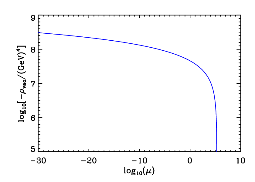
We are now in a position to conclude the first part of this review. The considerations of the previous sections lead to the following expression for the vacuum energy [51]
| (515) |
where indicates the contribution coming from the bared cosmological constant and where the dots means that other phase transition could contribute. Let us now evaluate the first term more precisely for the standard model of particles physics [51]. In this case, one has one scalar field, the Higgs boson with , GeV, the six quarks (fermions) for which and , , , , and , the leptons (fermions) with and , , , the neutrinos (fermions) the mass of which is so small that we can ignore them and, finally, the gauge bosons (massive vector fields), , and , . Of course, we also have the photon but since , as already mentioned before, it does not contribute to the vacuum energy. The only piece missing in order to calculate in Eq. (515) is the renormalization scale . It was argued in Ref. [51] that, because we use the photons coming from the supernovae to determine the cosmological constant and because these photons couple to the metric the expansion rate of which is characterized by the Hubble constant, one should take with and with the energy of the photons corresponding to the wavelength . This leads to and implies that Eq. (515) reads
| (516) |
If one does not want to estimate , one can simply plot as a function of as done in Fig. 5. Clearly, regardless of the precise value of , we are very far from always mentioned in the literature.
At this stage, Eq. (516) can be seen as the “prediction” of the standard model for the vacuum energy. At first sight, the calculation is straightforward and, in order to obtain the number in Eq. (516), we have used techniques of regularization that are known to work in similar contexts (i.e. when one computes a cross-section in particle physics) and to lead to a very good agreement with experiments. Therefore, we now turn to the question of what is known experimentally about the vacuum energy.
X Measuring the Cosmological Constant in Cosmology
Having discussed how the vacuum energy can be calculated, we now address the question of how it is determined and/or constrained experimentally/observationally. Here, we should distinguish the case of cosmology, treated in this section, and the other experiments, treated in the following sections. The difference is that, in cosmology, one claims a detection of while, as we will see, the other experiments can only put an upper limit on its value. Moreover, in cosmology, there are in fact many different and independent observables that can be used to measure the cosmological constant [23, 24, 79, 80, 81, 82]. All these techniques are reviewed in other articles [40, 41] and, therefore, it is not our purpose here to discuss this question in details. However, for completeness and also because this has some impact on the theoretical status of the cosmological constant problem, we now discuss how can be determined. We will do so from a theoretical perspective leaving, as mentioned before, the technical aspects to other articles [40, 41].
X.1 The Accelerating Universe
As is well-known, the claim that vacuum energy has been measured (and not only constrained) was first established from the discovery that the expansion of the universe is accelerated (although one can find many claims about the value of the cosmological constant in the history of cosmology) [23, 24]. Since the above mentioned claim has clearly very important consequences for physics, one needs to be very precise at this stage and this is why, in what follows, we will review the exact origin of this result.
In order to construct a cosmological model we apply general relativity to the Universe as a whole [83]. The cosmological principle implies that the Universe is, on large scales, homogeneous and isotropic. As a consequence, the metric is given by the following expression
| (517) |
where is the metric of the three-dimensional space-like sections and where is the scale factor. The expansion is characterized by the Hubble parameter, where a dot means a derivative with respect to cosmic time. In the standard model of cosmology, matter is assumed to be a collection of perfect fluids (at least in the simplest version) and, as a consequence, its stress-energy tensor is given by the following expression
| (518) |
where is the (total) energy density and the (total) pressure. These two quantities are related by the equation of state
| (519) |
[in general, there is an equation of state per fluid considered i.e. ]. The vector is the four velocity and satisfies the relation . In terms of cosmic time this means that . The fact that the stress-energy tensor is conserved, , amounts to
| (520) |
This expression is obtained when one takes . The case does not lead to an interesting equation for the background. Moreover, if we assume that the fluids are separately conserved, then the above relation is in fact true for each fluid, i.e. .
We are now in a position to write down the Einstein equations (10) for the Universe. We arrive at the following non-linear, second order, differential equations
| (521) | |||||
| (522) |
From the previous formulas, as already signaled in Eq. (11), we see that we can also define by and by . In this case, the cosmological constant is described as fluid with a constant energy density and pressure and with an equation of state , i.e.
| (523) |
This is of course consistent with Eq. (5). It is worth noticing that the vacuum energy is described by a fluid with a negative effective pressure.
Combining the two Einstein equations, one gets an equation which permits to calculate the acceleration of the scale factor
| (524) |
Let us notice that, in order to obtain the above formula, we have not assumed anything about the curvature . This equation is especially interesting because it gives the condition leading to an accelerated expansion, namely
| (525) |
Since the energy density of matter must be positive, we see that the above condition requires a negative pressure, i.e. some exotic form of matter. But, this is of course exactly what happens when the vacuum energy is the dominant fluid in the universe. Then, Eq. (524) can be written as which is positive for a positive effective cosmological constant. Therefore, in the framework of the standard model described before, the discovery that means that a fluid with a negative pressure is driving the expansion.
X.2 The Hubble Diagram
In this section, we explain how the measurement of the Hubble diagram can be used to infer the value of the cosmological constant.
Let us first consider a source in flat space-time whose absolute luminosity is given by (energy emitted per unit of time). This quantity can be written as
| (526) |
where is the number of photons emitted during the time interval . Suppose that we observe the source from a distance using a telescope, the surface of the mirror being . The number of photons received is given by
| (527) |
On the other hand, the flux of photons (or apparent luminosity i.e. energy per unit of time and surface) through the telescope is, by definition,
| (528) |
from which we deduce that
| (529) |
We have just recovered the well-known fact that the apparent luminosity of a source decreases as the inverse squared of the distance. On the other hand, we can use this relation as an operational definition of the distance, namely .
The previous considerations can be used as a definition of distance in cosmology. For this purpose, let us now consider the same situation but in a curved space-time with the following metric [a form more explicit than the one given in Eq. (517)]
| (530) |
We assume that the source is located at the co-moving coordinate while the observer is located at the origin of the coordinates. In order to reproduce the above flat space-time calculation in this new situation, we first need to calculate the surface of the sphere const., const. surrounding the source. The surface is just given by the integral of the covariant volume element, namely
| (531) |
This means that the number of photons received in the telescope can now be expressed as
| (532) |
But we have also to take into account the two following phenomena. Firstly, the energy of the photons has changed during the propagation from the source to the observer. If is the wavelength, we have , from which we deduce that , that is to say we have the redshift due to the expansion. Secondly, if the photons are emitted as a burst of duration , they will be received as burst of duration . We are now in a position where we can calculate the apparent luminosity. We obtain
| (533) |
where is the redshift of the source. Now if we use the operational definition of the luminosity distance (529), we find
| (534) |
We see from the last expression that the distance of a source depends on the behavior of the scale factor between the time of emission and the time of reception. On the contrary, if we measure the luminosity distance versus the redshift, we can learn about this behavior. Measuring the apparent luminosity is quite easy and, clearly, the difficulty lies in estimating the absolute luminosity of the source. It is also convenient to work in terms of the distance modulus, , since the data are often presented in this way. The quantity (or sometimes ) is the apparent bolometric magnitude. It is related to the apparent bolometric luminosity by
| (535) |
For instance the sun has an apparent bolometic magnitude of . On the other hand, the absolute bolometric magnitude is the apparent bolometric magnitude that the source would have at a distance of pc and is given by
| (536) |
For instance, the absolute bolometric magnitude of the sun is . As a consequence, using these two definitions, the distance modulus is defined by
| (537) |
such that is dimensionless and is of course nothing but the Hubble length (we have re-established the speed of light for convenience). From the above expression, one immediately deduces that
| (538) |
where is expressed in , in s and in Mpc.


In practice we only have access to over a limited range of redshifts. Therefore, one can derive a general expression by Taylor expanding the scale factor. For small redshifts, we have
| (539) |
where is the acceleration parameter. A positive acceleration parameter corresponds to a decelerating universe whether a negative one corresponds to an accelerating universe. Using the previous expression, the luminosity distance becomes
| (540) | |||||
| (541) |
As expected the result only depends on the time of flight . In order to obtain our final result, we must express this time of flight in terms of the redshift. The redshift of the source is defined by . Using the Taylor expansion of the scale factor, we end up with
| (542) |
which can be easily inverted to give the expression of the time of flight, namely
| (543) |
The last step is to replace the above expression into the Eq. (541). This gives
| (544) |
where we have taken into account that the time of reception is the present time (denoted with the subscript “0”). We see that the measurement of the luminosity distance versus the redshift allows us to determine the Hubble parameter today. If one goes sufficiently far in redshifts, one can determine whether the universe is accelerating or not via the accelerating parameter . It is worth noticing that this last conclusion is independent of the underlying gravity theory (provided this is a metric theory). The typical behavior of the luminosity distance and of the modulus is illustrated in Fig. 6 for a matter dominated universe. Let us also notice that the method that we have just presented for pedagogical reasons is of course not used in practice because we have now measured up to redshifts of for which the Taylor expansion is not valid (and, of course, in the real world the analysis is always more complicated that the simplified version discussed above). In this case, one must use an exact expression, that is to say one must compute the integral in Eq. (534) exactly.
If we now use general relativity (i.e. a specific theory for gravity), one can go further and relates the value of the acceleration parameter to the matter content of the Universe. The critical energy density , defined by , is used to evaluate the contribution of each species through the parameter where is the energy density of the species at present time. Then, the Friedman equation can be re-written as
| (545) |
and the acceleration parameter can be re-expressed according to
| (546) |
The universe contains pressure-less gas (cold dark matter and ordinary baryonic matter) for which but also radiation () and, finally, vacuum energy (). In this case, one obtains
| (547) |
Today, the contribution of radiation is negligible since we know from the measurement of the CMB that [81]. Therefore, the acceleration parameter is in fact given by . On the other, we also know that the universe is spatially flat which means that [81]. As a consequence, from the measurement of [23, 24], one can deduce the two quantities and . On finds that and . This is how one reaches the conclusion that our universe is accelerating and that vacuum energy dominates the present energy content. Remarkably, as announced at the beginning of this section, it is a detection and a measurement of . One finds
| (548) |
a number that should be compared with Eq. (516).
At this stage, several remarks are in order. Firstly, we notice the large mismatch between the theoretical expectation (516) and the above, observationally determined, number (548), something like orders of magnitude (but much less than the orders of magnitude often quoted in the literature). This is of course nothing but the cosmological constant problem although we will be more accurate with regards to its definition in the subsequent sections. Something is clearly wrong but, as will be discussed, it is difficult to identify where the mistake is. Secondly, it is clear that the above conclusion rests on many assumptions. For instance, we have assumed that the universe is homogeneous and isotropic [42] and that gravity is well described by general relativity. This means that, a priori, the cosmological constant problem is present in this context only. Thirdly, we have also implicitly assumed that the reason for the accelerated expansion is vacuum energy. This is clearly a natural idea since there is a term in our theory that must be present since it satisfies all the required properties (covariance, energy conservation) and that precisely leads to the observed phenomenon. A priori, nothing more can be asked to a new theoretical framework. But, given the mismatch discussed before, one can also doubt the identification of the source of the accelerated expansion with vacuum energy. As a matter of fact, it is possible to construct models where the universe accelerates because of some new source of matter (often named “dark energy”). This is for instance the case of quintessence and/or galileons [43] models where a scalar field is responsible for the acceleration. In this case, one can no longer claim that we have detected the vacuum energy and that its value is given by Eq. (548). However, this does not solve the cosmological constant problem because, even if the source of the acceleration is another fluid, we still have the constraint . Clearly, the number (516) does not satisfy this inequality which means that the problem is still present. In this sense, the constraint deduced from cosmology is very important: even if dark energy is not the cosmological constant, the observation that the energy density today is the critical energy density severely limits the value of . Fourthly, in principle, it is possible to check experimentally whether the reason for the accelerated expansion is vacuum energy or something else like quintessence [84, 85, 86, 87, 88, 89, 90, 91, 92, 93, 94, 95, 96, 97, 98, 99] (more recently, in Ref. [100], the current acceleration was also explained by a scalar field experiencing quantum fluctuations during inflation). Measuring the equation of state parameter is the clue since, if this is a constant equals to , then one can be sure that the source of the acceleration is the cosmological constant. Unfortunately, this measurement is difficult [101].
One more general grounds, it is clear that it would be better to have constraints, or even a measurement, of vacuum energy in an experimental context which is is not cosmology where, as reminded before, measurements are difficult and always subject to many biases and systematic errors. In the next sections, we explore whether this is possible.
XI Measuring the Cosmological Constant Elsewhere Than In Cosmology?
In the previous section, we have written the Einstein equation in an homogeneous and isotropic universe. Here, we investigate the influence of the cosmological term in a spherically symmetric situation. This will allow us to study how the presence of affects the motion of the planets in our solar system and how it modifies the energy levels of the Hydrogen atom.
XI.1 The Static and Spherically Symmetric Gravitational Field in Presence of a Cosmological Constant
Let us analyze the influence of the cosmological constant in a static and spherically symmetric situation [102]. This means that, in spherical coordinates, one can write the metric tensor as [102]
| (549) |
where and are two free functions. We seek solutions of the Einstein equations (10) with a vanishing stress energy tensor. It is easy to show that these equations can be expressed as
| (550) |
The next step is to calculate the components of the Ricci tensor for the metric tensor given by Eq. (549). Straightforward calculations lead to the following expressions
| (551) | |||||
| (552) | |||||
| (553) | |||||
| (554) |
the other components being zero. In the above equations, a prime denotes a derivative with respect to the radial coordinate .
We are now in a position where one can determine the solution of the field equations. If we take the combination [from the Einstein equations (550)], one obtains
| (555) |
which implies that , where is a constant. Using this expression, one can re-express as
| (556) |
and, as a consequence, the corresponding Einstein equation now reads
| (557) |
This equation can easily be integrated and one obtains
| (558) |
where is another integration constant. The constants and are fixed in such a way that, in absence of a cosmological constant, one recovers the standard Schwarschild solution. This amounts to take and , where is the mass of the central body and the Newton constant. This completes our calculation since the two functions and are now completely specified, namely
| (559) |
We can now compare this solution to the standard Schwarschild solution. The fact that the time-time component of the metric tensor is inversely proportional to the - component is still true but the radial dependence of the function is modified by the presence of a cosmological constant. In the Newtonian limit, we have , where is the Newtonian potential. In the present context, this implies that
| (560) |
Therefore, we obtain the usual gravitational potential corrected by a term proportional to the cosmological constant. This term looks like an inverted harmonic oscillator. This corresponds to a force felt by a test body of mass given by
| (561) |
where is a vector directed towards the central body of mass . The cosmological constant force is directed in the other direction and can therefore be viewed as a kind of “anti-gravity force”. We also notice that it is proportional to which means that its effect will be more important on large scales. This last property is the clue to understand why measuring the cosmological constant is more efficient on large scales (the best example being of course cosmology). This means that the modification of the planet orbits and/or the energy levels of the atoms will certainly be a small effect. On the other hand, we know that measurements in, say, atomic physics are extremely accurate and, a priori, there is the hope that this accuracy could compensate the smallness of the effect. Unfortunately, as we are now going to study, this will not be the case.
XI.2 Planets Orbits

Our goal in this section is to study how the planet orbits are modified by the presence of vacuum energy [103, 104, 105]. We will follow the treatment of Ref. [103]. We assume that the gravitational field created by the sun and the cosmological constant is given by Eqs. (549) and (559) with . The motion of a planet is represented by the motion of a test body in this background gravitational field. The corresponding geodesic equation can be written as
| (562) |
where is an affine parameter (not necessarily the proper time). Then, after having evaluated the Christoffel symbols for the metric (549), one can express these equations explicitly. One obtains
| (563) | |||||
| (564) | |||||
| (565) | |||||
| (566) |
Let us now solve these equations. Firstly, we can assume that the orbit stays in the plane. This automatically solves Eq. (565). Then, if we divide Eq. (563) by and Eq. (566) by , we obtain two new equations, namely
| (567) | |||||
| (568) |
The first equation can be used to define the affine parameter. We choose it such that it satisfies . Then, the second equation tells us that
| (569) |
where is a constant. Finally, Eq. (564) can be re-written as
| (570) |
If we multiply this last equation by , one arrives at
| (571) |
This means that the quantity inside the square brackets is a constant. Let us call this constant . Then, this gives an equation expressing how the radial coordinate varies with the angle ,
| (572) |
It is easy to express the constants and in terms of the aphelion and perihelion and , which are the two points on the orbit such that , see Fig. 7 (where the elements of the orbits are represented). This gives
| (573) | |||||
| (574) |
with defined by .
So far, we have been very general and we have never specified the function . From now on, we are going to use the explicit form of this function, see Eq. (559). Let us notice in particular that, in absence of a cosmological constant and in the limit where , the two above expressions reduce to
| (575) |
where (of course, not to be confused with the integration constant introduced in the previous sub-section). As is shown in the following footnote, these are exactly the relations obtained in the Newtonian case. More generally, Eq. (572) takes the form
| (576) | |||||
Performing the standard change of variable, and differentiating with respect to , we obtain 44 4 It is interesting to compare this result with the Newtonian analysis. In this case, the Lagrangian is given by (577) where a dot denotes a derivative with respect to time. Again we have chosen the orbit to be in the plane . This leads to the following equations of motion (578) (579) The second equation gives while the first one can be re-written as (580) The quantity between the parenthesis is a constant and we call it . Then, this equation can be re-expressed as (581) From this equation one can deduce an expression for and in terms of the aphelion and the perihelion. One gets (582) Introducing the variable and differentiating once more with respect to , one arrives at (583) This equation can easily be integrated. The solution reads (584) where and are two arbitrary constants. Clearly, one can always take . The above trajectory represents, as is well-known, an ellipse with eccentricity .
| (585) |
This is the differential equation that needs to be solved in order to find the trajectory of the planet. It should be compared with its Newtonian counterpart, see Eq. (583). One can check that, in this regime (without a cosmological constant), the two equations are indeed identical since according to Eq. (575), , and the term can be neglected. The relativistic term is responsible for the precession of the perihelion and the last term represents the correction due to the cosmological constant.
We now turn to the solution of Eq. (585). Let us first review how one calculates the precession of the perihelion without a cosmological constant [102]. The idea is to restart from Eq. (576). For , the polynomial on the right hand side can be written as
| (586) |
since we know it has to vanish at . The only quantity that remains to be determined in this expression is . Comparing the above relation with Eq. (576), we deduce that
| (587) |
Using the expressions derived before, it is easy to show that . As a consequence, one can write
| (588) | |||||
There are several methods to evaluate this integral. As a matter of fact, it can be integrated exactly in terms of Elliptic functions [48, 49]. But, being given that is a small quantity, it is better to expand the result in this parameter. This leads to easier calculations that are, moreover, more explicit. In addition, the method can be generalized to the case of a non-vanishing cosmological constant, which is of course our main goal. In fact, if we restart from Eq. (572) and use that , we see that the term in the squared bracket in Eq. (572) is a quadratic function of which vanishes at . This means that one necessarily has
| (589) |
Then, writing Eq. (572) in terms of rather than , one arrives at
| (590) |
Now, when , as is clear from Eq. (576), the term in the square bracket of Eq. (572) is no longer a quadratic function of even if the expansion of the function is used. However, this term still vanishes at and the integral will be dominated by the contributions coming from the vicinity of these points, see also Eq. (588). The idea is then to continue to work with Eq. (589) and to take into account the cosmological constant in the definition of [103]. This should provide a reasonable approximation of . Using Eqs. (573) and (574), one can write
| (591) | |||||
Then, if we differentiate both sides twice with respect to , this gives
| (592) | |||||
| (593) |
where is the semilatus rectum. In the above expression, we have used . So far, the method is completely general provided that . We now use the explicit form of . Expanding everything in and in , one obtains [103]
| (594) |
The final step consists in using the above expression in Eq. (590). One finds [103]
| (595) | |||||
where we have expanded and where we have used the fact that , the complex being exactly cancel by the coming from the fact that , which appears in a square root, is negative [its expansion starts with , see Eq. (594)]. As a consequence, we obtain
| (596) |
where the first term is the standard relativistic perihelion precession while [103]
| (597) |
is the contribution due to the cosmological constant. The above equation is the main result of this sub-section. It gives the perihelion precession due to the presence of vacuum energy. Let us notice that the scaling indicates that the precession is larger for planets that are far from the Sun. It is of course totally consistent with the fact that the effect of the cosmological constant is more important on large scales.
We now use the above result to constrain the amount of vacuum energy present in our universe. For this purpose, let us now calculate this perihelion shift for, say, Mercury (as mentioned before, the effect is larger for other planets but this does not modify the conclusions obtained below; estimates for Venus, Earth and Mars can be found in Ref.[105]). In this case, we have and . This implies that . We also have . Finally, it is interesting to calculate in terms of the vacuum energy density observed in cosmology, see Eq. (548). For the cosmological constant, this leads to the following number . This leads to the following expression
| (598) |
or, since Mercury completes revolutions each century and there are arc-seconds per radian,
| (599) |
which is, of course, completely unobservable. The reason for such a result has already been mentioned. The solar system has a characteristic scale (say a few astronomical units) which is too small for the cosmological constant to leave a sizable imprint. However, even if one cannot measure the vacuum energy density with this method, it can nevertheless be used to constrain its value. Indeed, the uncertainty in the precession of the perihelion of Mercury is about par century, which means that
| (600) |
implying that
| (601) |
Of course, this limit is not competitive with what one has obtained in cosmology. However, when compared to Eq. (516), it leads to an interesting piece of information which allows us to define what the cosmological constant problem is more accurately. Indeed, we see that there is a contradiction between the theoretical expectation (516) and the observations of the planet trajectories in our solar system. In other words, the predictions of Eq. (516), if true, would lead to orbits drastically different from what we observe. Therefore, even without the cosmological observations and only from the motion of the planets in the solar system, one sees that our calculation of vacuum energy must be incorrect. Put it differently, it would be incorrect to say that the cosmological constant problem originates only from the recent astrophysical observations. In some sense, the problem is much worse. Only by observing the planets in the solar system, a class of observations which seems to be much more straightforward than the cosmological observations, we know that our regularization method of the vacuum energy must be flawed.
XI.3 Modifications of the Atomic Levels
We have just seen that observing the motion of planets in our solar system can tell us something about the value of the vacuum energy. A priori, another possibility to observe the influence of the cosmological constant is through the modification of the atomic energy levels that its presence would cause. In this section, we investigate this question in the case of the Hydrogen atom since this is technically simple [106, 107, 108, 109, 110, 111]. We will follow the treatment of Ref. [106]. In particular, since the problem is still spherically symmetric, one can use the metric tensor (549) obtained before.
The motion of an electron around the nucleus, living in a static and spherically symmetric manifold, is described by the following Dirac equation
| (602) |
where is a Dirac spinor, see Sec. VII.1 and the mass of the electron. In the above equation, are the Dirac matrices satisfying the relation
| (603) |
Let us notice that we have already presented this formula, see Eq. (332). Here, we slightly change the notation and now denote the Dirac matrices in curved space-time by (notice that we have also included a factor in the definition of ). The matrices are related to the Dirac matrices in flat space-time, , by , where are the vierbein fields such that . The symbol denotes the covariant derivative acting on the spinor, namely
| (604) |
where the spinorial connection can be expressed as
| (605) |
with and is the vector field describing the electromagnetic field acting on the electron ( is the charge). The Dirac equation can also be re-written as
| (606) |
where the effective Hamiltonian is given by
| (607) | |||||
In this case, the Dirac equation looks like an effective Schrödinger equation.
It is clear that the typical dimension of an atom is very small in comparison to the typical curvature scale of the manifold. Therefore, as was done for the calculation of the Green function in Sec. VIII, one can perform a local analysis. For this purpose, we now use the Fermi normal coordinates [78]. In these coordinates, the metric tensor takes the form
| (608) | |||||
| (609) | |||||
| (610) |
where the dots indicate higher order terms. This implies that the veirbein fields can be expressed as
| (611) | |||||
| (612) |
and the Christoffel symbols can be written as
| (613) | |||||
| (614) | |||||
| (615) | |||||
| (616) |
Using the above results, this finally leads to the following expression for the spinorial connection [106]
| (617) | |||||
| (618) | |||||
The above formulas will allow us to calculate the effective Hamiltonian (607) explicitly. But before reaching this stage, we must also determine vector field . The Lagrangian of the corresponding gauge field is given by, see also Eq. (369)
| (619) |
from which we deduce that the equations of motion read
| (620) |
At first order in the curvature, these equations can be expressed as [106]
| (621) | |||
| (622) |
For a one electron atom with a nucleus of charge , one can take
| (623) |
In what follows, we determine the vector perturbatively in the curvature. At zeroth order, in flat space-time, the equation for the time component reduces to
| (624) |
whose solution is of course
| (625) |
Then, we write , where is first order in the curvature. By inserting this expression into the full equation (621) and using the zeroth order solution (625), one arrives at [106]
| (626) |
The solution of the above equation reads [106]
| (627) | |||||
In the same manner, one can determine the space component. Obviously, at zeroth order, one has . The first order perturbation obeys the equation [106]
| (628) |
whose solution can be written as [106]
| (629) |
This completes our calculation of the electromagnetic field.
Having determined the vierbeins fields (i.e. the quantities describing the gravitational force) and the gauge field (i.e. the quantity describing the electromagnetic force), we are now in a position where we can calculate the Hamiltonian (607). In order to make contact with the usual treatment of the Hydrogen atom, it is more convenient to introduce the standard Dirac matrices and related to the flat space-time Dirac matrices by
| (630) |
As is well-known, they satisfy
| (631) | |||||
| (632) |
Then, we use the expressions of the spinorial connections (617), of the gauge field (625), (629) and of the Dirac matrices in the equation (607) of the Hamiltonian. This leads to the following expression
| (633) | |||||
In this expression we have defined and we have taken . The three first terms are the usual Dirac Hamiltonian. The other terms represent the correction due to space-time curvature. Since the above expression is quite complicated, it is interesting to estimate the order of magnitude of each term. The curvature is given by where is a typical distance. Each is typically of the order of the Bohr radius, i.e. . As a consequence, is of order . This also means that the typical velocity is given by . Of course the matrices and are dimensionless but, in the non relativistic limit must reduce to which implies that . In the following we consider that where is the fine structure constant is a small number. Then, the dominant term in the above expression is the last one, which means that the Hamiltonian can be approximated as
| (634) | |||||
where we have used . If we use the following representation for the Dirac matrices
| (635) |
and write the Dirac spinor as
| (636) |
then the Dirac equation reduces to two equations that can be expressed as
| (637) | |||||
| (638) |
From the second relation we can express in terms of and then we can insert this expression into the first equation. This leads to
| (639) |
or, using and expanding the denominator of the first term in the above equation
| (640) |
But, if we now perform an additional expansion assuming non-relativistic velocities for the electron (which, in practice, is a good approximation), one arrives at the following expression for the term
| (641) |
As a consequence, we conclude that the non relativistic limit is given by
| (642) |
where the non-relativistic Hamiltonian can be written as [106]
| (643) | |||||
This is our final result. Endowed with this equation, one can calculate, by means of perturbations theory, the modification of the ground state due to the presence of a cosmological constant. This leads to (the arguments of indicates the value of the quantum numbers and )
| (644) | |||||
| (645) | |||||
| (646) |
The ground state wave function is given by (at this order of perturbations theory, there is no need to take into account the modification on the wave-function; one can use the standard one)
| (647) |
where we recall that is the Bohr radius. This implies that
| (648) |
The vacuum Einstein equations are, see Eq. (550), and, therefore, at first order in the cosmological constant one (here, of course, we only compute the corrections due to the cosmological constant and not those originating from the Earth gravitational field). This means that
| (649) |
where we have re-established the speed of light for convenience. In fact, this result could have been anticipated from the Newtonian approach. Indeed, we have seen that the Newtonian potential, in presence of a cosmological constant, is given by , see Eqs. (560) and (561). Using the perturbation theory with this potential exactly leads Eq. (649). Let us now evaluate the correction. Using that the reduced mass of the atom is essentially the electron mass, and that the Bohr radius is , one obtains
| (650) |
a quantity completely unobservable, probably for ever. For comparison the Lamb shift is of the order . At this stage this does not come as a surprise. As discussed in the case of planet orbits, the size of the system is so small that the influence of the cosmological constant is negligible. However, requiring that the shift due to the cosmological constant be smaller than the Lamb shift leads to
| (651) |
This result is less good than the one obtained from planet motion by about orders of magnitude. Moreover, the theoretical expectation (516) satisfies this inequality. Let us notice in passing that the result based on the wrong regularization scheme, does not satisfy the previous bound.
We now have a clearer view of what the cosmological constant problem is. On one hand, one can calculate the vacuum energy density by means of, apparently, well known techniques of regularization. These techniques usually lead very robust results, fully consistent with the observations. For instance, the radiative corrections to the calculation of cross-sections have proven in very good agreement with various high energy physics experiments. One the other hand, various observational results (and not only in cosmology) indicate that the previous calculation is not correct. The theoretical expectation value for the vacuum energy density is so large that it should have already be seen by many experiences. Moreover, in cosmology, under a certain number of hypothesis, one even measures which is found to be many orders of magnitude smaller than the number derived from the theory. Since, as mentioned before, the theoretical framework seems to be robust (let us recall again that it involves calculations that can be found in the first pages of any textbook on quantum field theory) and since the observations seem to be convincing, we are facing a genuine mystery. However, before accepting this conclusion, it is worth checking that no loophole is present in the previous reasoning. This will be the goal of the next sections. A first question that can be asked is whether the zero-point fluctuations that are at the origin of the problem are a real physical phenomenon or just an artifact of the formalism of quantum field theory. We turn to this issue in the next section.
XII Do the Vacuum Fluctuations Really Exist?
We have seen in the previous sections that the zero-point fluctuations manifest themselves as the vacuum energy. Since this leads to conclusions that seem to be in contradiction with observations, it is legitimate to ask whether these fluctuations really exist in Nature. In particular, we want to investigate whether the zero-point fluctuations could manifest themselves in other physical phenomena. The answer to this question is usually positive and one experiment which is considered as a proof that the vacuum fluctuations are real is the measurement of the Lamb shift [112, 18]. In the next sub-section, we discuss this phenomenon.
XII.1 The Lamb Shift
Let us consider the “motion” of an electron in an atom. Its “location” is described by the vector . The vector is going to fluctuate because of the interaction between the electron and the zero-point fluctuations of the electromagnetic field. This interaction will slightly modify the position of the atomic levels leading to the Lamb shift. Let us study in details how this effect can be derived. Let be the Coulomb potential which determines the properties of the atom. At the point , the potential can be Taylor expanded according to
| (652) |
Then, if we time average the previous expression, one obtains
| (653) |
and, because the problem is spherically symmetric, we have and . The first term in Eq. (653) is the unperturbed Coulomb potential and the last one (since the second one vanishes) can be viewed as a small perturbation of the Hamiltonian, namely
| (654) |
In an atom with atomic number , the Coulomb potential is given by
| (655) |
where is the fine structure constant. This means that .
Let now us assume that the atom is placed in the quantum state . As we have already discussed in Sec. XI.3, at first order, the time-independent perturbations theory tells us that the correction to the energy of the level is given by [57]
| (656) |
Using Eq. (654), one obtains the following expression for the energy displacement
| (657) |
where is the wave-function in the corresponding quantum state. Since the wave-function at the origin can be expressed as [57]
| (658) |
where is the electron mass () one finally arrives at [18]
| (659) |
Therefore, we have reduced the problem to the calculation of the quantity . In order to evaluate this quantity, we must now evaluate the displacement of the electron. The electron “moves” under the influence of the electric field within the atom and, as a consequence, obeys the following equation
| (660) |
where is the electric field (or, rather, its vacuum fluctuating component). Using the usual expansion of the vector potential in terms of creation and annihilation operators, see Eq. (395), one can write
In the same manner, one has to Fourier expand which is considered as an operator in this context. One obtains
| (662) | |||||
The Fourier amplitude of the displacement operator can be calculated from the equation of motion (660). This leads to the following expression
| (663) |
From this expression, one can now evaluate the quantity . One finds
| (665) | |||||
where we have used . Therefore, inserting the above formula into Eq. (659), one obtains the following equation for the energy shift [18]
| (666) |
This equation is the main result of this section. It gives the energy levels displacement due to the presence of the electromagnetic zero-point fluctuations.
As usual this expression is divergent and needs to be regularized. In a simplified treatment, one simply assumes, see Ref. [18], that the wavelengths in the above sum must be larger than the Compton wavelength of the electron, which implies and that , where is the Bohr radius. In this case, the previous results reduces to
| (667) |
Let us now evaluate this quantity for the Hydrogen atom. Clearly, there is no effect for . But for and , one has
| (668) |
where we have used with .
This shift has been experimentally observed and is usually taken as a proof that the zero point fluctuations are real since they lead to an observed physical phenomenon. Based on this result, it now seems difficult to argue that the zero-point fluctuations are just an artifact of the formalism of quantum field theory. Moreover, there exists another experiment, the Casimir effect, where the effects of the vacuum fluctuations can be observed. In the next section, we investigate this case.
XII.2 The Casimir Effect

In this section, we study the Casimir effect [113, 114, 115, 116, 117, 118, 119]. Since its discovery, this effect has been studied in great details and it is clear that, here, one cannot review all the literature. We will give a description of this phenomenon in a simplified context only and will refer to Refs. [113, 114, 115] for readers interested in learning more about this interesting subject.
XII.2.1 The Casimir Force
Let us consider an experimental situation where we have two conducting plates in the plane separated by a distance long the direction, see Fig. 8. For simplicity, instead of considering the electromagnetic field in the cavity (which is the case in the real world, especially when measurements are performed), we will just treat the case of a real massive scalar field . This field obeys the Klein-Gordon equation already studied and solved before, see Eq. (60), except that now the boundary conditions are modified by the presence of the two plates. Let us write . Then, inserting this anzatz into the Klein-Gordon equation, one obtains
| (669) |
where is the mass of the scalar particle. Clearly, one can separate the variables and, as a consequence, the above equation can be split into four differential equations, namely
| (670) | |||||
| (671) | |||||
| (672) | |||||
| (673) |
where the constants , , and are related by
| (674) |
The solution in the and direction can be expressed in terms of standard plane waves, and . The quantities and are just integration constants. Of particular interest is of course the solution along the -axis. It can also be written as
| (675) |
where and are two integration constants. But the difference with the case of a free field is that the boundary conditions “feel” the presence of the two plates. These boundary conditions are given by and . The first one implies that while the second one gives
| (676) |
or, equivalently,
| (677) |
where is an integer. Finally, the equation for the function can also be easily solved and the solution reads
| (678) |
where . Therefore, upon using Eq. (674), the frequency takes the form
| (679) |
In this expression, and take continuous values.
Based on the previous considerations, one can now write the field operator as an expansion in terms of creation and annihilation operators. But this expansion encodes the fact that, along the -axis, the wave-number is discrete. Concretely, we have
| (680) |
The operators and obey the usual commutation relations for bosons. It is interesting to check that the above expansion is indeed consistent with the commutation relations between the field and its conjugate momentum. For this purpose, let us compute the following quantity
| (681) | |||||
Using the fact that (as can be checked directly) and one arrives at
| (682) |
In the same manner, one can also evaluate the following integral involving the conjugate momentum (a dot means a derivative with respect to time)
| (683) |
From the two above expression, one can deduce a formula expressing the creation and the annihilation operators in terms of the field operator and its conjugate momentum. One obtains
We are now in a position where we can compute the commutator of a creation and an annihilation operators. It can be written as
| (684) | |||||
Then, we make use of the canonical relation in the previous formula. This leads to the following complicated expression
| (685) | |||||
| (686) |
We have thus reached our goal, namely we have shown that the canonical commutation relation between the field and its conjugate momentum implies the usual commutation relation between the creation and the annihilation operator.
We are now in a position where we can evaluate the energy density of the field in the Casimir cavity. It is of course given by the same expression as in the free case, see Eq. (67). This means that one should first calculate the three terms that participate in the expression of , see Eqs. (64), (65) and (66). Let us start with . Using the Fourier expansion of the field and the commutation relations established above, one obtains
| (687) | |||||
and, if we integrate over the cavity volume
| (688) |
where is the area of the plates (of course, the two parallel plates have the same surface). In the same manner, one finds
| (689) |
Finally, the last relevant term reads
| (690) |
Putting everything together and using the definition (67), the expression of the energy of the field within the empty cavity takes the form
| (691) | |||||
| (692) | |||||
Of course, this expression has exactly the expected form. Roughly speaking it can be written as “”, see Eq. (679), the only difference being that, along the -axis, the sum takes into account the fact that the momentum is discrete. Another common point with our previous considerations is that the above number is actually divergent and must be regularized. In the following, we assume for simplicity and use dimensional regularization. Therefore, the expression of the energy can now be written as
| (694) | |||||
where is the “dimension” of the plates (i.e. in the real world) and denotes the wave-vector living in the sub-manifold defined by the plates. Then using the change of variables and the following definition [48, 49] of the Euler’s integral of first kind
| (696) |
the energy can be re-expressed as
| (697) |
The above formula can be expressed in term of the Riemann zeta function defined by the following expression
| (698) |
Moreover, upon using the two following equations
| (699) | |||
one can re-write the energy as
| (701) |
The Casimir force arises because of a shift in the vacuum energy when the plates are present compared to the situation where they are absent. So the relevant quantity is in fact where is the above quantity in the limit . As a consequence, for , one arrives at
| (702) |
where we have used . Therefore, the corresponding force is given by [113, 114, 115, 116]
| (703) |
which is one half the result obtained in the case of the electromagnetic field since we have only one state of polarization instead of two. We notice that the force is attractive (this could change in the case of more complicated geometries).
It is also interesting to check that the final result is independent from the regularization scheme used to obtain it. In order to test this idea in the simplest situation (i.e. where the calculations are easy), let us consider again the energy of a Casimir cavity but, this time, with . In this case, our zeta-function regularized result reads
| (704) |
since and . One the other hand, we can return to the expression of in Eq. (697). In the case , the energy density reads
| (705) |
In order to regularize this divergent quantity, we now proceed differently and introduce an exponential cut-off such that (previously, we argued that introducing a cut-off was not a good method because this breaks Lorentz invariance. Here, of course, this objection is no longer valid as the presence of the two plates along the -axis obviously breaks translation invariance; as a consequence working with a cut-off seems legitimate in the present context)
| (706) |
The sum is easy to perform and one obtains
| (707) | |||||
| (708) |
Now, the regularized Casimir energy is the shift energy in the vacuum after having sent the cut-off to zero; in other words
| (709) | |||||
| (710) |
that is to say exactly the same expression obtained with another regularization scheme. It is reassuring to notice that the final result is independent of the regularization method used.
XII.2.2 The Casimir Stress-Energy Tensor
In this section, we aim at calculating the stress energy tensor of a scalar field in a Casimir cavity [119, 113, 114, 115, 116]. Our goal is of course to compare this tensor with the vacuum stress-energy tensor . Here, we use a method based on the calculations of the Green function. This is yet another method of calculation of the Casimir effect, different from the two ones exposed before and, therefore, it will be interesting to compare this approach with the treatments used previously.
Let us start with the calculation of the Green function. It obeys the following equation
| (711) |
It is interesting to compare the above formula with Eq. (482). It is clear that this is the same equation but with (flat space-time) and (mass-less field). In order to solve this equation, it is convenient to Fourier transform in frequency and transverse momentum. Explicitly, one writes
| (712) | |||||
Inserting this expression into the Green equation (711), one obtains
| (713) |
where we have defined
| (714) |
Our goal is now to determine explicitly the Green function. Let us start with the solution within the plates, i.e. . When , the solution can be written
| (715) |
where and are two unknown function of . We must now take into account the boundary conditions. If , the condition implies that and therefore (for ). On the other hand, if , the condition means that
| (716) |
We have two unknown quantities and, therefore, we need two equations. One is provided by writing the continuity of the Green function when . The other is obtained by integrating Eq. (713) from to . This gives
| (717) |
which leads to
| (718) |
Therefore, taking the limit , the solutions of these two equations (i.e. the one expressing the continuity of the Green function and the one we have just derived) read
| (719) | |||||
| (720) |
As a consequence, the Green function between the plates can be expressed as [116]
| (721) |
The same method can be used to determine the Green function outside the cavity. Let us apply it for and larger than , i.e. on the right hand side of the cavity. In this case, it is more convenient to re-write the general solution (715) as
| (722) |
When , we require only one branch to be present which amounts to take . For , the boundary condition is still . Then, straightforward manipulations lead to [116]
| (723) |
which completes our determination of the Green function. The calculation of the Green function outside the cavity, but on the left hand side, proceeds exactly in the same way. The corresponding expression is obtained from the one above with , reflecting the fact that the boundary condition is now .
Endowed with the Green function of the problem, one can now turn to our main goal, namely the calculation of the stress-energy tensor. We have already seen that, see also Eq. (101),
| (724) |
But we know that the component of the stress energy tensor can be expressed as, see Eq. (7),
| (725) |
Therefore, if we apply the following operator to the Green function in Eq. (724)
| (726) |
where means a derivative with respect to , to and, then, take the space-time points to be the same , one should obtain an expression for . Using Eqs. (712) and (714), the result reads
| (727) | |||||
Then, we use the expression of the Green function inside the plates (721) and one arrives at
| (728) | |||||
| (729) |
In order to evaluate this integral, we perform the two Wick rotations and . This leads to
| (730) |
Then, we introduce polar coordinates in the plane , i.e. and . This gives
| (731) | |||||
| (732) |
Finally, writing that
| (733) |
the expression of can be re-expressed as
| (734) | |||||
The last step of the calculation consists in evaluating the last term [we call it in what follows; not to be confused with the Green function] of the above equation. One has
| (736) | |||||
where we have expanded the denominator in a geometric series. The two above integrals can be expressed in terms of the Hurwitz zeta function defined by [48, 49]
| (737) |
and this leads to
| (738) |
If we use the fact that , one arrives at our final expression for the time-time component of the stress energy tensor, namely
| (739) |
Of course we notice that the first term in the above equation is similar to Eq. (702).
Let us now evaluate outside the cavity. The calculation proceeds along the same lines but we now need to use the Green function given by Eq. (723). Straightforward manipulations lead to
| (740) |
We obtain the same structure as inside the cavity, namely a divergent term and a surface divergence term, i.e. a term which is divergent only on the plate. As explained in Ref. [116], this type of terms can be removed by restoring conformal invariance.
Let us now calculate the quantity inside the cavity. Clearly, following the previous considerations, it can be written as
| (741) | |||||
Following exactly the same procedure as before, we arrive at
| (742) |
Let us now calculate outside the plates. As we did for the time time component, we must now use the Green function (723). This gives
| (743) | |||||
| (744) |
Of course, this quantity is divergent.
Finally, in order to complete the determination of the stress-energy tensor, one must calculate . It can be expressed as
| (746) | |||||
A first step consists in dealing with the terms proportional to . In fact these terms are of the form , where represents the other terms in the integral which are function of only. Therefore, one can evaluate them by going to polar coordinates in the plane . This leads to an expression of the form , which shows that the corresponding contribution vanishes. Then, following the same steps as before, one reduces the above expression to
| (747) | |||||
where we have used that . Of course, as already mentioned, this also shows that . All the other components being zero, this completes our calculation of the stress energy in the cavity. Only the calculations of outside the plates remains to be done and we now turn to this question. Considering again Eq. (746), we have
| (748) | |||||
We are now in a position where we can write the full stress energy tensor. Inside the cavity, it takes the form
| (749) | |||||
where we have defined the two quantities and by
| (750) |
Outside the cavity (more precisely on the right hand side), the results derived above imply that
| (751) |
As discussed in Ref. [116], the terms proportional to and are surface divergent terms. They can be removed in the case where conformal invariance is re-established and, for that reason, are not present in electromagnetism, i.e. when one considers an electric field inside the cavity rather than a scalar field. In this case, we see that the difference between the stress-energy tensors inside and outside the cavity reads
| (752) |
which is a finite result. The infinite part has been removed by subtraction. Finally, the stress energy tensor can be written in a covariant form, namely [119]
| (753) |
where in the unit vector in the direction.
At this point, several comments are in order. Firstly, we notice in Eqs. (752) and (753) that the energy density (i.e. the time-time component) is similar to the expressions already derived in Sec. XII.2.1 by other methods. This confirms that this calculation is independent of the regularization scheme used to obtain the result. Secondly, it is clear that the stress-energy tensor (753) is not similar to the cosmological constant stress-energy tensor . This illustrates the difference between the Casimir case and the cosmological constant case. In the latter case, one measures the absolute value of the vacuum energy while, in the former case, one is only sensitive to the difference of vacuum energy from one side of the plates to the other.
Thirdly, the Casimir Force has been observed in the laboratory and this is usually taken as another evidence in favor of the existence of the zero-point fluctuations. After all, since we observe the Casimir force and since this force is due to a change in the structure of the vacuum that is perturbed by the presence of the plates, the fact is that the vacuum must exist as a real physical phenomenon and is not an artifact of the quantum field theory formalism. In addition, this also validates the methods of regularization used to calculate . In the context of the Casimir effect, these methods seem to work very well and to lead to predictions that are in agreement with the experiments. Therefore, why would the very same techniques, used in a similar context, fail to regularize the cosmological constant?
Fourthly, the claim that the calculation and the observation of the Casimir force are evidences in favor of the reality of vacuum fluctuations has been challenged in Refs. [120, 121]. It is indeed possible to derive the expression of the Casimir force without referring at all to zero point fluctuations, by means of the “source theory” approach to quantum field theory. However, to our knowledge, there is no attempt to do the same for the Lamb shift (but this would certainly be an interesting exercise). Therefore, it seems that zero-points fluctuations are nevertheless necessary to quantum field theory even if the above remark should lead us to tone down the claim that they have been seen in the laboratory. Let us also notice that, very recently, another situation where the vacuum fluctuations can lead to an observable effect has been studied in Ref. [122]. This article investigates whether the quantum zero point fluctuations could cause the rotation of a small nano device. This “rotational vacuum effect” has in fact a similar origin than the Casimir effect.
Finally, it should be clear that, if the Lamb shift and the Casimir effect seem to indicate that the vacuum fluctuations are real, they do not say anything with regards to their gravitational properties. In other words, they do not say how the vacuum fluctuations weigh (it is worth noticing here that the gravitational properties of a Casimir cavity have been studied in Refs. [123, 124, 125, 126, 127, 128, 129]). It is clear that there exists the possibility that the zero-point fluctuations do exist but have non-standard gravitational properties, i.e. that they abnormally weigh. It is therefore interesting to investigate if there is an experiment which measures whether this is true or not. In the next section, we turn to this question.
XIII Do the Quantum Fluctuations Gravitate?

In this section, we study the gravitational property of the Lamb shift [12, 130]. We will follow the treatment of Ref. [130]. In Sec. XII.1, we showed that the interaction of the electron with the “vacuum electric field” inside the atom leads to a shift of the atomic levels. In some sense, this means that the zero-point fluctuations affect the mass (energy) of the atom. Therefore, by studying how the atom falls down, one can put constraints on the gravitational properties of the vacuum fluctuations. This is the idea that we pursue in this section. However, since the corresponding effect is small for an atom and is larger for a nucleus (of course, the Lamb shift also exists in this case), it is better to study the latter case. For this reason, we start with recalling some basics facts about nuclear models.
The main idea is that the interaction between a given nucleon and the other nucleons can be mimicked by a Woods-Saxon potential given by
| (754) |
where describes how abrupt the potential is while is the radius of the nucleus. As is well-known one can take where . The quantity represents the depth of the potential and can be taken to be . In fact, in order to have a reasonable model, one must add to the Woods-Saxon potential a spin orbit interaction term which can be expressed as
| (755) |
where is the angular momentum of the nucleon and its spin. With a good approximation, one can write . Then, the Hamiltonian of the nucleus can be written as
| (756) |
The total wave-function can be taken as the product of the individual wave functions (in fact, more precisely, one should consider a Slater determinant in order to take into account the fact that the total wave function must be anti-symmetrized), that is to say
| (757) |
Each individual wave-function can be obtained from a Schrödinger equation given by (for the moment, one ignores the spin orbit term since it can be treated as a perturbation)
| (758) |
where is the reduced mass,
| (759) |
or , being the proton mass. Unfortunately, the Schrödinger equation cannot be solved analytically for the Woods-Saxon potential and, therefore, we are forced to make approximations. The simplest one is just to describe the Woods-Saxon potential with a parabola, i.e.
| (760) |
with . In this case, the question becomes solvable. We can use the spherical symmetry of the problem and write the wave function as
| (761) |
where is a spherical harmonics [48, 49]. The radial function is controlled by the equation
| (762) |
which can be solved in terms of Laguerre polynomials [48, 49]. Explicitly, one has
| (763) |
where is a normalization constant to be determined. In the above expression, one has and . The energy levels are given by the expression
| (764) |
The factor originates from the fact that we have a three-dimensional harmonic oscillator. The quantum numbers have been chosen so that the ground state is , which allows the spectroscopic notation “”, see Fig. 9.
The only thing which remains to be done is to determine the constant . Obviously, this is done by normalizing the wave-function, i.e.
| (765) |
Using the solution obtained above and performing the change of variable , the previous condition reduces to
| (766) |
Then, using Eq. (7.414.3) of Ref. [49], one obtains
| (767) |
We are now in a position where we can compute the value of the wave-function at for . This gives
| (768) |
Using the fact that , one obtains
| (769) |
This completes the first part of the calculation.
We have established on very general grounds that the shift in energy due to the interaction of a charged particle (in Sec. XII.1, the electron in the atom, here the proton in the nucleus) is given by Eq. (657). The means value of the square of the displacement has been calculated in Eq. (665). Applying these formulas to the case of the protons in the nucleus, one obtains [130]
| (770) |
As usual, this infinite integral must be regularized and usually leads to logarithmic corrections, see for instance Eq. (667). We will ignore this factor in what follows since this does not affect too much the final result. As explained in Ref. [130], the sum over “” runs only over -wave since this is the only way to get . Moreover, still following Ref. [130], it is reasonable to approximate the field experienced by a proton by a field produced by the other protons in inner shells. This is why represents the total number of protons present in shells inner than the proton “” under consideration.
Our goal is now to test how the vacuum fluctuations weigh. For this purpose, we write the gravitational mass of a given nucleus as [130]
| (771) |
where is the inertial mass. The parameter is a priori a free parameter which controls to which extent the weak equivalence principle would be violated. If , there is no violation of the universality of free fall. A convenient measure of potential violations of the weak equivalence principle is given by the Eötvös ratio
| (772) |
for two bodies and . Using the previous calculations, this ratio can be expressed as
| (773) | |||||
where we have used , a relation valid since we work at first order in the parameter . Then, we use the fact that
| (774) |
to express the Eötvös ratio as [130]
| (775) | |||||
Let us evaluate this number for aluminum (, ) and Platinum (, ). In the case of aluminum, since we only have protons, the only -shell protons are on the level (in fact, we have two protons in , four protons in , two protons in and five protons in , see Fig. 9). As a consequence, there is no inner protons for those protons (since, obviously, there is no inner level than the ground state ) and the corresponding contribution in the Eötvös ratio vanishes. In the case of Platinum, all the levels are filled up until the level which contains height protons, see Fig. 9. Therefore, we have two protons on , two protons on and two on , see again Fig. 9. This means that the protons see four inner protons and the protons see two inner protons. As a consequence, one can write
Using the values of and chosen previously this leads to
| (777) |
Given the fact that [131, 132], we reach the conclusion that
| (778) |
Therefore, the vacuum fluctuations seem to have standard gravitational properties to a very good accuracy.
The conclusion of this section is that it seems difficult to argue that the zero-point fluctuations do not gravitate. Clearly, this makes the cosmological constant problem more acute. However, the results obtained here are by no means a final proof. For instance, it seems reasonable to assume that the stress energy tensor of the Lamb shift is not of the cosmological constant type. Therefore, the fact that a nucleus falls down normally does not necessarily imply that the cosmological constant weighs according to the Einstein equations. Nevertheless, no sign of inconsistency appears in the above situation and one is obviously tempted to assume that zero-point fluctuations couple to gravity as any other type of matter. Again, this makes the cosmological constant problem more mysterious.
XIV The Weak Equivalence Principle in Quantum Mechanics
In the previous sections, we have argued that the zero-point fluctuations seem to be real and seem to gravitate normally. Therefore, these two reasons cannot be invoked to avoid the cosmological constant problem. However, there is another (but related) issue that it is interesting to investigate. When we consider the vacuum stress energy tensor in the Einstein equations, we implicitly assume that the zero-point fluctuations obey the weak equivalence principle, i.e. that they “fall” in a gravitational field as any other type of matter. Clearly the zero point fluctuations are of quantum-mechanical origin. The weak equivalence principle is well established (and tested) in classical physics and general relativity is based on this principle. But what is the status of this principle in quantum mechanics? If it is not valid in quantum mechanics, maybe we do not have the right to couple the quantum zero point fluctuations in the standard way in the Einstein equations? Could it be a way to avoid the problem? In order to discuss this issue, we will consider two situations, the Collela, Overhausser and Werner experiment (COW) and the quantum Galileo experiment.
XIV.1 The Collela, Overhausser and Werner (COW) Experiment

The COW experiment [133, 134, 135] consists in sending neutrons in an interferometer placed in a weak gravitational field, see Fig. 10. The presence of the gravitational field affects the wave-function of the neutrons and changes the relative phases between the two beams. When the interferometer is rotated, the gravitational phase shift is modified because the height difference between the two arms is changed. This effect can then be detected (and was detected) in the interference pattern. The COW experiment is conceptually very important. This was the first experiment to measure the effect of the gravitational field on the wave-function. In fact, it shows that the gravitation is just an ordinary force as far as the Schrödinger equation is concerned.

Let us now describe the experiment in more detail. The neutron interferometer is represented in Fig. 10. Let us assume that, along one of the two paths, a phase shift is introduced. Our first goal is to evaluate the intensity seen by the detectors and . After diffraction, the wave function of the neutron takes the form
| (779) |
where is the incident wave-number and the wave number after Bragg diffraction (which, therefore, must satisfy the Bragg condition). The quantity is the amplitude of the incident wave and (for “transmitted”) and (for “diffracted”) are two coefficients describing the amplitude of the two branches of the wave-function after the neutron has emerged from the crystal. Let us now consider the the path . At point , the wave function is given by (the origin of the coordinates is chosen to be at point )
| (780) |
since the wave was just transmitted. Then, at point , we have a diffraction and, therefore, the wave-function at point reads
| (781) |
Finally, at point , we have another diffraction but this time with opposite angle. The leads to
| (782) | |||||
We also assume that, along that path, there is a phase shift that we do not specify for the moment. As a consequence, the total wave function can be written as
| (783) | |||||
where we have introduced the factor .
It is straightforward to follow the same procedure and to establish the expression for . This gives the expression of the wave function at detector , namely ,
| (784) |
Using this expression, one can calculate the expected intensity. Straightforward manipulations leads to the following expression
| (785) |
where is a constant that can be determined from the above expression and which depends on the incident flux and the crystal structure. Then, one can repeat the same analysis and determine the wave function at detector . It reads
| (786) |
The intensity at detector can be computed along the same lines and one is led to
| (787) |
where and are just constants that do not play an important role in what follows [of course, the constant is the same as in Eq. (785)].
Having estimated the form of the signal expected for any phase shift , we now turn to its calculation in the case of the COW experiment. For this purpose, we return to the Schrödinger equation which can be written as
| (788) |
with
| (789) |
Now, let us assume that the potential is given by
| (790) |
where is a constant and a small space-dependent small perturbation, i.e. . If the perturbation does not change abruptly, the Wentzel-Kramers-Brillouin (WKB) wave-function
| (791) |
is a very good approximation to the actual solution. Introducing the notation and using that , an expansion of the phase in leads to the following expression
| (792) |
where the subscript “” indicates that one integrates along the non perturbed path. From the above equation, we conclude that
| (793) |
The same result can also be expressed differently. Using energy conservation, on can write
| (794) |
and, since , one obtains
| (795) |
or,
| (796) |
As a consequence, the phase shift can be re-written as the following expression
| (797) |
where the integral should again be calculated along the path of the neutron.
Let us now determine the phase shift for the COW experiment. Let us consider two point and that correspond to one beam transmitted and one beam diffracted in the interferometer, see Fig. 11. The potential difference between those two points is given by
| (798) |
where can be expressed as . Given that the quantity in Fig. 11 can be written as , one deduces that . As a consequence,
| (799) |
where we have now carefully written that the mass which appeared in the above expression is the gravitational mass (since this is the “coupling constant” to the gravitational field). This implies that the phase shift can be written as
| (800) |
where we have taken into account the fact that the line is “moving” with a speed . The factor two in front of the whole expression comes from the fact that the phase shift accumulates and is, along the total path, twice its value in the fist part of the interferometer. The integration over the variable is easily done and we obtain
| (801) |
Finally, noticing that the total area of the interferometer is nothing but and that the de Broglie relation is , where is the inertial mass and the wavelength of the incident beam, we arrive at [133, 134, 135]
| (802) |
This expression is quite remarkable as it involves the gravitational and the inertial mass together with the Planck constant. Moreover, we deal with an observable quantity which does not depend on the ratio of the gravitational mass to the inertial mass, as is usually the case, but on the product of these quantities. We also see that the intensity of the signal at detectors and/or depend on the orientation of the interferometer .
However, in practice, one must deal with two other effects [133, 134, 135]. The first one is the Sagnac effect due to the rotation of Earth. Classically, the Hamiltonian of a neutron is given by
| (803) |
where is the angular momentum of the neutron and the angular velocity of Earth. Upon using the Hamilton equations, this implies that
| (804) |
Therefore, one obtains a Sagnac phase shift which can be expressed as
| (805) |
where we have used Eq. (797). Using Stokes theorem, this can also be written as
| (806) |
where is the vector associated to the interferometer area. If is the incident neutron beam west of due south and the co-latitude, the Sagnac phase shift takes the form
| (807) |
The COW experiment is such that the incident beam is directed due south which implies that . In the case, one obtains
| (808) |
a dependence in which is different from the gravitational phase shift, see Eq. (802).
Finally, there is a shift due to the fact that the interferometer bends and/or warps under its own weight. The COW experiment claim that this effect can be described by the following equation
| (809) |
This expression can be justified by noticing that the bending effect depends on the rotation angle. Clearly, this effect is difficult to estimate from first principles.
Therefore, the total phase shift expected in the COW experiment is the sum of the three contributions discussed before, namely the gravity, Sagnac and bending shifts. This leads to the following expression
| (810) |
where, in order to take into account Eqs. (802) and (808), we have defined and . The above expression can be re-written as
| (811) |
where and . In practice, the Sagnac effect is only of the gravitational effect but we see it leads to a global shift of the oscillatory pattern.
Let us now describe the result of the experiment. According to the previous considerations, the intensity observed at detector is
| (812) |
By Fourier transforming this signal, one can extract the frequency of this oscillations. If one repeat this procedure for different wavelengths, one can fit the dependence of with which allows us to determine the product . Let us recall that the neutron mass is usually obtained by mass spectroscopy on the deuteron which leads to the following value
| (813) |
where is deuteron binding energy. On the other hand, the COW experiment has found [133]
| (814) |
This shows that the weak equivalence principle seems to be satisfied even in a purely quantum mechanical situation. This also shows that gravity can be “coupled” to the Schrödinger equation in a standard way. The COW experiment is therefore very important since this was the first time that this was demonstrated. Moreover, if we consider that then the two previous equations shows that the COW experiment proves that even in the quantum domain.
XIV.2 The Quantum Galileo Experiment

It is well-known that, classically, the motion of a body in a constant gravitational field only depends on the ratio (which is measured to be unity). However, if one writes the Schrödinger equation for the same situation, namely
| (815) |
it is apparent that and no longer cancel out. Therefore, it is interesting to study how the universality of the free fall is recovered in quantum mechanics. We investigate this point in the following sections.
XIV.2.1 The Salecker-Wigner-Peres Clock
In this section, we present a simple model of a quantum clock, the so-called “Salecker-Wigner-Peres clock” [136, 137, 138, 139, 140]. We introduce this system because we want to study how a quantum particle falls down in a constant gravitational field. One way to to do that is to measure the time of flight of the particle and to compare it with its classical analogue. Hence the question of how to define the time of flight becomes important. As is well-known, the measurement of time (or, to be more accurate, of time of arrival) is problematic in quantum mechanics [141, 142, 143, 144, 145]. In particular, there is no time operator because time is not a dynamical variable. One way out is to introduce a quantum system, the “clock”, that is coupled to the particle and changes its state when the particle crosses the starting and the ending points along its “trajectory”, see Fig. 12. Reading these two states then gives information about the time of flight. We now study how this general idea works in practice.
We assume that the clock has an odd number of states. The Hamiltonian of the clock is given by
| (816) |
where the quantity can be viewed as describing the position of the clock’s hand. The corresponding states of the clock are represented by the following wave-function
| (817) |
that are eigenfunction of since . It is also easy to show that
| (818) |
which gives the time evolution of the system.
It is also convenient to introduce another basis defined by ()
| (819) | |||||
| (820) |
If is large enough, these functions peak at and this corresponds to the hand of the clock pointing to the -th hour with an angle uncertainty of (hence, as expected, if is large, the accuracy is good). Moreover, using Eq. (818), we have
| (821) |
This means that if we evaluate the above equation for a time such that , then one obtains
| (822) |
which confirms the interpretation given before.
Let us now consider a free particle traveling along the -axis. We want to measure the time of flight between and , see Fig. 12. In order for the clock to record this time, we must of course couple it to the particle. Following Ref. [137], we assume that the Hamiltonian of the total system “particle+clock” can be written as
| (823) |
where is the projector operator which is one if and zero otherwise and is the mass of the particle. We write the eigen wave-functions of the system as
| (824) | |||||
and inserting this form into the Schrödinger equation, one obtains
| (825) |
Therefore, we just have to solve the time-independent Schrödinger equation in presence of a rectangular barrier. Of course, this exercise is solved in any textbooks on quantum mechanics, see for instance Ref. [57]. It is straightforward to show that
| (826) |
where we have defined
| (827) | |||||
| (828) |
with , a quantity which measures how the clock perturbs the particle. The quantities , , , and are integration constants that are fixed by requiring the wave-function and its derivative to be continuous at the barrier. Notice that, after the barrier there is only one branch; this is of course because we assume that the particle is coming from the left, see Fig. 12. Matching and at and , one obtains
| (829) | |||||
| (830) |
Then, we assume that the clock does not perturb the particle too much and, as a consequence, that . In this case, and . Indeed, we have which, at leading order, simply gives (but, of course, one should use the next to leading order when one estimates the argument of the exponentials, see below). Then, initially, this means that the wave-function can be written as, see Eq. (824)
| (831) |
because does not depend on , see Eq. (827). We see that, initially, the clock points to zeroth hour, as expected. After the barrier, using the previous considerations, the expression of the wave-function can be written as, see Eq. (824)
| (832) |
where we have used Eq. (819). But we have
| (833) |
which implies that (for )
| (834) | |||||
| (835) |
This means, see Eq. (821), that the clock now indicates the time
| (836) |
where is the classical velocity. Therefore, the clock has measured a time of flight which is nothing but the classical time of flight [137].

We now consider the situation represented in Fig. 13, see Ref. [140]. An observer, located at , sends a particle towards a reflecting barrier of height located at . When the particle leaves the Peres clock is turned on. Then the particle bounces back and when it comes back at the observer position, the Peres clock is turned off. With this experimental set up, one can measure the out-and-back time of flight. Following the same approach as before, the wave-function can be written as
| (837) |
where we now have
| (838) | |||||
| (839) | |||||
Then, we have to match the wave-function and its derivative at . This gives
| (840) | |||||
| (841) |
As before, we assume that, initially, the clock was is a given state, here . Therefore, the wave-function in the region can be expressed as, see Eq. (824)
| (842) |
But and its phase is given by . As a consequence, one has
| (843) | |||||
The next step is similar to the case of a free particle, namely we expand the phases of the two wave-function branches in terms of the parameter . This gives
| (845) | |||||
and this allows us to directly read the time indicated by the clock. For the first branch, it is while for the second one, it is given by . As a consequence, the time of flight of the particle can be expressed as
| (846) |
Therefore, the time of flight is the classical one, , but, this time, there is an additional contribution. This one can be understood as follows. The quantity can be re-written as [140]
| (847) |
where , see Eq. (839) (evaluated at ) is the penetration depth into the potential step. This means that there is an additional delay due to the tunnel effect and the fact that the particle has a non vanishing probability to be below the barrier [140]. In this regime, the “velocity” is nevertheless given by its classical value [140].
This concludes this section on the Peres clock. We have seen that this is a useful device to measure times of flight. We now use it to study the motion of a quantum particle in an uniform gravitational field.
XIV.2.2 The Gravitational Case

In this section, we study the status of the weak equivalence principle and of the universality of the free fall in quantum mechanics [146, 140, 139, 147, 148, 149, 150].
Following Ref. [140], let us consider the situation where a particle is sent upwards in a uniform gravitational field, see Fig. 14. If denotes the vertical coordinate, the corresponding classical situation is described by the following Lagrangian
| (848) |
where is the gravitational field and where we have made the difference between the inertial mass and the gravitational mass (the “gravitational charge”) . The solution to the classical equation of motion reads
| (849) |
where is the initial altitude (at ) and is the initial velocity, related to the energy of the particle by the following expression
| (850) |
Of course, the motion of the particle only depends on the ratio . The maximum altitude, , reached by the particle, see Fig. 14, is given by
| (851) |
which means that, from its initial position to , the particle can rise a distance of . After having reached , the particle falls back and the up-to-down classical time of flight reads
| (852) |
If , this equation can also be written as .
Then, we would like to consider the same situation but from a quantum-mechanical point of view [140]. In particular, we would like to measure the quantum time of flight. Given the discussion of the previous section, it is clear that we must couple the quantum particle to a Peres clock located at . Then, the next step is, of course, to solve the Schrödinger equation. Following the previous considerations, we just have to consider the equivalent of Eq. (825), but for the case of an uniform gravitational field. It reads
| (853) |
It is straightforward to obtain that the solution can be expressed in terms of Airy functions [48, 49] and . If we retain only the branch that leads to a bounded wave-function, the result is given by
| (854) |
where is constant fixed by the normalization of the wave-function and and are defined by
| (855) | |||||
| (856) |
The next step consists in evaluating the wave-function at , with the assumption that the return point is located far from the maximum altitude. This means that is a negative quantity and that is large [more precisely, one has and the quantity is minus the distance the particle can rise, see the remark after Eq. (851). Therefore, and, if this distance is large, is indeed a large quantity]. In this limit, one has
| (857) | |||||
where . Explicitly, this quantity can be expressed as
| (858) | |||||
In order to calculate the difference between the two times indicated by the clock and corresponding to the two branches of the wave-function, it is in fact sufficient to estimate the part of the phase shift that depends on . Therefore, it is clear that the phase shift in the expression (857) will not contribute because it is -independent. Moreover, the term is -dependent but is common to the two branches of the wave-functions. As a consequence, it will cancel out when the phase shift is determined (but would participate to the “absolute” time indicated by the clock when the particle leaves and returns to ). Summarizing, the up-and down time of flight is given by
| (860) | |||||
| (861) |
that is to say exactly Eq. (852), see Ref. [140]. Several remarks are in order here. Firstly, although it is of quantum-mechanical origin, the above equation does not contain that cancels out. Secondly, this result seems to indicate that the weak equivalence principle holds at the quantum level. Thirdly, it may appear surprising that the quantum is not corrected by a term corresponding to the penetration depth, see Sec. XIV.2.1, in particular Eq. (847), as it is the case for a square potential. The interpretation given in Ref. [140] is that there is a finite probability that the particle tunnels below the barrier but there is also a finite probability that the particle is scattered back before the classical turning point. If these two probabilities cancel then one obtains the classical prediction. Fourthly, the above result is valid only if the return time is measured far from the maximum altitude. What happens if, on the contrary, the particle starts from a position which is close to the turning point? To investigate this case, we re-start from Eq. (854) and write the solution as
| (862) |
where and . In this way, we have identified the incident (first term in the squared bracket) and the reflected wave (second term in the square bracket). Indeed, using the asymptotic behavior of the Bessel functions at infinity, one can check that each branches give precisely if , see Eq. (857). If we now consider the limit , then one arrives at
| (863) | |||||
the two first terms corresponding to the incident wave and the two last ones to the reflected wave. The two branches are of course complex conjugate to each other. Therefore, if we denotes by the complex number corresponding to the two first terms in the above equation, then the wave-function takes the form
| (864) |
where
| (865) |
The rest of the calculation proceeds as before. We first expand the phase in and, then, take the limit . This leads to
| (866) |
As a consequence, one finds that the time of flight is given by
| (867) | |||||
| (868) |
in rough agreement with Ref. [140]. This time, we notice that has not canceled in the final expression and that the time of flight is different from its classical counterpart (852). This also means, as already mentioned, that the cancellation which leads to a quantum time of flight equals to the classical one is in fact valid only if the particle starts far from the turning point.
We conclude that the weak equivalence principle (or the universality of the free fall) can be extended to the quantum regime. The linear potential seems to possess precisely the shape which leads to identical times of flight. It is important to realize that this property depends on the shape of the potential and would not be obtained with another shape, see Ref. [140]. Moreover, this seems to be true only far from the turning point. If one identifies the wave-vector to , see Ref. [151], the de Broglie relation allows us to estimate a velocity. Then, from the quantum time of flight, see Eq. (868), we can construct a length which typically controls the validity of the approximation just mentioned.
XIV.2.3 Atom Trampoline
In this section, we want to briefly mention the case of the “atom trampoline” [150, 151]. Let us consider again the experimental set up of the previous section but let us now assume that a reflecting wall has been installed on the ground, at . Then, the boundary condition leads to . If denotes the zero of the Airy function, this means that we now have a discrete spectrum of energy levels given by
| (869) |
It is interesting to notice that this result depends on the ratio and not on . Moreover, this spectrum has been observed (with ultra-cold neutrons which leads to of the order of ) in the gravitational field of the Earth [152, 153]. Therefore, this result confirms the discussion about the COW experiment described in Sec. XIV.1. It experimentally establishes that the gravitational force “couples” to the Schrödinger equation in a standard way.
XIV.2.4 Schrödinger Equation in an Accelerated Frame
It is also frequent to refer to the weak equivalence principle as the property stating that, locally, the effect of a constant gravitational field can be mimicked by an accelerating frame. Therefore, it is interesting to study whether this claim holds in quantum mechanics. This question has been studied in Refs. [146, 150, 151]. Here, we follow the treatment of Ref. [146].
Let us consider the free Schröndinger equation (in one dimension to simplify the problem). It reads
| (870) |
Then, let us consider the following coordinate transformation
| (871) | |||||
| (872) |
It is straightforward to show that the function defined according to
| (873) | |||||
satisfies the equation [146]
| (874) |
The potential in the above equation is precisely of the form describing a constant gravitational field. In this sense, we find that the equivalence between a constant gravitational field and an accelerated frame propagates to quantum mechanics.
XIV.2.5 Falling Composite Quantum Objects
In the previous sections, we have studied how a quantum particle falls in a uniform gravitational field. For instance, we have investigated under which circumstances one can say that the weak equivalence principle holds in quantum mechanics. Here, we would like to study the same question but in the case of a composite quantum object. In particular, it is interesting to ask whether the motion of the composite system (the atom) can depend on its internal state.
Let us start by recalling the Ehrenfest theorem [57] for a quantum particle. It states that the time derivatives of the mean position and momentum are given by (for simplicity, we consider the case of a one-dimensional system since we have in mind a particle falling down along the -axis)
| (875) | |||||
| (876) |
In the case of a linear potential, , the two previous equations expressing the Ehrenfest theorem can be combined in such a way that we arrive at
| (877) |
This means that the average position evolves exactly as the classical given in Eq. (849). However, let us also notice that the variance of the position is not a function of the ratio only, see in particular Refs. [146, 147, 148].
After this short reminder, let us consider a bound system of two particles interacting through a potential which only depends on the distance between them. We also assume that this system is embedded in a region where there is an exterior field described by the potential . The corresponding Lagrangian reads
| (878) | |||||
where and are the positions of the two particles and , their mass. If we now introduce the center of mass position vector,
| (879) |
and the relative position vector,
| (880) |
then Eq. (878) takes the form
| (881) | |||||
where is the total mass and is the reduced one. Of course, in the above expression and must be viewed as function of and 55 5 The relation between these quantities is given by (882) (883) . From the above considerations, it is straightforward to obtain the Hamiltonian of the system. We arrive at the following expression
| (884) |
where and . If we now assume that the external field is a uniform gravitational field (directed along the -axis), then it is easy to show that
| (885) | ||||
| (886) |
where, according to Eq. (880), . As a consequence, the Hamiltonian (884) takes the form
| (887) |
where the center of mass and relative Hamiltonians can be expressed as
| (888) | |||||
| (889) |
The physical interpretation of these equations is clear. The center of mass behaves as a free particle embedded in a uniform gravitational field. On the other hand, the internal states of the composite system are determined by the potential but are also affected by the gravitational field through the term . In practice, one expects that and, therefore, the perturbations of the energy levels will be either very small or even totally negligible. Moreover, because , the two above Hamiltonians commute
| (890) |
which implies that the total state space is in fact the tensorial product of the center of mass state space and of the relative state space.
Let us now study the behavior of . One has
| (891) | |||||
In the same manner, one can now calculate the evolution of . One obtains
| (892) | |||||
Therefore, combining Eqs. (891) and (892), we arrive at the following expression
| (893) |
Of course, this equation is similar to Eq. (877) and this implies that the center of mass mean value of the quantum composite system will follow the classical trajectory. In particular, this means that does not depend in which internal energy state the system is placed. Therefore, if, for instance, we consider a falling Hydrogen atom, the behavior of the position mean value of the atom will not depend of whether the atom is in the state, say, or . We also notice that the coefficient in front of in Eq. (893) is the ratio of the total gravitational mass to the total inertial mass. In this sense, the weak equivalence principle is also satisfied by the composite quantum systems.
Finally, it is also interesting to repeat the gedanken experiment in Fig. 14 but with a composite system. It seems reasonable to couple the Peres clock to the center of mass of the system which means that the Hamiltonian of the system is still given by
| (894) |
where, now, the center of mass and relative Hamiltonians can be expressed as
| (895) | |||||
| (896) |
Then, following Eq. (824), we write the wave-function of the system as
| (897) |
The next step consists in inserting this wave-function in the Schrödinger equation in order to obtain the equivalent of Eq. (825). The result can be written as
| (898) |
where . This implies that only the center of mass part, , of the total wave-function will depend on . As a consequence, the internal part should in fact be written as instead of . This means that cannot cause a rotation of the Peres clock. Therefore, the time indicated by the clock will not depend on the internal state of the composite system. We conclude that the time of flight of an atom, defined and calculated in terms of the Peres clock, does not depend in which quantum state this atom is placed.
This concludes the section on the weak equivalence principle in quantum mechanics. The result is mixed. We have shown that, very often, it is satisfied in the framework of quantum mechanics. But, on the other hand, it seems sometimes to be modified by quantum effects, see in particular Eq. (868). Maybe this indicates that its application to the more complicated case of quantum vacuum fluctuations of a field is rather suspicious?
XV Conclusions
We are now in a position where we can really formulate the cosmological constant problem. Vacuum fluctuations seem to exist in Nature and to have normal gravitational properties. Therefore, it seems natural to postulate that they participate in the value of the cosmological constant. However, when one tries to use well controlled techniques of quantum field theory to compute their energy density, one obtains a number which seems to be in contradiction with the measurement of that one obtains in cosmology and with the constraints that one deduces from (for instance) the motion of the planets in our solar system. The difficulty of the problem stems from the fact that, in order to remove the above contradiction, one necessarily has to abandon something that is considered as robust, i.e. renormalization in quantum field theory, weak equivalence principle, high accuracy measurements of the expansion of the universe, etc ….
Even if this is not the purpose of this article, let us conclude this review with a few words about the solutions that have been proposed to solve the cosmological constant problem, for a complete overview of the subject, see for instance Ref. [154]. Of course, the most obvious solution is super-symmetry [19, 74, 75]. However, as we have discussed in Sec. VII.4, super-symmetry has to be broken and this destroys the “miraculous” cancellation of the various terms participating the vacuum energy. In fact, the only common point between these various contributions is gravity. Therefore, this suggests that the mechanism that cancels the cosmological constant makes use of gravity. This idea has been explored in the so-called adjustment mechanisms [155, 156, 157]. These models work reasonably well but, unfortunately, they suffer from a severe disease. Indeed, in these scenarios, the Newton constant is time-dependent and it turns out that the variation of the gravitational coupling is too strong to be compatible with the known constraints on . Therefore, although the idea is very attractive at first sight, it seems that it does not yet exist a realistic realization of it. It is also worth signaling that back-reaction mechanisms have also been studied in Refs. [158, 159]. Here, the idea is that the long wavelength (super-Hubble) cosmological perturbations are described by a stress-energy tensor that exactly cancels the cosmological constant.
Another class of solution is based on quantum gravity and quantum cosmology [160, 161, 162]. It is argued that the no-boundary Hartle-Hawking wave-function is such that it peaks at . However, this approach suffers from various limitations among which is the fact that the path integral is not properly defined and that probabilities are not positive definite (this comes from the fact that the Wheeler-De Witt equation is in fact similar to a Klein-Gordon equation. The positivity of probabilities in quantum cosmology can be only be restored in the WKB approximation).
Recently, following the pioneered work of Ref. [163], there have been many attempts to solve the cosmological constant problem in the framework of extra dimensions, see chapter seven of Ref. [154] or Ref. [164]. Another popular solution, also based on high-energy physics considerations, is the landscape approach [12] in string theory [165]. This approach assumes that all the pocket universes of the landscape are populated during eternal inflation. Combining this fact with the anthropic principle [166], it is argued that the most probable value of is approximately the value observed today. This solution suffers from the difficulty of defining a measure on the landscape [167] and the use of the anthropic principle in this context has been criticized in Refs. [168, 169].
Finally, another possibility that has recently been investigated is to modify the Einstein equations such that they become blind to a stress energy tensor of the form , see Refs. [170, 171, 172].
In order to be complete, let us mention that models of analogue gravity have also been developed to study the vacuum energy problem [173, 174, 175]. In these models, one can calculate the equivalent of the cosmological constant and study precisely its origin since the physics controlling the microscopic constituents is explicitly known. These models are based on many different types of analogue physical systems such as condensed matter systems [176], super-fluid Helium [177], Fermi liquid [178], Bose-Einstein condensates [179, 180] etc … Then, one can show that a simple calculation of the ground state may lead to an incorrect result, the only possibility in order to reach the correct answer being to fully take into account the microscopic theory. This would indicate that a correct calculation of the cosmological constant must necessarily be based on the fine structure of space-time, i.e. probably on a consistent theory of quantum gravity.
As the variety of the subjects studied is this review shows, the cosmological constant problem is a very rich one. Given its difficulty, it is probable that it will have to wait for a new theory beyond the current standard model to find its resolution. This theory will have to describe the gravitational properties of the vacuum fluctuations and to regulate the ultra-violet infinities that appear in the calculation of vacuum energy density. This list of requirements almost constitutes an identity card for a theory of quantum gravity. But the most interesting aspect maybe goes the other way round. Given the fact that cosmology has enabled us to grasp observational signatures related to the vacuum energy, maybe these experimental results will help us to deduce and to establish a convincing theory of quantum gravity? This is the reason why the cosmological constant problem appears to be so important and so interesting.
Acknowledgements.
I would like to thank P. Brax, C. Ringeval and V. Vennin for careful reading of the manuscript and enjoyable discussions. Some parts of this review article were presented as a lecture on the cosmological constant problem at the Research Center for the Early Universe (RESCEU)/Dark Energy NETwork (DENET) Summer school, in Kochi, Shikoku island, Japan, in . I would like to thank the organizers, especially Y. Suto and J. Yokoyama, and all the participants for very helpful conversations.References
- [1] S. Weinberg, Rev. Mod. Phys. 61, 1 (1989).
- [2] S. M. Carroll, W. H. Press, and E. L. Turner, Ann. Rev. Astron. Astrophys. 30, 499 (1992).
- [3] A. Dolgov (1997), eprint astro-ph/9708045.
- [4] V. Sahni and A. A. Starobinsky, Int. J. Mod. Phys. D9, 373 (2000), eprint astro-ph/9904398.
- [5] N. Straumann, Eur. J. Phys. 20, 419 (1999), eprint astro-ph/9908342.
- [6] S. Weinberg (2000), eprint astro-ph/0005265.
- [7] S. M. Carroll, Living Rev. Rel. 4, 1 (2001), eprint astro-ph/0004075.
- [8] S. E. Rugh and H. Zinkernagel, Stud. Hist. Philos. Mod. Phys. (2000), eprint hep-th/0012253.
- [9] T. Padmanabhan, Phys. Rept. 380, 235 (2003), eprint hep-th/0212290.
- [10] J. Yokoyama (2003), eprint gr-qc/0305068.
- [11] S. Sarkar, Curr. Sci. 88, 2120 (2005), special section of Current Science on the legacy of Albert Einstein.
- [12] J. Polchinski, pp. 216–236 (2006), eprint hep-th/0603249.
- [13] E. J. Copeland, M. Sami, and S. Tsujikawa, Int. J. Mod. Phys. D15, 1753 (2006), eprint hep-th/0603057.
- [14] P. Brax (2009), eprint 0912.3610.
- [15] D. Sapone, Int. J. Mod. Phys. A25, 5253 (2010), eprint 1006.5694.
- [16] M. E. Peskin and D. V. Schroeder, An Introduction to Quantum Field Theory (Addison-Wesley Publishing Company, 1995).
- [17] W. Greiner and J. Reinhardt, Field Quantization (Berlin, Germany: Springer, 1996).
- [18] C. Itzykson and J. B. Zuber, Quantum Field Theory (Mcgraw-hill-International Series In Pure and Applied Physics, 1980).
- [19] D. Bailin and A. Love, Supersymmetric Gauge Field Theory and String Theory (IOP (Graduate student series in physics), 1994).
- [20] M. Le Bellac, Quantum and Statistical Field Theory (Oxford, 1991).
- [21] L. H. Ryder, Quantum Field Theory (Cambridge Univ. Pr., 1985).
- [22] F. Mandl and G. Shaw, Quantum Field Theory (Wiley-Interscience Publication, 1984).
- [23] S. Perlmutter et al. (Supernova Cosmology Project), Astrophys. J. 517, 565 (1999), eprint astro-ph/9812133.
- [24] A. G. Riess et al. (Supernova Search Team), Astron. J. 116, 1009 (1998), eprint astro-ph/9805201.
- [25] A. A. Starobinsky, Phys. Lett. B91, 99 (1980).
- [26] A. H. Guth, Phys. Rev. D23, 347 (1981).
- [27] V. F. Mukhanov and G. Chibisov, JETP Lett. 33, 532 (1981).
- [28] A. D. Linde, Phys. Lett. B108, 389 (1982).
- [29] V. F. Mukhanov and G. Chibisov, Sov. Phys. JETP 56, 258 (1982).
- [30] A. A. Starobinsky, Phys. Lett. B117, 175 (1982).
- [31] A. H. Guth and S. Y. Pi, Phys. Rev. Lett. 49, 1110 (1982).
- [32] S. Hawking, Phys. Lett. B115, 295 (1982), revised version.
- [33] A. Albrecht and P. J. Steinhardt, Phys. Rev. Lett. 48, 1220 (1982).
- [34] A. D. Linde, Phys. Lett. B129, 177 (1983).
- [35] J. Martin, Braz. J. Phys. 34, 1307 (2004), eprint astro-ph/0312492.
- [36] J. Martin, Lect. Notes Phys. 669, 199 (2005), eprint hep-th/0406011.
- [37] J. Martin, Lect.Notes Phys. 738, 193 (2008), eprint 0704.3540.
- [38] G. F. Smoot, C. Bennett, A. Kogut, E. Wright, J. Aymon, et al., Astrophys. J. 396, L1 (1992).
- [39] J. Martin and C. Ringeval, JCAP 0608, 009 (2006), eprint astro-ph/0605367.
- [40] P. Astier and R. Pain (2012), eprint 1204.5493.
- [41] M. Kunz (2012), eprint 1204.5482.
- [42] C. Clarkson (2012), eprint 1204.5505.
- [43] C. de Rham (2012), eprint 1204.5492.
- [44] A. Sakharov, Sov. Phys. Dokl. 12, 1040 (1968).
- [45] J. Kapusta and C. Gale, Finite-Temperature Field Theory: Principles and Applications (Cambrige Univ. Pr., 2006).
- [46] S. Chatrchyan et al. (CMS Collaboration) (2012), eprint 1202.1488.
- [47] E. K. Akhmedov (2002), eprint hep-th/0204048.
- [48] M. Abramowitz and I. A. Stegun, Handbook of mathematical functions with formulas, graphs, and mathematical tables (National Bureau of Standards, Washington, US, 1970), ninth ed.
- [49] I. S. Gradshteyn and I. M. Ryzhik, Table of Integrals, Series, and Products (Academic Press, New York and London, 1965).
- [50] G. Ossola and A. Sirlin, Eur. Phys. J. C31, 165 (2003), 28 pages, 5 figures, eprint hep-ph/0305050.
- [51] J. F. Koksma and T. Prokopec (2011), eprint 1105.6296.
- [52] L. Rosenberg, Phys. Rev. 129, 2786 (1963).
- [53] N. D. Birrell and P. C. W. Davies, Quantum Fields In Curved Space (Cambridge Univ. Pr., 1982).
- [54] C. M. Bender and T. T. Wu, Phys. Rev. 184, 1231 (1969).
- [55] T. Abbott, Lecture notes (2006), URL web.mit.edu/tabbott/Public/8.06/current.pdf.
- [56] J. Minahan, MIT Lecture notes (2011), URL www.teorfys.uu.se/people/minahan/Courses/QFT/wholeshebang.pdf%.
- [57] C. Cohen-Tannoudji, B. Diu, and F. Laloe, Quantum Mechanics (Wiley-Interscience, 2006).
- [58] P. M. Stevenson, Phys. Rev. D30, 1712 (1984).
- [59] P. M. Stevenson, Phys. Rev. D32, 1389 (1985).
- [60] P. M. Stevenson and I. Roditi, Phys. Rev. D33, 2305 (1986).
- [61] P. M. Stevenson, Z. Phys. C35, 467 (1987).
- [62] P. M. Stevenson, B. Alles, and R. Tarrach, Phys. Rev. D35, 2407 (1987).
- [63] P. M. Stevenson and R. Tarrach, Phys. Lett. B176, 436 (1986).
- [64] G. Hajj and P. M. Stevenson, Phys. Rev. D37, 413 (1988).
- [65] P. M. Stevenson, G. Hajj, and J. Reed, Phys. Rev. D34, 3117 (1986).
- [66] R. Ibanez-Meier, I. Stancu, and P. M. Stevenson, Z. Phys. C70, 307 (1996), eprint hep-ph/9207276.
- [67] S. R. Coleman and E. J. Weinberg, Phys. Rev. D7, 1888 (1973).
- [68] E. J. Weinberg and A.-q. Wu, Phys. Rev. D36, 2474 (1987).
- [69] T. Curtright and C. B. Thorn, J. Math. Phys. 25, 541 (1984).
- [70] J. Wess and B. Zumino, Nucl. Phys. B70, 39 (1974a).
- [71] S. R. Coleman, J. Wess, and B. Zumino, Phys. Rev. 177, 2239 (1969).
- [72] J. Callan, Curtis G., S. R. Coleman, J. Wess, and B. Zumino, Phys. Rev. 177, 2247 (1969).
- [73] J. Wess and B. Zumino, Phys. Lett. B49, 52 (1974b).
- [74] I. J. Aitchison (2005), notes of Lectures for Graduate Students in Particle Physics Oxford, 2004 and 2005, eprint hep-ph/0505105.
- [75] P. Binetruy, Supersymmetry: Theory, experiment and cosmology (Oxford Univ. Pr., 2006).
- [76] L. Parker, In Cargese 1978, Proceedings, Recent Developments In Gravitation, 219-273 (1978).
- [77] T. S. Bunch and L. Parker, Phys. Rev. D20, 2499 (1979).
- [78] E. Poisson, A. Pound, and I. Vega, Living Rev. Rel. 14, 7 (2011), eprint 1102.0529.
- [79] R. Scranton et al. (SDSS) (2003), eprint astro-ph/0307335.
- [80] P. Solevi, R. Mainini, and S. A. Bonometto (2004), eprint astro-ph/0412054.
- [81] D. N. Spergel et al. (WMAP), Astrophys. J. Suppl. 170, 377 (2007), eprint astro-ph/0603449.
- [82] M. Tegmark et al. (SDSS), Phys. Rev. D69, 103501 (2004), eprint astro-ph/0310723.
- [83] E. Kolb and M. Turner, The Early Universe, vol. 69 of Frontiers in Physics Series (Addison-Wesley Publishing Company, 1990).
- [84] B. Ratra and P. J. E. Peebles, Phys. Rev. D37, 3406 (1988).
- [85] P. Brax and J. Martin, Phys. Lett. B468, 40 (1999), eprint astro-ph/9905040.
- [86] P. Brax and J. Martin, Phys. Rev. D61, 103502 (2000), eprint astro-ph/9912046.
- [87] P. Brax, J. Martin, and A. Riazuelo, Phys. Rev. D62, 103505 (2000), eprint astro-ph/0005428.
- [88] P. Brax, J. Martin, and A. Riazuelo, Phys. Rev. D64, 083505 (2001), eprint hep-ph/0104240.
- [89] J. Martin and M. A. Musso, Phys. Rev. D71, 063514 (2005), eprint astro-ph/0410190.
- [90] J. Martin, C. Schimd, and J.-P. Uzan, Phys. Rev. Lett. 96, 061303 (2006), eprint astro-ph/0510208.
- [91] P. Brax and J. Martin, Phys. Lett. B647, 320 (2007a), eprint hep-th/0612208.
- [92] P. Brax and J. Martin, JCAP 0611, 008 (2006), eprint astro-ph/0606306.
- [93] P. Brax and J. Martin, Phys. Rev. D75, 083507 (2007b), eprint hep-th/0605228.
- [94] P. Brax, C. van de Bruck, J. Martin, and A.-C. Davis, JCAP 0909, 032 (2009), eprint 0904.3471.
- [95] C. F. Kolda and D. H. Lyth, Phys. Lett. B458, 197 (1999), eprint hep-ph/9811375.
- [96] S. M. Carroll, Phys. Rev. Lett. 81, 3067 (1998), eprint astro-ph/9806099.
- [97] M. Doran and J. Jaeckel (2002), eprint astro-ph/0205206.
- [98] M. Doran and J. Jaeckel, Lect. Notes Phys. 646, 273 (2004).
- [99] M. Garny, Phys. Rev. D74, 043009 (2006), eprint hep-ph/0606120.
- [100] C. Ringeval, T. Suyama, T. Takahashi, M. Yamaguchi, and S. Yokoyama, Phys. Rev. Lett. 105, 121301 (2010), eprint 1006.0368.
- [101] I. Maor, R. Brustein, and P. J. Steinhardt, Phys. Rev. Lett. 86, 6 (2001), eprint astro-ph/0007297.
- [102] S. Weinberg, Gravitation and Cosmology (John Wiley & Sons, 1972).
- [103] E. L. Wright (1998), eprint astro-ph/9805292.
- [104] A. W. Kerr, J. C. Hauck, and B. Mashhoon, Class. Quant. Grav. 20, 2727 (2003), eprint gr-qc/0301057.
- [105] P. Jetzer (2007), eprint 0711.3723.
- [106] L. Parker, Phys. Rev. D22, 1922 (1980).
- [107] L. Parker and L. O. Pimentel, Phys. Rev. D25, 3180 (1982).
- [108] L. Parker, Phys. Rev. D24, 535 (1981).
- [109] S. Moradi and E. Aboualizadeh, Gen. Rel. Grav. 42, 435 (2010).
- [110] E. Fischbach, B. S. Freeman, and W.-K. Cheng, Phys. Rev. D23, 2157 (1981).
- [111] N. Boulanger, P. Spindel, and F. Buisseret, Phys. Rev. D74, 125014 (2006), eprint hep-th/0610207.
- [112] T. A. Welton, Phys. Rev. 74, 1157 (1948).
- [113] G. Plunien, B. Muller, and W. Greiner, Phys. Rept. 134, 87 (1986).
- [114] K. A. Milton, J. Phys. A A37, R209 (2004), eprint hep-th/0406024.
- [115] K. A. Milton, pp. 333–349 (2000), eprint hep-th/0009173.
- [116] K. A. Milton, Lect. Notes Phys. 834, 39 (2011), eprint 1005.0031.
- [117] A. Lambrecht and S. Reynaud (2011), eprint 1112.1301.
- [118] K. A. Milton, Phys. Rev. D68, 065020 (2003), eprint hep-th/0210081.
- [119] D. Deutsch and P. Candelas, Phys. Rev. D20, 3063 (1979).
- [120] P. Milonni and M.-L. Shih, Phys. Rev. A45, 4241 (1992).
- [121] R. Jaffe, Phys. Rev. D72, 021301 (2005), eprint hep-th/0503158.
- [122] M. Chernodub (2012), eprint 1203.6588.
- [123] E. Calloni, L. Di Fiore, G. Esposito, L. Milano, and L. Rosa, Phys. Lett. A297, 328 (2002), eprint quant-ph/0109091.
- [124] G. Bimonte, E. Calloni, G. Esposito, and L. Rosa, Phys. Rev. D76, 025008 (2007), eprint hep-th/0703062.
- [125] S. A. Fulling, K. A. Milton, P. Parashar, A. Romeo, K. Shajesh, et al., Phys. Rev. D76, 025004 (2007), eprint hep-th/0702091.
- [126] K. A. Milton, S. A. Fulling, P. Parashar, A. Romeo, K. Shajesh, et al., J. Phys. A A41, 164052 (2008a), eprint 0710.3841.
- [127] K. Milton, P. Parashar, J. Wagner, K. Shajesh, A. Romeo, et al. (2008b), eprint 0810.0081.
- [128] R. Caldwell (2002), eprint astro-ph/0209312.
- [129] F. Sorge, Class. Quant. Grav. 22, 5109 (2005).
- [130] E. Masso, Phys. Lett. B679, 433 (2009), eprint 0902.4318.
- [131] Y. Su, B. R. Heckel, E. Adelberger, J. Gundlach, M. Harris, et al., Phys. Rev. D50, 3614 (1994).
- [132] T. Damour, Space Sci.Rev. (2009), eprint 0906.3174.
- [133] R. Colella, A. Overhauser, and S. Werner, Phys. Rev. Lett. 34, 1472 (1975).
- [134] D. M. Greenberger and A. Overhauser, Rev. Mod. Phys. 51, 43 (1979).
- [135] D. M. Greenberger, Rev. Mod. Phys. 55, 875 (1983).
- [136] H. Salecker and E. Wigner, Phys. Rev. 109, 571 (1958).
- [137] A. Peres, Am. J. Phys. 48, 552 (1980).
- [138] C. Leavens, Solid Sate Commun. 86, 781 (1993).
- [139] P. Davies, Class. Quant. Grav. 21, 5677 (2004).
- [140] P. C. W. Davies, Classical and Quantum Gravity 21, 2761 (2004), eprint arXiv:quant-ph/0403027.
- [141] N. Grot, C. Rovelli, and R. S. Tate, Phys. Rev. A54, 4679 (1996), eprint quant-ph/9603021.
- [142] Y. Aharonov, J. Oppenheim, S. Popescu, B. Reznik, and W. Unruh, Phys. Rev. A57, 4130 (1998), eprint quant-ph/9709031.
- [143] J. Oppenheim, B. Reznik, and W. Unruh, Phys. Rev. A59, 1804 (1999), eprint quant-ph/9807043.
- [144] P. C. Davies, Am. J. Phys. 73, 23 (2005).
- [145] B. Mielnik and G. Torres-Vega, ArXiv e-prints (2011), eprint 1112.4198.
- [146] L. Viola and R. Onofrio, Phys. Rev. D55, 455 (1997), eprint quant-ph/9612039.
- [147] M. Ali, A. Majumdar, D. Home, and A. K. Pan, Class. Quant. Grav. 23, 6493 (2006), eprint quant-ph/0606183.
- [148] P. Chowdhury, D. Home, A. Majumdar, S. Mousavi, M. Mozaffari, et al., Class. Quant. Grav. 29, 025010 (2012).
- [149] R. Onofrio, Int. J. Mod. Phys. A25, 2260 (2010), eprint 1101.1484.
- [150] D. Giulini (2011), eprint 1105.0749.
- [151] E. Kajari, N. L. Harshman, E. M. Rasel, S. Stenholm, G. Süßmann, and W. P. Schleich, Applied Physics B: Lasers and Optics 100, 43 (2010), eprint 1006.1988.
- [152] V. Nesvizhevsky, H. Borner, A. Gagarski, A. Petoukhov, G. Petrov, et al., Phys.Rev. D67, 102002 (2003), eprint hep-ph/0306198.
- [153] H. Abele, S. Baessler, H. Borner, A. Gagarsky, V. Nesvizhevsky, et al., AIP Conf.Proc. 842, 793 (2006).
- [154] S. Nobbenhuis (2006), ph.D. Thesis (Advisor: G. t’Hooft), eprint gr-qc/0609011.
- [155] A. Dolgov (1982).
- [156] L. Ford, Phys. Rev. D35, 2339 (1987).
- [157] A. Dolgov and F. Urban, Phys. Rev. D77, 083503 (2008), eprint 0801.3090.
- [158] L. W. Abramo, R. H. Brandenberger, and V. F. Mukhanov, Phys. Rev. D56, 3248 (1997), eprint gr-qc/9704037.
- [159] V. F. Mukhanov, L. W. Abramo, and R. H. Brandenberger, Phys. Rev. Lett. 78, 1624 (1997), eprint gr-qc/9609026.
- [160] J. Hartle and S. Hawking, Phys. Rev. D28, 2960 (1983).
- [161] E. Baum, Phys. Lett. B133, 185 (1983).
- [162] S. R. Coleman, Nucl. Phys. B310, 643 (1988).
- [163] V. Rubakov and M. Shaposhnikov, Phys. Lett. B125, 139 (1983).
- [164] C. Burgess, Annals Phys. 313, 283 (2004), paper has been updated to include developments since the conference, eprint hep-th/0402200.
- [165] B. Zwiebach, A first Course in String Theory (Cambridge Univ. Pr., 2004).
- [166] S. Weinberg, Phys. Rev. Lett. 59, 2607 (1987).
- [167] A. Linde and M. Noorbala, JCAP 1009, 008 (2010), eprint 1006.2170.
- [168] G. D. Starkman and R. Trotta, Phys. Rev. Lett. 97, 201301 (2006), eprint astro-ph/0607227.
- [169] R. Trotta and G. D. Starkman, AIP Conf.Proc. 878, 323 (2006), eprint astro-ph/0610330.
- [170] N. Afshordi (2008), eprint 0807.2639.
- [171] G. F. Ellis, H. van Elst, J. Murugan, and J.-P. Uzan, Class. Quant. Grav. 28, 225007 (2011), eprint 1008.1196.
- [172] S. Aslanbeigi, G. Robbers, B. Z. Foster, K. Kohri, and N. Afshordi, Phys. Rev. D84, 103522 (2011), eprint 1106.3955.
- [173] G. Volovik, Phys. Rept. 351, 195 (2001a), eprint gr-qc/0005091.
- [174] G. Volovik, Annalen Phys. 14, 165 (2005), eprint gr-qc/0405012.
- [175] L. Sindoni (2011), 54 pages. Invited review for SIGMA Special Issue ’Loop Quantum Gravity and Cosmology’, eprint 1110.0686.
- [176] G. Volovik (2001b), eprint gr-qc/0101111.
- [177] G. Volovik, Int. Ser. Monogr. Phys. 117, 1 (2006).
- [178] S. H. Alexander and G. Calcagni, Found. Phys. 38, 1148 (2008), eprint 0807.0225.
- [179] S. Finazzi, S. Liberati, and L. Sindoni, Phys. Rev. Lett. 108, 071101 (2012a), revtex4, 5 pages, 1 figures, eprint 1103.4841.
- [180] S. Finazzi, S. Liberati, and L. Sindoni (2012b), eprint 1204.3039.