Variational Minimization on String-rearrangement Surfaces,
Illustrated by an Analysis of the Bilinear Interpolation.
Abstract
In this paper we present an algorithm to reduce the area of a surface spanned by a finite number of boundary curves by initiating a variational improvement in the surface. The ansatz we suggest consists of original surface plus a variational parameter multiplying the numerator of mean curvature function defined over the surface. We point out that the integral of the square of the mean curvature with respect to the surface parameter becomes a polynomial in this variational parameter. Finding a zero, if there is any, of this polynomial would end up at the same (minimal) surface as obtained by minimizing more complicated area functional itself. We have instead minimized this polynomial. Moreover, our minimization is restricted to a search in the class of all surfaces allowed by our ansatz. All in all, we have not yet obtained the exact minimal but we do reduce the area for the same fixed boundary. This reduction is significant for a surface (hemiellipsoid) for which we know the exact minimal surface. But for the bilinear interpolation spanned by four bounding straight lines, which can model the initial and final configurations of re-arranging strings, the decrease remains less than 0.8 percent of the original area. This may suggest that bilinear interpolation is already a near minimal surface.
I Introduction
Variational methods are one of the active research areas of the optimization theory [1]. A variational method tries to find the best values of the parameters in a trial function that optimize, subject to some algebraic, integral or differential constraints, a quantity dependant on the ansatz. A simple example of such a problem may be to find the curve of shortest length connecting two points. The solution is a straight line between the points in case of no constraints and simplest metric, otherwise possibly many solutions may exist depending on the nature of constraints. Such solutions are called geodesics [2, 3, 4]. One of the related problems is finding the path of stationary optical length connecting two points, as the Fermat’s principle says that the rays of light traverse such a path. Another related problem is a Plateau problem [5, 6] which is finding the surface with minimal area enclosed by a given curve. This problem is named after the blind Belgian physicist Joseph Plateau, who demonstrated in 1849 that a minimal surface can be obtained by immersing a wire frame, representing the boundaries, into soapy water. The Plateau problem attracted mathematicians like Schwarz [7] (who discovered D (diamond), P (primitive), H (hexagonal), T (tetragonal) and CLP (crossed layers of parallels) triply periodic surfaces), Riemann [5], and Weierstrass [5]. Although mathematical solutions for specific boundaries had been obtained for years, but it was not until 1931 that the American mathematician Jesse Douglas [8] and the Hungarian Tibor Radó [9] independently proved the existence of a minimal solution for a given simple closed curve. Their methods were quite different. Douglas [8] minimized a functional now named as Douglas-Dirichlet Integral. This is easier to manage but has the same extremals in an unrestricted search [10] as the area functional. Douglas results held for arbitrary simple closed curve, while Radó [9] minimized the energy. The work of Radó was built on the previous work of R. Garnier [11] and held only for rectifiable simple closed curves. Many results were obtained in subsequent years, including revolutionary achievements of L. Tonelli [12], R. Courant [13] [14], C. B. Morrey [15] [16], E. M. McShane [17], M. Shiffman [18], M. Morse [19], T. Tompkins [19], Osserman [20], Gulliver [21] and Karcher [22] and others.
In addition to finding (above mentioned) alternative functionals, the search can be limited to a certain class of surfaces. A widely used such restriction is to search among all Bézier surfaces with the given boundary. Bézier models are widely used in computer aided geometric design (CAGD) because of their suitable geometric properties. For a control net of a two dimensional parametric Bézier surface is given by
| (1) |
where are the parameters, , the Bernstein polynomials of degree and , binomial coefficients and . The minimal Bézier surfaces as an example of the extremal of discrete version of Dirichlet functional may be found in the Monterde work [10], a restricted Plateau-Bézier problem defined as the surface of minimal area among all Bézier surfaces with the given boundary. A use of Dirichlet method and the extended bending energy method to obtain an approximate solution of Plateau-Bézier problem may be seen in work by Chen et al [23]. Another restriction may be to find a surface in the parametric polynomial form as it can be seen in the ref. [24] that finds a class of quintic parametric polynomial minimal surfaces. Bézier surfaces exactly deal with the case that the prescribed borders are polynomial curves. A more general case of borders is taken in ref. [25] that study the Plateau-quasi-Bézier problem which includes the case when the boundary curves are catenaries and circular arcs. The Plateau-quasi-Bézier problem is related to the quasi-Bézier surface with minimal area among all the quasi-Bézier surfaces with prescribed border. They minimize the Dirichlet functional in place of original area functional.
An emerging use of minimal surfaces in physics is that in string theories. A classical particle travels a geodesic with least distance whereas a classical string is an entity which traverses a minimal area. Amongst the string theories used in physics, two are worth mentioning. One is the theory of quantum chromodynamics (QCD) strings that model the gluonic field confining a quark and an antiquark within a meson. (The gluonic field connecting three quarks, within a proton or neutron, is modeled through Y-shaped strings. For a system composed of more than three quarks, minimization of the total length of a string network with only Y-shaped junctions may be a non-trivial Steiner-Tree Problem [26]). In the other string theory (or theories) string vibrations are supposed to generate different elementary particles of the present high energy physics. Quite often string theories need a surface spanning the boundary composed of curves either connecting particles or describing the time evolution of particles. An important case can be a fixed boundary composed of four external curves. A common application of this boundary can be the time evolution of a string parameterized by or [27] variable; the time evolution itself is parameterized by the symbol , the proper time of relativity. In this case two bounding curves parameterized by the respective or represent the initial and final configurations of a string, and the other two curves (parameterized by the respective variables) describe the time evolution of the two ends of a string.
String theories take action to be proportional to area. Combining this with the classical mechanics demand of the least action, minimal surfaces spanning the corresponding fixed boundaries get their importance. For example, see eq. 13 of ref. [27] for the Nambu-Goto ansatz for the minimal surface area and compare it with eqs. (14) and (15) below, along with ref. [28] for Nambu-Goto strings. Also relevant is the use in ref. [29] of Wilson minimal area law (MAL) to derive the quark antiquark potential in a certain approximation. A surface spanned by such a boundary is in space-time of relativity. An ordinary 3-dimensional spatial surface can span a boundary composed of two 3-dimensional curves connecting four particles and two other curves connecting the same four particles in a re-arranged (or exchanged) clustering; see for example Fig. 2 of ref. [30] and Fig. 5 of ref. [31]. An explicit expression of such a spanning surface can be found in eqs. 3, 4 of ref. [32] and eq. 22 of ref. [33]. This is a bilinear interpolation in ordinary 3-dimensional space and is similar to the linear interpolations in above mentioned eq. 13 of ref. [27], eq. 4.7 of ref. [34] and eq. 3.4 of ref. [29]. Ref. [34] clarifies that such a surface is used as a replacement to the exact minimal surfaces for the corresponding boundaries; see section II below for a minimal surface in the differential geometry. Even non-minimal surfaces have some usage in the mathematical modeling of quantum strings because 1) in contrast to classical strings, quantum strings can have any action and hence area as described by the path integral version of the quantum mechanics (see eq. 1 of [35] ) and 2) any surface spanning a boundary composed of quark lines (or quark connecting lines) corresponds to a physically allowed (gauge invariant) configuration of the gluonic field between these quarks; compare the non-minimal surface of Fig. 10.5 of ref. [36] with the minimal surface for the same boundary in Fig. 10.1 of the same ref. [36]. But it cannot be denied that minimal surfaces are the most important of the spanning surfaces even in quantum theories. For example, the relation in eq. 1.14 of ref. [37] between an area and an important quantity (termed Wilson loop) related to the potential between a quark and antiquark connected by a QCD (gluonic) string is valid only if the area is of the minimal surface. (Though above mentioned eq. 1 of ref. [35] relates the Wilson loop to a “sum over all surfaces of the topology of rectangle bounded by the loop” implying that each spanning surfaces has some contribution in the Wilson loop, the minimal surface must contribute most.) Thus it is worth pointing out that the non-minimal linearly or bilinearly interpolating surfaces can replace minimal surfaces, can be effectively used as minimal surfaces or share some features in common with minimal surfaces; text just before eq. (1.15) of the above mentioned ref. [37] relates them, up to non-relativistic 1/(mass square) order, to the minimal surfaces. The purpose of the present paper is explore further this “effective usability” or ”sharing common features with minimal surfaces” of linearly or bilinearly interpolating surfaces. Before starting a description of our work, we want to 1) state the common feature we have chosen. This is the fractional reduction possible in the area for a fixed boundary; for an exact minimal surface this quantity is zero (at least for a small neighbourhood). For reducing area we use the variational area reduction, outlined in sect. IV, to our specific bilinear interpolation described in sec. III. Moreover, we 2) point out that the bilinear interpolations used in string-theories-related works of physics are also used in the emerging discipline of the computer aided geometric design (CAGD) and hence the usefulness of the present paper extends to above mentioned CAGD along with physics and the differential geometry; as much as bilinear interpolations are near or related to minimal surfaces their study sheds some light on the above mentioned Plateau problem of the differential geometry itself.
Computer aided geometric design (CAGD) [38], [39], mentioned above, arose when mathematical descriptions of shapes facilitated the use of computers to process data and analyze related information. In the 1960s, it became possible to use computer control for basic and detailed design enabling utilization of a mathematical model stored in a computer instead of the conventional design based on drawings. The term geometric modeling is used to characterize the methods used in describing the geometry of an object. Over the years, various schemes were developed with a view to achieve this abstraction. S. A. Coons [38], [39] introduced the Coons patch in 1964. The Coons patch approach is based on the premise that a patch can be described in terms of four distinct boundary curves. Thus a Coons patch can be a worth analyzing surface spanning a fixed set of boundary curves. This is simple when the number of bounding curves is four. For a surface spanned by an arbitrary -number of curves, it is still possible to find a Coons patch that is spanned by a boundary of four analytical curves by combining, as for example the way we did in ref. [40], these -number of curves into four groups and then joining these curves in each of four groups into a single analytic curve. This joining let us use eq. (11) to write the Coons patch spanned by -number of curves which may then be used to find the associated minimal surface by the ansatz eq. (25). Using that formalism our technique can be applied to any number of curves, we have implemented it in full though numerical implementation has been limited to five straight lines. Ref.[41] points out that Coons patch can be considered a special case of the above mentioned Bézier surface. For us, Coons patch (see eq. (11) below) is relevant because the above mentioned bilinear interpolations (see also eq. (12) below) we basically study in this paper are a special case of Coons patch [38]. Coons patch analysis is an active area of research and has seen enormous development during recent years. But most, if not all, of the work on it has been limited to its geometric descriptions and visualization and to interactive mathematical experiments with it; it has not been analyzed from the view of differential geometry and that is also what we aim to do in this paper though we actually study only its special case of a bilinear interpolation. In trying to judge how close it is to being a minimal surface, we see how much its area can be reduced through our variational minimization. To carry out his minimization, we also had to restrict our surface search to surfaces of the form of eq. (25) below. This restriction can be compared to the more common above mentioned restriction to the Bézier surfaces. As for minimization, we have used the mean square mean curvature of our eq. (7).
The paper is organized as follows. In sections II and III we present basic definitions and constructions related to surfaces spanned by fixed boundary curves. In the next section IV we present an algorithm to reduce the area of a surface spanned by a finite number of boundary curves by introducing a variational improvement in a surface. Then in section V we apply this technique to reduce the area of a non-minimal surface spanning a boundary for which the minimal surface is known - namely hemiellipsoid eq. (32), to make sure the efficiency of the algorithm given by eq. (25) and above mentioned bilinear interpolation spanned by four bounding lines for which the corresponding minimal surface is not known. Based on this comparison, we comment on the possible status of bilinear interpolation as an approximate minimal surface. The last section VI presents results, final remarks and mentions possible future developments.
II Differential Geometry of Minimal Surfaces
In the optimization problem we aim for here, we eventually try to find a surface of a known boundary that has a least value of area. Area is evaluated by the area functional:
| (2) |
where is a domain over which the surface is defined as a map, with the boundary condition for and , and being partial derivatives of with respect to and . It is known [42] that the first variation of vanishes everywhere if and only if the mean curvature of is zero everywhere in it. Thus a surface of least area is also a surface of least (zero) mean curvature spanning the given boundary. This means we can aim for the same surface using the condition of the least means square mean curvature in place of the condition of the least area. This is helpful as, unlike area, the ms mean curvature has not a square root in its integrand. For a locally parameterized surface , the mean curvature may be given by
| (3) |
where
| (4) |
are the first fundamental coefficients and
| (5) |
are the second fundamental coefficients with
| (6) |
being the unit normal to the surface . The root mean square root of the mean curvature , for and denoted by is given by the following expression,
| (7) |
For a minimal surface [42], [43] the mean curvature (3) is identically zero. For minimization we use only the numerator part of mean curvature given by (3), as done in ref. [44] following ref. [5] who writes that “for a locally parameterized surface, the mean curvature vanishes when the numerator part of the mean curvature is equal to zero”. We call this numerator part as the curvature of the initial surface to be used in the ansatz eq. (25) to get first order variationally improved surface of lesser area. This process could be continued as an iterative process until a minimal surface is achieved. But due to complexity of the calculations required for obtaining the second order improvement , we have been able to calculate the first order only. The numerator part is denoted by
| (8) |
where and denote the fundamental magnitudes given by eqs. (4) and (5), with being the unit normal given by eq. (6) to the initial surface . We call the root mean square of this , for and , as . That is,
| (9) |
In the notation of eqs (3) to (5) eq. (2) becomes, for ,
| (10) |
III Bilinear Starting Surface Spanned by Fixed Boundary Curves
For a minimal (or, more precisely, a stationary) surface, we have to solve the differential equation obtained by setting the mean curvature given by eq. (3) equal to zero for each value of the two parameters, say, and parameterizing a surface spanning the fixed boundary. In this section, our purpose is to describe a starting surface bounded by the skew quadrilateral which is composed of four arbitrary straight lines connecting four corners and ; in the next section we report the variational improvement to this start aimed towards minimizing the surface evolving from the starting surface of this section. Ref. [45] also includes a preliminary effort to variationally improve the surface bounded by four straight lines towards being a minimal surface. The algorithm used for this variational improvement applies to a wider class of surfaces. Accordingly, now we point out a class of surfaces, namely Coons patch, that includes surfaces bounded by four straight lines: Let and be four given arbitrary curves defined over the parameters . For , , and , blending functions , , and satisfying the conditions that , for non-barycentric combination of points and in order to actually interpolate and , the following equation defines Coons patch:
| (11) |
As a special case of the above, we consider a Coons patch for which all the three terms in eq. (11) are equal, so that this equation reduces to the following form:
| (12) |
The boundary spanned by lines connecting the points , , and with linear blending functions
| (13) |
in eq. (12) can represent a time evolution of a string or, alternatively, a re-arrangement of a one set of two strings to the only possible other re-arranged set (of two strings) connecting the same two particles and two antiparticles. (It is to be noted that a string connects only a particle with antiparticle. This constraint allows only two string arrangements for a system composed of two particles and two antiparticles.) Above eq. (12) spanning this boundary is a surface that is needed in many models of string re-arrangements from one of these configurations to the other with the particle positions and and anti- particle positions and . In this paper we reduce the area of a quadrilateral, using above linear blending functions and particle positions. This gives
| (14) |
and
| (15) |
as partial derivatives and with the following corners:
| (16) |
( is our starting surface spanning four straight lines.) For real scalars and , we consider two types of configurations of the four corners: and . For we choose
| (17) |
The mapping from to in this case is
| (18) |
For we choose
| (19) |
The mapping from to in this case is
| (20) |
These definitions are such that for the four position vectors and lie at the corners of a regular tetrahedron. Fig. 1 and Fig. 2 below are 3D graphs of surfaces called the hyperbolic paraboloids for a choice of corners given by (17) and (19).


The expression for the mean curvature, calculated using eq. (3), of our bilinear interpolations is
| (21) |
for the and
| (22) |
for the .
The mean curvature for our starting surface is zero only for the line and the line, whereas for a minimal surface this should be zero for all values of and . Below we describe our effort to improve our surface towards being minimal.
IV A Technique For Variational Improvement
The area functional given by eq. (2) is highly non-linear and is difficult to minimize due to its high non-linearity. Douglas replaced it by the extremal-sharing Dirichlet functional
| (23) |
to give his famous solution to Plateau problem. A list of other possibilities of such functionals can be found in ref.[46, 23]. The Dirichlet Integral is related to the area functional eq. (2) by the following relation
| (24) |
Thus, for a surface , . The equality of the two integrals holds only for an isothermal patch i.e. for which and . Both the functionals are defined as the integrals of positive functions, thus they are bounded below and both the functions have a minimum for a compact domain. Thus finding a surface of minimal area is equivalent to solving variational problem of finding a surface with appropriate boundary conditions for which the integrals are minimum. Douglas suggested minimizing the Dirichlet integral that has the same extremal as the area functional. We suggest another functional that has the same extremal as the area integral. This is based on observation that for the extremal (minimal surface) of the area functional, the mean curvature is zero and hence an integral of the square of mean curvature would be least for this area. (This is because this integral eq. (7) is non-negative by construction and hence zero is its least value.) Thus a minimal surface is also an extremal of the (eq. (7)) along with being an extremal of the area functional. Now, as with Dirichlet integral, has no square root unlike the area integral. Others [10, 47] have converted Dirichlet integrals to a system of linear equations for inner control points in terms of known boundary control points. We can convert our eq. (30) to polynomial in a variational parameter introduced through the ansatz eq. (25). In Monterde work [10], a surface may be spanned by given control points as is the case with Bézier surface [48]. We are considering a surface that is spanned by the fixed boundary, though our straight line boundaries are in turn dictated by corner points. The Coons patch we are basing on is, according to ref. [41], is a special case of the Bézier surface eq. (1).
In contrast to the work mentioned in above references, we choose the minimization of mean curvature to reduce the area of a non-minimal surface in order to get a smooth variationally improved surface instead of Dirichlet integral. This mean curvature functional is positive as the integrand is positive and is zero only for a minimal surface. Thus we try to find that value of variational parameter that makes this mean curvature zero or the neighbouring value for which the resulting variational surface is minimal or has reduced area. These surfaces are spanned by a fixed boundary curve, as is the case with the hemiellipsoid eq.(32) or the surfaces (eqs. (38)) spanned by four boundary curves. The area reduction in the surface bounded by a skew quadrilateral composed by four straight lines (see below eq. (38)) is included in the section (see section V), whereas for a surface spanned by -number of curves, we have developed (see ref. [40, eq. 16]) a formalism that groups these curves into four and then in each group these curves are joined using step-function representation (ref. [40, eqs. 24-26]) into an analytic curve. Using that formalism we are able to write Coons patch out of it which can be used to find a variationally improved surface of reduced area by the ansatz eq. (25). The reduction scheme follows in the remaining part of the present section.
We want to reduce area of a non-minimal surface using the expectation that reduced value of mean curvature, denoted by , in turn reduces the area of the surface . As mentioned above, the mean curvature reduces to a polynomial in the variational parameter and can be solved for its minimum value as discussed above. Our scheme is to reduce the area of a surface given by eq. (12)- a special case of eq. (11), spanned by a fixed boundary, by obtaining a variationally selected surface of lesser area. For the variational improvement in surface (11), we suggest an ansatz essentially consisting of the original surface of eq. (12) plus a variational parameter multiplying the numerator of its mean curvature. In our notation it becomes
| (25) |
where is our variational parameter and
| (26) |
is chosen so that the variation at the boundary curves and is zero. is a unit vector chosen such that it makes a small angle with the normal to the original surface and , given by (8), is numerator of the initial mean curvature of the starting surface . Calling the fundamental magnitudes for as and , the area of the surface for and is given by
| (27) |
We denote the numerator of mean curvature for eq. (25) as . It would have the following familiar expression
| (28) |
As is a polynomial in , with real coefficients , we rewrite eq. (28) in the form
| (29) |
Here turns out to be ; there being no higher powers of in the polynomials as it can be seen from the expression for , and which are quadratic in and , and which are cubic in . Integrating (numerically if needed) these coefficients and in the range we get the following integral for the mean square mean curvature
| (30) |
The expression in the parentheses on right hand side of above equation turns out to be a polynomial in of degree , which can be minimized to find . The resulting value of completely specify surface . New surface is expected to have lesser area than that of original surface .
In order to see a geometrically meaningful (relative) change in area we calculate the dimension less area by dividing the difference of the (original) area of the Coons patch and the variationally decreased area by the original area.
V The Technique Applied to Hemiellipsoid and a surface spanned by Four Arbitrary Lines
In this section we apply the technique introduced in the above section IV to reduce the area of two types of surfaces. In first instance we apply this technique to reduce the area of a non- minimal surface spanning a boundary for which the minimal surface is known namely hemiellipsoid eq. (32) whose boundary is an ellipse lying in a plane and thus minimal area in this case is that of the elliptic disc. The reduction in area in this case makes sure the efficiency of the algorithm given by eq. (25). In the second example we apply this technique to reduce the area of a bilinearly interpolating surface spanned by four boundary lines lying in different planes for which the corresponding minimal surface is not known.
V.1 Hemiellipsoid-A Surface with Corresponding Known Minimal Surface
We apply the technique introduced in the section IV to the following surface namely hemiellipsoid given by eq. (32) below along with linear blending functions eq. (13), whose boundary is an ellipse. Simpler alternative of the above mentioned unit normal , making a small angle with it, in case of hemiellipsoid eq. (32) is found to be
| (31) |
A hemiellipsoid
| (32) |
with and being constants and and , is a non-minimal surface with its bounding curve an ellipse in the -plane; see Fig. 3.

In this case we shall treat hemiellipsoid as the initial non-minimal surface and the elliptical disc as the minimal surface for the given boundary, namely the ellipse. Thus, eq. (8) along with eqs. (4) and (5) gives
| (33) |
The mean square mean curvature of beginning curvature given by eq. (9) takes the form
| (34) |
The beginning or initial area of the Coons patch given by eq. (10) takes the form in this case
| (35) |
For Hemiellipsoid, is the function that is zero at the boundary of the hemiellipsoid given by . For from eq. (33) gives us expression for , thus in this case eq. (25) becomes
| (36) | ||||
Finding the fundamental magnitudes and for the above surface eq. (36), we can obtain the area using eq. (27) and using eq. (28) and after performing the integrations mentioned in eq. (30), the mean square curvature for can be calculated. These are the similar details as given below for the non-minimal surface spanned by non-coplanar lines. They have not been included for this “first instance” but rather included for the “second example” because the formalism is well illustrated by this “second example”. Also, that these expressions are too lengthy to be presented. For chosen values of and we can generate a table of their values within the range and . For our purpose we took with a step size and and , yielding a table of values. Interpolation surface for the corresponding minimum values as a function of and is given by Fig.4.

In this case the dimensionless decrease in area for different values of and is that may be seen from the Fig. 5.

V.2 Surface spanned by four arbitrary boundary lines
Now we apply the technique introduced in the section IV to the eq. (12) along with linear blending functions eq. (13) for a surface whose boundary is composed of four straight lines connecting four arbitrary corner points and . For its corners we choose the configuration eq. (17), for a selection of integer values of r and d. The results for the configuration (19) have not been included as they are similar to those for the configuration (17). We found that the above mentioned simpler alternative of the unit normal , making a small angle with it, in case of configuration eq. (17) is
| (37) |
Inserting values of blending functions and boundary points in the eq. (12) we find
| (38) |
with fundamental magnitudes having the expressions as
| (39) |
| (40) |
Thus, eq. (8) gives
| (41) |
The root mean square () of beginning curvature given by eq. (9) takes the form
| (42) |
The beginning or initial area of the Coons patch given by eq. (10) takes the form in this case
| (43) |
The scalars and can arbitrarily be chosen. Geometrical properties depend only on ratios of lengths, without changing the ratio itself and thus without loss of generality , so that the eq. (43) takes the form
| (44) |
Substituting from eq. (41) in eq. (26), we have
| (45) |
Using (45), variationally improved surface eq. (25) takes following form
| (46) |
Fundamental magnitudes for this variationally improved surface (46) are as follows:
| (47) | ||||
| (48) | ||||
| (49) | ||||
| (50) |
| (51) |
and
| (52) |
Inserting these values of fundamental magnitudes in eq. (28) we find the expression for of surface (46) as
| (53) | ||||
After performing the integrations mentioned in eq. (30), the mean square curvature for becomes
| (54) |
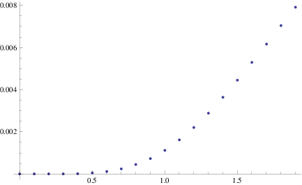
which may be minimized for for every fixed value of . Fig. 6 represents this minimizing value of as the numerical function of .

We find the variationally improved surface eq. (25) and its area as given by eq. (27) for each for the corresponding . For a selection of values for with step size , the dimension less decrease in area of surface of eq. (12) can be seen in the Fig. 7 and interpolating curve of the same is provided in Fig. 8.

VI Conclusions
We have discussed a technique to reduce the area of a surface eq. (11) obtaining variationally improved surface of eq. (25). This algorithm is first applied to a non- minimal surface spanning a boundary for which minimal surface is known namely hemiellipsoid eq. (32). The dimensionless decrease in the area of the hemiellipsoid eq. (32) for different values of and is (see Fig. 5) depending upon how much it is far from the minimal surface, namely the elliptic disk. This shows our algorithm eq. (25) can significantly reduce area of surface that is far from being minimal. After noting this effectiveness, we applied this technique to reduce the area of a surface of eq. (12) bilinearly spanned by four non-planar boundary lines, a special case of Coons patch eq. (11), along with the configuration eq. (17), for a selection of values for with step size . This gave us a much lesser ( in the range to ) dimensionless decrease in less area of surface of eq. (12), as seen in the Fig. 7 or Fig. 8. This suggests that is already a near minimal surface.
References
- [1] X. Jiao, D. Wang, and H. Zha. Simple and effective variational optimization of surface and volume triangulations. Engineering with Computers, 27:81–94, 2011.
- [2] G. Peyré and L. D. Cohen. Geodesic Methods for Shape and Surface Processing, volume 13, chapter Advances in Computational Vision and Medical Image Processing: Methods and Applications, pages 29–56. Springer, 2008.
- [3] Wen-Haw Chen. Improvement of the shortest path problem with geodesic-like method. World Academy of Science, Engineering Technology, 58:689–692, 2011.
- [4] Cai-Yun Li, Ren-Hong Wang, and Chun-Gang Zhu. Designing approximation minimal parametric surfaces with geodesics. Applied Mathematical Modelling, 37:6415 – 6424, 2013.
- [5] R. Osserman. A survey of Minimal Surfaces. Dover Publications Inc., 1986.
- [6] J. C. C. Nitsche. Lectures on Minimal Surfaces. Cambridge University Press, 1989.
- [7] H.A. Schwarz. Gesammelte Mathematische Abhandlungen. 2 Bände. Springer, 1890.
- [8] J. Douglas. Solution of the problem of Plateau. Trans. Amer. Math. Soc., 33(1):263–321, 1931.
- [9] T. Radó. On Plateau’s problem. Ann. Of Math., (2)31(3):457–469, 1930.
- [10] J. Monterde. Bézier surfaces of minimal area: The Dirichlet approach. Computer Aided Geometric Design, 21:117–136, 2004.
- [11] R. Garnier. Le problème de Plateau. Annales Scientifiques de l’E.N.S., 3(45):53–144, 1928.
- [12] L. Tonelli. Sul problema di Plateau, I & II. Rend. R. Accad. dei Lincei, 24:333–339, 393–398, 1936.
- [13] R. Courant. Plateau’s problem and Dirichlet’s principle. Ann. of Math., 38:679–725, 1937.
- [14] R. Courant. Dirichlet’s principle, conformal mapping and minimal surfaces. Springer, 1977.
- [15] C. B. Morrey. The problem of Plateau on a Riemannian manifold. Ann. of Math., (2)49:807–851, 1948.
- [16] C. B. Morrey. The higher-dimensional Plateau problem on a Riemannian manifold. Proc. Nat. Acad. Sci. U.S.A., 54:1029–1035, 1965.
- [17] E. J. Shane. Parameterization of saddle surfaces, with applications to the problem of Plateau. Trans. Amer. Math. Soc., 35:716–733, 1933.
- [18] M. Shiffman. The Plateau problem for non-relative minima. Annals of Math., 40:834–854, 1939.
- [19] Morse and Tompkins. Minimal surfaces of non-minimum type by a new mode of aproximation. Annals of Math., 42:443–472, 1941.
- [20] R. Osserman. A proof of the regularity everywhere of the classical solution to Plateau’s problem. Annals of Math., 91:550–569, 1970.
- [21] R. Gulliver. Regularity of minimizing surfaces of prescribed mean curvature. Annals of Math., 97:275–305, 1973.
- [22] H. Karcher. The triply periodic minimal surfaces of A. Schoen and their constant mean curvature companions. Man. Math., 64:291, 1989.
- [23] Xiao-Diao Chen, Gang Xua, and Yigang Wanga. Approximation methods for the Plateau-Bézier problem. In Computer-Aided Design and Computer Graphics, 2009. CAD/Graphics ’09. 11th IEEE International Conference on, pages 588–591, 2009.
- [24] Gang Xu and Guo zhao Wang. Quintic parametric polynomial minimal surfaces and their properties. Differential Geometry and its Applications, 28:697 – 704, 2010.
- [25] Yong-Xia Hao, Ren-Hong Wang, and Chong-Jun Li. Minimal quasi-Bézier surface. Applied Mathematical Modelling, 36:5751 – 5757, 2012.
- [26] J. M. Richard. Non-abelian dynamics and heavy multiquarks, steiner-tree confinement in hadron spectroscopy. Few Body Syst, 50:137–143, 2011.
- [27] Y. Simonov. Dynamics of confined gluons. Physics of Atomic Nuclei, 68(8):1294–1302, 2005.
- [28] T. J. Allen, M. G. Olsson, and S. Veseli. Curved QCD string dynamics. Phys. Rev. D., 60.074026, 1999.
- [29] N. Brambilla and A. Vairo. Heavy quarkonia: Wilson area law, stochastic vacuum model and dual QCD. Phys. Rev. D., 55:3974–3986, 1997.
- [30] A. M. Green and J. Paton. Quark rearrangement amplitudes in the flux tube model. Nuclear Physics A, 492:595–606, 1989.
- [31] A. M. Green, G. Q. Liu, and S. Wychech. Meson-meson scattering via multi-plaquette interaction. Nuclear Physics A, 509:687–716, 1990.
- [32] S. Furui and B. Masud. On the colour confinement and the minimal surface. Confinement 2000 proceedings, March 2000 arXiv:hep-lat/0006003v1, pages 337–340, 2000.
- [33] S. Furui, A.M. Green, and B. Masud. An analysis of four-quark energies in SU(2) lattice Monte Carlo using the flux tube symmetry. Nucl. Phys. A, pages 582–682, 1995.
- [34] N. Brambilla, E. Montaldi, and G. M. Prosperi. Bethe-Salpeter equation in QCD. Phys.Rev.D, 54:3506–3525, 1996.
- [35] Z. Jaskólsk and K. A. Meissner. Static quark potential from the Polyakov sum over surfaces. Nucl. Phy. B, 418(3):456–476, 1994.
- [36] M. Creutz. Quarks, Gluons and Lattices. Cambridge University Press, 1983.
- [37] N. Brambilla, P. Consoli, and G. M. Prosperi. Consistent derivation of the quark-antiquark and three-quark potentials in a Wilson loop context. Phys. Rev. D, 50:5878–5892, 1994.
- [38] G. Farin. Curves and Surfaces for Computer Aided Geometric Design. The Academic Press, USA, 2002.
- [39] I. D. Faux and M. J. Pratt. Computation Geometry for Design and Manufacture. Ellis Harwood Limited, 1979.
- [40] D. Ahmad and B. Masud. A Coons patch spanning a finite number of curves tested for variationally minimizing its area. Abstract and Applied Analysis, 2013, 2013.
- [41] J. Monterde and H. Ugail. A general 4th-order PDE method to generate Bézier surfaces from the boundary. Computer Aided Geometric Design, 23:208 – 225, 2006.
- [42] M. Do Carmo. Differential Geometry of Curves and Surfaces. Prentice Hall, 1976.
- [43] A. Goetz. Introduction to Differential Geometry. Addison Wesley Publishing Company, 1970.
- [44] W. Businger, P. A. Chevalier, N. Droux, and W. Hett. Computing minimal surfaces on a transputer network. Mathematica Journal, 4:70–74, 1994.
- [45] S. Furui and B. Masud. Numerical calculation of a minimal surface using bilinear interpolations and Chebyshev polynomials. arXiv:math-ph/0608043v2, 2007.
- [46] J. Monterde and H. Ugail. A comparative study between biharmonic Bézier surfaces and biharmonic extremal surfaces. International Journal of Computers and Applications, 31(2):90–96, 2009.
- [47] J. Monterde and H. Ugail. On harmonic and biharmonic Bézier surfaces. Computer Aided Geometric Design, 21:697 – 715, 2004.
- [48] G. E. Farin and D. Hansford. Discrete Coons patches. Computer Aided Geometric Design, 16:691–700, 1999.