跳到论文正文
W Papers独立论文阅读器 arXiv:1205.3069 论文正文 计算阅读时间 · 0%
引用这篇论文根据当前论文元数据生成,正式投稿前建议核对。


License: arXiv.org perpetual non-exclusive license
arXiv:1205.3069v1 [hep-th] 14 May 2012

On a family of (1+1)-dimensional scalar field theory models: kinks, stability, one-loop mass shifts

A. Alonso-Izquierdo Affiliation:  Departamento de Matematica Aplicada and IUFFyM, Universidad de Salamanca, SPAIN Affiliation:  Departamento de Fisica Fundamental and IUFFyM, Universidad de Salamanca, SPAIN    J. Mateos Guilarte
Abstract

In this paper we construct a one-parametric family of (1+1)-dimensional one-component scalar field theory models supporting kinks. Inspired by the sine-Gordon and ϕ4\phi^{4} models, we look at all possible extensions such that the kink second-order fluctuation operators are Schrödinger differential operators with Pöschl-Teller potential wells. In this situation, the associated spectral problem is solvable and therefore we shall succeed in analyzing the kink stability completely and in computing the one-loop quantum correction to the kink mass exactly. When the parameter is a natural number, the family becomes the hierarchy for which the potential wells are reflectionless, the two first levels of the hierarchy being the sine-Gordon and ϕ4\phi^{4} models.

1 Introduction

From the very beginning of the surge of solitons in Quantum Field Theory in the mid seventies it was noticed that the second-order kink fluctuation operators in the sine-Gordon and ϕ4\phi^{4} models were respectively the two first members in the hierarchy of Schrödinger operators with “transparent” Pöschl-Teller wells:

K(1)=−d2d​x2+1−2​sech2​x,K(2)=−d2d​x2+4−6​sech2​x.K^{(1)}=-\frac{d^{2}}{dx^{2}}+1-2\,{\rm sech}^{2}x\hskip 28.45274pt,\hskip 28.45274ptK^{(2)}=-\frac{d^{2}}{dx^{2}}+4-6\,{\rm sech}^{2}x\qquad.

In 1975, Christ and Lee in Reference [2] addressed the following natural problem: what should the potential energy densities in the parent field theoretical models be such that the kink second-order fluctuation operators are the other members in the “transparent” PT hierarchy: K(N)=−d2d​x2+N2−N⁡(N+1)​sech2​xK^{(N)}=-\frac{d^{2}}{dx^{2}}+N^{2}-N(N+1)\,{\rm sech}^{2}x, N∈ℕN\in{\mathbb{N}}? These authors found the general answer and described some analytical properties of the ϕK(N)\phi_{K}^{(N)}-kinks and the U(N)​(ϕ)U^{(N)}(\phi)-potentials arising in this kind of model. They also noticed that the parent potentials had branch points at the vacua for N≥3N\geq 3. In 1987, Trullinger and Flesch [3] succeeded in constructing the N∈ℕN\in\mathbb{N} hierarchy by identifying the parent potentials in terms of some specific special functions. These functions are well defined when the field takes values in the interval in the field space between the two vacua. Beyond those points they tried to build the parent potentials by sewing the special functions just mentioned to some well-behaved functions with suitable properties at higher than the vacuum values of the field. The connection between the two zones, however, was at most twice differentiable at the branching points. Nevertheless, they showed that keeping only lowest-order (Gaussian) field fluctuations around the static vacua and kink solutions, the parent potentials are well behaved. This left open the question of computing the one-loop mass quantum corrections to the kinks associated with these parent potentials. In 1989 Boya and Casahorran applied the procedure of Cahill, Comtet and Glauber [4] to the models in this hierarchy. Thus, they computed the one-loop kink mass quantum correction in terms of the bound state eigenvalues of the K(N)K^{(N)} operator, see [5]. We stress that this formula is valid only if the potential well is reflectionless and suitably integrable.

In a almost parallel development, the problem of the computation of the one-loop mass shifts for the sine-Gordon soliton and ϕ4\phi^{4} kink was addressed. The first to tackle this were Dashen, Hasslacher and Neveu in 1974 in the framework of the ℏ\hbar-expansion of these (1+1)-dimensional field theories [6, 7, 8]. After a zero-point renormalization, which is performed by means of a mode-by-mode subtraction of the eigenvalues of the second-order fluctuation operators valued respectively on the kink and vacuum solutions and a subsequent mass renormalization, the authors derived the so-called first DHN formula. We stress that the DHN formula is again only valid when the kink second-order fluctuation operator is a reflectionless differential operator. In this case, both the kink and vacuum Hessians have a half-bound state whose contributions to the quantum correction annihilate each other in the mode-number cut-off regularization. In reference [9], the authors construct a generalized DHN formula which works smoothly when applied to quite general Scho¨\ddot{\rm o}dinger operators. At the end of the past century a revival in the interest in this problem took place mainly due to ro^\hat{\rm o}le played by quantum solitons in supersymmetric theories. Many subtleties of the regularization/renormalization procedures involved were clarified, starting with the papers [10, 11, 12, 13]. Other related works, [14, 15, 16], addressed mixed issues in the problem by using different types of boundary conditions - PBC, Dirichlet, Robin-, regularization methods -energy cutoff, mode-number cutoff, high-derivatives-, and/or performed phase-shift analysis, in connection with possible modifications due to the quantum effects of the central charge of the SUSY algebra [17, 18]. In parallel, topological defect quantum fluctuations have been studied within the general framework of quantum vacuum fluctuations in recent years and the application of spectral heat kernel/zeta function regularization methods in this kind of problems has grown very effectively, see [19].

In the present paper, however, we address a two-fold goal:

  1. 1.

    We extend the analysis to the case where the parameter σ\sigma of the Pöschl-Teller well is a positive real number, rather than a natural number,

    K(σ)=−d2d​x2+σ2−σ⁡(σ+1)​sech2​xK^{(\sigma)}=-\frac{d^{2}}{dx^{2}}+\sigma^{2}-\sigma(\sigma+1)\,{\rm sech}^{2}x (1)

    descending to the Christ-Lee-Trullinger-Flesch-Boya-Casahorran hierarchy when σ=N∈ℕ\sigma=N\in\mathbb{N}. We shall find analytically the kink solutions, which satisfy intriguing recurrence relations, in the form of regularized incomplete Beta functions.

  2. 2.

    We compute the one-loop kink mass shifts by a variety of methods, depending on the difficulty of the problem. For σ=N∈ℕ\sigma=N\in\mathbb{N} the Cahill-Comtet-Glauber (CCG) formula [4] is applicable but we shall also compute the quantum correction by the Dashen-Hasslacher-Neveu (DHN) mode-number cut-off regularized formula [6] and/or the exact heat kernel/zeta function regularization method [20]. If σ\sigma is not an integer, only the generalized DHN procedure as explained in [9] can be applied. Alternatively, the asymptotic expansion of the heat kernel will allow us to obtain sufficiently good approximations to the one-loop kink mass quantum correction.

The organization of the paper is as follows: in Section §. 2 we shall construct the family of models and we shall also identify the different kinks, discussing interesting relationships between the kinks in different models of the family. We shall also study kink stability, which by construction reduces to the spectral analysis of the operator (1). In Section §. 3 we shall compute the one-loop quantum correction to the kink masses. We shall distinguish the cases σ∈ℕ\sigma\in\mathbb{N} and σ∉ℕ\sigma\notin\mathbb{N}, or equivalently, we shall deal with the Hessian operator (1) with reflection and reflectionless potential well separately. We shall approach this calculation from different points of view. In particular, we shall use the CCG (Cahill, Comtet and Glauber) formula, the DHN (Dashen, Hasslacher and Neveu) formula, the spectral zeta function regularization method and the asymptotic approach. The first three methods can only be applied to models that involve reflectionless Hessian operators, although the second one has been generalized in reference [9]. A comparison between the results obtained with the different methods will be offered, showing a high level of accuracy. In the last Section we shall summarize our conclusions.

2 The family of models: kinks and their stability

2.1 Generalities

The action governing the dynamics in our (1+1)-dimensional relativistic one-scalar field theoretical models is of the form 11 1 The conventions are those set out in reference [21].:

S~​[ψ]=∫∫⁡d​y0​d​y1​(12​∂ψ∂yμ⋅∂ψ∂yμ−U~​[ψ⁡(yμ)]).\tilde{S}[\psi]=\int\!\!\int\,dy^{0}dy^{1}\,\left(\frac{1}{2}\frac{\partial\psi}{\partial y_{\mu}}\cdot\frac{\partial\psi}{\partial y^{\mu}}-\tilde{U}[\psi(y^{\mu})]\right)\quad.

Here, ψ⁡(yμ):ℝ1,1→ℝ\psi(y^{\mu}):\mathbb{R}^{1,1}\rightarrow\mathbb{R} is a real scalar field; i.e., a continuous map from the (1+1)(1+1)-dimensional Minkowski space-time to the field of the real numbers. y0=τy^{0}=\tau and y1=yy^{1}=y are local coordinates in ℝ1,1{\mathbb{R}}^{1,1}, which is equipped with a metric tensor gμ​ν=diag⁡(1,−1),μ,ν=0,1g_{\mu\nu}={\rm diag}(1,-1),\mu,\nu=0,1 such that yμ​yμ=gμ​ν​yμ​yνy_{\mu}y^{\mu}=g^{\mu\nu}y_{\mu}y_{\nu}, ∂∂yμ.∂∂yμ=gμ​ν​∂∂yμ.∂∂yν\frac{\partial}{\partial y_{\mu}}.\frac{\partial}{\partial y^{\mu}}=g^{\mu\nu}\frac{\partial}{\partial y_{\mu}}.\frac{\partial}{\partial y_{\nu}}.

We shall work in a system of units where the speed of light is set to one, c=1c=1, but we shall keep the Planck constant ℏ\hbar explicit because we shall search for one-loop corrections, proportional to ℏ\hbar, to the classical kink masses. In this system, the physical dimensions are:

[ℏ]=[S~]=M​L,[yμ]=L,[ψ]=M12​L12,[U~]=M​L−1.[\hbar]=[\tilde{S}]=ML\quad,\quad[y_{\mu}]=L\quad,\quad[\psi]=M^{\frac{1}{2}}L^{\frac{1}{2}}\quad,\quad[\tilde{U}]=ML^{-1}\quad.

The models that we shall consider are distinguished by different choices of the part of the potential energy density which is independent on the field spatial derivatives: U~​[ψ​(yμ)]\tilde{U}[\psi(y^{\mu})]. In all of them there will be two special parameters, mdm_{d} and γd\gamma_{d}, to be determined in each case, carrying the physical dimensions: [md]=L−1[m_{d}]=L^{-1} and [γd]=M−12​L−12[\gamma_{d}]=M^{-\frac{1}{2}}L^{-\frac{1}{2}}. We define the non-dimensional coordinates, fields and potential in terms of these parameters:

xμ=mdyμ,x0=t,x1=x,ϕ=γdψ,U(ϕ)=γd2md2U~(ψ).x_{\mu}=m_{d}y_{\mu}\,\,\,,\,\,\,x_{0}=t\,\,,\,\,x_{1}=x\quad,\quad\phi=\gamma_{d}\psi\qquad,\qquad U(\phi)=\frac{\gamma_{d}^{2}}{m_{d}^{2}}\tilde{U}(\psi)\qquad.

The action S~​[ψ]\tilde{S}[\psi] is also proportional to a non-dimensional action, i.e., S~​[ψ]=1γd2​S​[ϕ]\tilde{S}[\psi]=\frac{1}{\gamma_{d}^{2}}S[\phi], where

S⁡[ϕ]=∫d​x2​[12​∂μϕ​∂μϕ−U⁡(ϕ)].S[\phi]=\int dx^{2}\left[\frac{1}{2}\partial_{\mu}\phi\,\partial^{\mu}\phi-U(\phi)\right]\qquad. (2)

Here ϕ⁡(xμ):ℝ1,1→ℝ\phi(x_{\mu}):\mathbb{R}^{1,1}\rightarrow\mathbb{R} is a non-dimensional real scalar. Also, we define a non-dimensional potential energy functional by means of the relationship E⁡[ϕ]E[\phi], where

E⁡[ϕ]=γd2md​E~​[ψ],E⁡[ϕ]=∫−∞∞d​x​ε​(x)=∫−∞∞d​x​[12​(∂ϕ∂x)2+U⁡(ϕ)].E[\phi]=\frac{\gamma_{d}^{2}}{m_{d}}\tilde{E}[\psi]\quad,\quad E[\phi]=\int_{-\infty}^{\infty}\,dx\,\varepsilon(x)=\int_{-\infty}^{\infty}\,dx\,\left[\frac{1}{2}\left(\frac{\partial\phi}{\partial x}\right)^{2}+U(\phi)\right]\quad. (3)

From now on we shall work in this non-dimensional context. We shall assume that U⁡(ϕ)U(\phi) is a non-negative twice continuously differentiable function of ϕ∈ℝ\phi\in\mathbb{R}, i.e., U​(ϕ)∈C2​(ℝ)U(\phi)\in C^{2}({\mathbb{R}}) and U⁡(ϕ)≥0U(\phi)\geq 0. We now want to construct kink supporting models where the kink stability is governed by Pöschl-Teller spectral problems. We shall thus assume that the U⁡(ϕ)U(\phi) has at least two minima -which can be fixed as the zeroes of U⁡(ϕ)U(\phi)- at the values ϕ=±1\phi=\pm 1. This assumption does not imply a loss of generality because a translation of the origin and a dilatation in the field space allows us to set this prescription in an arbitrary model.

The configuration space 𝒞{\cal C} of the system is the set of the maps from the spatial line ℝ\mathbb{R} to the internal (field) space ℝ\mathbb{R} for a fixed time tt, such that the energy functional E⁡[ϕ]E[\phi] is finite, 𝒞={ϕ⁡(t,x)∈Maps⁡(ℝ1,ℝ):E⁡[ϕ]<∞}{\cal C}=\{\phi(t,x)\in{\rm Maps}(\mathbb{R}^{1},\mathbb{R}):E[\phi]<\infty\}. The search for kinks is tantamount to the search for finite energy static solutions ϕ⁡(x)\phi(x) of the field equations, which in this case become the “Newton” ODE:

d2​ϕd​x2=∂U∂ϕ.\frac{d^{2}\phi}{dx^{2}}=\frac{\partial U}{\partial\phi}\qquad. (4)

A Lorentz transformation shows the static solution ϕ⁡(x)\phi(x) in its center of mass as the traveling wave: ϕ⁡(t,x)=ϕ⁡(x−v​t1−v2)\phi(t,x)=\phi(\frac{x-vt}{\sqrt{1-v^{2}}}). Moreover, spatial translations and reflections, x→x+x0x\rightarrow x+x_{0}, x↦−xx\mapsto-x, provide more solutions because of the invariance of (4) with respect to these transformations. Therefore, the complete family of solitary wave solutions of (4) is compactly written as: ϕ⁡(x¯)\phi(\overline{x}), x¯=(−1)a​x−x0−v​t1−v2\overline{x}=(-1)^{a}\frac{x-x_{0}-vt}{\sqrt{1-v^{2}}} with a=0,1a=0,1.

The second-order ODE (4) always admits the “mechanical energy” I1=12​(d​ϕd​x)2−U⁡(ϕ)I_{1}=\frac{1}{2}\left(\frac{d\phi}{dx}\right)^{2}-U(\phi) as a first integral. Because the “mechanical action” is the field theoretical energy, the energy finiteness requirement identifies the kink solutions as the trajectories of I1=0I_{1}=0 mechanical energy:

d​ϕd​x=±2​U​(ϕ).\frac{d\phi}{dx}=\pm\sqrt{2U(\phi)}\qquad. (5)

Therefore, the kink solutions interpolate between the ϕV=∓1\phi_{V}=\mp 1 vacuum at x=−∞x=-\infty and the ϕV=±1\phi_{V}=\pm 1 vacuum at x=+∞x=+\infty:

limx→−∞ϕK​(t,x)=∓1∈ℳ,limx→+∞ϕK​(t,x)=±1∈ℳ.\lim_{x\rightarrow-\infty}\phi_{K}(t,x)=\mp 1\in{\cal M}\qquad,\qquad\lim_{x\rightarrow+\infty}\phi_{K}(t,x)=\pm 1\in{\cal M}\qquad.

From the signs in the equation (5) one sees that the interpolation is monotonic: the kink solutions are either monotonically increasing (kinks) or decreasing (anti-kinks) functions of xx from ∓1\mp 1 at the left boundary of the line to ±1\pm 1 on the opposite spatial limit.

The linear stability analysis of any static solution - vacua ϕV\phi_{V} or kink ϕK​(x)\phi_{K}(x)- is codified by the spectral problems K0​fω0​(x)=ω02​fω0​(x)K_{0}f_{\omega_{0}}(x)=\omega_{0}^{2}f_{\omega_{0}}(x) and K​fω​(x)=ω2​fω​(x)Kf_{\omega}(x)=\omega^{2}f_{\omega}(x) for the associated second-order fluctuation (Hessian) operators:

K0=−d2d​x2+∂2U∂ϕ2​[ϕV],K=−d2d​x2+∂2U∂ϕ2​[ϕK​(x)].K_{0}=-\frac{d^{2}}{dx^{2}}+\frac{\partial^{2}U}{\partial\phi^{2}}[\phi_{V}]\quad,\quad K=-\frac{d^{2}}{dx^{2}}+\frac{\partial^{2}U}{\partial\phi^{2}}[\phi_{K}(x)]\quad. (6)

The stability of the solutions ϕV\phi_{V} and ϕK​(x)\phi_{K}(x) is guaranteed when the eigenvalues of these operators are non-negative. In particular, we are interested in the “parent” potentials that admit kink solutions such that:

K(σ)=−d2d​x2+σ2−σ⁡(σ+1)​sech2​x¯,K^{(\sigma)}=-\frac{d^{2}}{dx^{2}}+\sigma^{2}-\sigma(\sigma+1)\,{\rm sech}^{2}\overline{x}\quad, (7)

where σ∈ℝ\sigma\in\mathbb{R}. The potential wells associated with these operators V(σ)​(x¯)=−σ⁡(σ+1)​sech2​x¯V^{(\sigma)}(\overline{x})=-\sigma(\sigma+1)\,{\rm sech}^{2}\overline{x} are depicted in Figure 1 where the integer values of σ\sigma has been emphasized. Note that the wells become deeper and higher as σ\sigma increases.

Refer to caption          Refer to caption

Figure 1: Graphical representations of: (a) the potential well in the Hessian operator for several values of σ\sigma (b) the kink profiles for several values of σ\sigma. The cases σ=N\sigma=N have been emphasized.

We shall denote by ϕK(σ)​(x¯)\phi_{K}^{(\sigma)}(\overline{x}) the kink solutions and by U(σ)​(ϕ)U^{(\sigma)}(\phi) the parent potential for a given σ\sigma in this family of models. Because the kink solutions asymptotically reach the vacuum values ϕV(σ)=±1\phi^{(\sigma)}_{V}=\pm 1, the kink Hessian operators are accompanied by the vacuum Hessians:

K0(σ)=−d2d​x2+σ2.K^{(\sigma)}_{0}=-\frac{d^{2}}{dx^{2}}+\sigma^{2}\quad.

Thus, the mass of the fundamental quanta in these models is: ∂2U∂ϕ2​[ϕV]=σ2\frac{\partial^{2}U}{\partial\phi^{2}}[\phi_{V}]=\sigma^{2}.

2.2 Zero modes and kinks

Our first task is the identification of the parent potentials such that:

d2​U(σ)d​ϕ2​[ϕK(σ)​(x¯)]=σ2−σ⁡(σ+1)​sech2​x¯.\frac{d^{2}U^{(\sigma)}}{d\phi^{2}}[\phi_{K}^{(\sigma)}(\overline{x})]=\sigma^{2}-\sigma(\sigma+1)\,{\rm sech}^{2}\overline{x}\qquad. (8)

The solution of (8) seems hopeless without knowledge of ϕK(σ)​(x¯)\phi_{K}^{(\sigma)}(\overline{x}). The equation (5)

d​ϕK(σ)d​x¯=2​U(σ)​(ϕK(σ)),\frac{d\phi_{K}^{(\sigma)}}{d\overline{x}}=\sqrt{2U^{(\sigma)}(\phi_{K}^{(\sigma)})}\qquad, (9)

however, does allow us to interpret (8) as an ODE in the x¯\overline{x} variable via the change of variables from ϕ\phi to x¯\overline{x}. Recall that ϕK(σ):ℝ→[−1,1]\phi_{K}^{(\sigma)}:\mathbb{R}\rightarrow[-1,1], x¯↦ϕK(σ)​(x¯)\overline{x}\mapsto\phi_{K}^{(\sigma)}(\overline{x}) is a bijective map determined by equation (9). Trading the implicit parent potential for the kink solutions by the explicit function of x¯\overline{x} 𝔘σ​(x¯)=U(σ)​(ϕK(σ)​(x¯))\mathfrak{U}_{\sigma}(\overline{x})=U^{(\sigma)}(\phi_{K}^{(\sigma)}(\overline{x})) and bearing in mind from equation (5) that d​U(σ)d​ϕ=12​𝔘σ​d​𝔘σd​x¯\frac{dU^{(\sigma)}}{d\phi}=\frac{1}{\sqrt{2\mathfrak{U}_{\sigma}}}\frac{d\mathfrak{U}_{\sigma}}{d\overline{x}} and d2​U(σ)d​ϕ2=12​𝔘σ​d2​𝔘σd​x¯2−1(2​𝔘σ)2​(d​𝔘σd​x¯)2\frac{d^{2}U^{(\sigma)}}{d\phi^{2}}=\frac{1}{2\mathfrak{U}_{\sigma}}\frac{d^{2}\mathfrak{U}_{\sigma}}{d\overline{x}^{2}}-\frac{1}{(2\mathfrak{U}_{\sigma})^{2}}(\frac{d\mathfrak{U}_{\sigma}}{d\overline{x}})^{2}, the equation (8) becomes:

12​𝔘σ​(x¯)​d2​𝔘σd​x¯2−1(2​𝔘σ​(x¯))2​(d​𝔘σd​x¯)2=σ2−σ⁡(σ+1)​sech2​x¯.\frac{1}{2\mathfrak{U}_{\sigma}(\overline{x})}\frac{d^{2}\mathfrak{U}_{\sigma}}{d\overline{x}^{2}}-\frac{1}{(2\mathfrak{U}_{\sigma}(\overline{x}))^{2}}\left(\frac{d\mathfrak{U}_{\sigma}}{d\overline{x}}\right)^{2}=\sigma^{2}-\sigma(\sigma+1)\,{\rm sech}^{2}\overline{x}\qquad. (10)

(8) is a non-linear ordinary differential equation that can easily be reduced to the Riccati equation by means of the change F⁡(x)=12​log⁡𝔘σF(x)=\frac{1}{2}\log\mathfrak{U}_{\sigma}:

d2​Fd​x¯2+(d​Fd​x¯)2=σ2−σ⁡(σ+1)​sech2​x¯.\frac{d^{2}F}{d\overline{x}^{2}}+\left(\frac{dF}{d\overline{x}}\right)^{2}=\sigma^{2}-\sigma(\sigma+1)\,{\rm sech}^{2}\overline{x}\quad.

A particular solution can be obtained by the standard procedure of sending the Riccati equation to the Schro¨\ddot{\rm o}dinger equation via the new change d​Fd​x=d​log⁡ψ0d​x\frac{dF}{dx}=\frac{d\log\psi_{0}}{dx}, or, 𝔘=ψ02\mathfrak{U}=\psi_{0}^{2}:

d2​ψ0d​x¯2=(σ2−σ⁡(σ+1)​sech2​x¯)​ψ0,\frac{d^{2}\psi_{0}}{d\overline{x}^{2}}=\left(\sigma^{2}-\sigma(\sigma+1){\rm sech}^{2}\overline{x}\right)\psi_{0}\qquad, (11)

i.e., ψ0​(x¯)=Cσ​sechσ​(x¯)\psi_{0}(\overline{x})=\sqrt{C_{\sigma}}{\rm sech}^{\sigma}(\overline{x}) is the ground state of zero energy in the PT potential well. Therefore, we find a solution depending on the integration constant CσC_{\sigma} of our problem:

𝔘σ​(x¯)=Cσ​sech2​σ​x¯,limx¯→±∞𝔘σ​(x¯)=0.\mathfrak{U}_{\sigma}(\overline{x})=C_{\sigma}\,{\rm sech}^{2\sigma}\overline{x}\quad,\quad\lim_{\overline{x}\rightarrow\pm\infty}\mathfrak{U}_{\sigma}(\overline{x})=0\qquad. (12)

This solution fits smoothly into our scheme because the kinks tend to the zeroes of the potential U(σ)​(ϕ)U^{(\sigma)}(\phi) at x=±∞x=\pm\infty. The hidden reason for finding this expression (12) for the parent potential as a function of the parameter x¯\overline{x} is that via the equation

d​ϕK(σ)=2​𝔘σ​(x¯)​d​x¯d\phi_{K}^{(\sigma)}=\sqrt{2\,\mathfrak{U}_{\sigma}(\overline{x})}d\overline{x} (13)

the potential is related to the translational mode d​ϕK(σ)d​x¯\frac{d\phi_{K}^{(\sigma)}}{d\overline{x}}, which is in turn the ground state of zero energy of K(σ)K^{(\sigma)} because of general arguments (just plug it in (4)). Integration of (13) immediately produces the kink solution

ϕK(σ)​(x¯)=2​Γ​[12+σ2]π​Γ​[σ2]​tanh⁡x¯​F12​[12,1−σ2,32,tanh2⁡x¯]\phi_{K}^{(\sigma)}(\overline{x})=\frac{2\Gamma[\frac{1}{2}+\frac{\sigma}{2}]}{\sqrt{\pi}\Gamma[\frac{\sigma}{2}]}\tanh\overline{x}\,\,{}_{2}F_{1}[{\textstyle\frac{1}{2},1-\frac{\sigma}{2},\frac{3}{2},\tanh^{2}\overline{x}}] (14)

in terms of a Gauss hypergeometric function. The constant CσC_{\sigma} has been tuned to

Cσ=2​Γ​[12+σ2]2π​Γ​[σ2]2C_{\sigma}=\frac{2\Gamma[\frac{1}{2}+\frac{\sigma}{2}]^{2}}{\pi\Gamma[\frac{\sigma}{2}]^{2}}

in order to set the zeroes of the parent potential at the ϕ=±1\phi=\pm 1 values. One can check that for σ=1\sigma=1 the soliton of the sine-Gordon model ϕK(1)​(x¯)=4π​arctan⁡tanh⁡x¯2\phi_{K}^{(1)}(\overline{x})=\frac{4}{\pi}\arctan\tanh\frac{\overline{x}}{2} is found, whereas the kink of the ϕ4\phi^{4} model ϕK(2)​(x¯)=tanh⁡x¯\phi_{K}^{(2)}(\overline{x})=\tanh\overline{x} arises when σ=2\sigma=2.

It is convenient to rewrite the kink profile (14) using other special functions. We recall the definition of the beta function in terms of three Gauss Gamma functions: B⁡(a,b)=∫01ta−1​(1−t)b−1​𝑑t=Γ⁡[a]​Γ​[b]Γ⁡[a+b]B(a,b)=\int_{0}^{1}t^{a-1}(1-t)^{b-1}dt=\frac{\Gamma[a]\Gamma[b]}{\Gamma[a+b]}. We also need the incomplete beta function B⁡(z,a,b)B(z;a,b) of a free upper integration limit z∈[0,1]z\in[0,1]: B⁡(z,a,b)=∫0xta−1​(1−t)b−1​𝑑t=1a​za​F12​[a,1−b,a+1,z]B(z;a,b)=\int_{0}^{x}t^{a-1}(1-t)^{b-1}dt=\frac{1}{a}z^{a}\,{}_{2}F_{1}[a,1-b,a+1,z], which is related to the hypergeometric Gauss function. Finally, we shall consider the regularized incomplete beta function I⁡(z,a,b)=B⁡(z,a,b)B⁡(a,b)I(z;a,b)=\frac{B(z;a,b)}{B(a,b)}. With this arsenal we obtain the very compact formula:

ϕK(σ)​(x¯)=sign⁡(x¯)​I​[tanh2⁡x¯;12,σ2].\phi_{K}^{(\sigma)}(\overline{x})={\rm sign}(\overline{x})\,\,I[\textstyle\tanh^{2}\overline{x};\frac{1}{2},\frac{\sigma}{2}]\quad. (15)

Note that formula (15) is an odd function because of the sign function that multiplies I⁡[tanh2⁡x¯;12,σ2]I[\textstyle\tanh^{2}\overline{x};\frac{1}{2},\frac{\sigma}{2}]. This does not induce singularities because II is zero at the origin, see Figure 2. It is remarkable that the soliton and kink solutions are embraced in this general formula.

2.3 Recurrence relations

The magic of the hypergeometric functions gives rise to interesting recurrence relations between kinks for different values of σ\sigma from (14). The well-known formula F12​[a,b+1,c,z]=F12​[a,b,c,z]+zb​dd​z​F12​[a,b,c,z]{}_{2}F_{1}[a,b+1,c,z]={}_{2}F_{1}[a,b,c,z]+\frac{z}{b}\frac{d}{dz}{}_{2}F_{1}[a,b,c,z] applied in (14) means that:

ϕK(σ+2)​(x¯)=ϕK(σ)​(x¯)+1σ​tanh⁡x¯​d​ϕK(σ)d​x¯​(x¯),\phi_{K}^{(\sigma+2)}(\overline{x})=\phi_{K}^{(\sigma)}(\overline{x})+\frac{1}{\sigma}\tanh\overline{x}\,\frac{d\phi_{K}^{(\sigma)}}{d\overline{x}}(\overline{x})\quad, (16)

a relation between the σ\sigma and σ+2\sigma+2 kink profiles. Taking into account (13) we rewrite (16) as:

ϕK(σ+2)​(x¯)=ϕK(σ)​(x¯)+2​Γ​[12+σ2]σ​π​Γ​[σ2]​tanh⁡x¯​sechσ​x¯,\phi_{K}^{(\sigma+2)}(\overline{x})=\phi_{K}^{(\sigma)}(\overline{x})+\frac{2\Gamma[\frac{1}{2}+\frac{\sigma}{2}]}{\sigma\sqrt{\pi}\Gamma[\frac{\sigma}{2}]}\tanh\overline{x}\,{\rm sech}^{\sigma}\overline{x}\quad, (17)

a form of the recurrence relations that can also be derived from the identities between regularized beta functions: I⁡(z,a,b)=1−I⁡(1−z,b,a)I(z,a,b)=1-I(1-z,b,a) and I⁡(z,a+1,b)=I⁡(z,a,b)−za​(1−z)ba​B​(a,b)I(z,a+1,b)=I(z,a,b)-\frac{z^{a}(1-z)^{b}}{aB(a,b)}, applied in the formula (15). In formula (17) one notices that the (σ+2)(\sigma+2)-kink is equal to the addition of the σ\sigma-kink plus an odd function, implying that |ϕK(σ+2)​(x¯)|≥|ϕK(σ)​(x¯)||\phi_{K}^{(\sigma+2)}(\overline{x})|\geq|\phi_{K}^{(\sigma)}(\overline{x})|. Therefore, the kink profile is more and more concentrated around its center in members of the family with higher and higher σ\sigma, see Figure 1(b).

For odd and even integer values of σ\sigma the formulas simplify analytically. We discuss the σ=2​k\sigma=2k even and σ=2​k+1\sigma=2k+1 odd, k∈ℕk\in\mathbb{N}, cases separately. If σ=2​k\sigma=2k, (17) becomes:

ϕK(2​k+2)​(x¯)=ϕK(2​k)​(x¯)+(2​k−1)!!2k​k!​tanh⁡x¯​sech2​k​x¯.\phi_{K}^{(2k+2)}(\overline{x})=\phi_{K}^{(2k)}(\overline{x})+\frac{(2k-1)!!}{2^{k}k!}\tanh\overline{x}\,{\rm sech}^{2k}\overline{x}\quad.

In the odd case the same recurrence relation reads:

ϕK(2​k+3)​(x¯)=ϕK(2​k+1)​(x¯)+2k+1​(k+1)!π⁡(2​k+1)!!​tanh⁡x¯​sech2​k+1​x¯.\phi_{K}^{(2k+3)}(\overline{x})=\phi_{K}^{(2k+1)}(\overline{x})+\frac{2^{k+1}(k+1)!}{\pi(2k+1)!!}\tanh\overline{x}\,{\rm sech}^{2k+1}\overline{x}\quad.

In Table 1 we show the kink profiles of the first ten members of the hierarchy of models.

σ\sigma ϕK(σ)​(x¯)\phi_{K}^{(\sigma)}(\overline{x}) 1 ϕK(1)​(x¯)=2π​arcsin⁡tanh⁡x¯\phi_{K}^{(1)}(\overline{x})=\frac{2}{\pi}\arcsin\tanh\overline{x} 3 ϕK(3)​(x¯)=ϕK(1)​(x¯)+2π​tanh⁡x¯​sech​x¯\phi_{K}^{(3)}(\overline{x})=\phi_{K}^{(1)}(\overline{x})+\frac{2}{\pi}\tanh\overline{x}\,{\rm sech}\,\overline{x} 5 ϕK(5)​(x¯)=ϕK(3)​(x¯)+43​π​tanh⁡x¯​sech3​x¯\phi_{K}^{(5)}(\overline{x})=\phi_{K}^{(3)}(\overline{x})+\frac{4}{3\pi}\tanh\overline{x}\,{\rm sech}^{3}\overline{x} 7 ϕK(7)​(x¯)=ϕK(5)​(x¯)+1615​π​tanh⁡x¯​sech5​x¯\phi_{K}^{(7)}(\overline{x})=\phi_{K}^{(5)}(\overline{x})+\frac{16}{15\pi}\tanh\overline{x}\,{\rm sech}^{5}\overline{x} 9 ϕK(9)​(x¯)=ϕK(7)​(x¯)+3235​π​tanh⁡x¯​sech7​x¯\phi_{K}^{(9)}(\overline{x})=\phi_{K}^{(7)}(\overline{x})+\frac{32}{35\pi}\tanh\overline{x}\,{\rm sech}^{7}\overline{x}     σ\sigma ϕK(σ)​(x¯)\phi_{K}^{(\sigma)}(\overline{x}) 2 ϕK(2)​(x¯)=tanh⁡x¯\phi_{K}^{(2)}(\overline{x})=\tanh\overline{x} 4 ϕK(4)​(x¯)=ϕK(2)​(x¯)+12​tanh⁡x¯​sech2​x¯\phi_{K}^{(4)}(\overline{x})=\phi_{K}^{(2)}(\overline{x})+\frac{1}{2}\tanh\overline{x}\,{\rm sech}^{2}\overline{x} 6 ϕK(6)​(x¯)=ϕK(4)​(x¯)+38​tanh⁡x¯​sech4​x¯\phi_{K}^{(6)}(\overline{x})=\phi_{K}^{(4)}(\overline{x})+\frac{3}{8}\tanh\overline{x}\,{\rm sech}^{4}\overline{x} 8 ϕK(8)​(x¯)=ϕK(6)​(x¯)+516​tanh⁡x¯​sech6​x¯\phi_{K}^{(8)}(\overline{x})=\phi_{K}^{(6)}(\overline{x})+\frac{5}{16}\tanh\overline{x}\,{\rm sech}^{6}\overline{x} 10 ϕK(10)​(x¯)=ϕK(8)​(x¯)+35128​tanh⁡x¯​sech8​x¯\phi_{K}^{({10})}(\overline{x})=\phi_{K}^{(8)}(\overline{x})+\frac{35}{128}\tanh\overline{x}\,{\rm sech}^{8}\overline{x}

Table 1: Some kink solutions of the hierarchy of models characterized by σ∈ℕ\sigma\in\mathbb{N}.

There also exist recurrence relations between σ\sigma- and σ+1\sigma+1-kinks differing in one unit in the family parameter, although in this case the formula involves a quadrature. From (13) we obtain

d​ϕK(σ+1)=𝔘σ+1​(x¯)𝔘σ​(x¯)​d​ϕK(σ)=σ2​Γ​[σ2]2Γ​[12+σ2]2​sech​x¯​d​ϕK(σ),d\phi_{K}^{({\sigma+1})}=\frac{\sqrt{\mathfrak{U}_{\sigma+1}(\overline{x})}}{\sqrt{\mathfrak{U}_{\sigma}(\overline{x})}}d\phi_{K}^{(\sigma)}=\frac{\sigma}{2}\frac{\Gamma[\frac{\sigma}{2}]^{2}}{\Gamma[\frac{1}{2}+\frac{\sigma}{2}]^{2}}\,{\rm sech}\,\overline{x}\,d\phi_{K}^{(\sigma)}\quad,

which can be two-sided integrated to find:

ϕK(σ+1)​(x¯)=σ2​Γ​[σ2]2Γ​[12+σ2]2​[sech​x¯​ϕK(σ)​(x¯)+∫sech​x¯​tanh⁡x¯​ϕK(σ)​(x¯)​𝑑x¯].\phi_{K}^{(\sigma+1)}(\overline{x})=\frac{\sigma}{2}\frac{\Gamma[\frac{\sigma}{2}]^{2}}{\Gamma[\frac{1}{2}+\frac{\sigma}{2}]^{2}}\left[{\rm sech}\,\overline{x}\,\phi_{K}^{(\sigma)}(\overline{x})+\int{\rm sech}\,\overline{x}\,\tanh\overline{x}\,\phi_{K}^{(\sigma)}(\overline{x})d\overline{x}\right]\quad.

An integration by parts has been performed in the right-hand side member.

The classical energy of the kinks can easily be worked out from the zero modes, the connection formulas between hypergeometric functions and the Kummer theorem:

Eclas​[ϕK(σ)​(x¯)]=∫−∞∞d​x¯​(d​ϕK(σ)d​x¯)2=4σ+1π​σ⋅Γ​[12+σ2]2Γ​[σ+12]2⋅F12​[σ,2​σ,1+σ;−1]=4​Γ​[σ]​Γ​[12+σ2]2π​Γ​[σ+12]​Γ​[σ2]2.E_{\rm clas}[\phi_{K}^{(\sigma)}(\overline{x})]=\int_{-\infty}^{\infty}\,d\overline{x}\,\left(\frac{d\phi_{K}^{(\sigma)}}{d\overline{x}}\right)^{2}=\frac{4^{\sigma+1}}{\pi\sigma}\cdot\frac{\Gamma[\frac{1}{2}+\frac{\sigma}{2}]^{2}}{\Gamma[\sigma+\frac{1}{2}]^{2}}\cdot{}_{2}F_{1}[\sigma,2\sigma,1+\sigma;-1]=\frac{4\Gamma[\sigma]\Gamma[\frac{1}{2}+\frac{\sigma}{2}]^{2}}{\sqrt{\pi}\Gamma[\sigma+\frac{1}{2}]\Gamma[\frac{\sigma}{2}]^{2}}\quad.

2.4 Parent potentials

To completely define the family of models we identify the potential (12) as a function of the field ϕ\phi by, first, inverting formula (15):

x¯=arctanh​I−1​[|ϕK(σ)|;12,σ2]\overline{x}={\rm arctanh}\,\sqrt{I^{-1}\textstyle\left[|\phi_{K}^{(\sigma)}|;\frac{1}{2},\frac{\sigma}{2}\right]}

and, then, plugging this expression into the formula (12) to find:

U(σ)​(ϕ)=2​Γ​[12+σ2]2π​Γ​[σ2]2​(1−I−1​[|ϕ|;12,σ2])σ.U^{(\sigma)}(\phi)=\frac{2\Gamma[\frac{1}{2}+\frac{\sigma}{2}]^{2}}{\pi\Gamma[\frac{\sigma}{2}]^{2}}\left(1-I^{-1}\textstyle\left[|\phi|;\frac{1}{2},\frac{\sigma}{2}\right]\right)^{\sigma}\qquad. (18)

We emphasize that this formula is only valid in the interval ϕ∈[−1,1]\phi\in[-1,1] in the internal space, see Figure 2(a). The reason is that the kink solutions live only in this interval and use of the map ϕK(σ):ℝ→[−1,1]\phi_{K}^{(\sigma)}:\mathbb{R}\rightarrow[-1,1] to reconstruct the potential in (2) is restricted to this interval. Obviously the character of the potential for field configurations such that |ϕ|≥1|\phi|\geq 1 does not influence the kink solutions. We have the freedom, however, to mathematically extend the definition of the potential as a function of ϕ\phi to the |ϕ|≥1|\phi|\geq 1 range. Even requiring twice-differentiable functions U(σ)​(ϕ)∈𝒞2​(ℝ)U^{(\sigma)}(\phi)\in{\cal C}^{2}(\mathbb{R}), there are several possible choices of continuations of U(σ)​(ϕ)U^{(\sigma)}(\phi): see [3] for some examples. In Figure 2(b) we show periodic continuations of the potential defined in ϕ∈[−1,1]\phi\in[-1,1] to the |ϕ|≥1|\phi|\geq 1 half-lines. Here, the piece of UU depicted in the Figure 2(a) is cloned in all the [2​k−1,2​k+1][2k-1,2k+1], k∈ℤk\in\mathbb{Z}, intervals. The continuations depicted in Figure 2(c) are accomplished analytically by expanding U(σ)​(ϕ)=2​Γ​[12+σ2]2π​Γ​[σ2]2​(1−I−1​[|ϕ|;12,σ2])σU^{(\sigma)}(\phi)=\frac{2\Gamma[\frac{1}{2}+\frac{\sigma}{2}]^{2}}{\pi\Gamma[\frac{\sigma}{2}]^{2}}\left(1-I^{-1}\textstyle\left[|\phi|;\frac{1}{2},\frac{\sigma}{2}\right]\right)^{\sigma} as a power series near the ϕ=±1\phi=\pm 1 points and truncating the series to a polynomial at a finite higher than two order.

[Uncaptioned image]       [Uncaptioned image]

Refer to caption       Refer to caption

Figure 2: Graphical representation for the potential: (a) in the range |ϕ|≤1|\phi|\leq 1, (b) periodic continuations, (c) polynomial continuations, (d) σ=4\sigma=4 generalized Chebychev continuation, to |ϕ|≥1|\phi|\geq 1.

Starting from the σ=1\sigma=1 potential in formula (18) extended by the periodic continuation scheme we obtain: U(1)​(ϕ)=1π2​[1+cos⁡(π​ϕ)]U^{(1)}(\phi)=\frac{1}{\pi^{2}}[1+\cos(\pi\phi)], a beautiful version of the sine-Gordon model (properly translated in internal space). Extending the σ=2\sigma=2 potential in (18) by using the second type of continuation we recover the ϕ4\phi^{4} model: U(2)​(ϕ)=12​(ϕ2−1)2U^{(2)}(\phi)=\frac{1}{2}(\phi^{2}-1)^{2}. Indeed, these two examples are the exceptional 𝒞∞​(ℝ){\cal C}^{\infty}(\mathbb{R}) continuations in the whole hierarchy of σ=N\sigma=N potentials. More generally, C3​(ℝ)C^{3}(\mathbb{R}) continuations of the potential (18) are not possible if σ>2\sigma>2 because

d3​U(σ)d​ϕ3=dd​ϕ​[σ2−σ⁡(σ+1)​sech2​x¯]=2​σ​(σ+1)​sech2​x¯​tanh⁡x¯​d​x¯d​ϕ=2​σ​(σ+1)Cσ​sech2−σ​x¯​tanh⁡x¯\frac{d^{3}U^{(\sigma)}}{d\phi^{3}}=\frac{d}{d\phi}\left[\sigma^{2}-\sigma(\sigma+1)\,{\rm sech}^{2}\,\overline{x}\right]=2\sigma(\sigma+1)\,{\rm sech}^{2}\,\overline{x}\tanh\overline{x}\frac{d\overline{x}}{d\phi}=\frac{2\sigma(\sigma+1)}{\sqrt{C_{\sigma}}}\,{\rm sech}^{2-\sigma}\overline{x}\tanh\overline{x}

diverges when x¯\overline{x} tends to infinity (the vacuum points ϕ=±1\phi=\pm 1). There is however another case, σ=4\sigma=4, where the (18) U(4)​(ϕ)=98​[1−2​cos⁡(23​arcsin⁡ϕ)]4U^{(4)}(\phi)=\frac{9}{8}\left[1-2\cos\left(\frac{2}{3}\arcsin\phi\right)\right]^{4} extended to the whole real line ℝ\mathbb{R} can be expressed in terms of elementary functions:

U(4)​(ϕ)={98​[1−2​cos⁡(23​arcsin⁡ϕ)]4 if ​|ϕ|≤198​[1−2​cos⁡(23​arcsin⁡1ϕ)]4 if ​|ϕ|>1.U^{(4)}(\phi)=\left\{\begin{array}[]{ll}\frac{9}{8}\left[1-2\cos\left(\frac{2}{3}\arcsin\phi\right)\right]^{4}&\mbox{ if }|\phi|\leq 1\\ \frac{9}{8}\left[1-2\cos\left(\frac{2}{3}\arcsin\frac{1}{\phi}\right)\right]^{4}&\mbox{ if }|\phi|>1\end{array}\right.\quad. (19)

This function, akin to Chebychev polynomials, is depicted in Figure 2(d) and is easily seen to be 𝒞2​(ℝ){\cal C}^{2}(\mathbb{R}). Note, however, that this continuation differs from that depicted in Figure 2(c), in particular the extended potential tends to 98\frac{9}{8} at ϕ=±∞\phi=\pm\infty.

2.5 Kink stability

We recall that the Hessian differential operator at the vacuum solutions ϕV(σ)=±1\phi_{V}^{(\sigma)}=\pm 1 reads:

K0(σ)=−d2d​x2+∂2U(σ)∂ϕ2​[±1]=−d2d​x2+σ2,K_{0}^{(\sigma)}=-\frac{d^{2}}{dx^{2}}+\frac{\partial^{2}U^{(\sigma)}}{\partial\phi^{2}}[\pm 1]=-\frac{d^{2}}{dx^{2}}+\sigma^{2}\quad,

see (6). In order to analyze the spectrum of this differential operator we temporarily confine the system in an interval of (non dimensional) length ll and impose periodic boundary conditions on the plane eigen-waves ψ0​k(σ)​(x)=1l​e−i​k​x\psi_{0k}^{(\sigma)}(x)=\frac{1}{\sqrt{l}}e^{-ikx}. The wave vectors are quantized k​l=2​π​n,n∈ℤkl=2\pi n,n\in{\mathbb{Z}}, and in the limit of very large ll the spectral density is: ρ⁡(K0(σ))=d​nd​k=l2​π\rho(K_{0}^{(\sigma)})=\frac{dn}{dk}=\frac{l}{2\pi}. The corresponding eigenvalues are ω2​(k)=k2+σ2\omega^{2}(k)=k^{2}+\sigma^{2} such that the threshold of the continuous spectrum arising at l=∞l=\infty is σ2\sigma^{2}. The constant function is also a non-propagating eigen-function of K0(σ)K_{0}^{(\sigma)} with energy σ2\sigma^{2}. Bound states buried in the threshold of the continuous spectrum are called half-bound states because due to the 1D Levinson Theorem must be counted with a weight of one-half. In sum, we have that Spec⁡(K0(σ))={σ2}12∪{k2+σ2}k∈ℝ{\rm Spec}(K_{0}^{(\sigma)})=\{\sigma^{2}\}_{\frac{1}{2}}\cup\{k^{2}+\sigma^{2}\}_{k\in\mathbb{R}}. All the eigenvalues are positive, and there are no tachyonic waves fluctuating around the vacua, which accordingly are stable.

The analysis of kink stability requires us to deal with a more complicated but tractable spectral problem: K(σ)​ψω​(x)=ω2​ψω​(x)K^{(\sigma)}\psi_{\omega}(x)=\omega^{2}\psi_{\omega}(x). We confront the Schrödinger operator

K(σ)=−d2d​x2+v2+V⁡(x)=−d2d​x2+σ2−σ⁡(σ+1)​sech2​x,K^{(\sigma)}=-\frac{d^{2}}{dx^{2}}+v^{2}+V(x)=-\frac{d^{2}}{dx^{2}}+\sigma^{2}-\sigma(\sigma+1)\,{\rm sech}^{2}x\qquad, (20)

i.e., the quantum Hamiltonian describing the motion of a particle of (non-dimensional) mass μ=ℏ2​γd42\mu=\frac{\hbar^{2}\gamma_{d}^{4}}{2} in a x→−xx\to-x symmetric Pöschl-Teller well (7). The scattering eigen-functions of eigenvalue ω2​(k,σ)=k2+σ2\omega^{2}(k;\sigma)=k^{2}+\sigma^{2} are well known [22]:

ψk(σ)​(x)=2i​k​Ck(σ)​sech−i​k​x¯⋅F12​[σ+1−i​k,−σ−i​k,1−i​k,e−x¯ex¯+e−x¯]k∈ℝ.\psi_{k}^{(\sigma)}(x)=2^{ik}C_{k}^{(\sigma)}{\rm sech}^{-ik}\overline{x}\,\,\cdot{}_{2}F_{1}\left[\sigma+1-ik,-\sigma-ik,1-ik,{\textstyle\frac{e^{-\overline{x}}}{e^{\overline{x}}+e^{-\overline{x}}}}\right]\hskip 28.45274ptk\in\mathbb{R}\quad. (21)

These eigen-functions belonging to the continuous spectrum of K(σ)K^{(\sigma)} can also be written in the simpler form

ψk(σ)​(x)=Ck(σ)​ei​k​x¯​F12​[−σ,σ+1,1−i​k,e−x¯ex¯+e−x¯]\psi_{k}^{(\sigma)}(x)=C_{k}^{(\sigma)}e^{ik\overline{x}}{}_{2}F_{1}\left[-\sigma,\sigma+1,1-ik,{\textstyle\frac{e^{-\overline{x}}}{e^{\overline{x}}+e^{-\overline{x}}}}\right] (22)

by using the linear transformation: F12​[a,b,c,z]=(1−z)c−a−b​F12​[c−a,c−b,c,z]{}_{2}F_{1}[a,b,c,z]=(1-z)^{c-a-b}{}_{2}F_{1}[c-a,c-b,c,z]. From the asymptotic behaviour

ψk(σ)​(x)\displaystyle\psi_{k}^{(\sigma)}(x) ≃x→∞Ck(σ)ei​k​x¯\displaystyle\simeq_{x\to\infty}C_{k}^{(\sigma)}e^{ik\overline{x}}
ψk(σ)​(x)\displaystyle\psi_{k}^{(\sigma)}(x) ≃x→−∞Ck(σ){Γ⁡(1−i​k)​Γ​(−i​k)Γ⁡(σ+1−i​k)​Γ​(−σ−i​k)ei​k​x¯+Γ⁡(1−i​k)​Γ​(i​k)Γ⁡(σ+1)​Γ​(−σ)ei​k​x¯e−i​k​x¯},\displaystyle\simeq_{x\to-\infty}C_{k}^{(\sigma)}\left\{\frac{\Gamma(1-ik)\Gamma(-ik)}{\Gamma(\sigma+1-ik)\Gamma(-\sigma-ik)}e^{ik\overline{x}}+\frac{\Gamma(1-ik)\Gamma(ik)}{\Gamma(\sigma+1)\Gamma(-\sigma)}e^{ik\overline{x}}e^{-ik\overline{x}}\right\}\quad,

read in (22), the transmission and reflection amplitudes are identified:

t(σ)​(k)=Γ⁡(σ+1−i​k)​Γ​(−σ−i​k)Γ⁡(1−i​k)​Γ​(−i​k),r(σ)​(k)=Γ⁡(σ+1−i​k)​Γ​(−σ−i​k)​Γ​(i​k)Γ⁡(1+σ)​Γ​(−σ)​Γ​(−i​k).t^{(\sigma)}(k)=\frac{\Gamma(\sigma+1-ik)\Gamma(-\sigma-ik)}{\Gamma(1-ik)\Gamma(-ik)}\,\,\,,\quad r^{(\sigma)}(k)=\frac{\Gamma(\sigma+1-ik)\Gamma(-\sigma-ik)\Gamma(ik)}{\Gamma(1+\sigma)\Gamma(-\sigma)\Gamma(-ik)}\quad. (23)

The phase shifts in the even, δ+(σ)​(k)\delta_{+}^{(\sigma)}(k), and odd, δ−(σ)​(k)\delta_{-}^{(\sigma)}(k), channels are related to these amplitudes via the identities:

e2​i​δ±(σ)​(k)\displaystyle e^{2i\delta_{\pm}^{(\sigma)}}(k) =\displaystyle= t(σ)±r(σ)​(k),δ±(σ)​(k)=12​arctan​[Im⁡(t(σ)±r(σ)​(k))Re⁡(t(σ)±r(σ)​(k))]\displaystyle t^{(\sigma)}\pm r^{(\sigma)}(k)\,\,\,,\qquad\delta_{\pm}^{(\sigma)}(k)=\frac{1}{2}{\rm arctan}\left[\frac{{\rm Im}(t^{(\sigma)}\pm r^{(\sigma)}(k))}{{\rm Re}(t^{(\sigma)}\pm r^{(\sigma)}(k))}\right]
t(σ)​(k)\displaystyle t^{(\sigma)}(k) =\displaystyle= cos⁡(δ+(σ)​(k)−δ−(σ)​(k))⋅exp⁡[i2​(δ+(σ)​(k)+δ−(σ)​(k))]\displaystyle{\rm cos}\left(\delta_{+}^{(\sigma)}(k)-\delta_{-}^{(\sigma)}(k)\right)\cdot{\rm exp}[\frac{i}{2}(\delta_{+}^{(\sigma)}(k)+\delta_{-}^{(\sigma)}(k))]
r(σ)​(k)\displaystyle r^{(\sigma)}(k) =\displaystyle= sin⁡(δ+(σ)​(k)−δ−(σ)​(k))⋅exp⁡[i2​(δ+(σ)​(k)+δ−(σ)​(k)+π)].\displaystyle\sin\left(\delta_{+}^{(\sigma)}(k)-\delta_{-}^{(\sigma)}(k)\right)\cdot{\rm exp}[\frac{i}{2}(\delta_{+}^{(\sigma)}(k)+\delta_{-}^{(\sigma)}(k)+\pi)]\quad.

Again we impose PBC ei​k​x=ei​k​(x+l)⋅ei2​(δ+(σ)​(k)+δ−(σ)​(k))e^{ikx}=e^{ik(x+l)}\cdot e^{\frac{i}{2}(\delta_{+}^{(\sigma)}(k)+\delta_{-}^{(\sigma)}(k))} such that k​l+12​(δ+(σ)​(k)+δ−(σ)​(k))=2​π​nkl+\frac{1}{2}(\delta_{+}^{(\sigma)}(k)+\delta_{-}^{(\sigma)}(k))=2\pi n and the spectral density of the kink fluctuations is, for very large ll: ρ⁡(K(σ))=d​nd​k=l2​π+12​π​d​δ(σ)d​k​(k)\rho(K^{(\sigma)})=\frac{dn}{dk}=\frac{l}{2\pi}+\frac{1}{2\pi}\frac{d\delta^{(\sigma)}}{dk}(k), where δ(σ)​(k)=δ+(σ)​(k)+δ−(σ)​(k)\delta^{(\sigma)}(k)=\delta^{(\sigma)}_{+}(k)+\delta^{(\sigma)}_{-}(k) are the total phase shifts -the sums of the phase shifts in the even and odd channels- of the scattering eigenfunctions of K(σ)K^{(\sigma)}.

Strictly at the l=∞l=\infty limit the spectrum of K(σ)K^{(\sigma)} includes a discrete part. There are several bound states: k=j(σ−j),j=0,1,2,⋯,I[σ],k=j(\sigma-j),j=0,1,2,\cdots,I[\sigma], are I⁡[σ]+1I[\sigma]+1 poles of t(σ)​(k)t^{(\sigma)}(k) in the positive imaginary axis of the complex kk-plane. Here, I⁡[σ]I[\sigma] denotes the integer part of σ\sigma and we temporarily assume that I⁡[σ]≠σI[\sigma]\neq\sigma. ωj2​(σ)=−(σ−j)2+σ2=j⁡(2​σ−j)\omega_{j}^{2}(\sigma)=-(\sigma-j)^{2}+\sigma^{2}=j(2\sigma-j) are the eigenvalues of these I⁡[σ]+1I[\sigma]+1 bound states, whereas the eigenfunctions, derived from (21) for a better visualization of the L2L^{2}-integrability character, read:

ψj(σ)​(x)=Cj(σ)(ex+e−x)σ−j​F12​[2​σ+1−j,−j,σ+1−j,e−xex+e−x].\psi_{j}^{(\sigma)}(x)=\frac{C_{j}^{(\sigma)}}{(e^{x}+e^{-x})^{\sigma-j}}\,{}_{2}F_{1}\textstyle[2\sigma+1-j,-j,\sigma+1-j,\frac{e^{-x}}{e^{x}+e^{-x}}]\quad.

Note that ω02​(σ)=0,∀σ\omega_{0}^{2}(\sigma)=0,\forall\sigma. The ever present zero-mode eigen-function is the Goldstone boson owing to the spontaneous breaking of the translational symmetry by the kink.

In the special cases when σ=N∈ℕ\sigma=N\in\mathbb{N} is a natural number two related novelties arise:

  1. 1.

    The reflection amplitude rN​(k)=0r^{N}(k)=0 becomes null and the kink potential well is transparent to the motion of mesons. The transition amplitude, however, becomes:

    t(N)​(k)=−Πj=0N−1​N−j−i​kN−j+i​k=Πj=0N−1​k2−(N−j)2+2​i​k​(N−j)(N−j)2+k2.t^{(N)}(k)=-\Pi_{j=0}^{N-1}\,\frac{N-j-ik}{N-j+ik}=\Pi_{j=0}^{N-1}\,\frac{k^{2}-(N-j)^{2}+2ik(N-j)}{(N-j)^{2}+k^{2}}\quad. (24)
  2. 2.

    There are only NN bound states in the spectrum of K(N)K^{(N)}, although a half-bound state just buried at the threshold N2N^{2} of the continuous spectrum arises:

    ψ12(N)​(x¯)=C12(σ)​F12​[N+1,−N,1,e−xex+e−x].\psi_{\frac{1}{2}}^{(N)}(\overline{x})=C_{\frac{1}{2}}^{(\sigma)}\,{}_{2}F_{1}\textstyle[N+1,-N,1,\frac{e^{-x}}{e^{x}+e^{-x}}]\quad.

In sum, the spectrum of K(σ)K^{(\sigma)} is slightly different in two situations: (1) if σ=N∈ℕ\sigma=N\in\mathbb{N} we have: Spec⁡(K(N))={j⁡(2​N−j)}j=0,1,…,N−1∪{N2}12∪{k2+N2}k∈ℝ{\rm Spec}(K^{(N)})=\{j(2N-j)\}_{j=0,1,\dots,N-1}\cup\{N^{2}\}_{\frac{1}{2}}\cup\{k^{2}+N^{2}\}_{k\in\mathbb{R}}. (2) if σ∉ℕ\sigma\notin\mathbb{N}, Spec⁡(K(σ))={j⁡(2​σ−j)}j=0,1,…,I⁡[σ]∪{k2+σ2}k∈ℝ{\rm Spec}(K^{(\sigma)})=\{j(2\sigma-j)\}_{j=0,1,\dots,I[\sigma]}\cup\{k^{2}+\sigma^{2}\}_{k\in\mathbb{R}}. Therefore, the spectrum of the Hessian operator K(σ)K^{(\sigma)} is non-negative and the kink solutions are stable in all these models.

3 One-loop quantum correction to the kink masses

In this Section we address the main issue in this work: computation of the quantum correction to the classical kink masses for arbitrary values of σ∈ℝ+\sigma\in\mathbb{R}^{+}. We stress that as far as one-loop (Gaussians) fluctuations are concerned this is a well defined problem, see [2, 3, 5]. It seems to us convenient to distinguish the σ=N∈ℕ\sigma=N\in\mathbb{N} and σ∉ℕ\sigma\notin\mathbb{N} cases in these computations. For the sake of completeness and to gain better knowledge of this subtle quantum phenomenon we shall address this task using different tools: the CCG formula, the DHN formula, the generalized zeta function regularization method, and the asymptotic heat kernel approach. The four methods lead to compatible results, reinforcing the reliability of each individual method and the conclusions obtained.

The one-loop kink mass -the classical kink mass plus the one-loop quantum correction- is of the form:

E~​[ψK]1−loop=mdγd2​(E⁡[ϕK]+ℏ​γd2△E⁡[ϕk]).\tilde{E}[\psi_{K}]_{\rm 1-loop}=\frac{m_{d}}{\gamma_{d}^{2}}\left(E[\phi_{K}]+\hbar\gamma_{d}^{2}\bigtriangleup E[\phi_{k}]\right)\quad.

Thus, formally, the object to be computed is:

△E⁡[ϕK(v)]=−14​TrL2​[(K12−K012)2K012]=12​TrL2​[K12−K012−V⁡(x)2​K012]\bigtriangleup E[\phi_{K}^{(v)}]=-\frac{1}{4}{\rm Tr}_{L^{2}}\Big[\frac{(K^{\frac{1}{2}}-K_{0}^{\frac{1}{2}})^{2}}{K_{0}^{\frac{1}{2}}}\Big]=\frac{1}{2}{\rm Tr}_{L^{2}}\Big[K^{\frac{1}{2}}-K_{0}^{\frac{1}{2}}-\frac{V(x)}{2K_{0}^{\frac{1}{2}}}\Big] (25)

where the operators entering formula (25) are:

K0=−d2d​x2+∂2U∂ϕ2|ϕV=−d2d​x2+v2,K=−d2d​x2+∂2U∂ϕ2|ϕK=−d2d​x2+v2+V⁡(x).K_{0}=\left.-\frac{d^{2}}{dx^{2}}+\frac{\partial^{2}U}{\partial\phi^{2}}\right|_{\phi_{V}}=-\frac{d^{2}}{dx^{2}}+v^{2}\,\,,\quad K=\left.-\frac{d^{2}}{dx^{2}}+\frac{\partial^{2}U}{\partial\phi^{2}}\right|_{\phi_{K}}=-\frac{d^{2}}{dx^{2}}+v^{2}+V(x)\,\,\,. (26)

We must make sense of the L2L^{2}-trace of quotients and differences of square roots of differential operators to account for the effect of the kink quantum fluctuations measured with respect to the vacuum quantum fluctuations. In order to do so it is convenient to divide △E⁡[ϕK(v)]=△E1​[ϕK(v)]+△E2​[ϕK(v)]\bigtriangleup E[\phi_{K}^{(v)}]=\bigtriangleup E_{1}[\phi_{K}^{(v)}]+\bigtriangleup E_{2}[\phi_{K}^{(v)}] into two parts with different physical origins:

  1. 1.

    △E1​[ϕK(v)]=12​TrL2​(K12−K012)\bigtriangleup E_{1}[\phi_{K}^{(v)}]=\frac{1}{2}{\rm Tr}_{L^{2}}(K^{\frac{1}{2}}-K_{0}^{\frac{1}{2}}) is due to the zero-point renormalization of the kink vacuum energy by subtracting the vacuum energy. We emphasize that this formula means that the subtraction is performed mode-by-mode. In infinite dimensional spaces TrL2​(K12−K012)≠TrL2​K12−TrL2​K012{\rm Tr}_{L^{2}}(K^{\frac{1}{2}}-K_{0}^{\frac{1}{2}})\neq{\rm Tr}_{L^{2}}K^{\frac{1}{2}}-{\rm Tr}_{L^{2}}K_{0}^{\frac{1}{2}}; the difference in the traces (not the trace of the difference) would arise if the total energy of the vacuum fluctuations were subtracted from the total energy of the kink vacuum fluctuations. This is a source of many controversies in the Literature.

  2. 2.

    △E2​[ϕK(v)]=−14​TrL2​(V⁡(x)K012)\bigtriangleup E_{2}[\phi_{K}^{(v)}]=-\frac{1}{4}{\rm Tr}_{L^{2}}\Big(\frac{V(x)}{K_{0}^{\frac{1}{2}}}\Big) comes from the one-loop counter-term induced by the mass renormalization procedure in (1+1)​D(1+1)D scalar field theory merely due to normal-ordering of the Hamiltonian.

3.1 The σ=N∈ℕ\sigma=N\in\mathbb{N} case

3.1.1 The Cahill-Comtet-Glauber (CCG) formula

We shall always deal with potentials such that: ∫−∞∞d​x​(1+|x|)​V​(x)<+∞\int_{-\infty}^{\infty}\,dx\,(1+|x|)V(x)<+\infty. If σ=N∈ℕ\sigma=N\in\mathbb{N}, the reflection amplitude is null, r(N)​(k)=0r^{(N)}(k)=0 and the potential well is transparent. Given these two circumstances, it is shown in Reference [4], relying on Zakharov and Faddeev, [23], that:

  1. 1.

    There is a nice relation between the bound state eigenvalues and the phase shifts given by the formula:

    δ(v)(k)=2∑jarctan[vksinθj],θj=arccosωjv.\delta^{(v)}(k)=2\sum_{j}\,{\rm arctan}\Big[\frac{v}{k}\sin\theta_{j}\Big]\,\,,\quad\theta_{j}={\rm arccos}\frac{\omega_{j}}{v}\quad. (27)

    Here, ωj2\omega_{j}^{2} are the bound state eigenvalues of KK, i.e., those below the threshold of the continuous spectrum: 0≤ωj2<v20\leq\omega_{j}^{2}<v^{2}. The sum is, of course, over all these eigenvalues.

  2. 2.

    The total area enclosed by V⁡(x)V(x) is also related to the bound state eigenvalues:

    ∫−∞∞dxV(x)=−4v∑jsinθj.\int_{-\infty}^{\infty}\,dx\,V(x)=-4v\sum_{j}\,\sin\theta_{j}\qquad. (28)
  3. 3.

    There is a last feature in the spectrum of these reflectionless potentials to be taken into account: the highest bound state of KK sits exactly at the threshold of the continuous spectrum. The contribution of these eigen-functions -half-bound states- cancel exactly with the contribution of the constant eigenfunctions -also half-bound states- of K0K_{0}.

With all this information at our disposal, we derive the CCG formula. The first contribution △E1​[ϕK(v)]\bigtriangleup E_{1}[\phi_{K}^{(v)}] is

12​TrL2​(K12−K012)=12​∑jωj−14​π​∫−∞∞d​k​δ(v)​(k)​kk2+v2=v2​∑jcos⁡θj−\displaystyle\frac{1}{2}{\rm Tr}_{L^{2}}(K^{\frac{1}{2}}-K_{0}^{\frac{1}{2}})=\frac{1}{2}\sum_{j}\,\omega_{j}-\frac{1}{4\pi}\int_{-\infty}^{\infty}\,dk\,\delta^{(v)}(k)\frac{k}{\sqrt{k^{2}+v^{2}}}=\frac{v}{2}\sum_{j}\,\cos\theta_{j}-
−12​πlimΛ→∞∑j{(k2+v2arctan[vksinθj])|−ΛΛ−∫−ΛΛdkk2+v2dd​k(arctan[vksinθj])}\displaystyle-\frac{1}{2\pi}\lim_{\Lambda\to\infty}\sum_{j}\,\left\{\left.\left(\sqrt{k^{2}+v^{2}}{\rm arctan}[\frac{v}{k}\sin\theta_{j}]\right)\right|_{-\Lambda}^{\Lambda}-\int_{-\Lambda}^{\Lambda}\,dk\,\sqrt{k^{2}+v^{2}}\frac{d}{dk}\left({\rm arctan}[\frac{v}{k}\sin\theta_{j}]\right)\right\}
=vπ∑j[(π2−arctan[cotθj])cosθj−sinθj]−v2​π∑jsinθjlimΛ→∞log[Λ+Λ2+v2−Λ+Λ2+v2].\displaystyle=\frac{v}{\pi}\sum_{j}\left[\,\left(\frac{\pi}{2}-{\rm arctan}[{\rm cot}\theta_{j}]\right)\cos\theta_{j}-\sin\theta_{j}\right]-\frac{v}{2\pi}\sum_{j}\,\sin\theta_{j}\lim_{\Lambda\to\infty}\log\left[\frac{\Lambda+\sqrt{\Lambda^{2}+v^{2}}}{-\Lambda+\sqrt{\Lambda^{2}+v^{2}}}\right]\quad.

while the second △E2​[ϕK(v)]\bigtriangleup E_{2}[\phi_{K}^{(v)}] reads

−14​TrL2​(V⁡(x)K012)\displaystyle-\frac{1}{4}{\rm Tr}_{L^{2}}\Big(\frac{V(x)}{K_{0}^{\frac{1}{2}}}\Big) =\displaystyle= −18​π∫−∞∞dxV(x)∫−∞∞d​kk2+v2=v2​π∑jsinθj∫−∞∞d​kk2+v2\displaystyle-\frac{1}{8\pi}\int_{-\infty}^{\infty}\,dx\,V(x)\,\int_{-\infty}^{\infty}\,\frac{dk}{\sqrt{k^{2}+v^{2}}}=\frac{v}{2\pi}\sum_{j}\,\sin\theta_{j}\int_{-\infty}^{\infty}\,\frac{dk}{\sqrt{k^{2}+v^{2}}}
=\displaystyle= v2​π​∑jsin⁡θj​limΛ→∞log⁡[Λ+Λ2+v2−Λ+Λ2+v2].\displaystyle\frac{v}{2\pi}\sum_{j}\,\sin\theta_{j}\lim_{\Lambda\to\infty}\log\left[\frac{\Lambda+\sqrt{\Lambda^{2}+v^{2}}}{-\Lambda+\sqrt{\Lambda^{2}+v^{2}}}\right]\quad.

Adding these two pieces together the logarithmic divergences cancel and we obtain the very compact formula

ΔE[ϕK(v)]=−vπ∑j(sinθj−θjcosθj)\Delta E[\phi_{K}^{(v)}]=-\frac{v}{\pi}\sum_{j}(\sin\theta_{j}-\theta_{j}\cos\theta_{j}) (29)

for the one-loop kink mass shift derived in [4] in terms of the threshold vv and the bound state eigenvalues ωj2\omega_{j}^{2}.

In the models studied in this paper the operator K(N)K^{(N)} is of transparent Pöschl-Teller type, supporting NN bound states with CCG angles:

θj=arccos⁡j⁡(2​N−j)N.\theta_{j}=\arccos\frac{\sqrt{j(2N-j)}}{N}\qquad.

Recall that ωj2​(N)=j⁡(2​N−j)\omega_{j}^{2}(N)=j(2N-j) and v2=N2v^{2}=N^{2}. Therefore, formula (29), after some manipulations, provides the exact result in the form:

Δ​E​[ϕK(N)]\displaystyle\Delta E[\phi_{K}^{(N)}] =\displaystyle= −Nπ∑j=0N−1[sinarccosj⁡(2​N−j)N−j⁡(2​N−j)Narccosj⁡(2​N−j)N]\displaystyle-\frac{N}{\pi}\sum_{j=0}^{N-1}\left[\sin\arccos\frac{\sqrt{j(2N-j)}}{N}-\frac{\sqrt{j(2N-j)}}{N}\arccos\frac{\sqrt{j(2N-j)}}{N}\right] (30)
=\displaystyle= −12​π​N​(N+1)+1π​∑r=1N−1N2−r2​arcsin⁡rN,\displaystyle-\frac{1}{2\pi}N(N+1)+\frac{1}{\pi}\sum_{r=1}^{N-1}\sqrt{N^{2}-r^{2}}\arcsin\frac{r}{N}\quad,

where we have defined r=N−jr=N-j.

The very well known results for the sine-Gordon- and ϕ4\phi^{4} kinks are reproduced here. If N=1N=1, we find the one-loop quantum correction to the sG-soliton mass: Δ​E​[ϕK(1)]=−1π\Delta E[\phi_{K}^{(1)}]=-\frac{1}{\pi}. For N=2N=2, we obtain the one-loop quantum correction to the ϕ4\phi^{4}-kink mass: Δ​E​[ϕK(2)]=12​3−3π\Delta E[\phi_{K}^{(2)}]=\frac{1}{2\sqrt{3}}-\frac{3}{\pi} (in this case md=m2m_{d}=\frac{m}{\sqrt{2}}, but in general md=mNm_{d}=\frac{m}{\sqrt{N}}). In Table 2 we display the results obtained by means of (30) from N=1N=1 to N=20N=20. A graphical representation of the dependence of the one-loop mass shift in NN is also depicted in the next Figure.

NN Δ​E​(ϕK(N))\Delta E(\phi_{K}^{(N)})
11 −0.31831-0.31831
22 −0.66625-0.66625
33 −1.08451-1.08451
44 −1.58003-1.58003
55 −2.15555-2.15555
66 −2.81245-2.81245
77 −3.55156-3.55156
88 −4.37342-4.37342
99 −5.27839-5.27839
1010 −6.26675-6.26675
NN Δ​E​(ϕK(N))\Delta E(\phi_{K}^{(N)})
1111 −7.33870-7.33870
1212 −8.49439-8.49439
1313 −9.73396-9.73396
1414 −11.0575-11.0575
1515 −12.4651-12.4651
1616 −13.9568-13.9568
1717 −15.5328-15.5328
1818 −17.1929-17.1929
1919 −18.9374-18.9374
2020 −20.7661-20.7661
[Uncaptioned image]
Table 2: Numerical values of the one-loop kink mass quantum corrections (15), Δ​E​[ϕK(N)]\Delta E[\phi_{K}^{(N)}] for N=1,…,20N=1,\dots,20 and graphical representation of the one-loop kink mass shift as a function of NN.

3.1.2 The DHN formula

In the seminal series of papers [6, 7, 8] Dashen, Hasslacher and Neveu computed the one-loop quantum correction to the kink and soliton masses by using what is known as the ‘‘first” DHN formula 22 2 The “second” DHN formula offered WKB computations on the energies of quantum sine-Gordon breathers.. Recently, the DHN prescription has been thoroughly revised by several research groups in order to address similar issues about supersymmetric kinks [10, 12, 14, 15, 18]. In this framework several subtleties arise, mainly, but not only, concerned with compatibilities between boundary conditions, regularization procedures, and supersymmetry. Like the CCG formula, which is no more than an elegant reformulation of the DHN result in terms of the bound state eigenvalues and the threshold of the continuous spectrum, the DHN procedure works fine when the potential wells involved are transparent. In this case, the DHN expresses the same L2L^{2}-trace combinations without using the connection between phase shifts and bound state eigenvalues encoded in the CCG formula:

Δ​E​[ϕK]\displaystyle\Delta E[\phi_{K}] =\displaystyle= 12​TrL2​(K12−K012)−TrL2​V⁡(x)4​K012=\displaystyle\frac{1}{2}{\rm Tr}_{L^{2}}(K^{\frac{1}{2}}-K_{0}^{\frac{1}{2}})-{\rm Tr}_{L^{2}}\frac{V(x)}{4K_{0}^{\frac{1}{2}}}= (31)
=\displaystyle= 12​∑j=0N−1ωj+12​π​∫0∞d​k​d​δd​k​k2+v2+14​π​⟨V⁡(x)⟩−18​π​⟨V⁡(x)⟩​∫−∞∞d​kk2+v2.\displaystyle\frac{1}{2}\sum_{j=0}^{N-1}\omega_{j}+\frac{1}{2\pi}\int_{0}^{\infty}dk\frac{d\delta}{dk}\sqrt{k^{2}+v^{2}}+\frac{1}{4\pi}\left<V(x)\right>-\frac{1}{8\pi}\left<V(x)\right>\int_{-\infty}^{\infty}\frac{dk}{\sqrt{k^{2}+v^{2}}}\quad.

Because the kink Pöschl-Teller wells are transparent when σ=N\sigma=N, the phase shifts δ(N)​(k)\delta^{(N)}(k) are only identified from the transmission amplitudes t(N)​(k)t^{(N)}(k) (24) and, in turn, the kink spectral density is easily derived:

ρ⁡[K(N)]​(k)=l2​π+12​π​d​δ(N)d​k=l2​π−1π​∑r=1Nrr2+k2.\rho[K^{(N)}](k)=\frac{l}{2\pi}+\frac{1}{2\pi}\frac{d\delta^{(N)}}{dk}=\frac{l}{2\pi}-\frac{1}{\pi}\sum_{r=1}^{N}\frac{r}{r^{2}+k^{2}}\qquad.

The area of the kink well V(N)​(x)=−N⁡(N+1)​sech2​x¯V^{(N)}(x)=-N(N+1)\,{\rm sech}^{2}\overline{x} is also easy to compute: ⟨V(N)​(x)⟩=−2​N​(N+1)\left<V^{(N)}(x)\right>=-2N(N+1). Use of the identity N⁡(N+1)2=∑r=1Nr\frac{N(N+1)}{2}=\sum_{r=1}^{N}\,r and cancelation of the r=Nr=N terms allow the calculation of the integrals involved in formula (31):

12​π​∫0∞d​k​12​π​d​δ(N)d​k​k2+N2−18​π​⟨V⁡(x)⟩​∫−∞∞d​kk2+N2=\displaystyle\hskip-19.91684pt\frac{1}{2\pi}\int_{0}^{\infty}dk\frac{1}{2\pi}\frac{d\delta^{(N)}}{dk}\sqrt{k^{2}+N^{2}}-\frac{1}{8\pi}\left<V(x)\right>\int_{-\infty}^{\infty}\frac{dk}{\sqrt{k^{2}+N^{2}}}=
=1πlimΛ→∞∫0Λdk{[−∑r=1Nrk2+r2]k2+N2+N⁡(N+1)2​k2+N2}=\displaystyle=\frac{1}{\pi}\lim_{\Lambda\rightarrow\infty}\int_{0}^{\Lambda}dk\left\{\left[-\sum_{r=1}^{N}\frac{r}{k^{2}+r^{2}}\right]\sqrt{k^{2}+N^{2}}+\frac{N(N+1)}{2\sqrt{k^{2}+N^{2}}}\right\}=
=limΛ→∞∫0Λd​k​∑r=1N−1rπ​[−k2+N2k2+r2+1k2+N2]=\displaystyle=\lim_{\Lambda\rightarrow\infty}\int_{0}^{\Lambda}dk\sum_{r=1}^{N-1}\frac{r}{\pi}\left[-\frac{\sqrt{k^{2}+N^{2}}}{k^{2}+r^{2}}+\frac{1}{\sqrt{k^{2}+N^{2}}}\right]=
=∑r=1N−1r⁡(r2−N2)πlimΛ→∞∫0Λd​k(k2+r2)​k2+N2=−∑r=1N−1N2−r2πarccosrN.\displaystyle=\sum_{r=1}^{N-1}\frac{r(r^{2}-N^{2})}{\pi}\lim_{\Lambda\rightarrow\infty}\int_{0}^{\Lambda}\frac{dk}{(k^{2}+r^{2})\sqrt{k^{2}+N^{2}}}=-\sum_{r=1}^{N-1}\frac{\sqrt{N^{2}-r^{2}}}{\pi}\,{\rm arccos}\,\frac{r}{N}\quad.

Therefore, after adding the bound state contribution and subtracting the boundary term arising in the mode-by mode subtraction, in the DHN approach the one-loop quantum correction to the kink mass reads:

Δ​E​[ϕK(N)]\displaystyle\Delta E[\phi_{K}^{(N)}] =\displaystyle= 12​∑j=1N−1j⁡(2​N−j)−12​π​N​(N+1)−∑r=1N−1N2−r2π​arccos​rN=\displaystyle\frac{1}{2}\sum_{j=1}^{N-1}\sqrt{j(2N-j)}-\frac{1}{2\pi}N(N+1)-\sum_{r=1}^{N-1}\frac{\sqrt{N^{2}-r^{2}}}{\pi}\,{\rm arccos}\,\frac{r}{N}=
=\displaystyle= −12​π​N​(N+1)+1π​∑r=1N−1N2−r2​[π2−arccos​rN]=\displaystyle-\frac{1}{2\pi}N(N+1)+\frac{1}{\pi}\sum_{r=1}^{N-1}\sqrt{N^{2}-r^{2}}\left[\frac{\pi}{2}-\,{\rm arccos}\,\frac{r}{N}\right]=
=\displaystyle= −12​π​N​(N+1)+1π​∑r=1N−1N2−r2​arcsin⁡rN.\displaystyle-\frac{1}{2\pi}N(N+1)+\frac{1}{\pi}\sum_{r=1}^{N-1}\sqrt{N^{2}-r^{2}}\arcsin\frac{r}{N}\quad.

We have now performed the inverse change: j=N−rj=N-r to find an identical result to that offered by the CCG formula (30).

3.1.3 The spectral zeta function procedure

Traces and determinants of powers of elliptic operators are only defined by means of a process of analytic continuation that mimics the definition of the Riemann zeta function as a meromorphic function, giving formal meaning to strictly divergent series by extending the usually rational exponents of the eigenvalues to the complex plane. Replacing natural numbers by the eigenvalues of positive elliptic differential operators, the spectral or generalized zeta functions are defined. Assuming that A∈𝒜​[L¯2​(ℝ)]A\in{\cal A}[\overline{L}^{2}(\mathbb{R})] is an operator with a positive discrete spectrum, Spec​A={ωn2∈ℝ:A​ψn=ωn2​ψn}{\rm Spec}\,A=\{\omega_{n}^{2}\in\mathbb{R}:A\psi_{n}=\omega_{n}^{2}\psi_{n}\}, the spectral AA-zeta function is the formal series obtained by summing over the −s-s-power of the eigenvalues:

ζA​(s)=Tr​A−s=∑n1ωn2​s,s∈ℂ.\zeta_{A}(s)={\rm Tr}\,A^{-s}=\sum_{n}\frac{1}{\omega_{n}^{2s}}\hskip 14.22636pt,\hskip 14.22636pts\in\mathbb{C}\quad. (32)

There is a general theory of elliptic pseudo-differential operators that characterizes the conditions under which the generalized zeta function is a meromorphic function. By a process of analytic continuation, close in spirit to the analytic continuation defining the Riemann zeta function, the values that are not at the poles of the spectral zeta functions and their derivatives are taken as “regularized” definitions of traces and logarithms of determinants of (complex powers of pseudo-)differential operators [24, 25, 26].

We closely follow this idea to regularize the kink Casimir energy by using the spectral zeta functions of the KK and K0K_{0} operators:

Δ​E1​(ϕK)​[s]=12​TrL2​(K⊥)−s−TrL2​K0−s=12​(∑n=1∞ω​(n)−2​s−∑n=1∞ω0​(n)−2​s)=12​[ζK⊥​(s)−ζK0​(s)]\Delta E_{1}(\phi_{K})[s]=\frac{1}{2}{\rm Tr}_{L^{2}}\left(K^{\bot}\right)^{-s}-{\rm Tr}_{L^{2}}K_{0}^{-s}=\frac{1}{2}\left(\sum_{n=1}^{\infty}\,\omega(n)^{-2s}-\sum_{n=1}^{\infty}\,\omega_{0}(n)^{-2s}\right)=\frac{1}{2}[\zeta_{K^{\bot}}(s)-\zeta_{K_{0}}(s)] (33)

appart from the physical pole: s=−12s=-\frac{1}{2}, [20]. By K⊥K^{\bot} we denote the differential operator KK acting in the sub-space of the Hilbert space orthogonal to its kernel. From a mathematical point of view, zero modes are disastrous in the definition of spectral zeta functions, giving rise to uncontrollable divergences. Fortunately, physical reasons show that zero modes due to the symmetry breaking of some continuous group only enter in two- and higher- orders in the loop expansion, see e.g. [27]. Simili modo, the other contribution coming from normal-ordered Hamiltonians can be also regularized:

Δ​E2​(ϕK)​[s]=−14​TrL2​[V⁡(x)​K0−s−1]=12​⟨V⁡(x)⟩​liml→∞1l​Γ⁡[s+1]Γ⁡[s]​ζK0​(s+1).\Delta E_{2}(\phi_{K})[s]=-\frac{1}{4}{\rm Tr}_{L^{2}}\left[V(x)K_{0}^{-s-1}\right]=\frac{1}{2}\left<V(x)\right>\lim_{l\rightarrow\infty}\frac{1}{l}\frac{\Gamma[s+1]}{\Gamma[s]}\zeta_{K_{0}}(s+1)\quad.

There is a very subtle issue here. By choosing the regularization point in s+1s+1 instead of ss we pick the physical pole of both divergent quantities at the same point: s=−12s=-\frac{1}{2} in ℂ{\mathbb{C}}. A miracle happens: the different residua provide, after cancelation of the divergent parts, exactly the same correction as the mode-by-mode subtraction, not present in the (33) term. In sum, the one-loop kink mass shift is obtained by this procedure through the formula:

Δ​E​(ϕK)=lims→−12[Δ​E1​(ϕK)​[s]+Δ​E2​(ϕK)​[s]].\Delta E(\phi_{K})=\lim_{s\rightarrow-\frac{1}{2}}\left[\Delta E_{1}(\phi_{K})[s]+\Delta E_{2}(\phi_{K})[s]\right]\qquad.

It is also convenient to use another spectral function, the KK-heat or partition function, because as a series in decaying exponentials of the eigenvalues this function enjoys better convergence properties and is related to the spectral zeta function via Mellin’s transform:

hK​(β)=TrL2​e−β​K=∑n=1∞e−β​ω2​(n),ζK​(s)=1Γ⁡[s]​∫0∞d​β​βs−1​hK​(β),h_{K}(\beta)={\rm Tr}_{L^{2}}\,e^{-\beta K}=\sum_{n=1}^{\infty}\,e^{-\beta\omega^{2}(n)}\quad,\quad\zeta_{K}(s)=\frac{1}{\Gamma[s]}\int_{0}^{\infty}d\beta\beta^{s-1}h_{K}(\beta)\quad,

where β\beta is a fictitious inverse temperature. In our models the KK-heat function can be identified analytically from the spectral data of the kink well:

TrL2​e−β​K(N)\displaystyle{\rm Tr}_{L^{2}}e^{-\beta K^{(N)}} =\displaystyle= ∑j=0Ne−β​j​(2​N−j)+l2​π​∫−∞∞d​k​e−β⁡(k2+N2)​[1−2l​∑r=1Nrr2+k2]\displaystyle\sum_{j=0}^{N}\,e^{-\beta j(2N-j)}+\frac{l}{2\pi}\int_{-\infty}^{\infty}\,dk\,e^{-\beta(k^{2}+N^{2})}\left[1-\frac{2}{l}\sum_{r=1}^{N}\,\frac{r}{r^{2}+k^{2}}\right]
=\displaystyle= e−β​N2​(l4​π​β+∑r=1Neβ​r2​Erf​[r​β])\displaystyle e^{-\beta N^{2}}\left(\frac{l}{\sqrt{4\pi\beta}}+\sum_{r=1}^{N}\,e^{\beta r^{2}}{\rm Erf}[r\sqrt{\beta}]\right)

as a sum of error functions Erf⁡[z]{\rm Erf}[z]. Because of the zero point vacuum renormalization and the exclusion of the zero mode the important quantity in the kink mass shift problem is:

hK(N)⟂​(β)−hK0(N)​(β)=TrL2​e−β​K(N)⊥−TrL2​e−β​K0(N)=e−N2​β​∑r=1Ner2​β​Erf​(r​β)−1,h_{K^{(N)\perp}}(\beta)-h_{K_{0}^{(N)}}(\beta)={\rm Tr}_{L^{2}}e^{-\beta K^{(N)^{\bot}}}-{\rm Tr}_{L^{2}}e^{-\beta K_{0}^{(N)}}=e^{-N^{2}\beta}\sum_{r=1}^{N}e^{r^{2}\beta}\,{\rm Erf}\,(r\sqrt{\beta})-1\quad, (34)

a magnitude that is plotted in Figure 3 as a function of β\beta.

Refer to caption   Refer to caption    Refer to caption

Figure 3: Graphical representation of the difference between the K(N)⊥K^{(N)^{\bot}}-heat and K0(N)K_{0}^{(N)}-heat functions: (a) the exact function for N=1,2,3,4,5N=1,2,3,4,5, (b) the exact function for N=4N=4, (c) the asymptotic approximation for several NtN_{t} truncation orders. Increasing values of NtN_{t} give better approximations to the exact function.

The Mellin transform of formula (34) reads:

ζK(N)⟂​(s)−ζK0​(s)\displaystyle\zeta_{K^{(N)\perp}}(s)-\zeta_{K_{0}}(s) =\displaystyle= ∑r=1N−1[(N2−r2)−s−1π​r2​s​Γ⁡[s+12]Γ⁡[s+1]​F12​[s,s+12,s+1,1−N2r2]]−Γ⁡[s+12]π​N2​s​s​Γ​[s]\displaystyle\sum_{r=1}^{N-1}\left[(N^{2}-r^{2})^{-s}-\frac{1}{\sqrt{\pi}r^{2s}}\frac{\Gamma[s+\frac{1}{2}]}{\Gamma[s+1]}\,{}_{2}F_{1}[s,s+{\textstyle\frac{1}{2}},s+1,1-\textstyle{\frac{N^{2}}{r^{2}}}]\right]-\frac{\Gamma[s+\frac{1}{2}]}{\sqrt{\pi}N^{2s}s\Gamma[s]}
=\displaystyle= ∑r=1N−1[2π​r2​s​(r2N2−r2)12+s​Γ⁡[s+12]Γ⁡[s]​F12​[12,s+12,32,−r2N2−r2]]−Γ⁡[s+12]π​N2​s​s​Γ​[s]\displaystyle\sum_{r=1}^{N-1}\left[\frac{2}{\sqrt{\pi}r^{2s}}\left(\frac{r^{2}}{N^{2}-r^{2}}\right)^{\frac{1}{2}+s}\frac{\Gamma[s+\frac{1}{2}]}{\Gamma[s]}\,{}_{2}F_{1}[{\textstyle\frac{1}{2}},s+{\textstyle\frac{1}{2}},{\textstyle\frac{3}{2}},-\textstyle{\frac{r^{2}}{N^{2}-r^{2}}}]\right]-\frac{\Gamma[s+\frac{1}{2}]}{\sqrt{\pi}N^{2s}s\Gamma[s]}

Bearing in mind that the spectral K0K_{0}-zeta function is ζK0(N)​(s)=l2​π​(N2)12−s​Γ⁡[s−12]Γ⁡[s]\zeta_{K_{0}^{(N)}}(s)=\frac{l}{2\sqrt{\pi}}(N^{2})^{\frac{1}{2}-s}\frac{\Gamma[s-\frac{1}{2}]}{\Gamma[s]}, the regularized one-loop shift due to mass renormalization becomes:

Δ​E2​(ϕK(N))​[s]=−N⁡(N+1)2​π​(N2)−12−s​Γ⁡[s+12]Γ⁡[s]\Delta E_{2}(\phi_{K}^{(N)})[s]=-\frac{N(N+1)}{2\sqrt{\pi}}(N^{2})^{-\frac{1}{2}-s}\frac{\Gamma[s+\frac{1}{2}]}{\Gamma[s]}

The Laurent expansions around the pole s=−12s=-\frac{1}{2} of both Δ​E1​(ϕK(N))​[s]\Delta E_{1}(\phi_{K}^{(N)})[s] and Δ​E2​(ϕK(N))​[s]\Delta E_{2}(\phi_{K}^{(N)})[s],

Δ​E1​(ϕK(N))​[s]\displaystyle\textstyle\Delta E_{1}(\phi_{K}^{(N)})[s] =\displaystyle= ∑r=1N−1[−r2​π​1s+12+r2​π​(γ+log⁡(N2−r2)+ψ⁡(−12)−F′12​[12,0,32,−r2N2−r2])]−\displaystyle\sum_{r=1}^{N-1}\left[-\frac{r}{2\pi}\frac{1}{s+\frac{1}{2}}+\frac{r}{2\pi}\left(\gamma+\log(N^{2}-r^{2})+\psi(-{\textstyle\frac{1}{2}})-{}_{2}F_{1}^{\prime}[{\textstyle\frac{1}{2},0,\frac{3}{2},-\frac{r^{2}}{N^{2}-r^{2}}}]\right)\right]-
−N2​π​1s+12+N2​π​(−2+γ+2​log⁡N+ψ⁡(−12))+𝒪⁡(s+12)=\displaystyle-\frac{N}{2\pi}\frac{1}{s+{\textstyle\frac{1}{2}}}+\frac{N}{2\pi}\left(-2+\gamma+2\log N+\psi(-{\textstyle\frac{1}{2}})\right)+{\cal O}(s+{\textstyle\frac{1}{2}})=
=\displaystyle= −N⁡(N+1)4​π1s+12+[N⁡(N+1)4​π(γ+ψ(−12))−Nπ+12​πNlogN2+\displaystyle-\frac{N(N+1)}{4\pi}\frac{1}{s+\frac{1}{2}}+\left[\frac{N(N+1)}{4\pi}\left(\gamma+\psi(-{\textstyle\frac{1}{2}})\right)-\frac{N}{\pi}+\frac{1}{2\pi}N\log N^{2}+\right.
+12​π∑r=1N−1rlog(N2−r2)−12​π∑r=1N−1r⋅F1′2[12,0,32,−r2N2−r2]]+𝒪(s+12)\displaystyle\left.+\frac{1}{2\pi}\sum_{r=1}^{N-1}r\log(N^{2}-r^{2})-\frac{1}{2\pi}\sum_{r=1}^{N-1}r\cdot{}_{2}F_{1}^{\prime}[{\textstyle\frac{1}{2},0,\frac{3}{2},-\frac{r^{2}}{N^{2}-r^{2}}}]\right]+{\cal O}(s+\frac{1}{2})
Δ​E2​(ϕK(N))​[s]\displaystyle\textstyle\Delta E_{2}(\phi_{K}^{(N)})[s] =\displaystyle= N⁡(N+1)4​π​1s+12−N⁡(N+1)4​π​(γ+log⁡N2+ψ⁡(−12))+𝒪⁡(s+12)\displaystyle\frac{N(N+1)}{4\pi}\frac{1}{s+\frac{1}{2}}\textstyle-\frac{N(N+1)}{4\pi}\left(\gamma+\log N^{2}+\psi(-\frac{1}{2})\right)+{\cal O}(s+\frac{1}{2})

pave the way to follow a cautious path falling in the physical limit:

Δ​E​(ϕK(N))\displaystyle\Delta E(\phi_{K}^{(N)}) =\displaystyle= 1ℏ​md​lims→−12[Δ​E1​(ϕK(N))​[s]+Δ​E2​(ϕK(N))​[s]]=−Nπ+12​π​N​log⁡N2−N⁡(N+1)4​π​log⁡N2+\displaystyle\frac{1}{\hbar m_{d}}\lim_{s\rightarrow-\frac{1}{2}}\left[\Delta E_{1}(\phi_{K}^{(N)})[s]+\Delta E_{2}(\phi_{K}^{(N)})[s]\right]=-\frac{N}{\pi}+\frac{1}{2\pi}N\log N^{2}-\frac{N(N+1)}{4\pi}\log N^{2}+ (35)
+12​π∑r=1N−1rlog(N2−r2)−12​π∑r=1N−1r⋅F1′2[12,0,32,−r2N2−r2].\displaystyle+\frac{1}{2\pi}\sum_{r=1}^{N-1}r\log(N^{2}-r^{2})-\frac{1}{2\pi}\sum_{r=1}^{N-1}r\cdot{}_{2}F_{1}^{\prime}[{\textstyle\frac{1}{2},0,\frac{3}{2},-\frac{r^{2}}{N^{2}-r^{2}}}]\quad.

Here, F′12​[a,b,c,z]{}_{2}F_{1}^{\prime}[a,b,c,z] stands for the derivative of the hypergeometric function with respect to the second argument; γ\gamma is the Euler number, and ψ⁡(z)\psi(z) denotes the digamma function. Note that Δ​E1​(ϕK(N))​[s]\Delta E_{1}(\phi_{K}^{(N)})[s] and Δ​E2​(ϕK(N))​[s]\Delta E_{2}(\phi_{K}^{(N)})[s] have a simple pole at s=−12s=-\frac{1}{2} with opposite strengths. Therefore, the limit in (35) is well defined and provides us with a finite answer for the quantum correction to the kink mass. Despite appearances, formula (35) gives the same results as the CCG and DHN formulas, as one can check from standard Tables of special functions.

3.1.4 The KK-heat kernel asymptotics

The main lesson of our previous calculations is that the σ=N\sigma=N-kinks are very special because the kink wells are transparent. This fortunate fact allows the computation of the kink semiclassical mass by means of relatively simple formulas extracted from the fairly complete spectral information about the corresponding Schrödinger operators. Dealing with more exotic kinks and self-dual vortices of various types, see [28] and [19] for reviews, a method has been developed that only requires the knowledge of the potential well V⁡(x)V(x) in the computation of one-loop mass shifts of low dimensional topological defects. Starting from the Gilkey-DeWitt-Avramidi high-temperature expansion of the heat function kernel [24, 25, 26, 29, 30], the idea is to express, via the Mellin transform, the energy shifts Δ​E​(ϕK)\Delta E(\phi_{K}) as a truncated series whose coefficients are the Seeley coefficients of the KK-heat function. We stress again that this strategy only requires knowledge of the kink potential well V⁡(x)V(x), which encodes all the spectral information; the Seeley coefficients are integrals over the real line of the Seeley densities, built from polynomials in V⁡(x)V(x) and its derivatives. Therefore, the virtue of this procedure is the universal application to any (1+1)-dimensional one-component scalar field theory model supporting kinks, see [20] and [28]. The asymptotic approach, however, requires arduous calculations which can be alleviated by using a symbolic software platform, although it has been successfully generalized to (1+1)-dimensional NN-component scalar field theory [9, 31, 19] and even to (1+2)-dimensional Abelian Higgs models [32, 33]. Briefly, the key formula giving the one-loop kink mass shift has the form of a truncated series33 3 A similar formula also works for planar self-dual vortices.:

ΔE(ϕK,Nt)=−18​π∑n=2Ntcn(K)(v2)1−nγ[n−1,β0v2]−12​π​β0,\Delta E(\phi_{K},N_{t})=-\frac{1}{8\pi}\sum_{n=2}^{N_{t}}{c}_{n}(K)(v^{2})^{1-n}\gamma[n-1,\beta_{0}v^{2}]-\frac{1}{2\sqrt{\pi\beta_{0}}}\quad, (36)

where γ⁡[a,b]\gamma[a,b] is the incomplete gamma function, cn​(K)c_{n}(K) are the associated Seeley coefficients of the KK-heat function expansion, Nt∈ℕN_{t}\in\mathbb{N} is the truncation order of the series, and β0\beta_{0} is a parameter that freely sets the integration range in the Mellin transform in such a way that the outcome will be optimized. We test the method by applying this formula to the σ=N\sigma=N-kinks, a case where we know the exact result. In fact, because we know the K(N)K^{(N)}-heat and K0(N)K_{0}^{(N)} exactly we merely expand (34) in powers of β\beta

hK(N)⟂​(β)−hK0​(β)=e−N2​β2​π​∑n=1∞2n+1(2​n−1)!!​(∑r=1Nr2​n−1)​βn−12−1=e−β​v22​π​∑n=1∞cn​(K(N))​βn−12−1,h_{K^{(N)\perp}}(\beta)-h_{K_{0}}(\beta)=\frac{e^{-N^{2}\beta}}{2\sqrt{\pi}}\sum_{n=1}^{\infty}\frac{2^{n+1}}{(2n-1)!!}\left(\sum_{r=1}^{N}r^{2n-1}\right)\beta^{n-\frac{1}{2}}-1=\frac{e^{-\beta{v}^{2}}}{2\sqrt{\pi}}\sum_{n=1}^{\infty}{c}_{n}(K^{(N)})\beta^{n-\frac{1}{2}}-1\quad, (37)

using the very well known series expansion of the Error function, to immediately identify the Seeley coefficients44 4 Note that in formula (36) we do not need the first two coefficient: c0​(K)c_{0}(K) and c1​(K)c_{1}(K). We have shown in previous works that the contribution of c0c_{0} is removed by zero-point renormalization whereas the c1c_{1} term disappears after mass renormalization.:

cn​(K(N))=2n+1(2​n−1)!!​(∑r=1Nr2​n−1).{c}_{n}(K^{(N)})=\frac{2^{n+1}}{(2n-1)!!}\left(\sum_{r=1}^{N}r^{2n-1}\right)\quad. (38)

Plugging these coefficients (38) into expression (36) and taking large enough NtN_{t} and β0\beta_{0}, we reproduce the results for the one-loop kink mass shifts given in Table 2.

In general there is no exact information on the KK-heat function. Nevertheless, the Seeley coefficients cn​(K)c_{n}(K) can be identified from the KK-heat kernel expansion:

cn​(K)=∫ℝd​x​cn​(x,x)=∫ℝd​x​Cn(0)​(x).{c}_{n}(K)=\int_{\mathbb{R}}dx\,c_{n}(x,x)=\int_{\mathbb{R}}dx\,{{}^{(0)}C}_{n}(x)\qquad. (39)

The Seeley densities cn​(x,x)c_{n}(x,x) can be obtained by solving the recurrence relations -coming from the series expansion of the fundamental solution of the KK-heat equation-

Cn(k)​(x)=1n+k​[​Cn−1(k+2)​(x)−∑j=0k(kj)​∂jV∂xj​Cn−1(k−j)​(x)​]{{}^{(k)}C}_{n}(x)=\frac{1}{n+k}\left[\rule{0.0pt}{17.07182pt}\right.{{}^{(k+2)}C}_{n-1}(x)-\sum_{j=0}^{k}{k\choose j}\frac{\partial^{j}V}{\partial x^{j}}\,\,{{}^{(k-j)}C}_{n-1}(x)\left.\rule{0.0pt}{17.07182pt}\right] (40)

with “initial” (infinite temperature) conditions: C0(k)​(x)=δk​0{{}^{(k)}C}_{0}(x)=\delta^{k0}.

In order to test the asymptotic approach we now compute (36) from the coefficients obtained as solutions of the recurrence relations (39) and (40). We shall choose a truncation order Nt=40N_{t}=40, e.g., in the fourth member N=4N=4 of the hierarchy: U(4)​(ϕ)=98​[1−2​cos⁡(23​arcsin⁡ϕ)]4,|ϕ|≤1U^{(4)}(\phi)=\frac{9}{8}[1-2\cos(\frac{2}{3}\arcsin\phi)]^{4},|\phi|\leq 1. The K(4)K^{(4)} Seeley coefficients arising from the recurrence relations are shown in Table 3.

nn cn​(K(4))c_{n}(K^{(4)})
11 40.000040.0000
22 266.6667266.6667
33 1386.66671386.6667
44 5699.04765699.0476
55 19121.439219121.4392
66 53853.583553853.5835
77 130166.9684130166.9684
88 274845.7626274845.7626
99 514360.2887514360.2887
1010 863458.4292863458.4292
nn cn​(K(4))c_{n}(K^{(4)})
1111 1313320.59221313320.5922
1212 1825331.18031825331.1803
1313 2335057.99362335057.9936
1414 2766565.60642766565.6064
1515 3052196.91053052196.9105
1616 3150326.73633150326.7363
1717 3054683.30613054683.3061
1818 2792761.26002792761.2600
1919 2415316.30952415316.3095
2020 1981777.32961981777.3296
nn cn​(K(4))c_{n}(K^{(4)})
2121 1546743.96421546743.9642
2222 1151061.47741151061.4774
2323 818531.0868818531.0868
2424 557297.1794557297.1794
2525 363948.9646363948.9646
2626 228360.0592228360.0592
2727 137877.7460137877.7460
2828 80219.771180219.7711
2929 45035.658345035.6583
3030 24426.119024426.1190
nn cn​(K(4))c_{n}(K^{(4)})
3131 12813.701512813.7015
3232 6508.54676508.5467
3333 3204.20763204.2076
3434 1530.36781530.3678
3535 709.7358709.7358
3636 319.8809319.8809
3737 140.2218140.2218
3838 59.828059.8280
3939 24.863624.8636
4040 10.071310.0713
Table 3: Seeley coefficients of the K(4)K^{(4)}-heat function expansion.

These data coincide exactly with those obtained from the analytical formula (38) for N=4N=4:

cn​(K(4))=2n+1(2​n−1)!!​(12​n−1+22​n−1+32​n−1+42​n−1).{c}_{n}(K^{(4)})=\frac{2^{n+1}}{(2n-1)!!}\left(1^{2n-1}+2^{2n-1}+3^{2n-1}+4^{2n-1}\right)\quad.

The 4040 Seeley coefficients, obtained either way, are now plugged into formula (36). The tuning of the β0\beta_{0} parameter to the value β0=1.3125\beta_{0}=1.3125 offers an optimum estimation of the one-loop kink mass shift

Δ​E​(ϕK(4))≈−1.58003\Delta E(\phi_{K}^{(4)})\approx-1.58003

to be compared, e.g., with the answer given by the CCG formula. The link between NtN_{t} and β0\beta_{0} can be understood by looking at Figures 3(b) and 3(c): there, several partial sums, as well as the total series, are plotted as functions of β\beta. For each NtN_{t}-order there is a point β0\beta_{0} in the β\beta-half-line where the partial sum is closer to the exact value. The further we can push β0\beta_{0} towards infinity, the larger part of the function we can pick in the integral, and the optimum value is reached.

3.2 The σ∉ℕ\sigma\notin\mathbb{N} case

In this section we shall apply the generalized DHN formula and the asymptotic approach to compute the one-loop (15)-kink mass shifts when σ∉ℕ\sigma\notin\mathbb{N}. In this case r(σ)​(k)r^{(\sigma)}(k), given in (23), are not null and, moreover, there is no half-bound state in the spectrum of K(σ)K^{(\sigma)}.

3.2.1 The generalized DHN formula

In [9] the extension of formula (31) to this more general situation has been described thoroughly. The “generalized” DHN formula reads:

Δ​E​(ϕK)=12​∑j=0l−1ωj+12​sl​ωl−v4+12​π​∫0∞d​k​d​δd​k​k2+v2+14​π​⟨V⁡(x)⟩−18​π​⟨V⁡(x)⟩​∫−∞∞d​kk2+v2\Delta E(\phi_{K})=\frac{1}{2}\sum_{j=0}^{l-1}\omega_{j}+\frac{1}{2}s_{l}\omega_{l}-\frac{v}{4}+\frac{1}{2\pi}\int_{0}^{\infty}dk\frac{d\delta}{dk}\sqrt{k^{2}+v^{2}}+\frac{1}{4\pi}\left<V(x)\right>-\frac{1}{8\pi}\left<V(x)\right>\int_{-\infty}^{\infty}\frac{dk}{\sqrt{k^{2}+v^{2}}} (41)

where ωj2\omega_{j}^{2} are the bound-state eigenvalues of K=−d2d​x2+v2+V⁡(x)K=-\frac{d^{2}}{dx^{2}}+v^{2}+V(x) and sls_{l} is equal to 12\frac{1}{2} if the higher eigenvalue ωl2=v2\omega_{l}^{2}=v^{2} lies in the continuous spectrum threshold, but it is otherwise one: ωl2<v2\omega_{l}^{2}<v^{2}. The new ingredient in the formula encodes the imbalance between the half-bound states of KK and K0K_{0}.

The application of formula (41) to the σ∉ℕ\sigma\notin\mathbb{N} models only requires knowledge of the spectral density derived from (23) and the consequent total phase shift:

d​δ(σ)d​k=ψ⁡(−i​k)−ψ⁡(−σ−i​k)−ψ⁡(1+σ−i​k)+ψ⁡(i​k)​Γ2​[i​k]​Γ2​[1−i​k]−ψ⁡(1−i​k)​Γ2​[−σ]​Γ2​[1+σ]Γ2​[1−i​k]​Γ2​[i​k]−Γ2​[−σ]​Γ2​[1+σ].\frac{d\delta^{(\sigma)}}{dk}=\psi(-ik)-\psi(-\sigma-ik)-\psi(1+\sigma-ik)+\frac{\psi(ik)\Gamma^{2}[ik]\Gamma^{2}[1-ik]-\psi(1-ik)\Gamma^{2}[-\sigma]\Gamma^{2}[1+\sigma]}{\Gamma^{2}[1-ik]\Gamma^{2}[ik]-\Gamma^{2}[-\sigma]\Gamma^{2}[1+\sigma]}\quad. (42)

Plugging (42) into (41) for the σ∉ℕ\sigma\notin\mathbb{N}-kinks we obtain:

Δ​E​(ϕK(σ))=12​∑j=0I⁡[σ]j⁡(2​σ−j)−σ⁡(σ+1)2​π−σ4+12​π​∫0∞d​k​[d​δ(σ)d​k​k2+σ2+σ⁡(1+σ)k2+σ2]\Delta E(\phi_{K}^{(\sigma)})=\frac{1}{2}\sum_{j=0}^{I[\sigma]}\sqrt{j(2\sigma-j)}-\frac{\sigma(\sigma+1)}{2\pi}-\frac{\sigma}{4}+\frac{1}{2\pi}\int_{0}^{\infty}dk\left[\frac{d\delta^{(\sigma)}}{dk}\sqrt{k^{2}+\sigma^{2}}+\frac{\sigma(1+\sigma)}{\sqrt{k^{2}+\sigma^{2}}}\right]

Owing to the complexity of the derivative of the phase shifts, exact integration of this formula is not possible. Thus, we extract the information by means of numerical integration, offering the following results:
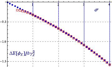
σ\sigma Δ​E​[ϕK(σ)]\Delta E[\phi_{\rm K}^{(\sigma)}] 0.0{\bf 0.0} 0.000000.00000 0.010.01 −0.0040164-0.0040164 0.10.1 −0.037024-0.037024 0.20.2 −0.070414-0.070414 0.30.3 −0.102158-0.102158 0.40.4 −0.133080-0.133080 0.50.5 −0.163637-0.163637 0.60.6 −0.194114-0.194114 0.70.7 −0.224700-0.224700 0.80.8 −0.255533-0.255533 0.90.9 −0.286711-0.286711 0.990.99 −0.315129-0.315129   σ\sigma Δ​E​[ϕK(σ)]\Delta E[\phi_{\rm K}^{(\sigma)}] 1.0{\bf 1.0} −0.31831-0.31831 1.011.01 −0.321495-0.321495 1.11.1 −0.350388-0.350388 1.21.2 −0.382994-0.382994 1.31.3 −0.416163-0.416163 1.41.4 −0.449927-0.449927 1.51.5 −0.484311-0.484311 1.61.6 −0.519340-0.519340 1.71.7 −0.555028-0.555028 1.81.8 −0.591393-0.591393 1.91.9 −0.628449-0.628449 1.991.99 −0.662399-0.662399   σ\sigma Δ​E​[ϕK(σ)]\Delta E[\phi_{\rm K}^{(\sigma)}] 2.0{\bf 2.0} −0.666254-0.666254 2.012.01 −0.670018-0.670018 2.12.1 −0.704683-0.704683 2.22.2 −0.743871-0.743871 2.32.3 −0.783797-0.783797 2.42.4 −0.824449-0.824449 2.52.5 −0.865861-0.865861 2.62.6 −0.908014-0.908014 2.72.7 −0.950919-0.950919 2.82.8 −0.986907-0.986907 2.92.9 −1.03902-1.03902 2.992.99 −1.07967-1.07967   σ\sigma Δ​E​[ϕK(σ)]\Delta E[\phi_{\rm K}^{(\sigma)}] 3.0{\bf 3.0} −1.08451-1.08451 3.013.01 −1.08878-1.08878 3.13.1 −1.13019-1.13019 3.23.2 −1.17694-1.17694 3.33.3 −1.22446-1.22446 3.43.4 −1.27276-1.27276 3.53.5 −1.32184-1.32184 3.63.6 −1.37171-1.37171 3.73.7 −1.42237-1.42237 3.83.8 −1.47381-1.47381 3.93.9 −1.52605-1.52605 3.993.99 −1.57374-1.57374

Table 4: One-loop parent kink mass shifts for several values of σ∈[0.0,4.0]\sigma\in[0.0,4.0] estimated by applying the generalized DHN formula.

Refer to caption      Refer to caption

Figure 4: Graphical representation of: (a) one-loop kink mass shifts in the range: σ∈[0.0,4.0]\sigma\in[0.0,4.0]. (b) Seeley coefficients within the same range.

The values depicted in Table 4 have been drawn in Figure 4 as solid points. The figure shows a remarkable pattern: the continuity of Δ​E​[ϕK(σ)]\Delta E[\phi_{\rm K}^{(\sigma)}] as a function of the parameter σ\sigma. The generalized DHN formula (derived in the mode-number cut-off regularization procedure plus a 12\frac{1}{2}-weight on the half-bound states coming from the 1D Levinson theorem) guarantees this behaviour. Had we applied the original DHN formula for all values of σ∈ℝ\sigma\in\mathbb{R} we would have found discontinuities at integers values of σ\sigma. Note also that Δ​E​[ϕK(σ)]/md​ℏ\Delta E[\phi_{\rm K}^{(\sigma)}]/m_{d}\hbar tends to zero when σ\sigma vanishes, as should be the case, see Figure 4(a).

3.2.2 The asymptotic approach

Finally, we shall apply the asymptotic approach in the σ∉ℕ\sigma\notin\mathbb{N} models. In this case, computation of the Seeley coefficients cn​(K(σ))c_{n}(K^{(\sigma)}) in (36) can only be achieved by solving the recurrence relations (40). In Reference [21] a symbolic program code has been developed that performs this laborious task. We use this code to calculate the Seeley coefficients, adapted to the present models. A graphical representation of these coefficients is shown in Figure 4(b) for different values of the σ\sigma parameter with a separation of 0.1 in the range [0.4,2.0][0.4,2.0]. In general, the larger the value of σ\sigma, the larger the coefficients cn​(K(σ))c_{n}(K^{(\sigma)}). Plugging these coefficients into formula (36) we estimate the quantum correction. Frequently, the response of (36) has been evaluated by employing a series involving ten terms, i.e., Nt=10N_{t}=10, although this can vary along the values of the parameter σ\sigma. The results obtained are shown in Table 5.

σ\sigma Δ​E​[ϕK(σ)]\Delta E[\phi_{\rm K}^{(\sigma)}] 0.0{\bf 0.0} −⁣−-- 0.010.01 −⁣−-- 0.10.1 −⁣−-- 0.20.2 −⁣−-- 0.30.3 −⁣−-- 0.40.4 −0.201364-0.201364 0.50.5 −0.211213-0.211213 0.60.6 −0.224572-0.224572 0.70.7 −0.241903-0.241903 0.80.8 −0.263464-0.263464 0.90.9 −0.289269-0.289269 0.990.99 −0.316476-0.316476   σ\sigma Δ​E​[ϕK(σ)]\Delta E[\phi_{\rm K}^{(\sigma)}] 1.0{\bf 1.0} −0.318321-0.318321 1.011.01 −0.322882-0.322882 1.11.1 −0.352179-0.352179 1.21.2 −0.385393-0.385393 1.31.3 −0.416517-0.416517 1.41.4 −0.450447-0.450447 1.51.5 −0.484716-0.484716 1.61.6 −0.519600-0.519600 1.71.7 −0.555152-0.555152 1.81.8 −0.591376-0.591376 1.91.9 −0.628289-0.628289 1.991.99 −0.662103-0.662103   σ\sigma Δ​E​[ϕK(σ)]\Delta E[\phi_{\rm K}^{(\sigma)}] 2.0{\bf 2.0} −0.666241-0.666241 2.012.01 −0.669769-0.669769 2.12.1 −0.704338-0.704338 2.22.2 −0.743427-0.743427 2.32.3 −0.783236-0.783236 2.42.4 −0.823772-0.823772 2.52.5 −0.865044-0.865044 2.62.6 −0.907056-0.907056 2.72.7 −0.949812-0.949812 2.82.8 −0.99332-0.99332 2.92.9 −1.03758-1.03758 2.992.99 −1.07807-1.07807   σ\sigma Δ​E​[ϕK(σ)]\Delta E[\phi_{\rm K}^{(\sigma)}] 3.0{\bf 3.0} −1.08441-1.08441 3.013.01 −1.08714-1.08714 3.13.1 −1.12839-1.12839 3.23.2 −1.17493-1.17493 3.33.3 −1.22225-1.22225 3.43.4 −1.27033-1.27033 3.53.5 −1.31919-1.31919 3.63.6 −1.36882-1.36882 3.73.7 −1.41924-1.41924 3.83.8 −1.47043-1.47043 3.93.9 −1.52240-1.52240 3.993.99 −1.56984-1.56984

Table 5: One-loop (15) kink mass shifts for several values of σ∈[0.0,4.0]\sigma\in[0.0,4.0] estimated by applying the asymptotic approach.

The values seen in the Table 5 are drawn in Figure 4(a) as empty squares in order to appreciate the concordance between the data obtained upon using the generalized DHN formula and the asymptotic approach. Only a small difference between the data arises for σ≤0.6\sigma\leq 0.6 and lower. For σ\sigma small the series in (36) converges slowly because of the factor (σ2)1−n(\sigma^{2})^{1-n} in each summand; a larger number of terms is needed to obtain a precise answer. The limitations in the computations of the Seeley coefficients make the asymptotic approach less exact in the range of values of the parameter σ<0.4\sigma<0.4.

4 Conclusions and further comments

We have constructed a one-parametric family of (1+1)-dimensional one-component scalar field theory models governed by the action (2) with the potential (18). This family includes two famous members: the sine-Gordon and ϕ4\phi^{4} models. The models in this family are characterized by very specific kink wells: the second-order kink fluctuation operators are Schrödinger operators with Pöschl-Teller potential wells. In general, the family of potentials (18) is only of 𝒞2​(ℝ){\cal C}^{2}(\mathbb{R}) class as a function of the field ϕ\phi: Derivatives of order higher than two are discontinuous or divergent at the vacuum points. There exists a similar family of models, with class 𝒞∞{\cal C}^{\infty} potentials, for two or more scalar fields. For example, the (1+1)-dimensional two-component scalar field theory model with a 𝒞∞​(ℝ2){\cal C}^{\infty}(\mathbb{R}^{2}) potential

U⁡(ϕ1,ϕ2)=18​(4​ϕ12+2​σ​ϕ22−1)2+2​σ2​ϕ12​ϕ22U(\phi_{1},\phi_{2})=\frac{1}{8}(4\phi_{1}^{2}+2\sigma\phi_{2}^{2}-1)^{2}+2\sigma^{2}\phi_{1}^{2}\phi_{2}^{2}

admits the kink solution

ϕ1K​(x)=12​tanh⁡x¯,ϕ2K​(x)=0\phi_{1}^{\rm K}(x)=\frac{1}{2}\tanh\overline{x}\hskip 28.45274pt,\hskip 28.45274pt\phi_{2}^{\rm K}(x)=0

whose second-order small fluctuation operator is:

K(σ)=(−d2d​x2+4−6​sech2​x¯00−d2d​x2+σ2−σ⁡(σ+1)​sech2​x¯).K^{(\sigma)}=\left(\begin{array}[]{cc}-\frac{d^{2}}{dx^{2}}+4-6\,{\rm sech}^{2}\,\overline{x}&0\\ 0&-\frac{d^{2}}{dx^{2}}+\sigma^{2}-\sigma(\sigma+1)\,{\rm sech}^{2}\,\overline{x}\end{array}\right)\qquad.

Here, the generic Pöschl-Teller potential well arises in the study of the orthogonal fluctuations to the kink solution, see [9].

Finally, the spectral problems associated with kink stability analysis in the models studied in this paper are solvable and therefore the one-loop quantum correction to the kink mass in these cases can be computed exactly. By the same token as before, Δ​E⊥​[ϕK(σ)]\Delta E^{\bot}[\phi_{\rm K}^{(\sigma)}], the one-loop kink mass shift due to orthogonal fluctuations to the kink, is a continuous function of σ\sigma. Note, however, that our methods have been improved such that the agreement between the results via the generalized DHN formula and the asymptotic method is now much better than eight years ago, see [9].

ACKNOWLEDGEMENTS

We gratefully acknowledge partial funding from the Spanish Ministerio de Educacion y Ciencia (DGICYT) under grant: FIS2009-10546.

References

  • [2] N.H. Christ, T.D. Lee, Quantum expansions of soliton solutions, Phys. Rev. D12 no. 6 (1975) 1606-1627.
  • [3] S.E. Trullinger, R.J. Flesch, Parent potentials for an infinite class of reflectionless kinks, J. Math. Phys. 28 (8) (1987) 1683-1690.
  • [4] Cahill, K.; Comtet, A.; Glauber, R.; “Mass formulas for static solitons”, Phys. Lett. 64B (1976) 283-385.
  • [5] L.J. Boya, J. Casahorran, General scalar bidimensional models including kinks, Annals of Physics, 196 (1989) 361-385.
  • [6] R. Dashen, B. Hasslacher and A. Neveu, “Non-perturbative methods and extended hadron models in field theory: 1. semiclassical functional methods; 2. two-dimensional models and extended hadrons; 3. four dimensional non-Abelian models”, Phys. Rev. D10 (1974) 4114-4130.
  • [7] R. Dashen, B. Hasslacher and A. Neveu, Phys. Rev. D11 (1975) 3424.
  • [8] R. Dashen, B. Hasslacher and A. Neveu, Phys. Rev. D12 (1975) 2443.
  • [9] A. Alonso-Izquierdo, J.M. Guilarte, M.A.G. Leon, W. G. Fuertes, One-loop corrections to classical masses of kink families, Nucl. Phys. B 681 (2004) 163-194.
  • [10] A. Rebhan and P. van Nieuwenhuizen, “No saturation of the quantum Bogomolny bound by two-dimensional 𝒩=1{\cal N}=1 solitons”, Nucl. Phys. B508 (1997) 449-467.
  • [11] H. Nastase, M. Stephanov, A. Rebhan and P. van Nieuwenhuizen, “Topological boundary conditions, the BPS bound and elimination of ambiguities in quantum mass of solitons”, Nucl. Phys. B542 (1999) 471.
  • [12] Goldhaber, A.; Rebhan, A.; van Nieuwenhuizen, P.; Wimmer, R.;, “Quantum corrections to mass and central charge of sypersymmetric solitons”, Phys. Rept. 𝟑𝟗𝟖​𝐂{\bf 398C} (2004) 179, [arXiv:hep-th/0401152].
  • [13] Rebhan, A.; van Nieuwenhuizen, P.; Wimmer, R.;, “New developments in the quantization of sypersymmetric solitons (kinks, vortices and monopoles)”, Braz. J. Phys. 𝟑𝟒{\bf 34} (2004) 1273-1287, [arXiv:hep-th/0404223].
  • [14] M. Shifman, A. Vainshtein and M. Voloshin, “Anomaly and quantum corrections to solitons in two-dimensional theories with minimal supersymmetry ”, Phys. Rev. D59(1999) 045016.
  • [15] N. Graham and R. Jaffe, “Energy, central charge, and the BPS bound for 1+1 dimensional supersymmetric solitons”, Nucl. Phys. 𝐁𝟓𝟒𝟒{\bf B544} (1999) 432-447.
  • [16] N. Graham and R. Jaffe, “Fermionic one-loop corrections to soliton energies in 1+1 dimensions”, Nucl. Phys. 𝐁𝟓𝟒𝟗{\bf B549} (1999) 516-526.
  • [17] M. Bordag, “Vacuum energy in smooth background fields”, J. Phys. A28 (1995) 755
  • [18] M. Bordag, A. Goldhaber, P. van Nieuwenhuizen and D. Vassilevich, Heat kernels and zeta-function regularization for the mass of the SUSY kink, Phys. Rev. D66 (2002) 125014.
  • [19] Mateos Guilarte, J; Alonso-Izquierdo, A.; García Fuertes, W.; de la Torre Mayado, M.; Senosiaín, M. J.; Quantum fluctuations around low-dimensional topological defects, Proceedings of Science (ISFTG) 013 (2009) (63pp).
  • [20] A. Alonso-Izquierdo, J.M. Guilarte, M.A.G. Leon, W. G. Fuertes, Generalized zeta functions and one-loop corrections to quantum kink masses, Nucl. Phys. B 635 (2002) 525-557
  • [21] A. Alonso-Izquierdo, J. Mateos Guilarte.; One-loop kink mass shifts: a computational approach, Nuclear Physics B852 (2011) 696-735.
  • [22] Drazin, P. G. and Johnson; R. S., “Solitons: an introduction”, Cambridge University Press, Cambridge U. K., 1989
  • [23] V. E. Zakharov and L. D. Faddeev, Functional Analysis Applic. 5 (1972)280
  • [24] Gilkey, P.B., “Invariance theory, the Heat equation and the Atiyah-Singer index theorem”, Publish or Perish, Inc 1984.
  • [25] Roe, J.; Elliptic operators, topology and asymptotic methods Longman Scientific and Technical, New York (1988).
  • [26] Vassilevich, D.V.; “Heat kernel expansion: user’s manual”, Phys. Rep. 𝟑𝟖𝟖​𝐂{\bf 388C} (2003) 279-360.
  • [27] Rajaraman, R.; “Solitons and instantons”, North Holland, Amsterdam, 1982.
  • [28] A. Alonso-Izquierdo, W. García Fuertes, M. A. González León, M. de la Torre Mayado, J. Mateos Guilarte, J. M. Muñoz-Castañeda, “Lectures on the mass of topological solitons”, arXiv: [hep-th/0611180] (99pp).
  • [29] de Witt, B.S.; “Dynamical theory of groups and fields”, Gordon and Breach, 1965.
  • [30] Avramidi, I. G.; “Heat kernel approach in quantum field theory”, Nucl. Phys. Proc. Sup. 104(2002)3-32, [arXiv;hep-th/0107018]
  • [31] A. Alonso-Izquierdo, J.M. Guilarte, M.A.G. Leon, W. G. Fuertes, Semi-classical mass of of quantum k-component topological kinks, Nucl. Phys. B 638 (2002) 378
  • [32] A. Alonso-Izquierdo, W. G. Fuertes, M. de la Torre, J.M. Guilarte, Quantum oscillations of self-dual Abrikosov-Nielsen-Olesen vortices, Phys. Rev. D71 (2005) 125010.
  • [33] A. Alonso-Izquierdo, W. G. Fuertes, M. de la Torre, J.M. Guilarte, One-loop fluctuations of semi-local self-dual vortices, J. Phys. A, 41 (2008) 164050.