Intensity distribution of non-linear scattering states

Timo Hartmann Affiliation: Institut für Theoretische Physik, Universität Regensburg, 93040 Regensburg, Germany Juan-Diego Urbina Affiliation: Institut für Theoretische Physik, Universität Regensburg, 93040 Regensburg, Germany Klaus Richter Affiliation: Institut für Theoretische Physik, Universität Regensburg, 93040 Regensburg, Germany Peter Schlagheck Affiliation: Département de Physique, Université de Liège, 4000 Liège, Belgium

Abstract

We investigate the interplay between coherent effects characteristic of the propagation of linear waves, the non-linear effects due to interactions, and the quantum manifestations of classical chaos due to geometrical confinement, as they arise in the context of the transport of Bose-Einstein condensates. We specifically show that, extending standard methods for non-interacting systems, the body of the statistical distribution of intensities for scattering states solving the Gross-Pitaevskii equation is very well described by a local Gaussian ansatz with a position-dependent variance. We propose a semiclassical approach based on interfering classical paths to fix the single parameter describing the universal deviations from a global Gaussian distribution. Being tail effects, rare events like rogue waves characteristic of non-linear field equations do not affect our results.

I Introduction

The progress on the experimental preparation and manipulation of interacting Bose-Einstein condensates has given a strong boost to the study of non-linear wave equations that account for the effect of interactions within the condensate in the framework of a mean-field approximation. Particularly promising cold-atom experiments in the context of transport physics include the realization of guided atom lasers [1, 2, 3, 4], of arbitrarily shaped confinement potentials for cold atoms [6, 7, 5], as well as of artificial gauge fields that break the time-reversal invariance for neutral atoms [8, 9]. This makes it now feasible to experimentally explore the coherent transport of Bose-Einstein condensates through various mesoscopic structures that can possibly be modeled by billiard configurations.

An interesting question that rises in this context is how the presence of the atom-atom interaction within the coherent matter waves affects interference effects well that are established for non-interacting systems. Indeed, previous theoretical studies have focused on the question how coherent backscattering in disordered potentials is modified by the presence of the atom-atom interaction [10]. These studies were recently complemented by our investigations on weak localization in the nonlinear transport through ballistic scattering geometries that exhibit chaotic dynamics [11]. While a semiclassical analysis of this nonlinear scattering problem predicted a dephasing of the interference phenomenon that gives rise to coherent backscattering, signatures for weak antilocalization were obtained in the numerically computed reflection and transmission probabilities [11]. This effect was attributed to the specific role of non-universal short-path contributions, in particular to self-retraced paths the presence of which gives rise to a reduction of coherent backscattering as compared to the universal prediction.

In the present work, we consider the same scenario as in Ref. [11], i.e., the quasi-stationary transport of bosonic matter waves through two-dimensional ballistic scattering geometries that exhibit chaotic classical dynamics. In contrast to Ref. [11], however, we focus here not on transport observables such as the reflection and transmission probabilities through the billiard, but rather on the intensity distributions of stationary scattering states within the billiard. These intensity distributions are to be compared with the theoretical predictions that are obtained from the Random Wave Model (RWM) [12, 13, 14, 15], which, in the linear case, represents probably the most powerful approach to describe the universal spatial correlations of eigenstates arising from the classical chaotic behavior due to the presence of a spatial confinement. A most natural question that arises here is then to which extent the basic assumptions behind this model can also be used to describe possible universal spatial fluctuations in collective coherent matter waves that exhibit a weak atom-atom interaction. Within a mean-field semiclassical description, such matter waves are well described by the Gross-Pitaevskii equation [16] in which the presence of interaction is accounted for by means of a non-linear interaction potential. This equation is the starting point of our calculations, both on the numerical and on the analytical side.

It is important to mention that rare effects due to the nonlinearity of the wave equation like rogue waves [17] or due to the presence of disorder, like branching [18], will certainly affect the tails of the intensity distribution, and such effects are in principle outside the reach of our approach. Therefore, we will rstrict ourselves to the body of the distribution, where rare events need not to be considered.

The paper is organized as follows. We describe in Section II the scattering configuration under consideration as well as the main observable to be discussed in this work. In Section III, we present a semiclassical theory of the intensity distribution in this nonlinear system, which is based on the Gaussian hypothesis as well as on the semiclassical theory of coherent backscattering in nonlinear systems. The predictions obtained by this semiclassical theory will be compared with the numerical results at the end of Section III, followed by a discussion in Section IV.

II Stationary scattering states of the Gross-Pitaevskii equation

For our simulations, we use the inhomogeneous two-dimensional Gross-Pitaevskii equation

i\hbar\frac{\partial}{\partial t}\Psi(\mathbf{\boldsymbol{r}},t)=H\Psi(\mathbf{\boldsymbol{r}},t)+g(\mathbf{\boldsymbol{r}})\frac{\hbar^{2}}{m}|\Psi(\mathbf{\boldsymbol{r}},t)|^{2}\Psi(\mathbf{\boldsymbol{r}},t)+S(\mathbf{\boldsymbol{r}})e^{-it\mu/\hbar}

(1)

where we have introduced the single particle Hamiltonian

H=\frac{1}{2m}\left[-i\hbar\mathbf{\boldsymbol{\nabla}}-q\mathbf{\boldsymbol{A}}(\mathbf{\boldsymbol{r}})\right]^{2}+V(\mathbf{\boldsymbol{r}})

(2)

with the billiard potential $V(\mathbf{\boldsymbol{r}})$ . This Gross-Pitaevskii equation contains a source term

S(\mathbf{r})=S_{0}\chi_{i}(y)\delta(x-x_{L})\;

(3)

which models the injection of atoms in a Bose-Einstein condensate acting as a reservoir with the chemical potential $\mu$ into the scattering system [19]. $\chi_{i}(y)$ is a transverse eigenmode of the incident lead and $S_{0}$ controls the current that is injected into the billiard.

The non-linear potential term $g(\mathbf{\boldsymbol{r}})\frac{\hbar^{2}}{m}|\Psi(\mathbf{\boldsymbol{r}},t)|^{2}\Psi(\mathbf{\boldsymbol{r}},t)$ describes atom-atom scattering events. Assuming that the degree of motion for the third spatial dimension is frozen out, e.g. by applying a harmonic confinement potential in this direction, we obtain the effective two-dimensional interaction strength as $g(\mathbf{r})={2}\sqrt{2\pi}a_{s}/\sqrt{\hbar/[m\omega_{\perp}(\mathbf{r})]}$ where $a_{s}$ is the s-wave scattering length of the atomic species under consideration and $\omega_{\perp}$ is the confinement frequency in the third spatial dimension. A spatial variation $\omega_{\perp}\equiv\omega_{\perp}(\mathbf{r})$ of this confinement will then naturally induce a corresponding variation in $g\equiv g(\mathbf{r})$ . We shall, in the following, consider an effective interaction strength $g(\mathbf{r})$ that is homogeneous within the billiard and vanishes in the attached leads. In a similar manner, we shall also assume that the artificial gauge field is given by $\mathbf{A}(\mathbf{r})=\frac{1}{2}B\mathbf{e}_{\perp}\times\mathbf{r}$ (with $\mathbf{e}_{\perp}$ the unit vector in the third spatial dimension), with an effective “magnetic field” strength $B$ that is constant within the billiard and vanishes in the leads.

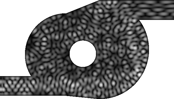
The billiard geometry considered in this work is shown in Fig. 1. It is characterized by the billiard area $\Omega$ and the typical energy $E_{0}$ of the incident matter-wave beam. Using these quantities, we can define a time scale $\hbar/E_{0}$ , a length scale $k_{0}^{-1}$ with $E_{0}\equiv\hbar^{2}k^{2}_{0}/(2m)$ , and a scale $B_{0}\equiv 2\pi\hbar/(q\Omega)$ (the flux quantum) for the magnetic field. All quantities in this work will be measured in these units. The area of the system is determined as $k_{0}\Omega^{1/2}=81.2$ . Two leads are attached to the billiard, which transforms it into an open scattering system. The width of the leads is given by $W=5.4\,\pi/k_{0}$ , which means that five channels are open in each of the leads.

Refer to caption — Figure 1: The shape of the billiard used in this work together with the density of a typical stationary scattering state. The hatched area in the left figure marks the region used for calculating the intensity distribution (adapted from Ref. [11]).

In order to calculate the stationary scattering states within this configuration, we insert the ansatz

\Psi(\mathbf{\boldsymbol{r}},t)=\Psi(\mathbf{\boldsymbol{r}})e^{-it\mu/\hbar}

(4)

into Eq. (1). This yields the self-consistent non-linear equation

\left[\mu-H-g(\mathbf{\boldsymbol{r}})\frac{\hbar^{2}}{m}|\Psi(\mathbf{\boldsymbol{r}})|^{2}\right]\Psi(\mathbf{\boldsymbol{r}})=S(\mathbf{\boldsymbol{r}})

(5)

for the stationary scattering state. The amplitude of the source term is fixed such that in incident current of $j_{in}=1\,E_{0}/\hbar$ is generated. Varying $j_{in}$ provides yet another way to effectively change the interaction strength $g$ , as Eq. (5) is invariant under the scaling $(g,j_{in},\Psi)\mapsto(g\,\eta^{-2},j_{in}\,\eta^{2},\Psi\,\eta)$ (for $\eta\in\mathbb{R}$ ).

The non-linear scattering problem Eq. (5) is now solved using the methods described in Appendix A. We performed computations for 50 different values of the energy $\mu$ (all in the energy range $0.93\,E_{0}\dots 1.18\,E_{0}$ where five lead channels are open), for 25 different positions of the spherical obstacle in the centre of the billiard, and for the five different lead channels. The thereby obtained stationary scattering states $\Psi(\mathbf{\boldsymbol{r}})$ are now used to determine the intensity distribution, i.e. the probability distribution of $|\Psi(\mathbf{\boldsymbol{r}})|^{2}$ , and its mean value. Only the points inside the marked region in Fig. 1 were used. Points in the vicinity of a boundary have to be avoided as explained in Sec. III.

The left panel of Fig. 2 shows the probability distribution for obtaining a given real part of the scattering wavefunction (which is the same as for the imaginary part) within the marked region of the billiard in the linear ( $g=0$ ) and time-reversal invariant ( $B=0$ ) case. We find a very good agreement with a Gaussian distribution. Consequently, the intensity $I\equiv|\Psi|^{2}/\langle|\Psi|^{2}\rangle$ is distributed according to a Porter-Thomas law $P(I)\simeq e^{-I}$ , as is confirmed in the right panel of Fig. 2. There are tiny but systematic deviations from the Porter-Thomas law which slightly underestimates the actual intensity distribution near $I=0$ (as is also seen in the left panel of Fig. 2) as well as for very large intensities $I\gtrsim 5$ , and overestimates it in between for $1\lesssim I\lesssim 3$ .

To highlight these deviations, we plot in Fig. 3 $P(I)e^{I}$ as a function of the intensity $I$ , for various values of the nonlinearity $g$ and the magnetic field strength $B$ . A parabolic behaviour with a minimum at $I=2$ is found. The prefactor of this parabolic scaling is reduced with increasing $g$ . This appears natural as a weak repulsive interaction between the atoms is generally expected to give rise to a flattening of the density distribution, leading, in particular, to a significant reduction of intensity maxima, in order to minimize the interaction energy within the condensate (see also Ref. [20] for an analogous phenomenology in nonlinear optics in the presence of a defocusing nonlinearity). Indeed, similar findings were obtained for the quasi-stationary transport of Bose-Einstein condensates through two-dimensional disorder potentials [21], for which is was found that the parabolic scaling of $P(I)e^{I}$ with the intensity $I$ could even become inverted at stronger nonlinearities $g$ . The dependence of the parabolic scaling with the magnetic field $B$ , on the other hand, is related to coherent backscattering, for which we shall develop a semiclassical theory in the following section.

Figure 2: Left panel: numerical probability distribution (dots) of the real part of the wavefunction for

B=0

and

g=0

, which agrees very well with a Gaussian distribution (solid line). The same holds for the imaginary part. The right panel compares the numerically obtained intensity distributions

P_{g}(I)

for

g=0

and

g=0.05

(

B=0

in both cases) with the Porter-Thomas distribution

e^{-I}

. Note the tiny but systematic deviations from the Porter-Thomas law, which are highlighted in Fig. 3.

Figure 3: Deviation of the intensity distributions from the Poster-Thomas law for several values of the interaction strength

g

(left panel, with

B=0

) and of the magnetic field

B

in units of

B_{0}

(right panel, for

g=0

)

III The semiclassical approach to the intensity distribution

In a first step, and following the now standard approach to describe the statistical properties of eigenfunctions in non-interacting and classically chaotic billiard systems [12], we shall make the fundamental assumption that scattering eigenstates of the non-linear Schrödinger equation share the same correlations as an ensemble of Gaussian Random Fields (see the left panel of Fig. 2). This assumption leads to a Poster-Thomas distribution $P(I)=e^{-I}$ for the normalized intensity $I=|\Psi|^{2}/\left\langle|\Psi|^{2}\right\rangle$ (see Eq. (7) below) which, as discussed above, is supported by our numerical findings, as seen in the right panel of Fig. 2. The presence of a weak interaction does not change the excellent agreement of the numerical data with a Porter-Thomas profile.

Knowing that the general features of the distribution of intensities for nonlinear waves are well described by a Porter-Thomas distribution, we now ask whether the deviations observed in Fig. 3 have also such universal character. Once again, the guiding principle will be linear case, where deviations from the body of the distribution are consistent with a Gaussian random field with a variance that smoothly depends on the local position. This consideration leads to an universal form of the deviations given by a Laguerre polynomial, which therefore depend only on a single parameter [13]. Fig. 3 shows how this property of the non-interacting case takes over perfectly when interactions are present.

The final step will be the explicit calculation of the coefficient in front of the polynomial corrections, and in particular its dependence on the strength of the interaction and of the magnetic field. Here we shall assume that a basic property of scattering states in the linear case, namely that their average intensity over energy and channels is related with the imaginary part of the full Green function, holds approximately in the presence of interactions as well. Assuming ergodicity within the billiard and utilizing the semiclassical approach presented in Ref. [11], we obtain an explicit expression for the variation of the polynomial prefactor with the magnetic field strength for various values of the nonlinearity.

III.1 The local Gaussian approach

The calculation of the intensity distribution uses the values of $|\Psi(\mathbf{\boldsymbol{r}})|^{2}$ at many different positions, incoming channels, and energies. Thus, both an energy and a position average is involved. Motivated by the idea that for fixed position $\mathbf{\boldsymbol{r}}$ , the average intensity over energy and channels $\left\langle\left|\Psi(\mathbf{\boldsymbol{r}})\right|^{2}\right\rangle_{E}$ is itself a smooth function of $\mathbf{\boldsymbol{r}}$ , the double averaging procedure is now split apart.

We start therefore by assuming a position-dependent Gaussian distribution

{P_{\mathbf{\boldsymbol{r}}}\left(\Psi_{r},\Psi_{i}\right)=\frac{1}{\pi\left\langle\left|\Psi(\mathbf{\boldsymbol{r}})\right|^{2}\right\rangle_{E}}\exp\left[-\frac{\Psi_{r}^{2}+\Psi_{i}^{2}}{\left\langle\left|\Psi(\mathbf{\boldsymbol{r}})\right|^{2}\right\rangle_{E}}\right]}

(6)

for the real and the imaginary part of the wave function ( $\Psi{\equiv}\Psi_{r}+i\Psi_{i}$ ) at a fixed point $\mathbf{\boldsymbol{r}}$ , where $\left\langle\left|\Psi(\mathbf{\boldsymbol{r}})\right|^{2}\right\rangle_{E}$ denotes the energy and channel average of the intensity. For non-interacting systems with chaotic classical dynamics, such a local Gaussian distribution is a rigorous consequence of the Random Wave Model [22], and the possible universality of the deviations from the fully homogeneous case, i.e. from the case that $\left\langle\left|\Psi(\mathbf{\boldsymbol{r}})\right|^{2}\right\rangle_{E}$ is independent of the position $\mathbf{\boldsymbol{r}}$ , are encoded in $\left\langle\left|\Psi(\mathbf{\boldsymbol{r}})\right|^{2}\right\rangle_{E}$ (see Ref. [13]). At a boundary the wavefunction vanishes and thus $\left\langle\left|\Psi(\mathbf{\boldsymbol{r}})\right|^{2}\right\rangle_{E}$ vanishes there, too. Such boundary effects can also be incorporated in our approach. In this work, however, we shall restrict our study to the bulk, and therefore points in the vicinity of a boundary will be avoided. The distribution for the intensity ${\rho\equiv}\left|\Psi\right|^{2}$ is now calculated as

	$\displaystyle P_{\mathbf{\boldsymbol{r}}}({\rho})$	$\displaystyle=$	$\displaystyle\int_{-\infty}^{+\infty}{\int_{-\infty}^{+\infty}}P_{\mathbf{\boldsymbol{r}}}(\Psi_{r},\Psi_{i})\;\delta({\rho}-{\Psi_{r}^{2}-\Psi_{i}^{2}})\;d\Psi_{r}d\Psi_{i}$		(7)
		$\displaystyle=$	$\displaystyle\frac{1}{\left\langle\left\|\Psi(\mathbf{\boldsymbol{r}})\right\|^{2}\right\rangle_{E}}\exp\left[-\frac{{\rho}}{\left\langle\left\|\Psi(\mathbf{\boldsymbol{r}})\right\|^{2}\right\rangle_{E}}\right]\,{,}$		(7)

which is a local Porter-Thomas distribution for ${\rho}$ .

Figure 4: Comparison of the numerically obtained intensity distributions with Eq. (10). The unknown parameter

\beta

is determined by fitting Eq. (10) (shown as dashed lines and marker symbols) to the numerical data (solid lines). The fitting is done in the range

1\leq I\leq 7

We now proceed by splitting $\left\langle\left|\Psi(\mathbf{\boldsymbol{r}})\right|^{2}\right\rangle_{E}$ into a position-dependent part and a position-independent part

\left\langle\left|\Psi(\mathbf{\boldsymbol{r}})\right|^{2}\right\rangle_{E}=\frac{1}{A}\left[1+C(\mathbf{\boldsymbol{r}})\right]

(8)

by imposing the condition that the position average of $C(\mathbf{\boldsymbol{r}})$ is zero: $\left\langle C(\mathbf{\boldsymbol{r}})\right\rangle_{\mathbf{\boldsymbol{r}}}=0$ . Using $\left\langle 1\right\rangle_{\mathbf{\boldsymbol{r}}}=1$ , we obtain relation $\left\langle\left\langle\left|\Psi(\mathbf{\boldsymbol{r}})\right|^{2}\right\rangle_{E}\right\rangle_{\mathbf{\boldsymbol{r}}}=A^{-1}=\left\langle|\Psi(\mathbf{\boldsymbol{r}})|^{2}\right\rangle$ . Introducing the normalized intensity $I=A{\rho}$ , we can now rewrite the intensity distribution as

	$\displaystyle P_{\mathbf{\boldsymbol{r}}}(I)$	$\displaystyle=$	$\displaystyle\frac{1}{1+C(\mathbf{\boldsymbol{r}})}\exp\left[-\frac{I}{1+C(\mathbf{\boldsymbol{r}})}\right]=\frac{e^{-I}}{1-(-C(\mathbf{\boldsymbol{r}}))}\exp\left[-\frac{I\;(-C(\mathbf{\boldsymbol{r}}))}{(-C(\mathbf{\boldsymbol{r}}))-1}\right]$		(9)
		$\displaystyle=$	$\displaystyle e^{-I}\;\sum_{n=0}^{\infty}(-1)^{n}\left[C(\mathbf{\boldsymbol{r}})\right]^{n}L_{n}(I)$		(9)

where in the last step we use the generating function of the Laguerre polynomials $L_{n}(I)$ [23]. Finally, we perform a position average to obtain, up to second order in $I$ , the normalized intensity distribution

	$\displaystyle P(I){\equiv}\left\langle P_{\mathbf{\boldsymbol{r}}}(I)\right\rangle_{\mathbf{\boldsymbol{r}}}$	$\displaystyle=$	$\displaystyle e^{-I}\left[1+\left\langle C(\mathbf{\boldsymbol{r}})^{2}\right\rangle_{\mathbf{\boldsymbol{r}}}L_{2}(I)\right]$		(10)
		$\displaystyle{=}$	$\displaystyle{e^{-I}\left[1+\beta\left(1-2I+\frac{1}{2}I^{2}\right)\right]}$		(10)

with $\beta\equiv\left\langle C(\mathbf{\boldsymbol{r}})^{2}\right\rangle_{\mathbf{\boldsymbol{r}}}$ . In Fig. 4 we compare this formula with the numerically obtained intensity distributions. We see that the numerical data are very well described by a behaviour of the form (10), with $\beta$ being the only free parameter. This supports our claim that for weak interactions, deviations of the intensity distribution are universal and depend only on a single parameter.

III.2 Semiclassical calculation of $\beta$

The parameter $\beta$ can be numerically obtained by a fitting procedure and compared with a prediction based on the semiclassical approximation to the non-linear Green function $G(\mathbf{\boldsymbol{r}},\mathbf{\boldsymbol{r}}^{\prime},E)$ defined through

\left[E-H-g(\mathbf{\boldsymbol{r}})\frac{\hbar^{2}}{m}|G(\mathbf{\boldsymbol{r}},\mathbf{\boldsymbol{r}}^{\prime},E)|^{2}\right]G(\mathbf{\boldsymbol{r}},\mathbf{\boldsymbol{r}}^{\prime},E)=\delta(\mathbf{\boldsymbol{r}}-\mathbf{\boldsymbol{r}}^{\prime})\;.

(11)

In order to understand the connection between the parameter $\beta$ and the nonlinear Green function, we consider first the Green function $G_{0}$ for the linear system,

\left[E-H\right]G_{0}(\mathbf{\boldsymbol{r}},\mathbf{\boldsymbol{r}}^{\prime},E)=\delta(\mathbf{\boldsymbol{r}}-\mathbf{\boldsymbol{r}}^{\prime}),

(12)

which admits a spectral decomposition in terms of the normalized scattering states $\Psi_{E^{\prime},\alpha}(\mathbf{\boldsymbol{r}})$ at energy $E^{\prime}$ with incoming channel $\alpha$ , given by

G^{\pm}_{0}(\mathbf{\boldsymbol{r}},\mathbf{\boldsymbol{r}}^{\prime},E)=\sum_{\alpha}\int dE^{\prime}\frac{\Psi_{E^{\prime},\alpha}(\mathbf{\boldsymbol{r}})\Psi_{E^{\prime},\alpha}(\mathbf{\boldsymbol{r}}^{\prime})^{*}}{E-E^{\prime}\pm i0^{+}}

(13)

where $0^{+}$ stands for an infinitesimal positive number. If we now consider the combination

G^{+}_{0}(\mathbf{\boldsymbol{r}},\mathbf{\boldsymbol{r}}^{\prime},E)-G^{-}_{0}(\mathbf{\boldsymbol{r}},\mathbf{\boldsymbol{r}}^{\prime},E)=-\frac{2}{\pi}\sum_{\alpha}\int dE^{\prime}\Psi_{E^{\prime},\alpha}(\mathbf{\boldsymbol{r}})\Psi_{E^{\prime},\alpha}(\mathbf{\boldsymbol{r}}^{\prime})^{*}\delta(E-E^{\prime})

(14)

we see that, up to numerical factors,

\langle G^{+}_{0}(\mathbf{\boldsymbol{r}},\mathbf{\boldsymbol{r}}^{\prime},E)-G^{-}_{0}(\mathbf{\boldsymbol{r}},\mathbf{\boldsymbol{r}}^{\prime},E)\rangle_{E}\propto\sum_{\alpha}\langle\Psi_{E,\alpha}(\mathbf{\boldsymbol{r}})\Psi_{E,\alpha}(\mathbf{\boldsymbol{r}}^{\prime})^{*}\rangle_{E}{\;.}

(15)

Therefore, the local variance $\left\langle\left|\Psi(\mathbf{\boldsymbol{r}})\right|^{2}\right\rangle_{E}$ can be calculated if we know the imaginary part of the Green function at $\mathbf{\boldsymbol{r}}=\mathbf{\boldsymbol{r}}^{\prime}$ .

Although this construction depends on the fact that $G_{0}$ is the Green function of a linear operator, our main assumption is that we can, for weak non-linearities, deform the linear scattering states into non linear objects such that a spectral decomposition of the form (13) for $G$ holds, at least approximately. Following the same steps as for the linear case, we conclude that under such assumptions, the local variance for the interacting case is also related with the imaginary part of the nonlinear Green function.

Although a closed expression for the non-linear Green function as a sum over classical paths is not known, it still satisfies a decomposition of the form

G(\mathbf{\boldsymbol{r}},\mathbf{\boldsymbol{r}},E)=G^{{\rm zero}}(\mathbf{\boldsymbol{r}},\mathbf{\boldsymbol{r}},E)+G^{{\rm long}}(\mathbf{\boldsymbol{r}},\mathbf{\boldsymbol{r}},E)

(16)

in terms of zero-length paths joining $\mathbf{\boldsymbol{r}}$ with $\mathbf{\boldsymbol{r}}^{\prime}$ in zero time, and long paths hitting the boundaries several times. This decomposition carries over to the local variance which was defined in Eq. (8) as $\left\langle\left|\Psi(\mathbf{\boldsymbol{r}})\right|^{2}\right\rangle_{E}=\frac{1}{A}\left[1+C(\mathbf{\boldsymbol{r}})\right]$ . The contribution from the zero-length paths produces then the uniform background $1/A$ , while the long paths produce fluctuations around it to yield

C(r)=\frac{\hbar^{2}}{mi}\left[G^{{\rm long}}(\mathbf{\boldsymbol{r}},\mathbf{\boldsymbol{r}},E)-G^{{\rm long}*}(\mathbf{\boldsymbol{r}},\mathbf{\boldsymbol{r}},E)\right].

(17)

Finally, the average of $C(\mathbf{\boldsymbol{r}})^{2}$ is computed within the diagonal approximation, where different paths are correlated only as long as they are related by time-reversal symmetry which is assumed to be weakly broken by the magnetic field. In perfect analogy with the derivation of the channel-resolved coherent backscattering probability that was calculated in Ref. [11], we obtain

	$\displaystyle\beta(B,g)$	$\displaystyle=$	$\displaystyle{-2\left[\frac{\hbar^{2}}{mi}\right]^{2}\left\langle G^{{\rm long}}(\mathbf{\boldsymbol{r}},\mathbf{\boldsymbol{r}})G^{{\rm long}*}(\mathbf{\boldsymbol{r}},\mathbf{\boldsymbol{r}})\right\rangle_{\mathbf{\boldsymbol{r}}}}$		(18)
		$\displaystyle=$	$\displaystyle\frac{\tau_{D}}{\tau_{H}}+\frac{\tau_{D}}{\tau_{H}}\frac{1}{1+\left(B/B_{w}\right)^{2}}\,\frac{1}{1+\left[2gj\frac{\tau_{D}^{2}}{\tau_{H}}\left(1+\left(B/B_{w}\right)^{2}\right)^{-1}\right]^{2}}.$		(18)

All parameters in this formula are known. ${\tau}_{H}={m\Omega/\hbar}$ is the Heisenberg time, and the dwell time $\tau_{D}$ as well as the characteristic scale $B_{w}$ for the magnetic field are determined by the classical dynamics of the system, as shown in Appendix B.

Figure 5: Comparison of the numerically determined values of

\beta

(see Fig. 4) in the left panel with the prediction from Eq. 18 in the central panel. Clear deviations are visible, but they have the form of a displacement

\beta^{0}\equiv\beta^{0}(g)

that is roughly independent of the magnetic field and increases monotonically with

g

. In the right panel, this displacement

\beta^{0}(g)

is subtracted from the numerical data for

\beta

such that they match the prediction for

B=\pm 0.5

Figure 5 compares the semiclassical prediction (18) with the numerically determined value of $\beta$ . In the linear case $g=0$ the agreement is very good. In a similar manner as for the channel-resolved retro-reflection amplitude [11, 24], the parameter $\beta$ is enhanced for $B=0$ due to the constructive interference between trajectories that are backscattered from $\mathbf{\boldsymbol{r}}$ to $\mathbf{\boldsymbol{r}}$ and their time-reversed counterparts. Finite values of $B$ introduce a dephasing between such trajectories, which leads to a suppression of the enhancement of the form $\sim(1+B^{2}/B_{w}^{2})^{-1}$ . Eq. (18) predicts that the presence of a repulsive interaction gives rise to another dephasing mechanism for finite values of $g$ , which, however, is slightly stronger for $B=0$ than for finite $B$ and can therefore give rise, at finite but small values of $g$ , to a local minimum of $\beta$ (instead of a maximum) around $B=0$ (see the central panel of Fig. 5). This minimum is found to be slightly more pronounced in the numerically determined values for $\beta$ shown in the left panel of Fig. 5. As for the case of channel-resolved back-reflection [11], this discrepancy can be attributed to non-universal short-path contributions, in particular to self-retraced paths whose contribution to $\left\langle G^{{\rm long}}(\mathbf{\boldsymbol{r}},\mathbf{\boldsymbol{r}})G^{{\rm long}*}(\mathbf{\boldsymbol{r}},\mathbf{\boldsymbol{r}})\right\rangle_{\mathbf{\boldsymbol{r}}}$ is doubly counted in Eq. (18).

In addition to this minor discrepancy, we also find more significant deviations in the form of a global reduction of the numerical values for $\beta$ , which is independent of $B$ and increases monotonically with $g$ . Intuitively, this reduction could be explained by the general tendency of a defocusing nonlinearity to “smear out” the intensity distribution within the billiard, as was already mentioned above in the discussion of Fig. 3. Clearly, this tendency would be independent of the presence of a magnetic field. A semiclassical evaluation of this effect, however, is beyond the scope of this work. It would, most probably, involve non-linear ladder-type diagrams that modify expectation values of higher moments of the local intensity as compared to the linear scattering problem. As we are, in this work, mainly interested in the dephasing behaviour of $\beta$ as a function of the magnetic field, we subtract, in the right panel of Fig. 3, this global $B$ -independent shift from the numerical data. Good agreement is then obtained with the semiclassical prediction.

IV Conclusion

In this contribution we investigated, both numerically and analytically, the intensity distribution of non-linear scattering states. Our approach is based on a mean-field approximation to the fully interacting problem of an atomic Bose-Einstein condensate, where interactions are incorporated by means of a non-linear term in the wave equation. Formally, we therefore expect that similar results hold for other kinds of non-linear wave equations, arising, e.g., in nonlinear optics.

Our main finding is that not only the general features of the intensity distribution are universally reproduced by a standard Random Wave Model ansatz, but also that the small deviations from the body of the distribution can be understood in this framework by considering local Gaussian statistics, in close analogy with the case of linear waves in classically chaotic geometries. We have finally shown that both the functional form of the deviations and their theoretical description by means of local modulations of the mean intensity are governed by a single numerical parameter. This parameter has an universal contribution originating from long ergodic paths which we were able to obtain in closed form by means of a semiclassical approach based on interfering classical trajectories. However, there is also a contribution that increases monotonically with the nonlinearity and is independent of the magnetic field, for which no theoretical approach is currently available. Once this latter contribution is identified and subtracted from the numerical data, we found very good agreement of the semiclassical approach with the exact numerical calculations.

Acknowledgements.

We would like to thank Josef Michl for valuable assistance in the evaluation of the semiclassical diagrams. This work was supported by the DFG Research Unit FOR760 “Scattering systems with Complex Dynamics”.

Appendix A Numerical computation of stationary scattering states

In order to numerically solve the non-linear scattering problem, we discretize Eq. (5) using a second-order finite-difference approximation [25]. This results in a two-dimensional irregular lattice whose lattice spacing is chosen such that we have approximatively 30 lattice points per wavelength. This ensures that the discretization error is negligible. The artificial gauge field $\mathbf{\boldsymbol{A}}(\mathbf{\boldsymbol{r}})$ is incorporated through a Peierls phase [26].

The interaction strength $g(\mathbf{\boldsymbol{r}})$ is assumed to be constant throughout the billiard but adiabatically ramped off inside the leads as explained in Ref. [27]. Therefore, the effects of the leads can be described, as in the linear case, by self-energies which provide the correct outgoing boundary conditions. This allows us to restrict the simulation to a finite spatial region. This procedure is analogous to the approach used in the recursive Green function method [28, 29].

Figure 6: The black curve shows the transmission obtained using the continuation method. Results obtained through a time-dependent population of the billiard using Eq. (1) are shown in gray. For large

g

, no dynamically stable stationary solution exists.

The complex wavefunction $\Psi(\mathbf{\boldsymbol{r}})$ is now represented by a $2\mathcal{N}$ -dimensional real vector, with $\mathcal{N}$ the number of lattice points. Defining

F:\mathbb{R}^{2\mathcal{N}}\to\mathbb{R}^{2\mathcal{N}}\quad\quad\Psi(\mathbf{\boldsymbol{r}})\mapsto\left[\mu-H\right]\Psi(\mathbf{\boldsymbol{r}})-g(\mathbf{\boldsymbol{r}})\frac{\hbar^{2}}{m}|\Psi(\mathbf{\boldsymbol{r}})|^{2}\Psi(\mathbf{\boldsymbol{r}})-S(\mathbf{\boldsymbol{r}})\,,

(19)

we have to seek for solutions of $F(\Psi)=0$ . This is done with Newton’s iteration [30] $\Psi_{k+1}=\Psi_{k}-\left(\mathcal{D}F\right)^{-1}F(\Psi_{k})$ which converges to a zero of $F$ provided that the starting vector $\Psi_{0}$ is suitably chosen. This choice is a non-trivial matter. Using $g$ as an additional free parameter — i.e., $g(\mathbf{\boldsymbol{r}}){\equiv}g\,g_{0}(\mathbf{\boldsymbol{r}})$ with $g\in\mathbb{R}$ and $g_{0}(\mathbf{\boldsymbol{r}})=1$ for $\mathbf{\boldsymbol{r}}$ inside the billiard — we re-interpret $F{\equiv}F(\Psi(\mathbf{\boldsymbol{r}}),g)$ as a function $F:\mathbb{R}^{2\mathcal{N}}\times\mathbb{R}\to\mathbb{R}^{2\mathcal{N}}$ . Neglecting critical points, the set $F^{-1}(0)$ is a one-dimensional manifold which can be traced by a continuation method [31, 30] yielding the manifold as a parametric function $s\mapsto(\Psi(s),g(s))$ of the arclength $s$ . An example of such a calculation is shown in Fig. 6.

A prominent feature of non-linear wave equations is their potential multi-stability, i.e., the fact that they can support multiple solutions for a fixed value of $g$ . In such a situation, the state that would be populated in an experiment depends on the history of the system. Here, we always use the the first solution found by the continuation method. This choice mimics the time-dependent population of the billiard that would be obtained from integrating Eq. (1) in the presence of an adiabatically slow increase of the source amplitude.

Additional details of the numerical methods can be found in Refs. [11, 32].

Appendix B Analysis of the classical dynamics

The parameters $\tau_{D}$ and $B_{w}$ in Eq. (18) can be determined using classical simulations. To this end, classical trajectories inside the billiard are calculated using a ray-tracing algorithm. The trajectories start in the left lead at a given longitudinal position $x$ with a given total momentum $p=\sqrt{p_{x}^{2}+p_{y}^{2}}$ , while the transverse coordinate $y$ and the associated component $p_{y}$ of the momentum are randomly selected in a uniform manner. The simulation is continued until the trajectory leaves through one of the leads.

Figure 7: Probability distributions of path lengths

L

(left) and directed areas

\mathcal{A}

(right) of classical trajectories inside the billiard that is shown in Fig. 1. An exponential function is fitted (dots) onto both distributions after a short transient region.

The time $t_{\gamma}$ spent inside the cavity follows an exponential distribution

P(t_{\gamma})=\tau_{D}e^{-t_{\gamma}/\tau_{D}}

(20)

where $\tau_{D}$ is the classical dwell time. Thus, an exponential fit (shown in Fig. 7) of the numerically obtained path-length distribution yields the classical dwell time $\tau_{D}$ . Its numerical value is, in our units, given by the average population $j_{in}\tau_{D}\simeq 241$ .

A central limit ansatz results in the Gaussian distribution

P(t_{\gamma},{\mathcal{A}})=\frac{1}{\sqrt{2\pi t_{\gamma}{\eta}}}{\;\exp}\left(-\frac{{\mathcal{A}}^{2}}{2t_{\gamma}{\eta}}\right)

(21)

for the directed areas $\mathcal{A}$ for paths of a given time $t_{\gamma}$ . Here, ${\eta}$ is a geometry-dependent parameter that can be determined by evaluating the total distribution of $\mathcal{A}$ ,

P({\mathcal{A}})=\tau_{D}\int_{0}^{+\infty}P(t_{\gamma},{\mathcal{A}})e^{-t_{\gamma}/\tau_{D}}dt=\frac{1}{\sqrt{2{\eta}t_{D}}}\exp\left[-\sqrt{\frac{2}{{\eta}\tau_{D}}}\left|{\mathcal{A}}\right|\right]\;.

(22)

This is also an exponential distribution, and thus an exponential fit can be used to compute ${\eta}$ as shown in Fig. 7. The parameter $B_{w}$ is now finally determined as

B_{w}=\frac{\hbar}{q}\frac{1}{\sqrt{2{\eta}\tau_{D}}}{\,.}

(23)

We numerically find $B_{w}=0.22\,B_{0}$ in our units. Additional details are given in Ref. [11].

References

[1] W. Guerin, J.-F. Riou, J. P. Gaebler, V. Josse, P. Bouyer, and A. Aspect, Phys. Rev. Lett. 97, 200402 (2006).
[2] A. Couvert, M. Jeppesen, T. Kawalec, G. Reinaudi, R. Mathevet, and D. Guéry-Odelin, EPL 83, 50001 (2008).
[3] C. M. Fabre, P. Cheiney, G. L. Gattobigio, F. Vermersch, S. Faure, R. Mathevet, T. Lahaye, and D. Guéry-Odelin, Phys. Rev. Lett. 107, 230401 (2011).
[4] G. L. Gattobigio, A. Couvert, B. Georgeot, and D. Guéry-Odelin, Phys. Rev. Lett. 107, 254104 (2011).
[5] K. Henderson, C. Ryu, C. MacCormick, and M. G. Boshier, New Journal of Physics 11, 043030 (2009).
[6] V. Milner, J. L. Hanssen, W. C. Campbell, and M. G. Raizen, Phys. Rev. Lett. 86, 1514 (2001).
[7] N. Friedman, A. Kaplan, D. Carasso, and N. Davidson, Phys. Rev. Lett. 86, 1518 (2001).
[8] J. Dalibard, F. Gerbier, G. Juzeliūnas, and P. Öhberg, Rev. Mod. Phys. 83, 1523 (2011).
[9] G. Juzeliūnas, P. Öhberg, J. Ruseckas, and A. Klein, Phys. Rev. A 71, 053614 (2005).
[10] M. Hartung, T. Wellens, C. A. Müller, K. Richter, and P. Schlagheck, Phys. Rev. Lett. 101, 020603 (2008).
[11] T. Hartmann, J. Michl, C. Petitjean, T. Wellens, J.-D. Urbina, K. Richter, and P. Schlagheck, Annals of Physics, in press (arXiv:1112.5603) (2012).
[12] M. V. Berry, Journal of Physics A: Mathematical and General 10, 2083 (1977).
[13] J. D. Urbina and K. Richter, Phys. Rev. Lett. 97, 214101 (2006).
[14] A. Bäcker and R. Schubert, J. Phys. A: Math. Gen. 35, 527 (2002).
[15] I. V. Gornyi and A. D. Mirlin, Phys. Rev. E 65, 025202(R) (2002).
[16] F. Dalfovo, S. Giorgini, L. P. Pitaevskii, and S. Stringari, Rev. Mod. Phys. 71, 463 (1999).
[17] N. Akhmediev, A. Ankiewicz, and J. M. Soto-Crespo, Phys. Rev. E 80, 026601 (2009).
[18] J. J. Metzger, R. Fleischmann, and T. Geisel, Phys. Rev. Lett. 105, 020601 (2010).
[19] T. Ernst, T. Paul, and P. Schlagheck, Phys. Rev. A 81, 013631 (2010).
[20] T. Schwartz, G. Bartal, S. Fishman, and M. Segev, Nature 446, 52 (2007).
[21] M. Hartung, Ph.D. thesis, Universität Regensburg, 2009.
[22] H.-J. Stöckmann, QUANTUM CHAOS - An Introduction, 1st ed. (Cambridge University Press, Cambridge, 1999).
[23] NIST Handbook of Mathematical Functions, edited by F. W. J. Olver, D. W. Lozier, R. F. Boisvert, and C. W. Clark (NIST and Cambridge University Press, New York, 2010).
[24] H. U. Baranger, R. A. Jalabert, and A. D. Stone, Chaos 3, 665 (1993).
[25] D. K. Ferry and S. M. Goodnick, Transport in Nanostructures, 1st ed. (Cambridge University Press, Cambridge, 2001).
[26] R. Peierls, Z. f. Phys. A 80, 763 (1933).
[27] T. Paul, M. Hartung, K. Richter, and P. Schlagheck, Physical Review A 76, 063605 (2007).
[28] S. Datta, Electronic Transport in Mesoscopic Systems (Cambridge University Press, Cambridge, 2007).
[29] P. Lee and D. Fisher, Physical Review Letters 47, 882 (1981).
[30] J. Nocedal and S. J. Wright, Numerical Optimization, 2nd ed. (Springer, Berlin, 2006).
[31] R. Seydel, From Equilibrium to Chaos - Practical Bifurcation and Stability Analysis (Elsevier, Amsterdam, 1988).
[32] T. Hartmann, Ph.D. thesis, Universität Regensburg, 2012, in preparation.