跳到论文正文
W Papers独立论文阅读器 arXiv:1205.2828 论文正文 计算阅读时间 · 0%
引用这篇论文根据当前论文元数据生成,正式投稿前建议核对。


License: arXiv.org perpetual non-exclusive license
arXiv:1205.2828v1 [cs.IT] 13 May 2012

Cellular Multi-User Two-Way MIMO AF Relaying via Signal Space Alignment: Minimum Weighted SINR Maximization

Eddy Chiu    Vincent K. N. Lau ††thanks: E.˜Chiu and V.˜K.˜N.˜Lau are with the Department of Electronic and Computer Engineering, Hong Kong University of Science and Technology, Hong Kong (e-mail: echiua@ieee.org and eeknlau@ust.hk). This work is funded by RGC˜614910. The results in this paper were presented in part at IEEE ICC’12, Jun. 2012.
Abstract

In this paper, we consider linear MIMO transceiver design for a cellular two-way amplify-and-forward relaying system consisting of a single multi-antenna base station, a single multi-antenna relay station, and multiple multi-antenna mobile stations (MSs). Due to the two-way transmission, the MSs could suffer from tremendous multi-user interference. We apply an interference management model exploiting signal space alignment and propose a transceiver design algorithm, which allows for alleviating the loss in spectral efficiency due to half-duplex operation and providing flexible performance optimization accounting for each user’s quality of service priorities. Numerical comparisons to conventional two-way relaying schemes based on bidirectional channel inversion and spatial division multiple access-only processing show that the proposed scheme achieves superior error rate and average data rate performance.

Index Terms: 
Two-way relaying, amplify-and-forward, signal space alignment, interference management, linear multi-user MIMO transceiver design, quality of service constraints, multigroup multicast, second-order cone programming.

I Introduction

The use of relays to improve link reliability and coverage of cellular wireless communication systems has attracted significant research interest since the pioneer works [1, 2, 3, 4], and various relaying protocols are embraced by state-of-the-art and next generation commercial standards [5, 6, 7]. In practice, most relaying protocols operate in a half-duplex manner and transmission is divided into two phases using orthogonal channel accesses: in the first phase the source node broadcasts its message, and in the second phase the relay station (RS) forwards the source message to the destination node. The deficiency of half-duplex relaying is that when there is no direct link between the source and destination nodes the end-to-end transmission can only achieve half the degrees of freedom (DoF) of the channel.

Two-way relaying is a promising means to alleviate the loss in spectral efficiency due to half-duplex operation. Specifically, given a pair of terminal nodes that are to exchange data, we allow transmissions in both directions to occur concurrently and reduce the total transmission time by half. The bidirectional transmissions will mutually interfere with each other; nonetheless, we can mitigate the impact of interference by employing spatial division multiple access (SDMA) processing at the RS [8], or by applying the principles of analogue network coding (ANC) [9] or physical layer network coding (PNC) [10]. By means of ANC, the RS performs amplify-and-forward (AF) relaying, and the terminal nodes utilize the a priori knowledge of their own transmitted signals to cancel the self-induced backward propagated interference. On the other hand, by means of PNC the RS attempts to decode-and-forward (DF) the network coded version of the terminal node signals, and the terminal nodes utilize the knowledge of their own signals to decode the network code. Note that PNC has strict feasibility requirements for the precoding and modulation and coding (MCS) schemes used at the terminal nodes (cf. [10, Proposition 1]).

It is, however, nontrivial to extend the two-way relaying protocol to cellular multi-user systems. In this case, each node experiences self-induced interference as well as multi-user interference, and thus necessitates more sophisticated interference management techniques. To shed insight on designing an efficient scheme for cellular multi-user two-way relaying, we first review the qualities and limitations of the prominent related works.

Single-User Two-Way AF Relaying: In [9, 11, 12, 13, 14, 15], the authors consider two-way AF relaying between two terminal nodes, and propose linear transceiver designs subject to various performance metrics (e.g., sum rate maximization and error rate minimization). In [16], the authors analyze the random coding error exponent in two-way AF relay networks and investigate rate and power allocation. However, these single-user designs cannot be easily extended to multi-user systems as they do not accommodate for the presence of multi-user interference.

Multi-User Two-Way AF Relaying with Fixed Terminal Node Transceivers: In [8, 17], the authors consider two-way AF relaying between multiple pairs of terminal nodes. These works neither exploit self-interference cancelation nor optimize the terminal node transceivers (i.e., the transceivers are predetermined offline). Instead, they rely solely on conventional SDMA processing at the RS to mitigate the effects of interference. In [18, 19, 20], the authors consider cellular two-way relaying between a multi-antenna base station (BS) and multiple single-antenna mobile stations (MSs). Since the MSs are only equipped with a single antenna, they cannot apply MIMO interference mitigation techniques. The focus of these works is to jointly design the BS and RS transceivers to heuristically perform UL -DL bidirectional channel inversion, thereby simultaneously zero-force the multi-user interference from the received signals of the BS and the MSs.

Two-Way DF Relaying: In [10, 21, 22], the authors consider single-user two-way DF relaying with PNC. Albeit theoretically promising, the application of PNC is subject to stringent feasibility requirements that greatly restrict the choices of the MCS schemes that could be employed, and the decoding operation at the RS has high computational complexity. In [23], the authors consider the unique scenario of three-user three-way DF relaying using the arguments of interference alignment (IA) [24, 25, 26]. Yet, this scheme cannot be easily extended to a general number of users as IA may be infeasible.

In this paper, we consider a cellular system consisting of a BS, an RS, and multiple MSs. All nodes are equipped with multiple antennas. We seek to design linear MIMO transceiver for each node to facilitate efficient two-way AF relaying. The contributions and technical challenges of this work are as follows.

  • •

    Two-Way Relaying by Virtue of Signal Space Alignment: We show that for the cellular multi-user two-way relaying system under study, the MSs could suffer from tremendous multi-user interference. Yet, exploiting the advantage of self-interference cancelation, we can align the signal spaces of the uplink (UL) and downlink (DL) signals to reduce the dimensions occupied by multi-user interference at each MS. Ultimately, this allows us to alleviate the half-duplex loss and achieve the DoF of the channel.

    The paradigm of two-way relaying exploiting signal space alignment is also considered in different contexts in [27, 28]. Specifically, in [27] the authors consider a single-user two-way MIMO relaying system, for which they propose a precoding design that align the two-way signals and deduce an algorithm for optimizing the basis of the aligned signal space. However, this single-user design cannot be easily extended to multi-user systems as it does not accommodate for the presence of multi-user interference. On the other hand, in [28] the authors consider a multi-user two-way multi-carrier relaying system, for which they propose different frequency domain precoding designs based on aligning the two-way signals of each pair of communicating terminal nodes. These frequency domain precoding designs neglect the impact of multi-user interference, and rely on the intrinsic high frequency diversity to mitigate the impact of interference. Note that it is non-trivial to extend these precoding designs to practical two-way MIMO relaying systems whose signal space dimensions are not large.

  • •

    Algorithm for Two-Way Relay Transceiver Design with Quality of Service Constraints: In consideration of the fact that users in cellular systems have different quality of service (QoS) priorities, we formulate the two-way relay transceiver design problem to maximize the minimum weighted per stream signal-to-interference plus noise ratio (SINR) among all UL and DL data streams. This problem does not lead to closed-form solutions and is non-convex, and we propose to solve it using a two-stage algorithm. In the first stage we focus on attaining signal space alignment, and in the second stage we aim at optimizing the weighted per stream SINRs11 1 Note that for multi-user DL unicast systems, it is shown in [29] that max-min weighted SINR MIMO transceiver designs can achieve optimal solutions under the special case of rank one channels.. We show that the second stage subproblem belongs to the class of multigroup multicast problems, which are NP-hard [30, Claim 2]. So we further propose an algorithm to efficiently solve the second stage subproblem using second-order cone programming (SOCP) techniques [31, Section 4.4.2].

Outline: The rest of this paper is organized as follows. In Section II we present the system model. In Section III we discuss the interference management model and formulate the two-way relay transceiver design problem. In Section IV we present the proposed transceiver design algorithm. In Section V we present numerical simulation results. Finally, in Section VI we conclude the paper.

Notations: ℂM×N\mathbb{C}^{\,M\times N} denotes the set of complex M×NM\times N matrices. Upper and lower case bold letters denote matrices and vectors, respectively. vec​(X)\textrm{vec}(\textbf{X}) denotes the column-by-column vectorization of X. [X 1;…;XN][\,\textbf{X}_{\,1}\,;\,\ldots\,;\,\textbf{X}_{N}\,] and [X 1,…,XN][\,\textbf{X}_{\,1},\ldots,\textbf{X}_{N}\,] denote the matrices obtained by vertically and horizontally concatenating X 1,…,XN\textbf{X}_{\,1},\ldots,\textbf{X}_{N}, respectively. diag​(X 1,…,XN)\textrm{diag}(\,\textbf{X}_{\,1},\ldots,\textbf{X}_{N}) denotes a block diagonal matrix having X 1,…,XN\textbf{X}_{\,1},\ldots,\textbf{X}_{N} in the main diagonal. [X](a:b,c:d)[\,\textbf{X}\,]_{(a\,:\,b\,,\,c\,:\,d)} denotes the aa-th to the bb-th row and the cc-th to the dd-th column of X. (⋅)T(\cdot)^{T}, (⋅)†(\cdot)^{{\dagger}}, and (⋅)∗(\cdot)^{\ast} denote transpose, Hermitian transpose, and conjugate, respectively. range​(X)\textrm{range}(\textbf{X}) denotes the column space of X. null​(X)\textrm{null}(\textbf{X}) denotes the orthonormal basis for the null space of X. rank​(X)\textrm{rank}(\textbf{X}) and nullity​(X)\textrm{nullity}(\textbf{X}) denote the rank and the nullity of X, respectively. pinv​(X)\textrm{pinv}(\textbf{X}) denotes the pseudo-inverse of X. ℜ⁡(y)\Re(y) denotes the real component of yy. ‖X‖||\,\textbf{X}\,|| denotes the Frobenius norm of X. ⪰K\succeq_{K} denotes the generalized inequality with respect to the second-order cone, i.e., [y;x]⪰K0[\,y\,;\,\textbf{x}\,]\succeq_{K}0 means that y≥‖x‖y\geq||\,\textbf{x}\,||. X 1⊗X 2\textbf{X}_{\,1}\otimes\textbf{X}_{\,2} denotes the Kronecker product of X 1\textbf{X}_{\,1} and X 2\textbf{X}_{\,2}. x∼𝒞​𝒩​(𝝁,𝚵)\textbf{x}\sim\mathcal{CN}(\boldsymbol{\mu},\boldsymbol{\Xi}) denotes that x is complex Gaussian distributed with mean 𝝁\boldsymbol{\mu} and covariance matrix 𝚵\boldsymbol{\Xi}. 𝔼⁡(⋅)\mathbb{E}(\cdot) denotes expectation. 𝒦\mathcal{K} denotes the index set {1,…,K}\{1,\ldots,K\,\} and ℒk\mathcal{L}_{\,k} denotes the index set {1,…,Lk}\{1,\ldots,L_{\,k}\}. 0M×N\textbf{0}_{M\times N} denotes an M×NM\times N matrix of zeros and IN\textbf{I}_{N} denotes an N×NN\times N identity matrix.

II System Model

We consider a multi-user system where a BS communicates with multiple MSs as illustrated in Fig. 1. Due to the effects of path loss and shadowing, there is no direct link between the BS and the MSs, and a half-duplex RS is deployed to assist data transmission. In conventional relay systems, UL and DL transmissions utilize non-overlapping channel accesses (cf. Fig. 1a and Fig. 1b). We adopt the two-phase two-way relaying protocol whereby UL and DL transmissions share the channel: first in the multi-access (MAC) phase the BS and the MSs concurrently transmit to the RS (cf. Fig. 1c), then in the broadcast (BC) phase the RS forwards the aggregate signals to the BS and the MSs (cf. Fig. 1d). Specifically, we are interested in a time division duplex (TDD) system where conventional one-way relaying requires four time slots to complete the UL and DL transmissions while two-way relaying requires only two time slots as depicted in Fig. 2.

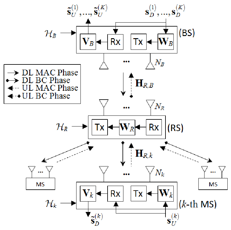
The detailed model of the system under study is shown in Fig. 3. We consider two-way relaying between one BS and KK MSs. For ease of exposition, we focus on the kk-th MS and the same model applies to all the MSs. The BS is equipped with NBN_{B} antennas, the RS is equipped with NRN_{R} antennas, and the kk-th MS is equipped with NkN_{\,k} antennas. In the DL, the BS transmits LkL_{\,k} data streams sD(k)∈ℂLk×1\textbf{s}_{D}^{(k)}\in\mathbb{C}^{\,L_{k}\times 1} to the kk-th MS and a total of L=∑k=1KLkL=\sum_{k=1}^{K}\!L_{\,k} data streams sD≜[sD(1);…;sD(K)]\textbf{s}_{D}\triangleq[\,\textbf{s}_{D}^{(1)}\,;\,\ldots\,;\,\textbf{s}_{D}^{(K)}\,] to all the MSs. In the UL, the kk-th MS transmits LkL_{\,k} data streams sU(k)∈ℂLk×1\textbf{s}_{\,U}^{(k)}\in\mathbb{C}^{\,L_{k}\times 1} to the BS, and altogether the MSs transmit LL data streams sU≜[sU(1);…;sU(K)]\textbf{s}_{\,U}\triangleq[\,\textbf{s}_{\,U}^{(1)}\,;\,\ldots\,;\,\textbf{s}_{\,U}^{(K)}\,] to the BS. We make the following assumptions about the data model.

Assumption 1 (Data Model)

All data streams are independent and have unit power. The covariance matrix of the DL data streams is given by 𝔼⁡(sD​(sD)†)=IL\mathbb{E}(\,\textbf{s}_{D}(\textbf{s}_{D})^{{\dagger}\,})=\textbf{I}_{L}, and the covariance matrix of the UL data streams is given by 𝔼⁡(sU(k)​(sU(k))†)=ILk\mathbb{E}(\,\textbf{s}_{\,U}^{(k)}(\textbf{s}_{\,U}^{(k)})^{{\dagger}\,})=\textbf{I}_{L_{k}}.  ∎

II-A Two-Way Relaying MAC Phase

In the MAC phase, the BS precodes the DL data streams sD\textbf{s}_{D} using the precoder matrix WB≜[WB,1,…,WB,K]\textbf{W}_{\!B}\triangleq[\,\textbf{W}_{\!B,1},\ldots,\textbf{W}_{\!B,K}\,], where WB,k∈ℂNB×Lk\textbf{W}_{\!B,\,k}\in\mathbb{C}^{\,N_{B}\times L_{k}} is the precoder matrix for data streams sD(k)\textbf{s}_{D}^{(k)}. Thus, the transmitted signals of the BS are given by xB=WB​sD\textbf{x}_{B}=\textbf{W}_{\!B}\,\textbf{s}_{D}. Similarly, the kk-th MS precodes the data streams sU(k)\textbf{s}_{\,U}^{(k)} using the precoder matrix Wk∈ℂNk×Lk\textbf{W}_{k}\in\mathbb{C}^{\,N_{k}\times L_{k}}, and the transmitted signals of the kk-th MS are given by xk=Wk​sU(k)\textbf{x}_{\,k}=\textbf{W}_{k}\,\textbf{s}_{\,U}^{(k)}. We make the following assumptions about the transmit power constraints of the BS and the MSs.

Assumption 2 (BS and MS Transmit Power Constraints)

The maximum transmit power of the BS is given by 𝔼⁡(‖xB‖ 2)=‖WB‖ 2≤PB\mathbb{E}(||\,\textbf{x}_{B}\,||^{\,2\,})=||\,\textbf{W}_{\!B}\,||^{\,2\,}\leq P_{B}. The maximum transmit power of the kk-th MS is given by 𝔼⁡(‖xk‖ 2)=‖Wk‖ 2≤Pk\mathbb{E}(||\,\textbf{x}_{\,k}\,||^{\,2\,})=||\,\textbf{W}_{k}\,||^{\,2\,}\leq P_{\,k}.  ∎

Let HR,B∈ℂNR×NB\textbf{H}_{R\,,B}\!\in\!\mathbb{C}^{\,N_{R}\times N_{B}} denote the channel matrix from the BS to the RS, and let HR,k∈ℂNR×Nk\textbf{H}_{R\,,\,k}\!\in\!\mathbb{C}^{\,N_{R}\times N_{k}} denote the channel matrix from the kk-th MS to the RS. It follows that the received signals of the RS can be expressed as

yR=∑m=1KHR,m​xm+HR,B​xB+nR=U​sU+D​sD+nR,\displaystyle\textstyle\textbf{y}_{\!R}=\sum_{m=1}^{K}\!\textbf{H}_{R\,,m}\,\textbf{x}_{\,m}+\textbf{H}_{R\,,B}\,\textbf{x}_{B}+\textbf{n}_{R}=\textbf{U}\,\textbf{s}_{\,U}+\textbf{D}\,\textbf{s}_{D}+\textbf{n}_{R}, (1)

where U≜[HR,1​W1,…,HR,K​WK]\textbf{U}\triangleq[\,\textbf{H}_{R\,,1}\textbf{W}_{1},\ldots,\textbf{H}_{R\,,K}\textbf{W}_{\!K}\,] and D≜HR,B​WB\textbf{D}\triangleq\textbf{H}_{R\,,B}\textbf{W}_{\!B} represent the MAC phase effective channel matrices of the UL and DL data streams, respectively, and nR∼𝒞​𝒩​(0NR×1,N 0​INR)\textbf{n}_{R}\sim\mathcal{CN}\big(\textbf{0}_{N_{R}\times 1},N_{\,0}\,\textbf{I}_{N_{R}}\big) is the AWGN. We make the following assumptions about the channel model.

Assumption 3 (Channel Model)

All channels are independent and exhibit quasi-static fading such that the channel matrices {HR,1,…,HR,K,HR,B}\{\textbf{H}_{R\,,1},\ldots,\textbf{H}_{R\,,K},\textbf{H}_{R\,,B}\} remain unchanged during a fading block of two time slots spanning the MAC and BC phases. Moreover, the forward and reverse channels are reciprocal: the channel matrix from the RS to the kk-th MS is given by (HR,k)T(\textbf{H}_{R\,,\,k})^{T}, and the channel matrix from the RS to the BS is given by (HR,B)T(\textbf{H}_{R\,,B})^{T}. Without loss of generality, we assume rank​(HR,k)≥Lk\textrm{rank}(\textbf{H}_{R\,,\,k})\geq L_{\,k} and rank​(HR,B)≥L\textrm{rank}(\textbf{H}_{R\,,B})\geq L.  ∎

II-B Two-Way Relaying BC Phase

In the BC phase, the RS amplifies the received signals yR\textbf{y}_{\!R} using the transformation matrix WR∈ℂNR×NR\textbf{W}_{\!R}\in\mathbb{C}^{\,N_{R}\times N_{R}}, and the forwarded signals are given by

xR=WR​yR=WR​U​sU+WR​D​sD+WR​nR.\displaystyle\textbf{x}_{R}=\textbf{W}_{\!R}\,\textbf{y}_{\!R}=\textbf{W}_{\!R}\,\textbf{U}\,\textbf{s}_{\,U}+\textbf{W}_{\!R}\,\textbf{D}\,\textbf{s}_{D}+\textbf{W}_{\!R}\,\textbf{n}_{R}. (2)

We make the following assumption about the transmit power constraint of the RS.

Assumption 4 (RS Transmit Power Constraint)

The maximum transmit power of the RS is given by 𝔼⁡(‖xR‖ 2)=∑m=1K‖WR​HR,m​Wm‖ 2+‖WR​HR,B​WB‖2+N 0​‖WR‖ 2≤PR\mathbb{E}(||\,\textbf{x}_{R}\,||^{\,2\,})=\sum_{m=1}^{K}\!||\,\textbf{W}_{\!R}\,\textbf{H}_{R\,,m}\textbf{W}_{m}\,||^{\,2\,}+||\,\textbf{W}_{\!R}\,\textbf{H}_{R\,,B}\textbf{W}_{\!B}\,||^{2\,}+N_{\,0}||\,\textbf{W}_{\!R}\,||^{\,2\,}\leq P_{R}.   ∎

Accordingly, the received signals of the BS are given by

yB=(HR,B)T​xR+nB=(HR,B)T​WR​U​sU⏟desired signals+(HR,B)T​WR​nR+nB⏟aggregate noise+iB,\displaystyle\textbf{y}_{\!B}=(\textbf{H}_{R\,,B})^{T}\textbf{x}_{R}+\textbf{n}_{B}=\underbrace{(\textbf{H}_{R\,,B})^{T\,}\textbf{W}_{\!R}\,\textbf{U}\,\textbf{s}_{\,U}}_{\textrm{desired signals}}+\underbrace{(\textbf{H}_{R\,,B})^{T\,}\textbf{W}_{\!R}\;\textbf{n}_{R}+\textbf{n}_{B}}_{\textrm{aggregate noise}}+\;\textbf{i}_{B}, (3)

where nB∼𝒞​𝒩​(0NB×1,N 0​INB)\textbf{n}_{B}\sim\mathcal{CN}\big(\textbf{0}_{N_{B}\times 1},N_{\,0}\,\textbf{I}_{N_{B}}\big) is the AWGN and iB≜(HR,B)T​WR​D​sD\textbf{i}_{B}\triangleq(\textbf{H}_{R\,,B})^{T\,}\textbf{W}_{\!R}\,\textbf{D}\,\textbf{s}_{D} is the backward propagated self-interference. Likewise, the received signals of the kk-th MS are given by

yk\displaystyle\textbf{y}_{k} =(HR,k)T​xR+nk\displaystyle\;=(\textbf{H}_{R\,,\,k})^{T}\textbf{x}_{R}+\textbf{n}_{k} (4)
=(HR,k)T​WR​HR,B​WB,k​sD(k)⏟desired signals+(HR,k)T​WR​(D~k​sD+U~k​sU)⏟multi-user interference+(HR,k)T​WR​nR+nk⏟aggregate noise+ik,\displaystyle\;=\underbrace{(\textbf{H}_{R\,,\,k})^{T\,}\textbf{W}_{\!R}\,\textbf{H}_{R\,,B}\textbf{W}_{\!B,\,k}\,\textbf{s}_{D}^{(k)}}_{\textrm{desired signals}}+\underbrace{(\textbf{H}_{R\,,\,k})^{T\,}\textbf{W}_{\!R\,}(\widetilde{\textbf{D}}_{k\,}\textbf{s}_{D}+\widetilde{\textbf{U}}_{k\,}\textbf{s}_{\,U})}_{\textrm{multi-user interference}}+\underbrace{(\textbf{H}_{R\,,\,k})^{T\,}\textbf{W}_{\!R}\;\textbf{n}_{R}+\textbf{n}_{\,k}}_{\textrm{aggregate noise}}+\;\textbf{i}_{\,k},

where nk∼𝒞​𝒩​(0Nk×1,N 0​INk)\textbf{n}_{\,k}\sim\mathcal{CN}\big(\textbf{0}_{N_{k}\times 1},N_{\,0}\,\textbf{I}_{N_{k}}\big) is the AWGN, ik≜(HR,k)T​WR​HR,k​Wk​sU(k)\textbf{i}_{\,k}\triangleq(\textbf{H}_{R\,,\,k})^{T\,}\textbf{W}_{\!R}\;\textbf{H}_{R\,,\,k}\textbf{W}_{k}\,\textbf{s}_{\,U}^{(k)} is the self-interference, and U~k≜[HR,1​W1,…,HR,k−1​Wk−1,0NR×Lk,HR,k+1​Wk+1,…,HR,K​WK]\widetilde{\textbf{U}}_{k}\triangleq[\,\textbf{H}_{R\,,1}\textbf{W}_{1},\ldots,\textbf{H}_{R\,,\,k-1}\textbf{W}_{k-1},\textbf{0}_{N_{R}\times L_{k}},\textbf{H}_{R\,,\,k+1}\textbf{W}_{k+1},\ldots,\textbf{H}_{R\,,K}\textbf{W}_{\!K}\,] and D~k≜HR,B​[WB,1,…,WB,k−1,0NB×Lk,WB,k+1,…,WB,K]\widetilde{\textbf{D}}_{k}\triangleq\textbf{H}_{\,R,B}\>[\,\textbf{W}_{\!B,1},\ldots,\textbf{W}_{\!B,\,k-1},\textbf{0}_{N_{B}\times L_{k}},\textbf{W}_{\!B,\,k+1},\ldots,\textbf{W}_{\!B,K}\,] are the MAC phase effective channel matrices of the UL and DL interference streams, respectively.

II-C Receive Processing

The BS and MS receive processing consists of two steps. Inherent to the two-way relaying protocol, the BS and the MSs can exploit the a priori knowledge of their own transmitted signals to cancel the backward propagated self-interference22 2 We shall elaborate in Section IV-D the assumptions on the side information available at each node to facilitate transceiver design and self-interference cancelation.. After that, the BS and the MSs process the resultant signals using linear equalizers to produce data stream estimates. Specifically, the BS cancels the self-interference iB\textbf{i}_{B} from the received signals yB\textbf{y}_{\!B} and processes them using the equalizer matrix VB≜[VB(1);…;VB(K)]\textbf{V}_{\!B}\triangleq[\,\textbf{V}_{\!B}^{\,(1)}\,;\,\ldots\,;\,\textbf{V}_{\!B}^{\,(K)}\,], where VB(k)∈ℂLk×NB\textbf{V}_{\!B}^{\,(k)}\in\mathbb{C}^{\,L_{k}\times N_{B}} is the equalizer matrix for data streams sU(k)\textbf{s}_{\,U}^{(k)}. The UL data stream estimates are given by

s~U=VB​(yB−iB)=[s~U(1);…;s~U(K)],\displaystyle\widetilde{\textbf{s}}_{\,U}=\textbf{V}_{\!B}\,(\,\textbf{y}_{\!B}\!-\textbf{i}_{B}\,)=[\,\widetilde{\textbf{s}}_{\,U}^{\,(1)}\,;\,\ldots\,;\,\widetilde{\textbf{s}}_{\,U}^{\,(K)}\,],
s~U(k)=VB(k)​(HR,B)T​WR​U​sU+VB(k)​(HR,B)T​WR​nR+VB(k)​nB.\displaystyle\widetilde{\textbf{s}}_{\,U}^{\,(k)}=\textbf{V}_{\!B}^{\,(k)}(\textbf{H}_{R\,,B})^{T\,}\textbf{W}_{\!R}\,\textbf{U}\,\textbf{s}_{\,U}+\textbf{V}_{\!B}^{\,(k)}(\textbf{H}_{R\,,B})^{T\,}\textbf{W}_{\!R}\,\textbf{n}_{R}\!+\!\textbf{V}_{\!B}^{\,(k)}\,\textbf{n}_{B}.\;\;\;

In the same way, the kk-th MS cancels the self-interference ik\textbf{i}_{\,k} from the received signals yk\textbf{y}_{k} and processes them using the equalizer matrix Vk∈ℂLk×Nk\textbf{V}_{k}\in\mathbb{C}^{\,L_{k}\times N_{k}} to produce the DL data stream estimates

s~D(k)=Vk​(yk−ik)\displaystyle\widetilde{\textbf{s}}_{D}^{\,(k)}=\textbf{V}_{k}\,(\,\textbf{y}_{k}\!-\textbf{i}_{\,k}\,) (7)
=Vk​(HR,k)T​WR​HR,B​WB,k​sD(k)+Vk​(HR,k)T​WR​(D~k​sD+U~k​sU)+Vk​(HR,k)T​WR​nR+Vk​nk.\displaystyle=\!\textbf{V}_{k}(\textbf{H}_{R\,,\,k})^{T\,}\textbf{W}_{\!R}\,\textbf{H}_{R\,,B}\textbf{W}_{\!B,\,k}\,\textbf{s}_{D}^{(k)}\!+\!\textbf{V}_{k}(\textbf{H}_{R\,,\,k})^{T\,}\textbf{W}_{\!R\,}(\widetilde{\textbf{D}}_{k\,}\textbf{s}_{D}\!+\!\widetilde{\textbf{U}}_{k\,}\textbf{s}_{\,U})\!+\!\textbf{V}_{k}(\textbf{H}_{R\,,\,k})^{T\,}\textbf{W}_{\!R}\;\textbf{n}_{R}\!+\!\textbf{V}_{k}\,\textbf{n}_{\,k}.

In the UL the SINR of the data stream estimate [s~U(k)](l)[\,\widetilde{\textbf{s}}_{\,U}^{\,(k)}\,]_{(l)} is given by

γU(k,l)≜|[VB(k)](l,:)(HR,B)TWRHR,k[Wk](:,l)| 2(||[VB(k)](l,:)(HR,B)TWRU|| 2−|[VB(k)](l,:)(HR,B)TWRHR,k[Wk](:,l)| 2+N 0(||[VB(k)](l,:)(HR,B)TWR|| 2+||[VB(k)](l,:)|| 2)),\displaystyle\gamma_{\,U}^{(k,\,l)}\triangleq\frac{\begin{subarray}{c}\textstyle|\,[\,\textbf{V}_{\!B}^{\,(k)}\,]_{(l,\,:)}(\textbf{H}_{R\,,B})^{T\,}\textbf{W}_{\!R}\,\textbf{H}_{R\,,\,k}\,[\,\textbf{W}_{k}\,]_{(:,\,l)}\,|^{\,2\,}\end{subarray}}{\left(\begin{subarray}{c}\textstyle||\,[\,\textbf{V}_{\!B}^{\,(k)}\,]_{(l,\,:)}(\textbf{H}_{R\,,B})^{T\,}\textbf{W}_{\!R}\,\textbf{U}\,||^{\,2\,}-\textstyle|\,[\,\textbf{V}_{\!B}^{\,(k)}\,]_{(l,\,:)}(\textbf{H}_{R\,,B})^{T\,}\textbf{W}_{\!R}\,\textbf{H}_{R\,,\,k}\,[\,\textbf{W}_{k}\,]_{(:,\,l)}\,|^{\,2\,}\\ \textstyle+N_{\,0}(||\,[\,\textbf{V}_{\!B}^{\,(k)}\,]_{(l,\,:)}(\textbf{H}_{R\,,B})^{T\,}\textbf{W}_{\!R}\,||^{\,2\,}+||\,[\,\textbf{V}_{\!B}^{\,(k)}\,]_{(l,\,:)}\,||^{\,2\,})\end{subarray}\right)}, (8)

and in the DL the SINR of the data stream estimate [s~D(k)](l)[\,\widetilde{\textbf{s}}_{D}^{\,(k)}\,]_{(l)} is given by

γD(k,l)≜|[Vk](l,:)(HR,k)TWRHR,B[WB,k](:,l)| 2(||[Vk](l,:)(HR,k)TWR[D,U~k]|| 2−|[Vk](l,:)(HR,k)TWRHR,B[WB,k](:,l)| 2+N 0(||[Vk](l,:)(HR,k)TWR|| 2+||[Vk](l,:)|| 2)).\displaystyle\gamma_{D}^{(k,\,l)}\triangleq\frac{\begin{subarray}{c}\textstyle|\,[\,\textbf{V}_{k}\,]_{(l,\,:)}(\textbf{H}_{R\,,\,k})^{T\,}\textbf{W}_{\!R}\,\textbf{H}_{R\,,B}\,[\,\textbf{W}_{\!B,\,k}\,]_{(:,\,l)}\,|^{\,2\,}\end{subarray}}{\left(\begin{subarray}{c}\textstyle||\,[\,\textbf{V}_{k}\,]_{(l,\,:)}(\textbf{H}_{R\,,\,k})^{T\,}\textbf{W}_{\!R}\,[\,\textbf{D},\widetilde{\textbf{U}}_{k}\,]\,||^{\,2\,}\!-|\,[\,\textbf{V}_{k}\,]_{(l,\,:)}(\textbf{H}_{R\,,\,k})^{T\,}\textbf{W}_{\!R}\,\textbf{H}_{R\,,B}\,[\,\textbf{W}_{\!B,\,k}\,]_{(:,\,l)}\,|^{\,2\,}\\ \textstyle+N_{\,0}(||\,[\,\textbf{V}_{k}\,]_{(l,\,:)}(\textbf{H}_{R\,,\,k})^{T\,}\textbf{W}_{\!R}\,||^{\,2\,}\!+||\,[\,\textbf{V}_{k}\,]_{(l,\,:)}\,||^{\,2\,})\end{subarray}\right)}.\;\;\;\; (9)

Furthermore, the achievable data rate for each data stream can be expressed as

UL: CU(k,l)=12log2(1+γU(k,l)),DL: CD(k,l)=12log2(1+γD(k,l)),\displaystyle\textrm{UL: }C_{\,U}^{\,(k,\,l)}=\frac{1}{2}\log_{2}(1+\gamma_{\,U}^{(k,\,l)}),\;\textrm{DL: }C_{D}^{\,(k,\,l)}=\frac{1}{2}\log_{2}(1+\gamma_{D}^{(k,\,l)}), (10)

where the factor of 1/21/2 accounts for the half-duplex loss.

III Interference Management and Transceiver Design Problem Formulation

In this section, we first discuss the motivations behind the interference management model to exploit signal space alignment. We then proceed to formulate the transceiver design problem.

III-A Interference Management via Signal Space Alignment

As shown in (II-C) and (7), the UL and DL data stream estimates are given by

s~U(k)=VB(k)​(HR,B)T​WR​U​sU+VB(k)​(HR,B)T​WR​nR+VB(k)​nB,\displaystyle\widetilde{\textbf{s}}_{\,U}^{\,(k)}\!=\!\textbf{V}_{\!B}^{\,(k)}(\textbf{H}_{R\,,B})^{T\,}\textbf{W}_{\!R}\,\textbf{U}\,\textbf{s}_{\,U}+\textbf{V}_{\!B}^{\,(k)}(\textbf{H}_{R\,,B})^{T\,}\textbf{W}_{\!R}\,\textbf{n}_{R}+\textbf{V}_{\!B}^{\,(k)}\,\textbf{n}_{B},
s~D(k)=Vk​(HR,k)T​WR​HR,B​WB,k​sD(k)⏟desired signals+Vk​(HR,k)T​WR​(D~k​sD+U~k​sU)⏟multi-user interference+Vk(HR,k)TWRnR+Vknk,\displaystyle\widetilde{\textbf{s}}_{D}^{\,(k)}\!=\!\underbrace{\textbf{V}_{k}(\textbf{H}_{R\,,\,k})^{T\,}\textbf{W}_{\!R}\,\textbf{H}_{R\,,B}\textbf{W}_{\!B,\,k}\,\textbf{s}_{D}^{(k)}}_{\textrm{desired signals}}\!+\!\underbrace{\textbf{V}_{k}(\textbf{H}_{R\,,\,k})^{T\,}\textbf{W}_{\!R\,}(\widetilde{\textbf{D}}_{k\,}\textbf{s}_{D}\!+\!\widetilde{\textbf{U}}_{k\,}\textbf{s}_{\,U})}_{\textrm{multi-user interference}}\!+\textbf{V}_{k}(\textbf{H}_{R\,,\,k})^{T\,}\textbf{W}_{\!R}\;\textbf{n}_{R}\!+\!\textbf{V}_{k}\,\textbf{n}_{\,k},

where the DL data stream estimates s~D(k)\widetilde{\textbf{s}}_{D}^{\,(k)} are prone to multi-user interference and it is nontrivial to mitigate its effects. On the one hand, it is detrimental to performance if we naively treat the multi-user interference as noise since its strength could be comparable to the desired signals. On the other hand, it is not always spectrally efficient if we were to mitigate interference by solely using conventional SDMA processing at the RS [8]. Under this approach, all the signal streams that constitute the RS forwarded signals (2) must be linearly independent, which implies that rank​([WR​U,WR​D])=2​L\textrm{rank}([\,\textbf{W}_{\!R}\,\textbf{U},\textbf{W}_{\!R}\,\textbf{D}\,])=2L and the channel matrices must satisfy

Lk≤rank​(HR,k)≤Nk,∀k∈𝒦,L≤rank​(HR,B)≤NB,\displaystyle L_{\,k}\leq\textrm{rank}(\textbf{H}_{R\,,\,k})\leq N_{\,k},\;\forall k\in\mathcal{K},\;\;L\leq\textrm{rank}(\textbf{H}_{R\,,B})\leq N_{B},
2​L≤rank​(HR,k)+nullity​(HR,k),rank​(HR,B)+nullity​(HR,B)=NR,\displaystyle 2L\leq\textrm{rank}(\textbf{H}_{R\,,\,k})\!+\!\textrm{nullity}(\textbf{H}_{R\,,\,k}),\;\textrm{rank}(\textbf{H}_{R\,,B})\!+\!\textrm{nullity}(\textbf{H}_{R\,,B})=N_{R},

so the MSs (BS) can only transmit L≤NR/2L\leq N_{R}\,/2 data streams in the UL (DL).

Taking into consideration that each node is capable of canceling the backward propagated self-interference in the received signals, we can allow the self-interference to overlap with the desired signals since ultimately it does not affect the decoding of the desired signals. As such, we can facilitate interference management by perfectly aligning the UL and DL signal spaces to reduce the dimension of the multi-user interference space at each node as exemplified in Fig. 4. Mathematically, aligning the UL and DL signal spaces can be represented as

BS: range​((HR,B)T​WR​HR,m​Wm)=range​((HR,B)T​WR​HR,B​WB,m),∀m∈𝒦,\displaystyle\textrm{range}((\textbf{H}_{R\,,B})^{T\,}\textbf{W}_{\!R}\,\textbf{H}_{R\,,m}\textbf{W}_{\!m\,})=\textrm{range}((\textbf{H}_{R\,,B})^{T\,}\textbf{W}_{\!R}\,\textbf{H}_{R\,,B}\textbf{W}_{\!B,\,m\,}),\;\;\forall m\in\mathcal{K},\;\;\;\;
kk-th MS: range​((HR,k)T​WR​HR,B​WB,m)=range​((HR,k)T​WR​HR,m​Wm),∀m∈𝒦,\displaystyle\textrm{range}((\textbf{H}_{R\,,\,k})^{T\,}\textbf{W}_{\!R}\,\textbf{H}_{R\,,B}\textbf{W}_{\!B,\,m\,})=\textrm{range}((\textbf{H}_{R\,,\,k})^{T\,}\textbf{W}_{\!R}\,\textbf{H}_{R\,,m}\textbf{W}_{\!m\,}),\;\;\forall m\in\mathcal{K},\;\;\;\;

and this can be manifested by constructing the RS forwarded signals (2) such that

range​(WR​HR,m​Wm)⏟UL signals=range​(WR​HR,B​WB,m)⏟DL signals.\displaystyle\underbrace{\textrm{range}(\textbf{W}_{\!R}\,\textbf{H}_{R\,,m}\textbf{W}_{\!m\,})}_{\textrm{UL signals}}=\underbrace{\textrm{range}(\textbf{W}_{\!R}\,\textbf{H}_{R\,,B}\textbf{W}_{\!B,\,m\,})}_{\textrm{DL signals}}. (15)

In order for all the UL and DL signal streams to be linearly independent, the rank of the RS forwarded signals should be

UL: rank([WRHR,1W1,…,WRHR,KWK])=L,\displaystyle\textrm{UL: }\textrm{rank}([\,\textbf{W}_{\!R}\,\textbf{H}_{R\,,1}\textbf{W}_{1\,},\ldots,\textbf{W}_{\!R}\,\textbf{H}_{R\,,K}\textbf{W}_{\!K\,}\,])=L,
DL: rank([WRHR,BWB, 1,…,WRHR,BWB,K])=L,\displaystyle\textrm{DL: }\textrm{rank}([\,\textbf{W}_{\!R}\,\textbf{H}_{R\,,B}\textbf{W}_{\!B,\,1\,},\ldots,\textbf{W}_{\!R}\,\textbf{H}_{R\,,B}\textbf{W}_{\!B,\,K\,}\,])=L,
rank([WR​HR,1​W1,…,WR​HR,K​WK⏟UL signals,WR​HR,B​WB, 1,…,WR​HR,B​WB,K⏟DL signals])=L,\displaystyle\textrm{rank}([\,\underbrace{\textbf{W}_{\!R}\,\textbf{H}_{R\,,1}\textbf{W}_{1\,},\ldots,\textbf{W}_{\!R}\,\textbf{H}_{R\,,K}\textbf{W}_{\!K\,}\!}_{\textrm{UL signals}},\underbrace{\textbf{W}_{\!R}\,\textbf{H}_{R\,,B}\textbf{W}_{\!B,\,1\,},\ldots,\textbf{W}_{\!R}\,\textbf{H}_{R\,,B}\textbf{W}_{\!B,\,K\,}\!}_{\textrm{DL signals}}\,])=L,

and from (III-A) it suffices that the channel matrices satisfy

Lk≤rank​(HR,k)≤Nk,∀k∈𝒦,L≤rank​(HR,B)≤NB,\displaystyle L_{\,k}\leq\textrm{rank}(\textbf{H}_{R\,,\,k})\leq N_{\,k},\;\forall k\in\mathcal{K},\;\;L\leq\textrm{rank}(\textbf{H}_{R\,,B})\leq N_{B},
L≤rank​(HR,k)+nullity​(HR,k),rank​(HR,B)+nullity​(HR,B)=NR,\displaystyle L\leq\textrm{rank}(\textbf{H}_{R\,,\,k})\!+\!\textrm{nullity}(\textbf{H}_{R\,,\,k}),\;\textrm{rank}(\textbf{H}_{R\,,B})\!+\!\textrm{nullity}(\textbf{H}_{R\,,B})=N_{R},

so the MSs (BS) can transmit L≤NRL\leq N_{R} data streams in the UL (DL). Comparing (III-A) and (III-A) shows that we can achieve superior multiplexing gain by exploiting signal space alignment than by performing conventional SDMA processing.

Consider again the UL and DL data stream estimates in (II-C) and (7). Exploiting signal space alignment, in the DL data stream estimates s~D(k)\widetilde{\textbf{s}}_{D}^{\,(k)} the UL and DL multi-user interference streams span the same signal space and appear as if they were one set of streams. In effect, UL and DL transmissions perform similarly to separated one-way relaying transmissions.

Remark 1 (Feasibility of Signal Space Alignment)

Aligning the UL and DL signal spaces as per (15) requires that the two-way signals between the BS and the kk-th MS be aligned when received by the RS (i.e., a single node), which then broadcasts the aligned signals back to the BS and the kk-th MS. Using the arguments of coordinated transmission and reception [32], it can be shown that the alignment operation is feasible if the number of antennas and data streams for each node and the rank of the channel matrices satisfy (III-A). Note that this is unlike conventional IA for interference channels, which is subject to stringent feasibility conditions [24, 25, 26], due to the requirement to simultaneously align interference at multiple nodes.  ∎

Remark 2 (DoF of One- and Two-Way AF Relaying)

As per [33, 32], the achievable DoF of multi-user one-way half-duplex AF relaying is 1/2​min⁡{rank​(HR,B),rank​([HR,1,…,HR,K])}1/2\min\{\textrm{rank}(\textbf{H}_{R\,,B}),\textrm{rank}([\,\textbf{H}_{R\,,1},\ldots,\textbf{H}_{R\,,K}\,])\}, where the factor of 1/21/2 accounts for the half-duplex loss. Exploiting signal space alignment, the achievable DoF of two-way relaying is min⁡{rank​(HR,B),rank​([HR,1,…,HR,K])}\min\{\textrm{rank}(\textbf{H}_{R\,,B}),\textrm{rank}([\,\textbf{H}_{R\,,1},\ldots,\textbf{H}_{R\,,K}\,])\}.  ∎

Corollary 1

For independent and identically distributed (i.i.d.) Rayleigh fading channels, with probability 1, rank​(HR,k)=min⁡{Nk,NR}\textrm{rank}(\textbf{H}_{R\,,k})=\min\{N_{\,k},N_{R}\,\}, rank​([HR,1,…,HR,K])=min⁡{NR,∑k=1KNk}\textrm{rank}([\,\textbf{H}_{R\,,1},\ldots,\textbf{H}_{R\,,K}\,])=\min\{N_{R},\sum_{k=1}^{K}\!N_{\,k}\}, and rank​(HR,B)=min⁡{NB,NR}\textrm{rank}(\textbf{H}_{R\,,B})=\min\{N_{B},N_{R}\,\}. Thus, the achievable DoF of two-way relaying is given by
min⁡{min⁡{NB,NR},min⁡{NR,∑k=1KNk}}=min⁡{NB,NR,∑k=1KNk}\min\{\min\{N_{B},N_{R}\,\},\min\{N_{R},\sum_{k=1}^{K}\!N_{\,k}\}\}=\min\{N_{B},N_{R},\sum_{k=1}^{K}\!N_{\,k}\}.  ∎

III-B Transceiver Design Optimization

In the preceding discussion, we have focused on interference management without regard for QoS considerations. In practice, the users might have different service priorities, and their data streams might have heterogenous requirements (for example, in terms of throughput and reliability). However, as shown in (8)–(10), the achievable data rate for each data stream is intricately related to the channel qualities of all links and the transceiver matrices of all nodes. One issue is that typically the transmit power of the BS is substantially higher than the MSs, and the transceiver design should accommodate for the unequal transmit powers to ensure that both UL and DL transmissions are of satisfactory performance. Toward this end, we seek to optimize the transceiver design to maximize the minimum weighted SINR among all data streams. Specifically, we associate with each UL and DL data stream a weight factor that corresponds to its priority, where the higher the priority of a data stream the larger its weight factor. In the UL let [𝝎U(k)](l)≥1[\,\boldsymbol{\omega}_{U}^{(k)}\,]_{(l)}\geq 1 denote the weight factor for data stream [sU(k)](l)[\,\textbf{s}_{\,U}^{(k)}\,]_{(l)}, and in the DL let [𝝎D(k)](l)≥1[\,\boldsymbol{\omega}_{\!D}^{(k)}\,]_{(l)}\geq 1 denote the weight factor for data stream [sD(k)](l)[\,\textbf{s}_{D}^{(k)}\,]_{(l)}. We define the weighted per stream SINRs as

UL: ([𝝎U(k)](l))−1γU(k,l),DL: ([𝝎D(k)](l))−1γD(k,l).\displaystyle\textrm{UL: }\big([\,\boldsymbol{\omega}_{U}^{(k)}\,]_{(l)}\big)^{-1}\gamma_{\,U}^{(k,\,l)},\;\textrm{DL: }\big([\,\boldsymbol{\omega}_{\!D}^{(k)}\,]_{(l)}\big)^{-1}\gamma_{D}^{(k,\,l)}. (21)

By maximizing the minimum weighted per stream SINR, we can simultaneously enhance the performance of all data streams while accounting for their relative priorities. Altogether, we formulate the two-way relaying transceiver design problem as follows.

Problem 1 (Two-Way Relaying Transceiver Design with QoS Constraints)

Given the transmit power constraint of each node and the priority weight factor of each data stream, we design the two-way relaying transceiver processing – exploiting signal space alignment – to maximize the minimum weighted per stream SINR.
{WB⋆,{Wk⋆}k=1K,WR⋆,VB⋆,{Vk⋆}k=1K}:=𝒬⁡{PB,{Pk}k=1K,PR,{𝛚U(k),𝛚D(k)}k=1K}\big\{\textbf{W}_{\!B}^{\,\star},\{\>\!\textbf{W}_{k}^{\,\star\,}\}_{k=1}^{K},\!\textbf{W}_{\!R}^{\,\star},\textbf{V}_{\!B}^{\,\star},\{\>\!\textbf{V}_{k}^{\,\star\,}\}_{k=1}^{K}\big\}:=\mathcal{Q}\big\{P_{B},\{P_{\,k}\}_{k=1}^{K},P_{R},\{\boldsymbol{\omega}_{U}^{(k)}\!,\boldsymbol{\omega}_{\!D}^{(k)\,}\}_{k=1}^{K}\big\}

(22a)
(22d)

∎

Note that Problem 𝒬\mathcal{Q} is difficult to solve since it does not lead to closed-form solutions and is non-convex. As we show in the next section, it is also nontrivial to reformulate Problem 𝒬\mathcal{Q} in order to take advantage of its structures and solve it more easily33 3 The general two-way transceiver optimization problem is extremely complex. By imposing the signal alignment structure, we can simplify the freedoms of optimization to obtain effective and pragmatic transceiver designs..

IV Proposed Solution

IV-A Two-Stage Transceiver Design Paradigm

The transceiver design problem, Problem 𝒬\mathcal{Q}, does not lead to closed-form solutions and is non-convex (since the objective function and constraints are not jointly convex in all the optimization variables); thus, we cannot efficiently solve for all the transceiver matrices in a single-shot manner. We propose to solve the transceiver design problem using a two-stage paradigm: in the first stage we focus on attaining alignment between the UL and DL signal streams, and in the second stage we aim at optimizing the weighted per stream SINRs.

To facilitate decomposing the transceiver design problem into two stages, we first extend the signal model as follows. We divide the RS transformation matrix into two components

WR≜FR​AR;\displaystyle\textbf{W}_{\!R}\triangleq\textbf{F}_{\!R\,}\textbf{A}_{R}; (22w)

we define AR≜[AR(1);…;AR(K)]\textbf{A}_{R}\triangleq[\,\textbf{A}_{R}^{\!(1)}\,;\,\ldots\,;\,\textbf{A}_{R}^{\!(K)}\,] as the RS equalizer matrix and FR≜[FR(1),…,FR(K)]\textbf{F}_{\!R}\triangleq[\,\textbf{F}_{\!R}^{\,(1)},\ldots,\textbf{F}_{\!R}^{\,(K)}\,] as the RS precoder matrix, where the submatrices AR(k)∈ℂLk×NR\textbf{A}_{R}^{\!(k)}\in\mathbb{C}^{\,L_{k}\times N_{R}} and FR(k)∈ℂNR×Lk\textbf{F}_{\!R}^{\,(k)}\in\mathbb{C}^{\,N_{R}\times L_{k}} are associated with the signal streams of the kk-th MS. Substituting (22w) into (2), the RS forwarded signals are given by xR=FR​(AR​[HR,1​W1,…,HR,K​WK]​sU+AR​[HR,B​WB,1,…,HR,B​WB,K]​sD+nR)\textbf{x}_{R}=\textbf{F}_{\!R\,}\big(\textbf{A}_{R}\,[\,\textbf{H}_{R\,,1}\textbf{W}_{1},\ldots,\textbf{H}_{R\,,K}\textbf{W}_{\!K}\,]\,\textbf{s}_{\,U}+\textbf{A}_{R}\,[\,\textbf{H}_{R\,,B}\textbf{W}_{\!B,1},\ldots,\textbf{H}_{R\,,B}\textbf{W}_{\!B,K}\,]\,\textbf{s}_{D}+\textbf{n}_{R}\big). Analogous to interference alignment (cf. [26] and references therein), aligning the UL and DL signal streams (22d) can be encompassed by the following conditions:

UL: AR(k)HR,kWk=diag(ϕ(k)),AR(k)HR,mWm=0Lk×Lm,k≠m,\displaystyle\textrm{UL: }\textbf{A}_{R}^{\!(k)}\,\textbf{H}_{R\,,\,k}\textbf{W}_{k}=\textrm{diag}(\boldsymbol{\phi}^{\,(k)}\,),\;\;\textbf{A}_{R}^{\!(k)}\,\textbf{H}_{R\,,\,m}\textbf{W}_{m}=\textbf{0}_{L_{k}\times L_{m}},\;k\neq m,
DL: AR(k)HR,BWB,k=diag(𝝍(k)),AR(k)HR,BWB,m=0Lk×Lm,k≠m.\displaystyle\textrm{DL: }\textbf{A}_{R}^{\!(k)}\,\textbf{H}_{R\,,B}\textbf{W}_{\!B,\,k}=\textrm{diag}(\boldsymbol{\psi}^{\,(k)}\,),\;\;\textbf{A}_{R}^{\!(k)}\,\textbf{H}_{R\,,B}\textbf{W}_{\!B,\,m}=\textbf{0}_{L_{k}\times L_{m}},\;k\neq m.
Remark 3 (Interpretation of (IV-A))

We design the precoder matrices WB,k\textbf{W}_{\!B,\,k} and Wk\textbf{W}_{k} such that the two-way signals between the BS and the kk-th MS are perfectly aligned at the RS and linearly independent to other users’ signals.  ∎

Accordingly, the RS forwarded signals can be expressed as

xR=FR​(𝚽​sU+𝚿​sD+AR​nR),\displaystyle\textbf{x}_{R}=\textbf{F}_{\!R\,}(\boldsymbol{\Phi}\,\textbf{s}_{\,U}+\boldsymbol{\Psi}\,\textbf{s}_{D}+\textbf{A}_{R}\,\textbf{n}_{R}\,), (22z)

where 𝚽≜diag​(ϕ(1),…,ϕ(K))\boldsymbol{\Phi}\triangleq\textrm{diag}(\boldsymbol{\phi}^{\,(1)}\!,\ldots,\boldsymbol{\phi}^{\,(K)}\,) and 𝚿≜diag​(𝝍(1),…,𝝍(K))\boldsymbol{\Psi}\triangleq\textrm{diag}(\boldsymbol{\psi}^{\,(1)}\!,\ldots,\boldsymbol{\psi}^{\,(K)}\,) represent the effective gains of the UL and DL data streams, respectively. The transmit power constraint of the RS forwarded signals is given by 𝔼⁡(‖xR‖ 2)=‖FR​𝚽‖ 2+‖FR​𝚿‖ 2+N 0​‖FR​AR‖ 2≤PR\mathbb{E}(||\,\textbf{x}_{R}\,||^{\,2\,})=||\,\textbf{F}_{\!R\,}\boldsymbol{\Phi}||^{\,2\,}+||\,\textbf{F}_{\!R\,}\boldsymbol{\Psi}||^{\,2\,}+N_{\,0}||\,\textbf{F}_{\!R\,}\textbf{A}_{R}\,||^{\,2\,}\!\leq P_{R}. We define the SINRs of the RS forwarded signals as

UL: γ~U(k,l)≜|[ϕ(k)](l)| 2N 0||[AR(k)](l,:)|| 2=|[AR(k)](l,:)HR,k[Wk](:,l)| 2N 0||[AR(k)](l,:)|| 2,\displaystyle\textrm{UL: }\widetilde{\gamma}_{\,U}^{(k,\,l)}\!\triangleq\!\frac{\textstyle|\,[\,\boldsymbol{\phi}^{\,(k)}\,]_{(l)}\,|^{\,2\,}}{N_{\,0}||\,[\,\textbf{A}_{R}^{\!(k)}\,]_{(l,\,:)}\,||^{\,2\,}}\!=\!\frac{\textstyle|\,[\,\textbf{A}_{R}^{\!(k)}\,]_{(l,\,:)}\,\textbf{H}_{R\,,\,k}\,[\,\textbf{W}_{k}\,]_{(:,\,l)}\,|^{\,2\,}}{N_{\,0}||\,[\,\textbf{A}_{R}^{\!(k)}\,]_{(l,\,:)}\,||^{\,2\,}},
DL: γ~D(k,l)≜|[𝝍(k)](l)| 2N 0||[AR(k)](l,:)|| 2=|[AR(k)](l,:)HR,B[WB,k](:,l)| 2N 0||[AR(k)](l,:)|| 2.\displaystyle\textrm{DL: }\widetilde{\gamma}_{D}^{(k,\,l)}\!\triangleq\!\frac{\textstyle|\,[\,\boldsymbol{\psi}^{\,(k)}\,]_{(l)}\,|^{\,2\,}}{N_{\,0}||\,[\,\textbf{A}_{R}^{\!(k)}\,]_{(l,\,:)}\,||^{\,2\,}}\!=\!\frac{\textstyle|\,[\,\textbf{A}_{R}^{\!(k)}\,]_{(l,\,:)}\,\textbf{H}_{R\,,B\,}\,[\,\textbf{W}_{\!B,\,k}\,]_{(:,\,l)}\,|^{\,2\,}}{N_{\,0}||\,[\,\textbf{A}_{R}^{\!(k)}\,]_{(l,\,:)}\,||^{\,2\,}}.

From (22z), (3) and (4), the end-to-end received signals of the BS can be expressed as

yB=(HR,B)T​FR​𝚽​sU⏟desired signals+(HR,B)T​FR​AR​nR+nB⏟aggregate noise+iB,\displaystyle\textbf{y}_{\!B}=\underbrace{(\textbf{H}_{R\,,B})^{T\,}\textbf{F}_{\!R\,}\boldsymbol{\Phi}\,\textbf{s}_{\,U}}_{\textrm{desired signals}}+\underbrace{(\textbf{H}_{R\,,B})^{T\,}\textbf{F}_{\!R\,}\textbf{A}_{R}\,\textbf{n}_{R}+\textbf{n}_{B}}_{\textrm{aggregate noise}}+\;\textbf{i}_{B}, (22ac)

and the end-to-end received signals of the kk-th MS can be expressed as

yk\displaystyle\textbf{y}_{k} =(HR,k)T​FR(k)​𝝍(k)​sD(k)⏟desired signals+(HR,k)T​FR​(𝚿~k​sD+𝚽~k​sU)⏟multi-user interference+(HR,k)T​FR​AR​nR+nk⏟aggregate noise+ik,\displaystyle\;=\underbrace{(\textbf{H}_{R\,,\,k})^{T\,}\textbf{F}_{\!R}^{\,(k)}\boldsymbol{\psi}^{\,(k)\,}\textbf{s}_{D}^{(k)}}_{\textrm{desired signals}}+\underbrace{(\textbf{H}_{R\,,\,k})^{T\,}\textbf{F}_{\!R\,}(\widetilde{\boldsymbol{\Psi}}_{k\,}\textbf{s}_{D}\!+\!\widetilde{\boldsymbol{\Phi}}_{k\,}\textbf{s}_{\,U})}_{\textrm{multi-user interference}}+\underbrace{(\textbf{H}_{R\,,\,k})^{T\,}\textbf{F}_{\!R\,}\textbf{A}_{R}\,\textbf{n}_{R}+\!\textbf{n}_{\,k}}_{\textrm{aggregate noise}}+\;\textbf{i}_{\,k},\;\;\;\; (22ad)

where 𝚽~k≜diag​(ϕ(1),…,ϕ(k−1),0Lk×1,ϕ(k+1),…,ϕ(K))\widetilde{\boldsymbol{\Phi}}_{k}\triangleq\textrm{diag}(\boldsymbol{\phi}^{\,(1)}\!,\ldots,\boldsymbol{\phi}^{\,(k-1)}\!,\textbf{0}_{L_{k}\times 1},\boldsymbol{\phi}^{\,(k+1)}\!,\ldots,\boldsymbol{\phi}^{\,(K)}\,) represent the effective gains of the UL interference streams, and 𝚿~k≜diag​(𝝍(1),…,𝝍(k−1),0Lk×1,𝝍(k+1),…,𝝍(K))\widetilde{\boldsymbol{\Psi}}_{k}\triangleq\textrm{diag}(\boldsymbol{\psi}^{\,(1)}\!,\ldots,\boldsymbol{\psi}^{\,(k-1)}\!,\textbf{0}_{L_{k}\times 1},\boldsymbol{\psi}^{\,(k+1)}\!,\ldots,\boldsymbol{\psi}^{\,(K)}\,) represent the effective gains of the DL interference streams. Therefore, the UL and DL data stream estimates (II-C), (7) can be expressed as

s~U(k)=VB(k)​(HR,B)T​FR​𝚽​sU+VB(k)​(HR,B)T​FR​AR​nR+VB(k)​nB,\displaystyle\!\!\!\!\widetilde{\textbf{s}}_{\,U}^{\,(k)}\!=\!\textbf{V}_{\!B}^{\,(k)}(\textbf{H}_{R\,,B})^{T\,}\textbf{F}_{\!R\,}\boldsymbol{\Phi}\,\textbf{s}_{\,U}+\textbf{V}_{\!B}^{\,(k)}(\textbf{H}_{R\,,B})^{T\,}\textbf{F}_{\!R\,}\textbf{A}_{R}\,\textbf{n}_{R}+\textbf{V}_{\!B}^{\,(k)}\,\textbf{n}_{B}, (22ae)
s~D(k)=Vk​(HR,k)T​FR(k)​𝝍(k)​sD(k)+Vk​(HR,k)T​FR​(𝚿~k​sD+𝚽~k​sU)+Vk​(HR,k)T​FR​AR​nR+Vk​nk,\displaystyle\!\!\!\!\widetilde{\textbf{s}}_{D}^{\,(k)}\!=\!\textbf{V}_{k}(\textbf{H}_{R\,,\,k})^{T\,}\textbf{F}_{\!R}^{\,(k)}\boldsymbol{\psi}^{\,(k)\,}\textbf{s}_{D}^{(k)}\!+\!\textbf{V}_{k}(\textbf{H}_{R\,,\,k})^{T\,}\textbf{F}_{\!R\,}(\widetilde{\boldsymbol{\Psi}}_{k\,}\textbf{s}_{D}\!+\!\widetilde{\boldsymbol{\Phi}}_{k\,}\textbf{s}_{\,U})\!+\!\textbf{V}_{k}(\textbf{H}_{R\,,\,k})^{T\,}\textbf{F}_{\!R\,}\textbf{A}_{R}\,\textbf{n}_{R}+\!\textbf{V}_{k}\,\textbf{n}_{\,k},\;\;\;\;\;\;\; (22af)

and the end-to-end SINRs of the data stream estimates (8), (9) are equivalently given by

γU(k,l)=|[VB(k)](l,:)(HR,B)T[FR(k)](:,l)[ϕ(k)](l)| 2(||[VB(k)](l,:)(HR,B)TFR𝚽|| 2−|[VB(k)](l,:)(HR,B)T[FR(k)](:,l)[ϕ(k)](l)| 2+N 0(||[VB(k)](l,:)(HR,B)TFRAR|| 2+||[VB(k)](l,:)|| 2)),\displaystyle\gamma_{\,U}^{(k,\,l)}=\frac{\begin{subarray}{c}\textstyle|\,[\,\textbf{V}_{\!B}^{\,(k)}\,]_{(l,\,:)}(\textbf{H}_{R\,,B})^{T}[\,\textbf{F}_{\!R}^{\,(k)}\,]_{(:,\,l)}[\,\boldsymbol{\phi}^{\,(k)}\,]_{(l)}\,|^{\,2\,}\end{subarray}}{\left(\begin{subarray}{c}\textstyle||\,[\,\textbf{V}_{\!B}^{\,(k)}\,]_{(l,\,:)}(\textbf{H}_{R\,,B})^{T\,}\textbf{F}_{\!R}\,\boldsymbol{\Phi}\,||^{\,2\,}\!-|\,[\,\textbf{V}_{\!B}^{\,(k)}\,]_{(l,\,:)}(\textbf{H}_{R\,,B})^{T}[\,\textbf{F}_{\!R}^{\,(k)}\,]_{(:,\,l)}[\,\boldsymbol{\phi}^{\,(k)}\,]_{(l)}\,|^{\,2\,}\\ \textstyle+N_{\,0}(||\,[\,\textbf{V}_{\!B}^{\,(k)}\,]_{(l,\,:)}(\textbf{H}_{R\,,B})^{T\,}\textbf{F}_{\!R\,}\textbf{A}_{R}\,||^{\,2\,}\!+||\,[\,\textbf{V}_{\!B}^{\,(k)}\,]_{(l,\,:)}\,||^{\,2\,})\end{subarray}\right)}, (22ag)
γD(k,l)=|[Vk](l,:)(HR,k)T[FR(k)](:,l)[𝝍(k)](l)| 2(||[Vk](l,:)(HR,k)TFR[𝚿,𝚽~k]|| 2−|[Vk](l,:)(HR,k)T[FR(k)](:,l)[𝝍(k)](l)| 2+N 0(||[Vk](l,:)(HR,k)TFRAR|| 2+||[Vk](l,:)|| 2)).\displaystyle\gamma_{D}^{(k,\,l)}=\frac{\begin{subarray}{c}\textstyle|\,[\,\textbf{V}_{k}\,]_{(l,\,:)}(\textbf{H}_{R\,,\,k})^{T}[\,\textbf{F}_{\!R}^{\,(k)}\,]_{(:,\,l)}[\,\boldsymbol{\psi}^{\,(k)}\,]_{(l)}\,|^{\,2\,}\end{subarray}}{\left(\begin{subarray}{c}\textstyle||\,[\,\textbf{V}_{k}\,]_{(l,\,:)}(\textbf{H}_{R\,,\,k})^{T\,}\textbf{F}_{\!R}\,[\,\boldsymbol{\Psi},\widetilde{\boldsymbol{\Phi}}_{k}\,]\,||^{\,2\,}\!-|\,[\,\textbf{V}_{k}\,]_{(l,\,:)}(\textbf{H}_{R\,,\,k})^{T}[\,\textbf{F}_{\!R}^{\,(k)}\,]_{(:,\,l)}[\,\boldsymbol{\psi}^{\,(k)}\,]_{(l)}\,|^{\,2\,}\\ \textstyle+N_{\,0}(||\,[\,\textbf{V}_{k}\,]_{(l,\,:)}(\textbf{H}_{R\,,\,k})^{T\,}\textbf{F}_{\!R\,}\textbf{A}_{R}\,||^{\,2\,}\!+||\,[\,\textbf{V}_{k}\,]_{(l,\,:)}\,||^{\,2\,})\end{subarray}\right)}.\;\;\;\; (22ah)
Lemma 1 (Decomposition of Transceiver Design)

The transceiver design problem, Problem 𝒬\mathcal{Q}, can be equivalently decomposed into two stages. The first stage processing finds the BS and MS precoder matrices and the RS equalizer matrix {WB,{Wk}k=1K,AR}\big\{\textbf{W}_{\!B},\{\textbf{W}_{k}\}_{k=1}^{K},\textbf{A}_{R}\big\}, subject to the alignment conditions (IV-A), to maximize the minimum weighted SINR of the RS forwarded signals.

First Stage Processing    {WB⋆,{Wk⋆}k=1K,AR⋆}:=ℳ⁡{PB,{Pk}k=1K,{𝝎U(k),𝝎D(k)}k=1K}\big\{\textbf{W}_{\!B}^{\,\star},\{\>\!\textbf{W}_{k}^{\,\star\,}\}_{k=1}^{K},\textbf{A}_{R}^{\!\star}\big\}:=\mathcal{M}\big\{P_{B},\{P_{\,k}\}_{k=1}^{K},\{\boldsymbol{\omega}_{U}^{(k)}\!,\boldsymbol{\omega}_{\!D}^{(k)\,}\}_{k=1}^{K}\big\}

(22aia)
(22aid)

The second stage processing finds the RS precoder matrix and the BS and MS equalizer matrices {FR,VB,{Vk}k=1K}\big\{\textbf{F}_{\!R},\!\textbf{V}_{\!B},\{\textbf{V}_{k}\}_{k=1}^{K}\big\} to maximize the minimum weighted end-to-end SINR of the data stream estimates. Second Stage Processing  {FR⋆,VB⋆,{Vk⋆}k=1K}:=ℬ⁡{WB⋆,{Wk⋆}k=1K,AR⋆,PR,{𝝎U(k),𝝎D(k)}k=1K}\big\{\textbf{F}_{\!R}^{\,\star},\textbf{V}_{\!B}^{\,\star},\{\textbf{V}_{k}^{\,\star\,}\}_{k=1}^{K}\big\}\!:=\mathcal{B}\big\{\textbf{W}_{\!B}^{\,\star},\{\>\!\textbf{W}_{k}^{\,\star\,}\}_{k=1}^{K},\textbf{A}_{R}^{\!\star},P_{R},\{\boldsymbol{\omega}_{U}^{(k)}\!,\boldsymbol{\omega}_{\!D}^{(k)\,}\}_{k=1}^{K}\big\}

arg⁡maxFR,VB,{Vk}k=1K\displaystyle\!\underset{\begin{subarray}{c}\textbf{F}_{\!R},\textbf{V}_{\!B},\{\textbf{V}_{k}\}_{k=1}^{K}\end{subarray}}{\arg\max} min∀k∈𝒦∀l∈ℒk⁡{([𝝎U(k)](l))−1​γU(k,l),([𝝎D(k)](l))−1​γD(k,l)}\displaystyle\min_{\begin{subarray}{c}\forall\,k\,\in\,\mathcal{K}\\ \forall\,l\,\in\,\mathcal{L}_{k}\end{subarray}}\textstyle\big\{\big([\,\boldsymbol{\omega}_{U}^{(k)}\,]_{(l)}\big)^{-1}\gamma_{\,U}^{(k,\,l)},\big([\,\boldsymbol{\omega}_{\!D}^{(k)}\,]_{(l)}\big)^{-1}\gamma_{D}^{(k,\,l)}\,\big\} (22aiaja)
      s.t. ‖FR​𝚽‖ 2+‖FR​𝚿‖ 2+N 0​‖FR​AR‖ 2≤PR.\textstyle||\,\textbf{F}_{\!R\,}\boldsymbol{\Phi}||^{\,2\,}+||\,\textbf{F}_{\!R\,}\boldsymbol{\Psi}||^{\,2\,}+N_{\,0}||\,\textbf{F}_{\!R\,}\textbf{A}_{R}\,||^{\,2\,}\!\leq P_{R\,}. (22aiajb)
Proof:

Refer to Appendix A. ∎

The top-level steps of the proposed two-stage transceiver design are summarized in Algorithm 1 and illustrated in Fig. 5. We shall elaborate the details of the first and second stage processing in the following subsections.

IV-B First Stage Processing

To solve the first stage processing, Problem ℳ\mathcal{M}, we focus our attention on coordinative eigenmode transmission at the MSs, zero-forcing equalization at the RS, and zero-forcing transmission at the BS [34].

  • •

    MS Precoder Matrices: Let 𝒢k\mathcal{G}_{\,k} denote the set of the right singular vectors of the channel matrix HR,k\textbf{H}_{R\,,\,k}. The kk-th MS precoder matrix Wk\textbf{W}_{k} is given as [Wk](:,l)=λk(l)gk(l)[\,\textbf{W}_{k}\,]_{(:,\,l)}=\sqrt{\lambda_{\,k}^{(l)}}\textbf{g}_{\,k}^{\,(l)}, where gk(l)∈𝒢k\textbf{g}_{\,k}^{\,(l)}\in\mathcal{G}_{\,k} is the beam direction, and λk(l)\lambda_{\,k}^{(l)} is the allocated power satisfying the transmit power constraint ‖Wk‖ 2=∑l=1Lkλk(l)=Pk||\,\textbf{W}_{k}\,||^{\,2\,}=\sum_{\,l=1}^{\,L_{k}}\lambda_{\,k}^{(l)}=P_{\,k}.

  • •

    RS Equalizer Matrix: The zero-forcing equalizer matrix is given as

    AR=pinv​([HR,1​[g 1(1),…,g 1(L1)],…,HR,K​[gK(1),…,gK(LK)]]).\displaystyle\textbf{A}_{R}=\textrm{pinv}([\,\textbf{H}_{R\,,1}[\,\textbf{g}_{\,1}^{\,(1)},\ldots,\textbf{g}_{\,1}^{\,(L_{1})}\,],\ldots,\textbf{H}_{R\,,K\,}[\,\textbf{g}_{K}^{\,(1)},\ldots,\textbf{g}_{K}^{\,(L_{K})}\,]\,]). (22aiak)
  • •

    BS Precoder Matrix: Let A~R(k,l)\widetilde{\textbf{A}}_{R}^{(k,\,l)} denote the matrix obtained by removing [AR(k)](l,:)[\,\textbf{A}_{R}^{\!(k)}\,]_{(l,\,:)} from AR\textbf{A}_{R} and let 𝒢B(k,l)=null​(A~R(k,l)​HR,B)\mathcal{G}_{B}^{\,(k,\,l)}=\textrm{null}(\widetilde{\textbf{A}}_{R}^{(k,\,l)\,}\textbf{H}_{R\,,B\,}). The BS precoder matrix WB\textbf{W}_{\!B} is given as [WB,k](:,l)=λB(k,l)gB(k,l)[\,\textbf{W}_{\!B,\,k}\,]_{(:,\,l)}=\sqrt{\lambda_{B}^{(k,\,l)}}\textbf{g}_{B}^{\,(k,\,l)}, where gB(k,l)∈𝒢B(k,l)\textbf{g}_{B}^{\,(k,\,l)}\in\mathcal{G}_{B}^{\,(k,\,l)} is the beam direction, and λB(k,l)\lambda_{B}^{(k,\,l)} is the allocated power satisfying the transmit power constraint ‖WB‖ 2=∑k=1K∑l=1LkλB(k,l)=PB||\,\textbf{W}_{\!B}\,||^{\,2\,}=\sum_{k=1}^{K}\sum_{\,l=1}^{\,L_{k}}\lambda_{B}^{(k,\,l)}=P_{B}.

As such, the SINRs of the RS forwarded signals (IV-A) can be equivalently expressed as

γ~U(k,l)=κU(k,l)​λk(l),γ~D(k,l)=κD(k,l)​λB(k,l),\displaystyle\widetilde{\gamma}_{\,U}^{(k,\,l)}=\kappa_{\,U}^{(k,\,l)}\lambda_{\,k}^{(l)},\;\;\widetilde{\gamma}_{D}^{(k,\,l)}=\kappa_{D}^{(k,\,l)}\lambda_{B}^{(k,\,l)}, (22aial)

where κU(k,l)≜|[AR(k)](l,:)HR,kgk(l)| 2N 0||[AR(k)](l,:)|| 2\kappa_{\,U}^{(k,\,l)}\triangleq\frac{\textstyle|\,[\,\textbf{A}_{R}^{\!(k)}\,]_{(l,\,:)}\,\textbf{H}_{R\,,\,k}\,\textbf{g}_{\,k}^{\,(l)}\,|^{\,2}}{\textstyle N_{\,0}||\,[\,\textbf{A}_{R}^{\!(k)}\,]_{(l,\,:)}\,||^{\,2}} and κD(k,l)≜|[AR(k)](l,:)HR,BgB(k,l)| 2N 0||[AR(k)](l,:)|| 2\kappa_{D}^{(k,\,l)}\triangleq\frac{\textstyle|\,[\,\textbf{A}_{R}^{\!(k)}\,]_{(l,\,:)}\,\textbf{H}_{R\,,B\,}\,\textbf{g}_{B}^{\,(k,\,l)}\,|^{\,2}}{\textstyle N_{\,0}||\,[\,\textbf{A}_{R}^{\!(k)}\,]_{(l,\,:)}\,||^{\,2}}.

Lemma 2 (Beam Directions and Power Allocation at the BS and MSs)

To maximize the minimum weighted SINR of the RS forwarded signals, the power allocation at the BS and MSs are, respectively, given by

(λB(k,l))⋆=[𝝎D(k)](l)​(κD(k,l))−1​PB∑m=1K∑q=1Lm[𝝎D(m)](q)​(κD(m,q))−1,(λk(l))⋆=[𝝎U(k)](l)​(κU(k,l))−1​Pk∑q=1Lk[𝝎U(k)](q)​(κU(k,q))−1.\displaystyle\big(\lambda_{B}^{(k,\,l)}\big)^{\!\star}\!\!=\!\!\frac{\textstyle[\,\boldsymbol{\omega}_{\!D}^{(k)}\,]_{(l)}\big(\kappa_{D}^{(k,\,l)}\big)^{-1}P_{B}}{\textstyle\sum_{m=1}^{K}\!\sum_{\,q=1}^{\,L_{m}}\,[\,\boldsymbol{\omega}_{\!D}^{(m)}\,]_{(q)}\big(\kappa_{D}^{(m,\,q)}\big)^{-1}},\;\;\big(\lambda_{\,k}^{(l)}\big)^{\!\star}\!\!=\!\!\frac{\textstyle[\,\boldsymbol{\omega}_{U}^{(k)}\,]_{(l)}\big(\kappa_{\,U}^{(k,\,l)}\big)^{-1}P_{\,k}}{\textstyle\sum_{\,q=1}^{\,L_{k}}\,[\,\boldsymbol{\omega}_{U}^{(k)}\,]_{(q)}\big(\kappa_{\,U}^{(k,\,q)}\big)^{-1}}. (22aiam)

It follows that the weighted SINRs of the RS forwarded signals can be expressed as

UL: ([𝝎U(k)](l))−1γ~U(k,l)=Pk∑q=1Lk[𝝎U(k)](q)​(κU(k,q))−1,\displaystyle\textrm{UL: }\big([\,\boldsymbol{\omega}_{U}^{(k)}\,]_{(l)}\big)^{-1}\widetilde{\gamma}_{\,U}^{(k,\,l)}\!=\!\frac{P_{\,k}}{\sum_{\,q=1}^{\,L_{k}}\,[\,\boldsymbol{\omega}_{U}^{(k)}\,]_{(q)}\big(\kappa_{\,U}^{(k,\,q)}\big)^{-1}},
DL: ([𝝎D(k)](l))−1γ~D(k,l)=PB∑m=1K∑q=1Lm[𝝎D(m)](q)​(κD(m,q))−1,\displaystyle\textrm{DL: }\big([\,\boldsymbol{\omega}_{\!D}^{(k)}\,]_{(l)}\big)^{-1}\widetilde{\gamma}_{D}^{(k,\,l)}\!=\!\frac{P_{B}}{\sum_{m=1}^{K}\sum_{\,q=1}^{\,L_{m}}\,[\,\boldsymbol{\omega}_{\!D}^{(m)}\,]_{(q)}\big(\kappa_{D}^{(m,\,q)}\big)^{-1}},

and selection of the beam directions to maximize the minimum weighted SINR can be performed using combinatorial search.

Proof:

Refer to Appendix B. ∎

IV-C Second Stage Processing

We now proceed to describe the algorithm for solving the second stage processing, Problem ℬ\mathcal{B}. As per (22ag)-(22ah), the SINRs of the data stream estimates are not jointly convex in the RS precoder matrix and the BS and MS equalizer matrices {FR,VB,{Vk}k=1K}\big\{\textbf{F}_{\!R},\!\textbf{V}_{\!B},\{\textbf{V}_{k}\}_{k=1}^{K}\big\}. However, for a fixed precoder matrix FR\textbf{F}_{\!R\,} there are closed-form solutions for the equalizer matrices VB\textbf{V}_{\!B} and Vk\textbf{V}_{k}; conversely, for fixed VB\textbf{V}_{\!B} and Vk\textbf{V}_{k} we can cast the problem of solving for FR\textbf{F}_{\!R\,} as a quasi-convex problem. This motivates the approach to progressively refine the transceiver matrices by iteratively alternate between solving for the BS and MS equalizer matrices and the RS precoder matrix. In this regard, we alternatingly optimize each one of the RS precoder matrix and the BS and MS equalizer matrices in the form of the following subproblems, and the convergence proof is provided in Appendix C. RS Precoder Matrix  {FR⋆,γ0}:=ℬR​{VB,{Vk}k=1K,WB⋆,{Wk⋆}k=1K,AR⋆,PR,{𝝎U(k),𝝎D(k)}k=1K}\big\{\textbf{F}_{\!R}^{\,\star},\gamma_{0}\big\}\!:=\mathcal{B}_{R}\big\{\textbf{V}_{\!B},\{\textbf{V}_{k}\}_{k=1}^{K},\textbf{W}_{\!B}^{\,\star},\{\>\!\textbf{W}_{k}^{\,\star\,}\}_{k=1}^{K},\textbf{A}_{R}^{\!\star},P_{R},\{\boldsymbol{\omega}_{U}^{(k)}\!,\boldsymbol{\omega}_{\!D}^{(k)\,}\}_{k=1}^{K}\big\}

(22aiapa)
(22aiapc)

BS Equalizer  VB⋆:=ℬB​{FR,WB⋆,{Wk⋆}k=1K,AR⋆,{𝝎U(k)}k=1K}\textbf{V}_{\!B}^{\,\star}:=\mathcal{B}_{B}\big\{\textbf{F}_{\!R},\textbf{W}_{\!B}^{\,\star},\{\>\!\textbf{W}_{k}^{\,\star\,}\}_{k=1}^{K},\textbf{A}_{R}^{\!\star},\{\boldsymbol{\omega}_{U}^{(k)}\}_{k=1}^{K}\big\}

arg⁡maxVB\displaystyle\!\!\underset{\textbf{V}_{\!B}}{\arg\max} min∀k∈𝒦∀l∈ℒk⁡{([𝝎U(k)](l))−1​γU(k,l)}\displaystyle\min_{\begin{subarray}{c}\forall\,k\,\in\,\mathcal{K}\\ \forall\,l\,\in\,\mathcal{L}_{k}\end{subarray}}\textstyle\big\{\big([\,\boldsymbol{\omega}_{U}^{(k)}\,]_{(l)}\big)^{-1}\gamma_{\,U}^{(k,\,l)}\big\}. (22aiapaq)

kk-th MS Equalizer Vk⋆:=ℬk​{FR,WB⋆,{Wk⋆}k=1K,AR⋆,𝝎D(k)}\textbf{V}_{k}^{\,\star\,}:=\mathcal{B}_{k}\big\{\textbf{F}_{\!R},\textbf{W}_{\!B}^{\,\star},\{\>\!\textbf{W}_{k}^{\,\star\,}\}_{k=1}^{K},\textbf{A}_{R}^{\!\star},\boldsymbol{\omega}_{\!D}^{(k)}\big\}

arg⁡maxVk\displaystyle\!\!\underset{\textbf{V}_{\!k}}{\arg\max} min∀l∈ℒk⁡{([𝝎D(k)](l))−1​γD(k,l)}\displaystyle\min_{\begin{subarray}{c}\forall\,l\,\in\,\mathcal{L}_{k}\end{subarray}}\textstyle\big\{\big([\,\boldsymbol{\omega}_{\!D}^{(k)}\,]_{(l)}\big)^{-1}\gamma_{D}^{(k,\,l)}\big\}. (22aiapar)

First, for Problem ℬB\mathcal{B}_{B} and Problem ℬk\mathcal{B}_{k}, the per stream SINRs are maximized with a minimum mean squared error (MMSE) equalizer matrix [35]. Hence, the BS equalizer matrix is given by

VB⋆=((HR,B)T​FR​𝚽)†​((HR,B)T​FR​𝚽​((HR,B)T​FR​𝚽)†+𝛀B)−1,\displaystyle\textbf{V}_{\!B}^{\,\star}=\big((\textbf{H}_{R\,,B})^{T\,}\textbf{F}_{\!R}\,\boldsymbol{\Phi}\big)^{\!{\dagger}\,}\big((\textbf{H}_{R\,,B})^{T\,}\textbf{F}_{\!R}\,\boldsymbol{\Phi}\big((\textbf{H}_{R\,,B})^{T\,}\textbf{F}_{\!R}\,\boldsymbol{\Phi}\big)^{\!{\dagger}}+\boldsymbol{\Omega}_{B}\big)^{-1}, (22aiapas)

where 𝛀B≜N 0​(HR,B)T​FR​AR​((HR,B)T​FR​AR)†+N 0​INB\boldsymbol{\Omega}_{B}\triangleq N_{\,0}(\textbf{H}_{R\,,B})^{T\,}\textbf{F}_{\!R\,}\textbf{A}_{R}\big((\textbf{H}_{R\,,B})^{T\,}\textbf{F}_{\!R\,}\textbf{A}_{R}\big)^{\!{\dagger}}+N_{\,0}\,\textbf{I}_{N_{B}} is the covariance matrix of the aggregate noise at the BS. Likewise, the kk-th MS equalizer matrix is given by

Vk⋆=((HR,k)T​FR(k)​𝝍(k))†​((HR,k)T​FR​[𝚿,𝚽~k]​((HR,k)T​FR​[𝚿,𝚽~k])†+𝛀k)−1,\displaystyle\textbf{V}_{k}^{\,\star\,}=\big((\textbf{H}_{R\,,\,k})^{T\,}\textbf{F}_{\!R}^{\,(k)}\boldsymbol{\psi}^{\,(k)}\big)^{\!{\dagger}\,}\big((\textbf{H}_{R\,,\,k})^{T\,}\textbf{F}_{\!R}\,[\,\boldsymbol{\Psi},\widetilde{\boldsymbol{\Phi}}_{k}\,]\big((\textbf{H}_{R\,,\,k})^{T\,}\textbf{F}_{\!R}\,[\,\boldsymbol{\Psi},\widetilde{\boldsymbol{\Phi}}_{k}\,]\big)^{\!{\dagger}}+\boldsymbol{\Omega}_{\,k}\big)^{-1}, (22aiapat)

where 𝛀k≜N 0​(HR,k)T​FR​AR​((HR,k)T​FR​AR)†+N 0​INk\boldsymbol{\Omega}_{\,k}\triangleq N_{\,0}(\textbf{H}_{R\,,\,k})^{T\,}\textbf{F}_{\!R\,}\textbf{A}_{R}\big((\textbf{H}_{R\,,\,k})^{T\,}\textbf{F}_{\!R\,}\textbf{A}_{R}\big)^{\!{\dagger}}+N_{\,0}\,\textbf{I}_{N_{k}} is the covariance matrix of the aggregate noise at the kk-th MS.

Second, note that Problem ℬR\mathcal{B}_{R} corresponds to designing precoders for LL two-user multicast groups, where the precoder [FR(k)](:,l)[\,\textbf{F}_{\!R}^{\,(k)}\,]_{(:,\,l)} is used for multicasting the signal stream that encapsulates the UL data stream [sU(k)](l)[\,\textbf{s}_{\,U}^{\,(k)}\,]_{(l)} and the DL data stream [sD(k)](l)[\,\textbf{s}_{D}^{\,(k)}\,]_{(l)}. As per [30, Claim 2], this multigroup multicast problem is NP-hard44 4 Please refer to [36, 37] for discussion on the unicast precoder design problem, which is not NP-hard.. We propose to solve for the RS precoder matrix FR\textbf{F}_{\!R} using Algorithm 2 as derived in Appendix D. In a nutshell, we cast Problem ℬR\mathcal{B}_{R} as a quasi-convex problem and solve it using the bisection method [31, Section 4.2.5]. To do so, we define the SOCP feasibility problem of designing FR\textbf{F}_{\!R} that achieves a target value of the minimum weighted per stream SINR γ 0\gamma_{\,0} as55 5 Due to page limit, please refer to Appendix D for the expressions for () and (22aiapauc).          FR⋆:=ℬ~R​{γ 0,VB,{Vk}k=1K,WB⋆,{Wk⋆}k=1K,AR⋆,PR,{𝝎U(k),𝝎D(k)}k=1K}\textbf{F}_{\!R}^{\,\star}:=\widetilde{\mathcal{B}}_{R}\big\{\gamma_{\,0},\!\textbf{V}_{\!B},\{\textbf{V}_{k}\}_{k=1}^{K},\textbf{W}_{\!B}^{\,\star},\{\>\!\textbf{W}_{k}^{\,\star\,}\}_{k=1}^{K},\textbf{A}_{R}^{\!\star},P_{R},\{\boldsymbol{\omega}_{U}^{(k)}\!,\boldsymbol{\omega}_{\!D}^{(k)\,}\}_{k=1}^{K}\big\}

(22aiapaua)
(22aiapauc)

Starting with an interval that is expected to contain the optimum value of γ 0\gamma_{\,0}, we repeatedly bisect the interval and select the subinterval in which Problem ℬ~R\widetilde{\mathcal{B}}_{R} is feasible until γ 0\gamma_{\,0} converges.

IV-D Implementation Considerations

First, we make the following assumptions about the synchronization requirement on the UL and DL signals.

Assumption 5 (Synchronization Requirement)

The transmitted signals of the BS and the MSs are frequency and time synchronous [12, Section 2.2]. For instance, in a practical system such as IEEE 802.16m, the BS and MSs would be scheduled to transmit and receive over the same frequency-time resource units [5, Section 16.3.4.1].  ∎

Second, we make the following assumptions on the side information available at each node to facilitate transceiver design and self-interference cancelation. Under these assumptions, the proposed transceiver design problem can be solved in a distributed fashion.

Assumption 6 (Side Information at the RS)

The RS has knowledge of global channel state information (CSI) ℋR={HR,1,…,HR,K,HR,B}\mathcal{H}_{R}=\{\textbf{H}_{R\,,1},\ldots,\textbf{H}_{R\,,K},\textbf{H}_{R\,,B}\}. For instance, the RS can accurately estimate the channel matrices of all links by observing the reciprocal reverse channels.  ∎

As per Assumption 6, the RS can locally solve the transceiver design problem (using Algorithm 1) and broadcast the RS transformation matrix to the BS and MSs.

Assumption 7 (Side Information at the BS and MSs)

The BS and each MS has knowledge of the channel matrix between itself and the RS, the two-hop effective channel matrix, and the RS transformation matrix. Thus, the side information at the BS and the kk-th MS include

BS: ℋB={HR,B,(HR,B)TFR𝚽,FR,AR},k-th MS: ℋk={HR,k,(HR,k)TFR[𝚿,𝚽~k],FR,AR}.\displaystyle\textrm{BS: }\mathcal{H}_{B}\!=\!\{\textbf{H}_{R\,,B},(\textbf{H}_{R\,,B})^{T\,}\textbf{F}_{\!R}\,\boldsymbol{\Phi},\textbf{F}_{\!R\,},\textbf{A}_{R\,}\},\;\textrm{$k$-th MS: }\mathcal{H}_{\,k}\!=\!\{\textbf{H}_{R\,,\,k},(\textbf{H}_{R\,,\,k})^{T\,}\textbf{F}_{\!R}\,[\,\boldsymbol{\Psi},\widetilde{\boldsymbol{\Phi}}_{k}\,],\textbf{F}_{\!R\,},\textbf{A}_{R\,}\}.

For instance, the BS and each MS can estimate the channel matrix between itself and the RS by observing the reciprocal reverse channel, and can estimate the two-hop effective channel matrix using pilot-assisted techniques.  ∎

As per Assumption 7, the BS and MSs can locally determine their precoder and equalizer matrices (using Lemma 2, (22aiapas), and (22aiapat)), and have sufficient information to deduce and cancel self-interference.

Remark 4 (Channel Estimation and Feedback)

In a practical system such as IEEE 802.16m, pilot symbols are embedded in frequency-time resource units to facilitate channel estimation [5, Section 16.3.4.4], and each node can perform channel estimation using techniques such as those defined in [38] and references therein. On the other hand, the RS can broadcast the RS transformation matrix to the BS and MSs by means of high fidelity unquantized feedback [5, Section 16.3.6.2.5.6].  ∎

V Simulation Results and Discussions

In this section, we provide numerical simulation results to assess the performance of the proposed transceiver design. For illustration, we consider the following simulation settings.

V-A Simulation Settings

We consider a system with K=3K=3 MSs. In particular, we focus on MIMO configurations similar to those defined in the IEEE 802.16m standard [5]: the BS is equipped with up to NB=8N_{B}=8 antennas and the MSs are equipped with Nk={2,4}N_{\,k}=\{2,4\} antennas. As an example, we investigate the scenario in which the BS exchanges L 1=2L_{\,1}=2, L 2=1L_{\,2}=1, and L 3=1L_{\,3}=1 data streams with the MSs.

We evaluate the performance of the proposed scheme using the packet error rate (PER) and the average sum rate66 6 The average sum rate is defined as 𝔼⁡[∑k=1K∑l=1Lk(CU(k,l)+CD(k,l))]\mathbb{E}\,\big[\sum_{k=1}^{K}\sum_{\,l=1}^{L_{k}}(C_{\,U}^{\,(k,\,l)}\!+C_{D}^{\,(k,\,l)})\,\big], where CU(k,l)C_{\,U}^{\,(k,\,l)} and CD(k,l)C_{D}^{\,(k,\,l)} are the UL and DL per stream achievable data rates, respectively, as given in (10). as performance metrics. In the PER simulations, we employ the convolutional turbo code (CTC) defined in the IEEE 802.16m standard [5, Section 16.3.10.1.5]: each packet contains eight information bytes coded at rate 1/31/3 and modulated using QPSK. We compare the performance of the proposed scheme against the following prominent baseline schemes. Since these schemes were originally designed for single-antenna MSs, they do not consider MS precoder and equalizer designs. We extend these schemes to generate the kk-th MS precoder matrix Wk\textbf{W}_{k} from the principal right singular vectors of the channel matrix HR,k\textbf{H}_{R\,,\,k} with equal power allocation across the data streams, and we obtain the kk-th MS equalizer matrix as Vk=(Wk)T\textbf{V}_{k}=(\textbf{W}_{k})^{T}.

  • •

    Baseline 1 (Bidirectional Channel Inversion Naive Algorithm [19]): The BS precoder and equalizer matrices and the RS transformation matrix are determined using pseudo-inverse methods.

  • •

    Baseline 2 (Bidirectional Channel Inversion Greedy Algorithm [20]): The BS precoder and equalizer matrices are determined using pseudo-inverse methods. A greedy iterative algorithm is employed to determine the RS transformation matrix that maximizes the asymptotic per stream SINRs.

  • •

    Baseline 3 (Two-Way Relaying using Conventional SDMA Processing [8]): The RS transformation matrix is devised to spatially multiplex all data streams. Since this scheme does not provide BS precoder and equalizer designs, we generate the BS precoder matrix WB\textbf{W}_{\!B} from the principal right singular vectors of the channel matrix HR,B\textbf{H}_{R\,,B} with equal power allocation across the data streams, and we obtain the BS equalizer matrix as VB=(WB)T\textbf{V}_{\!B}=(\textbf{W}_{\!B})^{T}.

In the simulation results we define the signal-to-noise ratio (SNR) as PB/N 0P_{B\,}/N_{\,0}. We set the RS and MS transmit powers such that PB/L=PR/L=Pk/LkP_{B\,}/L=P_{R\,}/L=P_{\,k\,}/L_{\,k}, so the transmit power per data stream is the same for all nodes. We assume i.i.d. Rayleigh fading, so the channel matrices are given by77 7 Note that rank​(HR,B)=min⁡{NB,NR}\textrm{rank}(\textbf{H}_{R\,,B})=\min\{N_{B},N_{R}\} and rank​(HR,k)=min⁡{Nk,NR}\textrm{rank}(\textbf{H}_{R\,,k})=\min\{N_{\,k},N_{R}\} with probability 1. vec​(HR,B)∼𝒞​𝒩​(0NB​NR×1,INB​NR)\textrm{vec}(\textbf{H}_{R\,,B})\sim\mathcal{CN}\big(\textbf{0}_{N_{B}N_{R}\times 1},\textbf{I}_{N_{B}N_{R}}\big) and vec​(HR,k)∼𝒞​𝒩​(0Nk​NR×1,INk​NR)\textrm{vec}(\textbf{H}_{R\,,\,k})\sim\mathcal{CN}\big(\textbf{0}_{N_{k}N_{R}\times 1},\textbf{I}_{N_{k}N_{R}}\big).

V-B Performance Comparisons

In Fig. 6 and Fig. 8, we present the performance results when the RS is equipped with NR=4N_{R}=4 antennas. Note that in this setting the number of spatial dimensions at the RS does not suffice for performing two-way relaying using conventional SDMA processing (i.e., NR<2​LN_{R}<2L), and so Baseline 3 is not feasible. Moreover, we assume that User 2 has higher service priority than the other users; as an example, we set the priority weight factors to [𝝎U(2)](1)=[𝝎D(2)](1)=2[\,\boldsymbol{\omega}_{U}^{(2)}\,]_{(1)}=[\,\boldsymbol{\omega}_{\!D}^{(2)}\,]_{(1)}=2 and [𝝎U(k)](l)=[𝝎D(k)](l)=1[\,\boldsymbol{\omega}_{U}^{(k)}\,]_{(l)}=[\,\boldsymbol{\omega}_{\!D}^{(k)}\,]_{(l)}=1 otherwise.

First, in Fig. 6 we show the PER performance results when the BS is equipped with NB=4N_{B}=4 antennas and the MSs are equipped with Nk=2N_{\,k}=2 antennas. It can be seen that the proposed scheme exhibits better error performance than the baseline schemes. For instance, the proposed scheme achieves in excess of 10 dB SNR gain over the baseline schemes at 10−210^{-2} PER. This is attributed to the fact that the proposed scheme efficiently exploits the multiple spatial dimensions at the MSs, whereas the baseline schemes were originally designed for single antenna MSs and cannot efficiently exploit the available spatial dimensions. On the other hand, reflecting the QoS priority settings, for the proposed scheme User 2 has approximately 3 dB SNR gain over the other users for all PER values smaller than 10−110^{-1}.

Second, in Fig. 8 we show the average sum rate performance results. In Fig. 8a, we show the average data rate versus SNR when the BS is equipped with NB=4N_{B}=4 antennas. It can be seen that the proposed scheme achieves significant data rate gain over the baseline schemes. Moreover, the proposed scheme alleviates the half-duplex loss (cf. Remark 2 and Corollary 1) and achieves the DoF equal to min⁡{NB,NR,∑k=1KNk}=4\min\{N_{B},N_{R},\sum_{k=1}^{K}\!N_{\,k}\}=4. In Fig. 8b, we show the average sum rate versus the number of BS antennas at 25 dB SNR. It can be seen that the data rate of the proposed scheme improves monotonically with the number of antennas at the BS and MSs. Note that the inferior performance of Baseline 3 is due to the fact this scheme requires more spatial dimensions at the RS to be feasible.

Finally, in Fig. 7 we show the PER performance results when the BS is equipped with NB=4N_{B}=4 antennas, the MSs are equipped with Nk=2N_{\,k}=2 antennas, and the RS is equipped with NR=8N_{R}=8 antennas. In this setting, there are enough spatial dimensions at the RS (i.e., NR≥2​LN_{R}\geq 2L) for Baseline 3 to be feasible88 8 Note that Baseline 1 is infeasible as it requires NB≥NRN_{B}\geq N_{R}. Therefore, we have excluded it from the comparison.. For simplicity of comparison, we assume all the users have the same service priority and we set all priority weight factors to [𝝎U(k)](l)=[𝝎D(k)](l)=1[\,\boldsymbol{\omega}_{U}^{(k)}\,]_{(l)}=[\,\boldsymbol{\omega}_{\!D}^{(k)}\,]_{(l)}=1. It can be seen that the proposed scheme substantially outperforms Baseline 3 (e.g., up to 19 dB SNR gain at 10−210^{-2} PER). This is because the proposed scheme can efficiently exploit the spatial dimensions at the RS to mitigate interference as well as to achieve beamforming gain, whereas Baseline 3 uses all the spatial dimensions to null interference.

VI Conclusions

In cellular multi-user two-way AF relaying systems, each node experiences self-induced backward propagated interference as well as multi-user interference. As a result, conventional self-interference cancelation approaches for single-user two-way relay systems do not suffice to mitigate the impact of interference. We applied an interference management model exploiting signal space alignment and proposed a linear MIMO transceiver design algorithm, which allows for alleviating the half-duplex loss and providing flexible performance optimization accounting for each user’s QoS priorities. Numerical comparisons to two-way relaying schemes based on bidirectional channel inversion and SDMA-only processing show that the proposed scheme achieves superior error rate and average data rate performance.

Appendix A: Proof of Lemma 1

We first show that the end-to-end per stream SINRs are predicated by the first hop. Specifically, the end-to-end SINRs of the data stream estimates (22ag)-(22ah) can be expressed as

UL: γU(k,l)=ξU(k,l)γ~U(k,l),DL: γD(k,l)=ξD(k,l)γ~D(k,l),\displaystyle\textrm{UL: }\gamma_{\,U}^{(k,\,l)}=\xi_{\,U}^{(k,\,l)}\,\widetilde{\gamma}_{\,U}^{(k,\,l)},\;\;\textrm{DL: }\gamma_{D}^{(k,\,l)}=\xi_{D}^{(k,\,l)}\,\widetilde{\gamma}_{D}^{(k,\,l)}, (22aiapauav)

where γ~U(k,l)\widetilde{\gamma}_{\,U}^{(k,\,l)} and γ~D(k,l)\widetilde{\gamma}_{D}^{(k,\,l)} are the SINRs of the RS forwarded signals (IV-A) and

ξU(k,l)≜N 0|[VB(k)](l,:)(HR,B)T[FR(k)](:,l)| 2||[AR(k)](l,:)|| 2(∑m=1K∑q=1q≠lLm|[VB(k)](l,:)(HR,B)T[FR(m)](:,q)[ϕ(m)](q)| 2+N 0(||[VB(k)](l,:)(HR,B)TFRAR|| 2+||[VB(k)](l,:)|| 2)),\displaystyle\xi_{\,U}^{(k,\,l)}\triangleq\frac{\begin{subarray}{c}\textstyle N_{\,0}|\,[\,\textbf{V}_{\!B}^{\,(k)}\,]_{(l,\,:)}(\textbf{H}_{R\,,B})^{T}[\,\textbf{F}_{\!R}^{\,(k)}\,]_{(:,\,l)}\,|^{\,2\,}||\,[\,\textbf{A}_{R}^{\!(k)}\,]_{(l,\,:)}\,||^{\,2\,}\end{subarray}}{\left(\begin{subarray}{c}\textstyle\sum_{m=1}^{K}\sum_{\begin{subarray}{c}\,q=1\\ q\neq\,l\end{subarray}}^{\,L_{m}}\!|\,[\,\textbf{V}_{\!B}^{\,(k)}\,]_{(l,\,:)}(\textbf{H}_{R\,,B})^{T}[\,\textbf{F}_{\!R}^{\,(m)}\,]_{(:,\,q)}[\,\boldsymbol{\phi}^{\,(m)}\,]_{(q)}\,|^{\,2\,}\\ \textstyle+N_{\,0}(||\,[\,\textbf{V}_{\!B}^{\,(k)}\,]_{(l,\,:)}(\textbf{H}_{R\,,B})^{T\,}\textbf{F}_{\!R\,}\textbf{A}_{R}\,||^{\,2\,}\!+||\,[\,\textbf{V}_{\!B}^{\,(k)}\,]_{(l,\,:)}\,||^{\,2\,})\end{subarray}\right)},
ξD(k,l)≜N 0|[Vk](l,:)(HR,k)T[FR(k)](:,l)| 2||[AR(k)](l,:)|| 2(∑m=1K∑q=1q≠lLm|[Vk](l,:)(HR,k)T[FR(m)](:,q)[𝝍(m)](q)| 2+∑a=1a≠kK∑b=1La|[Vk](l,:)(HR,k)T[FR(a)](:,b)[ϕ(a)](b)| 2+N 0(||[Vk](l,:)(HR,k)TFRAR|| 2+||[Vk](l,:)|| 2)).\displaystyle\xi_{D}^{(k,\,l)}\triangleq\frac{\begin{subarray}{c}\textstyle N_{\,0}|\,[\,\textbf{V}_{k}\,]_{(l,\,:)}(\textbf{H}_{R\,,\,k})^{T}[\,\textbf{F}_{\!R}^{\,(k)}\,]_{(:,\,l)}\,|^{\,2\,}||\,[\,\textbf{A}_{R}^{\!(k)}\,]_{(l,\,:)}\,||^{\,2\,}\end{subarray}}{\left(\begin{subarray}{c}\textstyle\sum_{m=1}^{K}\sum_{\begin{subarray}{c}\,q=1\\ q\neq\,l\end{subarray}}^{\,L_{m}}\!|\,[\,\textbf{V}_{k}\,]_{(l,\,:)}(\textbf{H}_{R\,,\,k})^{T}[\,\textbf{F}_{\!R}^{\,(m)}\,]_{(:,\,q)}[\,\boldsymbol{\psi}^{\,(m)}\,]_{(q)}\,|^{\,2\,}\\ \textstyle+\sum_{\begin{subarray}{c}a=1\\ a\neq\,k\end{subarray}}^{K}\sum_{\,b=1}^{\,L_{a}}\!|\,[\,\textbf{V}_{k}\,]_{(l,\,:)}(\textbf{H}_{R\,,\,k})^{T}[\,\textbf{F}_{\!R}^{\,(a)}\,]_{(:,\,b)}[\,\boldsymbol{\phi}^{\,(a)}\,]_{(b)}\,|^{\,2\,}\\ \textstyle+N_{\,0}(||\,[\,\textbf{V}_{k}\,]_{(l,\,:)}(\textbf{H}_{R\,,\,k})^{T\,}\textbf{F}_{\!R\,}\textbf{A}_{R}\,||^{\,2\,}\!+||\,[\,\textbf{V}_{k}\,]_{(l,\,:)}\,||^{\,2\,})\end{subarray}\right)}.

Consider ξU(k,l)\xi_{\,U}^{(k,\,l)} for example. Note that

||[VB(k)](l,:)(HR,B)TFRAR|| 2\displaystyle||\,[\,\textbf{V}_{\!B}^{\,(k)}\,]_{(l,\,:)}(\textbf{H}_{R\,,B})^{T\,}\textbf{F}_{\!R\,}\textbf{A}_{R}\,||^{\,2\,}
=||∑m=1K∑q=1q≠lLm[VB(k)](l,:)(HR,B)T[FR(m)](:,q)[AR(m)](q,:)+[VB(k)](l,:)(HR,B)T[FR(k)](:,l)[AR(k)](l,:)|| 2\displaystyle\textstyle=||\,\sum_{m=1}^{K}\sum_{\begin{subarray}{c}\,q=1\\ q\neq\,l\end{subarray}}^{\,L_{m}}[\,\textbf{V}_{\!B}^{\,(k)}\,]_{(l,\,:)}(\textbf{H}_{R\,,B})^{T}[\,\textbf{F}_{\!R}^{\,(m)}\,]_{(:,\,q)}[\,\textbf{A}_{R}^{\!(m)}\,]_{(q,\,:)}+[\,\textbf{V}_{\!B}^{\,(k)}\,]_{(l,\,:)}(\textbf{H}_{R\,,B})^{T}[\,\textbf{F}_{\!R}^{\,(k)}\,]_{(:,\,l)}[\,\textbf{A}_{R}^{\!(k)}\,]_{(l,\,:)}\,||^{\,2\,}
≈(a)||[VB(k)](l,:)(HR,B)T[FR(k)](:,l)[AR(k)](l,:)|| 2,\displaystyle\textstyle\stackrel{{\scriptstyle(a)}}{{\approx}}||\,[\,\textbf{V}_{\!B}^{\,(k)}\,]_{(l,\,:)}(\textbf{H}_{R\,,B})^{T}[\,\textbf{F}_{\!R}^{\,(k)}\,]_{(:,\,l)}[\,\textbf{A}_{R}^{\!(k)}\,]_{(l,\,:)}\,||^{\,2\,},

where (a) follows from the fact that the terms {[VB(k)](l,:)(HR,B)T[FR(m)](:,q)}\big\{[\,\textbf{V}_{\!B}^{\,(k)}\,]_{(l,\,:)}(\textbf{H}_{R\,,B})^{T}[\,\textbf{F}_{\!R}^{\,(m)}\,]_{(:,\,q)}\big\} should be negligible to suppress interference. It can be deduced that ξU(k,l)≤1\xi_{\,U}^{(k,\,l)}\leq 1 and similarly ξD(k,l)≤1\xi_{D}^{(k,\,l)}\leq 1, so the end-to-end per stream SINRs are limited by the SINRs of the RS forwarded signals, i.e.,

UL: γU(k,l)≤γ~U(k,l),DL: γD(k,l)≤γ~D(k,l).\displaystyle\textrm{UL: }\gamma_{\,U}^{(k,\,l)}\leq\widetilde{\gamma}_{\,U}^{(k,\,l)},\;\;\textrm{DL: }\gamma_{D}^{(k,\,l)}\leq\widetilde{\gamma}_{D}^{(k,\,l)}. (22aiapauay)

As per (22aiapauay), the minimum weighted end-to-end SINR of the data stream estimates is limited by the minimum weighted SINR of the RS forwarded signals, i.e.,

min∀k∈𝒦∀l∈ℒk⁡{([𝝎U(k)](l))−1​γU(k,l),([𝝎D(k)](l))−1​γD(k,l)}≤min∀k∈𝒦∀l∈ℒk⁡{([𝝎U(k)](l))−1​γ~U(k,l),([𝝎D(k)](l))−1​γ~D(k,l)}.\displaystyle\!\!\!\!\!\!\displaystyle\min_{\begin{subarray}{c}\forall\,k\,\in\,\mathcal{K}\\ \forall\,l\,\in\,\mathcal{L}_{k}\end{subarray}}\!\!\textstyle\big\{\big([\,\boldsymbol{\omega}_{U}^{(k)}\,]_{(l)}\big)^{-1}\!\gamma_{\,U}^{(k,\,l)},\big([\,\boldsymbol{\omega}_{\!D}^{(k)}\,]_{(l)}\big)^{-1}\!\gamma_{D}^{(k,\,l)}\,\big\}\leq\displaystyle\min_{\begin{subarray}{c}\forall\,k\,\in\,\mathcal{K}\\ \forall\,l\,\in\,\mathcal{L}_{k}\end{subarray}}\!\!\textstyle\big\{\big([\,\boldsymbol{\omega}_{U}^{(k)}\,]_{(l)}\big)^{-1}\widetilde{\gamma}_{\,U}^{(k,\,l)},\big([\,\boldsymbol{\omega}_{\!D}^{(k)}\,]_{(l)}\big)^{-1}\widetilde{\gamma}_{D}^{(k,\,l)}\,\big\}.\;\;\;\;\;\;\; (22aiapauaz)

By this property, the transceiver design problem, Problem 𝒬\mathcal{Q}, can be decomposed into two stages. In the first stage processing, we find the BS and MS precoder matrices and the RS equalizer matrix that maximize the minimum weighted SINR of the RS forwarded signals, i.e., arg⁡maxWB,{Wk}k=K,AR​min∀k∈𝒦∀l∈ℒk​{([𝝎U(k)](l))−1​γ~U(k,l),([𝝎D(k)](l))−1​γ~D(k,l)}\underset{\begin{subarray}{c}\textbf{W}_{\!B},\{\>\!\textbf{W}_{\!k}\}_{k=1\!}^{K},\,\textbf{A}_{R}\end{subarray}}{\arg\max}\displaystyle\min_{\begin{subarray}{c}\forall\,k\,\in\,\mathcal{K}\\ \forall\,l\,\in\,\mathcal{L}_{k}\end{subarray}}\!\!\textstyle\big\{\big([\,\boldsymbol{\omega}_{U}^{(k)}\,]_{(l)}\big)^{-1}\widetilde{\gamma}_{\,U}^{(k,\,l)},\big([\,\boldsymbol{\omega}_{\!D}^{(k)}\,]_{(l)}\big)^{-1}\widetilde{\gamma}_{D}^{(k,\,l)}\,\big\}, and thereby implicitly maximize the achievable minimum weighted end-to-end SINR of the data streams estimates. Then, in the second stage processing, we find the RS precoder matrix and the BS and MS equalizer matrices to holistically maximize the minimum weighted end-to-end SINR of the data streams estimates, i.e., arg⁡maxFR,VB,{Vk}k=1K​min∀k∈𝒦∀l∈ℒk​{([𝝎U(k)](l))−1​γU(k,l),([𝝎D(k)](l))−1​γD(k,l)}\underset{\begin{subarray}{c}\textbf{F}_{\!R},\textbf{V}_{\!B},\{\textbf{V}_{k}\}_{k=1}^{K}\end{subarray}}{\arg\max}\displaystyle\min_{\begin{subarray}{c}\forall\,k\,\in\,\mathcal{K}\\ \forall\,l\,\in\,\mathcal{L}_{k}\end{subarray}}\!\!\textstyle\big\{\big([\,\boldsymbol{\omega}_{U}^{(k)}\,]_{(l)}\big)^{-1}\!\gamma_{\,U}^{(k,\,l)},\big([\,\boldsymbol{\omega}_{\!D}^{(k)}\,]_{(l)}\big)^{-1}\!\gamma_{D}^{(k,\,l)}\,\big\}.

Appendix B: Proof of Lemma 2

Substituting (22aial) into (22aia), the problem of maximizing the minimum weighted SINR of the RS forwarded signals can be reformulated as

arg⁡max{gk(l)},{gB(k,l)},{λk(l)},{λB(k,l)}​min∀k∈𝒦∀l∈ℒk​{([𝝎U(k)](l))−1​γ~U(k,l),([𝝎D(k)](l))−1​γ~D(k,l)}\displaystyle\!\!\!\!\underset{\begin{subarray}{c}\{\textbf{g}_{k}^{(l)}\},\{\textbf{g}_{B}^{(k,\,l)}\},\{\lambda_{k}^{(l)}\},\{\lambda_{B}^{(k,\,l)}\}\end{subarray}}{\arg\max}\min_{\begin{subarray}{c}\forall\,k\,\in\,\mathcal{K}\\ \forall\,l\,\in\,\mathcal{L}_{k}\end{subarray}}\big\{\big([\,\boldsymbol{\omega}_{U}^{(k)}\,]_{(l)}\big)^{-1}\widetilde{\gamma}_{\,U}^{(k,\,l)},\big([\,\boldsymbol{\omega}_{\!D}^{(k)}\,]_{(l)}\big)^{-1}\widetilde{\gamma}_{D}^{(k,\,l)}\,\big\} (22aiapauba)
⇔arg⁡max{gk(l)},{gB(k,l)}​min⁡{min∀k∈𝒦⁡{arg⁡maxλk(l)​min∀l∈ℒk​{([𝝎U(k)](l))−1​γ~U(k,l)}},arg⁡max{λB(k,l)}​min∀k∈𝒦∀l∈ℒk​{([𝝎D(k)](l))−1​γ~D(k,l)}}.\displaystyle\!\!\!\!\Leftrightarrow\!\!\!\underset{\{\textbf{g}_{k}^{(l)}\},\{\textbf{g}_{B}^{(k,\,l)}\}}{\arg\max}\!\!\min\!\Bigg\{\!\!\min_{\forall\,k\,\in\,\mathcal{K}}\!\Bigg\{\underset{\lambda_{k}^{(l)}}{\arg\max}\displaystyle\min_{\forall\,l\,\in\,\mathcal{L}_{k}}\!\!\big\{\big([\,\boldsymbol{\omega}_{U}^{(k)}\,]_{(l)}\big)^{-1}\widetilde{\gamma}_{\,U}^{(k,\,l)}\,\big\}\!\Bigg\},\underset{\{\lambda_{B}^{(k,\,l)}\}}{\arg\max}\min_{\begin{subarray}{c}\forall\,k\,\in\,\mathcal{K}\\ \forall\,l\,\in\,\mathcal{L}_{k}\end{subarray}}\big\{\big([\,\boldsymbol{\omega}_{\!D}^{(k)}\,]_{(l)}\big)^{-1}\widetilde{\gamma}_{D}^{(k,\,l)}\,\big\}\!\Bigg\}.

Therefore, for fixed beam directions {gk(l),gB(k,l)}\{\,\textbf{g}_{\,k}^{\,(l)}\!,\,\textbf{g}_{B}^{\,(k,\,l)}\,\}, the power allocation at each node can be separately determined. For instance, the power allocation at the kk-th MS can be determined according to (λk(l))⋆=arg⁡maxλk(l)​min∀l∈ℒk​{([𝝎U(k)](l))−1​γ~U(k,l)}\big(\lambda_{\,k}^{(l)}\big)^{\!\star}=\arg\max_{\lambda_{k}^{(l)}}\displaystyle\min_{\forall\,l\,\in\,\mathcal{L}_{k}}\!\!\big\{\big([\,\boldsymbol{\omega}_{U}^{(k)}\,]_{(l)}\big)^{-1}\widetilde{\gamma}_{\,U}^{(k,\,l)}\,\big\}, whereby

([𝝎U(k)](1))−1​γ~U(k, 1)=…=([𝝎U(k)](Lk))−1​γ~U(k,Lk)\displaystyle\big([\,\boldsymbol{\omega}_{U}^{(k)}\,]_{(1)}\big)^{-1}\widetilde{\gamma}_{\,U}^{(k,\,1)}=\ldots=\big([\,\boldsymbol{\omega}_{U}^{(k)}\,]_{(L_{k})}\big)^{-1}\widetilde{\gamma}_{\,U}^{(k,\,L_{k})} (22aiapaubb)
⇔([𝝎U(k)](1))−1​κU(k, 1)​(λk(1))⋆=…=([𝝎U(k)](Lk))−1​κU(k,Lk)​(λk(Lk))⋆.\displaystyle\Leftrightarrow\big([\,\boldsymbol{\omega}_{U}^{(k)}\,]_{(1)}\big)^{-1}\kappa_{\,U}^{(k,\,1)}\big(\lambda_{\,k}^{(1)}\big)^{\!\star}=\ldots=\big([\,\boldsymbol{\omega}_{U}^{(k)}\,]_{(L_{k})}\big)^{-1}\kappa_{\,U}^{(k,\,L_{k})}\big(\lambda_{\,k}^{(L_{k})}\big)^{\!\star}.

It can be shown that (22aiapaubb) is satisfied with (λk(l))⋆=[𝝎U(k)](l)​(κU(k,l))−1​Pk∑q=1Lk[𝝎U(k)](q)​(κU(k,q))−1\big(\lambda_{\,k}^{(l)}\big)^{\!\star}\!=\!\frac{\textstyle[\,\boldsymbol{\omega}_{U}^{(k)}\,]_{(l)}\big(\kappa_{\,U}^{(k,\,l)}\big)^{-1}P_{\,k}}{\textstyle\sum_{\,q=1}^{\,L_{k}}\,[\,\boldsymbol{\omega}_{U}^{(k)}\,]_{(q)}\big(\kappa_{\,U}^{(k,\,q)}\big)^{-1}}, which in turn yields weighted UL SINRs of ([𝝎U(k)](l))−1​γ~U(k,l)=Pk∑q=1Lk[𝝎U(k)](q)​(κU(k,q))−1\big([\,\boldsymbol{\omega}_{U}^{(k)}\,]_{(l)}\big)^{-1}\widetilde{\gamma}_{\,U}^{(k,\,l)}=\frac{\textstyle P_{\,k}}{\textstyle\sum_{\,q=1}^{\,L_{k}}\,[\,\boldsymbol{\omega}_{U}^{(k)}\,]_{(q)}\big(\kappa_{\,U}^{(k,\,q)}\big)^{-1}}. Analogously, the power allocation at the BS is given by (λB(k,l))⋆=[𝝎D(k)](l)​(κD(k,l))−1​PB∑m=1K∑q=1Lm[𝝎D(m)](q)​(κD(m,q))−1\big(\lambda_{B}^{(k,\,l)}\big)^{\!\star}\!=\!\frac{\textstyle[\,\boldsymbol{\omega}_{\!D}^{(k)}\,]_{(l)}\big(\kappa_{D}^{(k,\,l)}\big)^{-1}P_{B}}{\textstyle\sum_{m=1}^{K}\sum_{\,q=1}^{\,L_{m}}\,[\,\boldsymbol{\omega}_{\!D}^{(m)}\,]_{(q)}\big(\kappa_{D}^{(m,\,q)}\big)^{-1}}, which yields weighted DL SINRs of ([𝝎D(k)](l))−1​γ~D(k,l)=PB∑m=1K∑q=1Lm[𝝎D(m)](q)​(κD(m,q))−1\big([\,\boldsymbol{\omega}_{\!D}^{(k)}\,]_{(l)}\big)^{-1}\widetilde{\gamma}_{D}^{(k,\,l)}=\frac{\textstyle P_{B}}{\textstyle\sum_{m=1}^{K}\sum_{\,q=1}^{\,L_{m}}\,[\,\boldsymbol{\omega}_{\!D}^{(m)}\,]_{(q)}\big(\kappa_{D}^{(m,\,q)}\big)^{-1}}.

Appendix C: Convergence of the Second Stage Processing

At the qq-th iteration of the second stage processing, we denote the RS precoder matrix as FR​[q]\textbf{F}_{\!R\,}[\,q\,], the BS equalizer matrix as VB​[q]\textbf{V}_{\!B\,}[\,q\,], the kk-th MS equalizer matrix as Vk​[q]\textbf{V}_{k\,}[\,q\,], and the minimum weighted per stream SINR as γ⁡[q]\gamma[\,q\,]. Moreover, we denote as γU(k,l)​{FR​[a],VB​[b]}\gamma_{\,U}^{(k,\,l)}\big\{\textbf{F}_{\!R\,}[\,a\,],\!\textbf{V}_{\!B\,}[\,b\,]\big\} and γD(k,l)​{FR​[a],Vk​[b]}\gamma_{D}^{(k,\,l)}\big\{\textbf{F}_{\!R\,}[\,a\,],\!\textbf{V}_{k\,}[\,b\,]\big\} the UL and DL per stream SINR given FR​[a]\textbf{F}_{\!R\,}[\,a\,], VB​[b]\textbf{V}_{\!B\,}[\,b\,], and Vk​[b]\textbf{V}_{k\,}[\,b\,]. We show that each iteration of the second stage processing monotonically increases the minimum weighted per stream SINR.

In Step 2.1, given the BS and MS equalizer matrices {VB​[q−1],{Vk​[q−1]}k=1K}\big\{\textbf{V}_{\!B\,}[\,q-1\,],\{\textbf{V}_{k\,}[\,q-1\,]\}_{k=1}^{K}\big\}, we solve for the RS precoder matrix FR​[q]\textbf{F}_{\!R\,}[\,q\,] to improve the minimum weighted per stream SINR, i.e.,

γ 0=min∀k∈𝒦∀l∈ℒk⁡{([𝝎U(k)](l))−1​γU(k,l)​{FR​[q],VB​[q−1]},([𝝎D(k)](l))−1​γD(k,l)​{FR​[q],Vk​[q−1]}}\displaystyle\gamma_{\,0}\!=\!\min_{\begin{subarray}{c}\forall\,k\,\in\,\mathcal{K}\\ \forall\,l\,\in\,\mathcal{L}_{k}\end{subarray}}\textstyle\big\{\big([\,\boldsymbol{\omega}_{U}^{(k)}\,]_{(l)}\big)^{-1}\gamma_{\,U}^{(k,\,l)}\big\{\textbf{F}_{\!R\,}[\,q\,],\!\textbf{V}_{\!B\,}[\,q\!-\!1\,]\big\},\big([\,\boldsymbol{\omega}_{\!D}^{(k)}\,]_{(l)}\big)^{-1}\gamma_{D}^{(k,\,l)}\big\{\textbf{F}_{\!R\,}[\,q\,],\!\textbf{V}_{k\,}[\,q\!-\!1\,]\big\}\big\} (22aiapaubc)
≥min∀k∈𝒦∀l∈ℒk⁡{([𝝎U(k)](l))−1​γU(k,l)​{FR​[q−1],VB​[q−1]},([𝝎D(k)](l))−1​γD(k,l)​{FR​[q−1],Vk​[q−1]}}\displaystyle\geq\min_{\begin{subarray}{c}\forall\,k\,\in\,\mathcal{K}\\ \forall\,l\,\in\,\mathcal{L}_{k}\end{subarray}}\textstyle\big\{\big([\,\boldsymbol{\omega}_{U}^{(k)}\,]_{(l)}\big)^{-1}\gamma_{\,U}^{(k,\,l)}\big\{\textbf{F}_{\!R\,}[\,q\!-\!1\,],\!\textbf{V}_{\!B\,}[\,q\!-\!1\,]\big\},\big([\,\boldsymbol{\omega}_{\!D}^{(k)}\,]_{(l)}\big)^{-1}\gamma_{D}^{(k,\,l)}\big\{\textbf{F}_{\!R\,}[\,q\!-\!1\,],\!\textbf{V}_{k\,}[\,q\!-\!1\,]\big\}\big\}\;\;
=γ⁡[q−1].\displaystyle=\gamma[\,q-1\,].

In Step 2.2 and Step 2.3, given the RS precoder matrix FR​[q]\textbf{F}_{\!R\,}[\,q\,], we solve for the BS and MS equalizer matrices {VB​[q],{Vk​[q]}k=1K}\big\{\textbf{V}_{\!B\,}[\,q\,],\{\textbf{V}_{k\,}[\,q\,]\}_{k=1}^{K}\big\} to improve the per stream SINRs, i.e.,

γU(k,l)​{FR​[q],VB​[q]}≥γU(k,l)​{FR​[q],VB​[q−1]},γD(k,l)​{FR​[q],Vk​[q]}≥γD(k,l)​{FR​[q],Vk​[q−1]};\displaystyle\gamma_{\,U}^{(k,\,l)}\big\{\textbf{F}_{\!R\,}[\,q\,],\!\textbf{V}_{\!B\,}[\,q\,]\big\}\!\!\geq\!\gamma_{\,U}^{(k,\,l)}\big\{\textbf{F}_{\!R\,}[\,q\,],\!\textbf{V}_{\!B\,}[\,q\!-\!1\,]\big\},\;\gamma_{D}^{(k,\,l)}\big\{\textbf{F}_{\!R\,}[\,q\,],\!\textbf{V}_{k\,}[\,q\,]\big\}\!\!\geq\!\gamma_{D}^{(k,\,l)}\big\{\textbf{F}_{\!R\,}[\,q\,],\!\textbf{V}_{k\,}[\,q\!-\!1\,]\big\};

hence the minimum weighted per stream SINR satisfies

γ⁡[q]=min∀k∈𝒦∀l∈ℒk⁡{([𝝎U(k)](l))−1​γU(k,l)​{FR​[q],VB​[q]},([𝝎D(k)](l))−1​γD(k,l)​{FR​[q],Vk​[q]}}≥γ 0.\displaystyle\gamma[\,q\,]\!=\!\min_{\begin{subarray}{c}\forall\,k\,\in\,\mathcal{K}\\ \forall\,l\,\in\,\mathcal{L}_{k}\end{subarray}}\textstyle\big\{\big([\,\boldsymbol{\omega}_{U}^{(k)}\,]_{(l)}\big)^{-1}\gamma_{\,U}^{(k,\,l)}\big\{\textbf{F}_{\!R\,}[\,q\,],\!\textbf{V}_{\!B\,}[\,q\,]\big\},\big([\,\boldsymbol{\omega}_{\!D}^{(k)}\,]_{(l)}\big)^{-1}\gamma_{D}^{(k,\,l)}\big\{\textbf{F}_{\!R\,}[\,q\,],\!\textbf{V}_{k\,}[\,q\,]\big\}\big\}\!\geq\!\gamma_{\,0}.\;\;\;\;\;\; (22aiapaubd)

It follows from (22aiapaubc) and (22aiapaubd) that the weighted minimum per stream SINR increases with each iteration, i.e., γ⁡[q]≥γ 0≥γ⁡[q−1]\gamma[\,q\,]\geq\gamma_{\,0}\geq\gamma[\,q-1\,], and the second stage processing must converge.

Appendix D: Derivation of Algorithm 2

For ease of exposition, we express the constraints in Problem ℬR\mathcal{B}_{R} in vector form. The transmit power constraint (22aiapc) can be expressed as

PR≥‖FR​𝚽‖ 2+‖FR​𝚿‖ 2+N 0​‖FR​AR‖ 2=(a)‖𝝆‖,\displaystyle\sqrt{P_{R}}\geq\sqrt{||\,\textbf{F}_{\!R\,}\boldsymbol{\Phi}||^{\,2\,}+||\,\textbf{F}_{\!R\,}\boldsymbol{\Psi}||^{\,2\,}+N_{\,0}||\,\textbf{F}_{\!R\,}\textbf{A}_{R}\,||^{\,2\,}}\stackrel{{\scriptstyle(a)}}{{=}}||\,\boldsymbol{\rho}\,||, (22aiapaube)
𝝆≜(((𝚽​(𝚽)†+𝚿​(𝚿)†+N 0​AR​(AR)†)/ 2)T⊗INR)​vec​(FR)\displaystyle\boldsymbol{\rho}\triangleq\Big(\big(\big(\,\boldsymbol{\Phi}(\boldsymbol{\Phi})^{\>\!\!{\dagger}\,}\!+\!\boldsymbol{\Psi}(\boldsymbol{\Psi})^{\>\!\!{\dagger}\,}\!+\!N_{\,0}\,\textbf{A}_{R\,}(\textbf{A}_{R\,})^{\>\!\!{\dagger}}\,\big)^{\!1\!/\>\!2\,}\big)^{T}\!\otimes\textbf{I}_{N_{R}}\Big)\,\textrm{vec}(\,\textbf{F}_{\!R}\,) (22aiapaubf)

and equality (a) follows from the Kronecker product property vec​(XYZ)=((Z)T⊗X)​vec​(Y)\textrm{vec}(\textbf{X}\textbf{Y}\textbf{Z})=((\textbf{Z})^{T}\!\otimes\!\textbf{X})\,\textrm{vec}(\textbf{Y}). With some algebraic manipulations and using the aforementioned Kronecker product property, the UL SINR constraints () can be expressed as

([𝝎U(k)](l))−1​γU(k,l)≥γ 0⇔αU(k,l)≥‖[𝜷U(k,l);δU(k,l)]‖,\displaystyle\big([\,\boldsymbol{\omega}_{U}^{(k)}\,]_{(l)}\big)^{-1}\gamma_{\,U}^{(k,\,l)}\geq\gamma_{\,0}\Leftrightarrow\alpha_{\,U}^{\,(k,\,l)}\geq\big|\big|\big[\,\boldsymbol{\beta}_{\,U}^{\,(k,\,l)};\delta_{\,U}^{\,(k,\,l)}\big]\big|\big|, (22aiapaubg)
αU(k,l)≜+([𝝎U(k)](l)​γ 0)−1|[ϕ(k)](l)||[VB(k)](l,:)(HR,B)T[FR(k)](:,l)|,δU(k,l)≜N 0||[VB(k)](l,:)||,\displaystyle\!\!\!\!\!\!\!\!\alpha_{\,U}^{\,(k,\,l)}\triangleq\sqrt{1\!+\!\big([\,\boldsymbol{\omega}_{U}^{(k)}\,]_{(l)}\gamma_{\,0}\big)^{-1}}\,|\,[\,\boldsymbol{\phi}^{\,(k)}\,]_{(l)}\,|\,|\,[\,\textbf{V}_{\!B}^{\,(k)}\,]_{(l,\,:)}(\textbf{H}_{R\,,B})^{T}[\,\textbf{F}_{\!R}^{\,(k)}\,]_{(:,\,l)}\,|,\;\delta_{\,U}^{\,(k,\,l)}\triangleq\sqrt{N_{\,0}}\,||\,[\,\textbf{V}_{\!B}^{\,(k)}\,]_{(l,\,:)}\,||,
𝜷U(k,l)≜(((𝚽(𝚽)†+N 0AR(AR)†)/ 2)T⊗[VB(k)](l,:)(HR,B)T)vec(FR).\displaystyle\!\!\!\!\!\!\!\!\boldsymbol{\beta}_{\,U}^{\,(k,\,l)}\triangleq\Big(\big(\big(\,\boldsymbol{\Phi}(\boldsymbol{\Phi})^{\>\!\!{\dagger}\,}\!+\!N_{\,0}\,\textbf{A}_{R\,}(\textbf{A}_{R\,})^{\>\!\!{\dagger}}\,\big)^{\!1\!/\>\!2\,}\big)^{T}\!\otimes[\,\textbf{V}_{\!B}^{\,(k)}\,]_{(l,\,:)}(\textbf{H}_{R\,,B})^{T\,}\Big)\,\textrm{vec}(\,\textbf{F}_{\!R}\,).

In the same manner, the DL SINR constraints can be expressed as

([𝝎D(k)](l))−1​γD(k,l)≥γ 0⇔αD(k,l)≥‖[𝜷D(k,l);δD(k,l)]‖,\displaystyle\big([\,\boldsymbol{\omega}_{\!D}^{(k)}\,]_{(l)}\big)^{-1}\!\gamma_{D}^{(k,\,l)}\geq\gamma_{\,0}\Leftrightarrow\alpha_{D}^{\,(k,\,l)}\geq\big|\big|\big[\,\boldsymbol{\beta}_{D}^{\,(k,\,l)};\delta_{D}^{\,(k,\,l)}\big]\big|\big|, (22aiapaubh)
αD(k,l)≜+([𝝎D(k)](l)​γ 0)−1|[𝝍(k)](l)||[Vk](l,:)(HR,k)T[FR(k)](:,l)|,δD(k,l)≜N 0||[Vk](l,:)||,\displaystyle\!\!\!\!\!\!\!\!\alpha_{D}^{\,(k,\,l)}\triangleq\sqrt{1\!+\!\big([\,\boldsymbol{\omega}_{\!D}^{(k)}\,]_{(l)}\gamma_{\,0}\big)^{-1}}\,|\,[\,\boldsymbol{\psi}^{\,(k)}\,]_{(l)}\,|\,|\,[\,\textbf{V}_{k}\,]_{(l,\,:)}(\textbf{H}_{R\,,\,k})^{T}[\,\textbf{F}_{\!R}^{\,(k)}\,]_{(:,\,l)}\,|,\;\delta_{D}^{\,(k,\,l)}\triangleq\sqrt{N_{\,0}}\,||\,[\,\textbf{V}_{k}\,]_{(l,\,:)}\,||,
𝜷D(k,l)≜(((𝚿(𝚿)†+𝚽~k(𝚽~k)†+N 0AR(AR)†)/ 2)T⊗[Vk](l,:)(HR,k)T)vec(FR).\displaystyle\!\!\!\!\!\!\!\!\boldsymbol{\beta}_{D}^{\,(k,\,l)}\triangleq\Big(\big(\big(\,\boldsymbol{\Psi}(\boldsymbol{\Psi})^{\>\!\!{\dagger}\,}\!+\!\widetilde{\boldsymbol{\Phi}}_{k}(\widetilde{\boldsymbol{\Phi}}_{k})^{\>\!\!{\dagger}\,}\!+\!N_{\,0}\,\textbf{A}_{R\,}(\textbf{A}_{R\,})^{\>\!\!{\dagger}}\,\big)^{\!1\!/\>\!2\,}\big)^{T}\!\otimes[\,\textbf{V}_{k}\,]_{(l,\,:)}(\textbf{H}_{R\,,\,k})^{T}\Big)\,\textrm{vec}(\,\textbf{F}_{\!R}\,).

Therefore, Problem ℬR\mathcal{B}_{R} can be equivalently expressed as   {FR⋆,γ0}:=ℬR​{VB,{Vk}k=1K,WB⋆,{Wk⋆}k=1K,AR⋆,PR,{𝝎U(k),𝝎D(k)}k=1K}\big\{\textbf{F}_{\!R}^{\,\star},\gamma_{0}\big\}\!:=\mathcal{B}_{R}\big\{\textbf{V}_{\!B},\{\textbf{V}_{k}\}_{k=1}^{K},\textbf{W}_{\!B}^{\,\star},\{\>\!\textbf{W}_{k}^{\,\star\,}\}_{k=1}^{K},\textbf{A}_{R}^{\!\star},P_{R},\{\boldsymbol{\omega}_{U}^{(k)}\!,\boldsymbol{\omega}_{\!D}^{(k)\,}\}_{k=1}^{K}\big\}

(22aiapaubia)
(22aiapaubic)

Note that the transmit power constraint (22aiapaubic) is convex in the RS precoder matrix FR\textbf{F}_{\!R}, but the SINR constraints () are non-convex in FR\textbf{F}_{\!R} and the minimum weighted per stream SINR slack variable γ 0\gamma_{\,0} since αU(k,l)\alpha_{\,U}^{\,(k,\,l)} and αD(k,l)\alpha_{D}^{\,(k,\,l)} are not affine in FR\textbf{F}_{\!R} and γ 0\gamma_{\,0}.

In order to obtain a mathematically tractable solution to Problem ℬR\mathcal{B}_{R}, we cast the SINR constraints as convex functions in FR\textbf{F}_{\!R} by tightening these constraints as follows. We define

α~U(k,l)≜+([𝝎U(k)](l)​γ 0)−1|[ϕ(k)](l)|ℜ([VB(k)](l,:)(HR,B)T[FR(k)](:,l)),\displaystyle\widetilde{\alpha}_{\,U}^{\,(k,\,l)}\triangleq\sqrt{1\!+\!\big([\,\boldsymbol{\omega}_{U}^{(k)}\,]_{(l)}\gamma_{\,0}\big)^{-1}}\,|\,[\,\boldsymbol{\phi}^{\,(k)}\,]_{(l)}\,|\,\Re\big([\,\textbf{V}_{\!B}^{\,(k)}\,]_{(l,\,:)}(\textbf{H}_{R\,,B})^{T}[\,\textbf{F}_{\!R}^{\,(k)}\,]_{(:,\,l)}\big), (22aiapaubibj)
α~D(k,l)≜+([𝝎D(k)](l)​γ 0)−1|[𝝍(k)](l)|ℜ([Vk](l,:)(HR,k)T[FR(k)](:,l)),\displaystyle\widetilde{\alpha}_{D}^{\,(k,\,l)}\triangleq\sqrt{1\!+\!\big([\,\boldsymbol{\omega}_{\!D}^{(k)}\,]_{(l)}\gamma_{\,0}\big)^{-1}}\,|\,[\,\boldsymbol{\psi}^{\,(k)}\,]_{(l)}\,|\,\Re\big([\,\textbf{V}_{k}\,]_{(l,\,:)}(\textbf{H}_{R\,,\,k})^{T}[\,\textbf{F}_{\!R}^{\,(k)}\,]_{(:,\,l)}\big), (22aiapaubibk)

which are affine in FR\textbf{F}_{\!R}. Since |[VB(k)](l,:)(HR,B)T[FR(k)](:,l)|≥ℜ([VB(k)](l,:)(HR,B)T[FR(k)](:,l))|\,[\,\textbf{V}_{\!B}^{\,(k)}\,]_{(l,\,:)}(\textbf{H}_{R\,,B})^{T}[\,\textbf{F}_{\!R}^{\,(k)}\,]_{(:,\,l)}\,|\geq\Re([\,\textbf{V}_{\!B}^{\,(k)}\,]_{(l,\,:)}(\textbf{H}_{R\,,B})^{T}[\,\textbf{F}_{\!R}^{\,(k)}\,]_{(:,\,l)}) and |[Vk](l,:)(HR,k)T[FR(k)](:,l)|≥ℜ([Vk](l,:)(HR,k)T[FR(k)](:,l))|\,[\,\textbf{V}_{k}\,]_{(l,\,:)}(\textbf{H}_{R\,,\,k})^{T}[\,\textbf{F}_{\!R}^{\,(k)}\,]_{(:,\,l)}\,|\geq\Re([\,\textbf{V}_{k}\,]_{(l,\,:)}(\textbf{H}_{R\,,\,k})^{T}[\,\textbf{F}_{\!R}^{\,(k)}\,]_{(:,\,l)}), αU(k,l)\alpha_{\,U}^{\,(k,\,l)} is lower bounded by α~U(k,l)\widetilde{\alpha}_{\,U}^{\,(k,\,l)} and αD(k,l)\alpha_{D}^{\,(k,\,l)} is lower bounded by α~D(k,l)\widetilde{\alpha}_{D}^{\,(k,\,l)}. If we tighten the SINR constraints as

α~U(k,l)≥‖[𝜷U(k,l);δU(k,l)]‖,α~D(k,l)≥‖[𝜷D(k,l);δD(k,l)]‖,\displaystyle\widetilde{\alpha}_{\,U}^{\,(k,\,l)}\geq\big|\big|\big[\,\boldsymbol{\beta}_{\,U}^{\,(k,\,l)};\delta_{\,U}^{\,(k,\,l)}\big]\big|\big|,\;\;\widetilde{\alpha}_{D}^{\,(k,\,l)}\geq\big|\big|\big[\,\boldsymbol{\beta}_{D}^{\,(k,\,l)};\delta_{D}^{\,(k,\,l)}\big]\big|\big|, (22aiapaubibl)

then the SINR constraints degenerate into convex functions in FR\textbf{F}_{\!R}. Yet, the SINR constraints are still non-convex in γ 0\gamma_{\,0}. Altogether, the precoder design problem is quasi-convex and it can be solved using the bisection method [31, Section 4.2.5]. Specifically, we define the SOCP feasibility problem of designing FR\textbf{F}_{\!R} that achieves a target value of γ 0\gamma_{\,0} as   FR⋆:=ℬ~R​{γ 0,VB,{Vk}k=1K,WB⋆,{Wk⋆}k=1K,AR⋆,PR,{𝝎U(k),𝝎D(k)}k=1K}\textbf{F}_{\!R}^{\,\star}:=\widetilde{\mathcal{B}}_{R}\big\{\gamma_{\,0},\!\textbf{V}_{\!B},\{\textbf{V}_{k}\}_{k=1}^{K},\textbf{W}_{\!B}^{\,\star},\{\>\!\textbf{W}_{k}^{\,\star\,}\}_{k=1}^{K},\textbf{A}_{R}^{\!\star},P_{R},\{\boldsymbol{\omega}_{U}^{(k)}\!,\boldsymbol{\omega}_{\!D}^{(k)\,}\}_{k=1}^{K}\big\}

(22aiapaubibma)
(22aiapaubibmc)

where () and (22aiapaubibmc) correspond to (22aiapaubibl) and (22aiapaube) expressed as SOC constraints, respectively. Starting with an interval that is expected to contain the optimum value of γ 0\gamma_{\,0}, we repeatedly bisect the interval and select the subinterval in which Problem ℬ~R\widetilde{\mathcal{B}}_{R} is feasible until γ 0\gamma_{\,0} converges.

References

  • [1] J. N. Laneman, D. N. C. Tse, and G. W. Wornell, “Cooperative diversity in wireless networks: Efficient protocols and outage behavior,” IEEE Trans. Inf. Theory, vol. 50, pp. 3062–3080, Dec. 2004.
  • [2] A. Sendonaris, E. Erkip, and B. Aazhang, “User cooperation diversity – Part I: System description,” IEEE Trans. Commun., vol. 51, pp. 1927–1938, Nov. 2003.
  • [3] ——, “User cooperation diversity – Part II: Implementation aspects and performance analysis,” IEEE Trans. Commun., vol. 51, pp. 1939–1948, Nov. 2003.
  • [4] H. Bo¨\ddot{\textrm{o}}lcskei, R. U. Nabar, O. Oyman, and A. J. Paulraj, “Capacity scaling laws in MIMO relay networks,” IEEE Trans. Wireless Commun., vol. 5, pp. 1433–1444, Jun. 2006.
  • [5] Draft Amendment to IEEE Standard for Local and Metropolitan Area Networks, Part 16: Air Interface for Fixed and Mobile Broadband Wireless Access Systems, IEEE Std. P802.16m/D12, 2011.
  • [6] S. W. Peters, A. Y. Panah, K. T. Truong, and R. W. Heath, Jr., “Relay architectures for 3GPP LTE-Advanced,” EURASIP J. Wireless Comm. and Networking, 2009.
  • [7] Celtic Project CP5-026 WINNER+, “Final Innovation Report,” Apr. 2010.
  • [8] J. Joung and A. H. Sayed, “Multiuser two-way amplify-and-forward relay processing and power control methods for beamforming systems,” IEEE Trans. Signal Process., vol. 58, pp. 1833–1846, Mar. 2010.
  • [9] B. Rankov and A. Wittneben, “Spectral efficient protocols for half-duplex fading relay channels,” IEEE J. Sel. Areas Commun., vol. 25, pp. 379–389, Feb. 2007.
  • [10] S. Zhang, S. C. Liew, and P. P. Lam, “Hot topic: Physical-layer network coding,” in Proc. ACM MobiCom’06, 2006.
  • [11] R. Zhang, Y. C. Liang, C. C. Chai, and S. Cui, “Optimal beamforming for two-way multi-antenna relay channel with analogue network coding,” IEEE J. Sel. Areas Commun., vol. 27, pp. 699–712, Jun. 2009.
  • [12] T. Unger, “Multiple-antenna two-hop relaying for bi-directional transmission in wireless communication systems,” Ph.D. dissertation, Technische Universita¨\ddot{\textrm{a}}t Darmstadt, Germany, 2009.
  • [13] K.-J. Lee, H. Sung, E. Park, and I. Lee, “Joint optimization for one and two-way MIMO AF multiple-relay systems,” IEEE Trans. Wireless Commun., vol. 9, pp. 3671–3681, Dec. 2010.
  • [14] F. Roemer and M. Haardt, “A low-complexity relay transmit strategy for two-way relaying with MIMO amplify and forward relays,” in Proc. IEEE ICASSP’10, 2010.
  • [15] K.-S. Hwang, Y.-C. Ko, and M.-S. Alouini, “Performance analysis of two-way amplify and forward relaying with adaptive modulation over multiple relay network,” IEEE Trans. Commun., vol. 59, pp. 402–406, Feb. 2011.
  • [16] H. Q. Ngo, T. Q. S. Quek, and H. Shin, “Amplify-and-forward two-way relay networks: Error exponents and resource allocation,” IEEE Trans. Commun., vol. 58, pp. 2653–2666, Sep. 2010.
  • [17] J. Joung and A. H. Sayed, “User selection methods for multiuser two-way relay communications using space division multiple access,” IEEE Trans. Wireless Commun., vol. 9, pp. 2130–2136, Jul. 2010.
  • [18] S. Toh and D. T. M. Slock, “A linear beamforming scheme for multi-user MIMO AF two-phase two-way relaying,” in Proc. IEEE PIMRC’09, 2009.
  • [19] Z. Ding, I. Krikidis, J. Thompson, and K. K. Leung, “Physical layer network coding and precoding for the two-way relay channel in cellular systems,” IEEE Trans. Signal Process., vol. 59, pp. 696–712, Feb. 2011.
  • [20] C. Sun, Y. Li, B. Vucetic, and C. Yang, “Transceiver design for multi-user multi-antenna two-way relay channels,” in Proc. IEEE GLOBECOM’10, 2010.
  • [21] S. Zhang and S.-C. Liew, “Channel coding and decoding in a relay system operated with physical-layer network coding,” IEEE J. Sel. Areas Commun., vol. 27, pp. 788–796, Jun. 2009.
  • [22] T. Koike-Akino, P. Popovski, and V. Tarokh, “Optimized constellations for two-way wireless relaying with physical network coding,” IEEE J. Sel. Areas Commun., vol. 27, pp. 773–787, Jun. 2009.
  • [23] N. Lee, J.-B. Lim, and J. Chun, “Degrees of freedom of the MIMO Y channel: Signal space alignment for network coding,” IEEE Trans. Inf. Theory, vol. 56, pp. 3332–3342, Jul. 2010.
  • [24] V. R. Cadambe and S. A. Jafar, “Interference alignment and degrees of freedom of the KK-user interference channel,” IEEE Trans. Inf. Theory, vol. 54, pp. 3425–3441, Aug. 2008.
  • [25] K. Gomadam, V. R. Cadambe, and S. A. Jafar, “A distributed numerical approach to interference alignment and applications to wireless interference networks,” IEEE Trans. Inf. Theory, vol. 57, pp. 3309–3322, Jun. 2011.
  • [26] H. Huang and V. K. N. Lau, “Partial interference alignment for KK-user MIMO interference channels,” IEEE Trans. Signal Process., vol. 59, pp. 4900–4908, Oct. 2011.
  • [27] T. Yang, X. Yuan, P. Li, I. B. Collings, and J. Yuan, “A new eigen-direction alignment algorithm for physical-layer network coding in MIMO two-way relay channels,” in Proc. IEEE ISIT’11, 2011.
  • [28] T. Liu and C. Yang, “Signal alignment for multicarrier code division multiple user two-way relay systems,” IEEE Trans. Wireless Commun., vol. 10, pp. 3700–3710, Nov. 2011.
  • [29] D. W. H. Cai, T. Q. S. Quek, and C. W. Tan, “A unified analysis of max-min weighted SINR for MIMO downlink system,” IEEE Trans. Signal Process., vol. 59, pp. 3850–3862, Aug. 2011.
  • [30] E. Karipidis, N. D. Sidiropoulos, and Z.-Q. Luo, “Quality of service and max-min fair transmit beamforming to multiple cochannel multicast groups,” IEEE Trans. Signal Process., vol. 56, pp. 1268–1279, Mar. 2008.
  • [31] S. Boyd and L. Vandenberghe, Convex Optimization. Cambridge, UK: Cambridge University Press, 2004.
  • [32] S. A. Jafar and M. J. Fakhereddin, “Degrees of freedom for the MIMO interference channel,” IEEE Trans. Inf. Theory, vol. 53, pp. 2637–2642, Jul. 2007.
  • [33] S. Borade, L. Zheng, and R. Gallager, “Amplify-and-forward in wireless relay networks: Rate, diversity, and network size,” IEEE Trans. Inf. Theory, vol. 53, pp. 3302–3318, Oct. 2007.
  • [34] C.-B. Chae, I. Hwang, R. W. Heath, Jr., and V. Tarokh, “Interference aware-coordinated beamforming system in a two-cell environment,” submitted to IEEE J. Sel. Areas Commun., Special Issue on Cooperative Communications in MIMO Cellular Networks, Sep. 2009. [Online]. Available: http://nrs.harvard.edu/urn-3:HUL.InstRepos:3293263
  • [35] D. P. Palomar, J. M. Cioffi, and M. A. Lagunas, “Joint Tx-Rx beamforming design for multicarrier MIMO channels: A unified framework for convex optimization,” IEEE Trans. Signal Process., vol. 51, pp. 2381–2401, Sep. 2003.
  • [36] A. Wiesel, Y. C. Eldar, and S. Shamai, “Linear precoding via conic optimization for fixed MIMO receivers,” IEEE Trans. Signal Process., vol. 54, pp. 161–176, Jan. 2006.
  • [37] A. To¨\ddot{\textrm{o}}lli, M. Codreanu, and M. Juntti, “Linear multiuser MIMO transceiver design with quality of service and per-antenna power constraints,” IEEE Trans. Signal Process., vol. 56, pp. 3049–3055, Jul. 2008.
  • [38] T. A. Thomas, K. L. Baum, and P. Sartori, “Obtaining channel knowledge for closed-loop multi-stream broadband MIMO-OFDM communications using direct channel feedback,” in Proc. IEEE GLOBECOM’05, Dec. 2005, pp. 3907–3911.
Algorithm 1 Top-Level Algorithm
Outputs: WB⋆,{Wk⋆}k=1K,WR⋆,VB⋆,{Vk⋆}k=1K\textbf{W}_{\!B}^{\,\star},\{\textbf{W}_{k}^{\,\star\,}\}_{k=1}^{K},\!\textbf{W}_{\!R}^{\,\star},\textbf{V}_{\!B}^{\,\star},\{\textbf{V}_{k}^{\,\star\,}\}_{k=1}^{K}    Inputs: PB,{Pk}k=1K,PR,{𝝎U(k),𝝎D(k)}k=1KP_{B},\{P_{\,k}\}_{k=1}^{K},P_{R},\{\boldsymbol{\omega}_{U}^{(k)}\!,\boldsymbol{\omega}_{\!D}^{(k)\,}\}_{k=1}^{K}
First Stage Processing
   Step 1: Solve {WB⋆,{Wk⋆}k=1K,AR⋆}:=ℳ⁡{PB,{Pk}k=1K,{𝝎U(k),𝝎D(k)}k=1K}\big\{\textbf{W}_{\!B}^{\,\star},\{\>\!\textbf{W}_{k}^{\,\star\,}\}_{k=1}^{K},\textbf{A}_{R}^{\!\star}\big\}:=\mathcal{M}\big\{P_{B},\{P_{\,k}\}_{k=1}^{K},\{\boldsymbol{\omega}_{U}^{(k)}\!,\boldsymbol{\omega}_{\!D}^{(k)\,}\}_{k=1}^{K}\big\} using Lemma 2.
Second Stage Processing
   Step 2. 0: Initialize VB=(WB⋆)T\textbf{V}_{\!B}=(\textbf{W}_{\!B}^{\,\star\,})^{T} and Vk=(Wk⋆)T\textbf{V}_{k}=(\textbf{W}_{k}^{\,\star\,})^{T}, ∀k∈𝒦\forall k\in\mathcal{K}.
   Repeat
      Step 2. 1: Solve {FR⋆,γ0}:=ℬR​{VB,{Vk}k=1K,WB⋆,{Wk⋆}k=1K,AR⋆,PR,{𝝎U(k),𝝎D(k)}k=1K}\big\{\textbf{F}_{\!R}^{\,\star},\gamma_{0}\big\}\!:=\mathcal{B}_{R}\big\{\textbf{V}_{\!B},\{\textbf{V}_{k}\}_{k=1}^{K},\textbf{W}_{\!B}^{\,\star},\{\>\!\textbf{W}_{k}^{\,\star\,}\}_{k=1}^{K},\textbf{A}_{R}^{\!\star},P_{R},\{\boldsymbol{\omega}_{U}^{(k)}\!,\boldsymbol{\omega}_{\!D}^{(k)\,}\}_{k=1}^{K}\big\}
                  using Algorithm 2.
      Step 2. 2: Solve VB⋆:=ℬB​{FR,WB⋆,{Wk⋆}k=1K,AR⋆,{𝝎U(k)}k=1K}\textbf{V}_{\!B}^{\,\star}:=\mathcal{B}_{B}\big\{\textbf{F}_{\!R},\textbf{W}_{\!B}^{\,\star},\{\>\!\textbf{W}_{k}^{\,\star\,}\}_{k=1}^{K},\textbf{A}_{R}^{\!\star},\{\boldsymbol{\omega}_{U}^{(k)}\}_{k=1}^{K}\big\} using (22aiapas).
      Step 2. 3: Solve Vk⋆:=ℬk​{FR,WB⋆,{Wk⋆}k=1K,AR⋆,𝝎D(k)}\textbf{V}_{k}^{\,\star\,}:=\mathcal{B}_{k}\big\{\textbf{F}_{\!R},\textbf{W}_{\!B}^{\,\star},\{\>\!\textbf{W}_{k}^{\,\star\,}\}_{k=1}^{K},\textbf{A}_{R}^{\!\star},\boldsymbol{\omega}_{\!D}^{(k)}\big\}, ∀k∈𝒦\forall k\in\mathcal{K}, using (22aiapat).
   Until the minimum weighted per stream SINR converges.
Step 3: Set WR⋆=FR⋆​AR⋆\textbf{W}_{\!R}^{\,\star}=\textbf{F}_{\!R\,}^{\,\star}\textbf{A}_{R\,}^{\!\star}.
Algorithm 2 RS Precoder Matrix Optimization
Outputs: FR⋆\textbf{F}_{\!R}^{\,\star}    Inputs: VB,{Vk}k=1K,WB⋆,{Wk⋆}k=1K,AR⋆,PR,{𝝎U(k),𝝎D(k)}k=1K\textbf{V}_{\!B},\{\textbf{V}_{k}\}_{k=1}^{K},\textbf{W}_{\!B}^{\,\star},\{\>\!\textbf{W}_{k}^{\,\star\,}\}_{k=1}^{K},\textbf{A}_{R}^{\!\star},P_{R},\{\boldsymbol{\omega}_{U}^{(k)}\!,\boldsymbol{\omega}_{\!D}^{(k)\,}\}_{k=1}^{K}
Step 0: Initialize γmin=min∀k∈𝒦,∀l∈ℒk⁡{([𝝎U(k)](l))−1​γU(k,l),([𝝎D(k)](l))−1​γD(k,l)}\displaystyle\gamma_{\textrm{min}}=\!\min_{\begin{subarray}{c}\forall\,k\,\in\,\mathcal{K},\forall\,l\,\in\,\mathcal{L}_{k}\end{subarray}}\!\!\textstyle\big\{\big([\,\boldsymbol{\omega}_{U}^{(k)}\,]_{(l)}\big)^{-1}\gamma_{\,U}^{(k,\,l)},\big([\,\boldsymbol{\omega}_{\!D}^{(k)}\,]_{(l)}\big)^{-1}\gamma_{D}^{(k,\,l)}\big\}
          and γmax=max∀k∈𝒦,∀l∈ℒk⁡{([𝝎U(k)](l))−1​γU(k,l),([𝝎D(k)](l))−1​γD(k,l)}\displaystyle\gamma_{\textrm{max}}=\!\max_{\begin{subarray}{c}\forall\,k\,\in\,\mathcal{K},\forall\,l\,\in\,\mathcal{L}_{k}\end{subarray}}\!\!\textstyle\big\{\big([\,\boldsymbol{\omega}_{U}^{(k)}\,]_{(l)}\big)^{-1}\gamma_{\,U}^{(k,\,l)},\big([\,\boldsymbol{\omega}_{\!D}^{(k)}\,]_{(l)}\big)^{-1}\gamma_{D}^{(k,\,l)}\big\}.
Repeat ⊳\triangleright Bisection Method
   Step 1: Set the target minimum weighted per stream SINR γ 0=(γmin+γmax)/2\gamma_{\,0}=(\gamma_{\textrm{min}}\!+\gamma_{\textrm{max}\,})/2.
             Solve FR⋆:=ℬ~R​{γ 0,VB,{Vk}k=1K,WB⋆,{Wk⋆}k=1K,AR⋆,PR,{𝝎U(k),𝝎D(k)}k=1K}\textbf{F}_{\!R}^{\,\star}:=\widetilde{\mathcal{B}}_{R}\big\{\gamma_{\,0},\!\textbf{V}_{\!B},\{\textbf{V}_{k}\}_{k=1}^{K},\textbf{W}_{\!B}^{\,\star},\{\>\!\textbf{W}_{k}^{\,\star\,}\}_{k=1}^{K},\textbf{A}_{R}^{\!\star},P_{R},\{\boldsymbol{\omega}_{U}^{(k)}\!,\boldsymbol{\omega}_{\!D}^{(k)\,}\}_{k=1}^{K}\big\}.
   Step 2: If Problem ℬ~R\widetilde{\mathcal{B}}_{R} is feasible, set γmin=γ 0\gamma_{\textrm{min}}=\gamma_{\,0}; else set γmax=γ 0\gamma_{\textrm{max}\,}=\gamma_{\,0}.
Until γ 0\gamma_{\,0} converges.
Refer to caption
(a)
Refer to caption
(b)
Refer to caption
(c)
Refer to caption
(d)
Fig. 1: Multi-user relay system. (a) One-way transmission UL. (b) One-way transmission DL. (c) Two-way transmission MAC phase. (d) Two-way transmission BC phase.
Refer to caption
Fig. 2: Timing diagram for multi-user one- and two-way relaying in TDD systems.
Refer to caption
Fig. 3: System model of two-way relaying between one BS and KK MSs. The BS is equipped with NBN_{B} antennas, the RS is equipped with NRN_{R} antennas, and the kk-th MS is equipped with NkN_{k} antennas. The BS and the kk-th MS exchange LkL_{k} data streams.
Refer to caption
Fig. 4: Illustration of signal space alignment. The BS exchanges two data streams with each of two MSs. At each node, desired signals are aligned with the backward propagated self-interference.
Refer to caption
Fig. 5: Illustration of the two-stage transceiver design algorithm.
Refer to caption
Fig. 6: Packet error rate versus SNR. The BS, the RS, and the MSs are equipped with NB=4N_{B}=4, NR=4N_{R}=4, and Nk=2N_{k}=2 antennas, respectively. The BS exchanges L 1=2L_{\,1}=2, L 2=1L_{\,2}=1, and L 3=1L_{\,3}=1 data streams with the MSs. User 2 has higher service priority than the other users: [𝛚U(2)](1)=[𝛚D(2)](1)=2[\,\boldsymbol{\omega}_{U}^{(2)}\,]_{(1)}=[\,\boldsymbol{\omega}_{\!D}^{(2)}\,]_{(1)}=2 and [𝛚U(k)](l)=[𝛚D(k)](l)=1[\,\boldsymbol{\omega}_{U}^{(k)}\,]_{(l)}=[\,\boldsymbol{\omega}_{\!D}^{(k)}\,]_{(l)}=1 otherwise.
Refer to caption
Fig. 7: Packet error rate versus SNR. The BS, the RS, and the MSs are equipped with NB=4N_{B}=4, NR=8N_{R}=8, and Nk=2N_{k}=2 antennas, respectively. The BS exchanges L 1=2L_{\,1}=2, L 2=1L_{\,2}=1, and L 3=1L_{\,3}=1 data streams with the MSs. All users have the same service priority: [𝛚U(k)](l)=[𝛚D(k)](l)=1[\,\boldsymbol{\omega}_{U}^{(k)}\,]_{(l)}=[\,\boldsymbol{\omega}_{\!D}^{(k)}\,]_{(l)}=1, ∀k,l\forall k,l.
Refer to caption
(a)
Refer to caption
(b)
Fig. 8: Average sum rate comparison. The RS and the MSs are equipped with NR=4N_{R}=4 and Nk={2,4}N_{\,k}=\{2,4\} antennas, respectively. The BS exchanges L 1=2L_{\,1}=2, L 2=1L_{\,2}=1, and L 3=1L_{\,3}=1 data streams with the MSs. User 2 has higher service priority than the other users: [𝛚U(2)](1)=[𝛚D(2)](1)=2[\,\boldsymbol{\omega}_{U}^{(2)}\,]_{(1)}=[\,\boldsymbol{\omega}_{\!D}^{(2)}\,]_{(1)}=2 and [𝛚U(k)](l)=[𝛚D(k)](l)=1[\,\boldsymbol{\omega}_{U}^{(k)}\,]_{(l)}=[\,\boldsymbol{\omega}_{\!D}^{(k)}\,]_{(l)}=1 otherwise. (a) Average sum rate versus SNR when the BS is equipped with NB=4N_{B}=4 antennas. (b) Average sum rate versus the number of BS antennas NBN_{B} at 25 dB SNR.