Amoebas and coamoebas of linear spacesThanks: Research of the first author is partially supported by NSF MCS grant DMS-0915245.
Abstract.
We give a complete description of amoebas and coamoebas of -dimensional very affine linear spaces in . This include an upper bound of their dimension, and we show that if a -dimensional very affine linear space in is generic, then the dimension of its (co)amoeba is equal to . Moreover, we prove that the volume of its coamoeba is equal to . In addition, if the space is generic and real, then the volume of its amoeba is equal to .
Key words and phrases:
Very affine linear spaces, amoebas, coamoebas, logarithmic Gauss map2010 Mathematics Subject Classification
14T05, 32A601. Introduction
Amoebas and coamoebas are very fascinating notions in mathematics, the first has been introduced by I. M. Gelfand, M. M. Kapranov and A. V. Zelevinsky in 1994 [3], and the second by the second author in a talk in 2004. They are natural projections of complex varieties, and which turn out to have relations to several other fields: tropical geometry, real algebraic geometry, generalized hypergeometric functions, mirror symmetry, and others (e.g., [6], [7], [13], [12], [17], [19]). More precisely, the amoebas (respectively coamoebas) of complex algebraic and generally analytic varieties in the complex algebraic torus are defined as their image under the logarithmic mapping (respectively the argument mapping ). Amoebas (respectively coamoebas) are the link between classical complex algebraic geometry and tropical (respectively complex tropical) geometry. More precisely, amoebas degenerate to piecewise-linear objects called tropical varieties (see [13], and [19]), and comoebas degenerate to a non-Archimedean coamoebas which are the coamoebas of some lifting in the complex algebraic torus of tropical varieties. See [18] for more details about non-Archimedean coamoebas, and [16] about this degeneration in case of hypersurfaces. Whereas the theory of (co)amoebas of complex hypersurfaces is by now reasonably well understood (see e.g., [2], [11], [16], and [19],), much less is known about the structure of (co)amoebas coming from varieties of higher codimension. A natural first step in this direction is to explore the case of linear spaces.
Being of a logarithmic nature, it is natural that coamoebas are closely related to the exponents of the defining functions of , and to the associated Newton polytopes. This connection is extensively explored in the thesis of the first author [3], [15], and [19]. Another important connection is to the currently very active field of tropical geometry, a piecewise linear incarnation of classical algebraic geometry where the varieties can be seen as non-Archimedean versions of amoebas (see [7], [12], [13] and others).
A fundamental theorem was shown by K. Purbhoo [20] for the general study of amoebas that do not come from hypersurfaces. The theorem states that the amoeba of an algebraic variety is equal to the intersection of all hypersurface amoebas corresponding to functions in the defining ideal of the variety . We give a simple proof of this theorem with an extension to coamoebas.
Theorem 1.1.
Let be an algebraic variety with defining ideal . Then the amoeba (respectively coamoeba) of is given as follows:
In [19], Rullgård and the second author showed that the area of complex plane curve amoebas is finite and the bound is given in terms of the Newton polygon of the defining polynomial. They, also compute the area of the amoeba of a plane line. It was shown by Mikhalkin and Rullgård that this bound is always sharp [14]. In [8], Madani and the first author generalized this result and showed that the volume of the amoeba of a -dimensional algebraic variety of with is finite. Moreover, they proved in [9] that the finiteness of the volume of the amoeba of a generic analytic variety is equivalent to the variety being algebraic. Theorem 1.1 and Proposition 3.1 was shown separately and in the same time by Petter Johansson in [4].
Let be a variety in the projective space . We choose homogeneous coordinates so that is transverse to coordinate hyperplanes and all their intersections. The complement of the arrangement of coordinate hyperplanes in is . Then the variety is called a very affine variety, and in the case where is a -dimensional linear subspace of we say that is a very affine linear space, and by abuse of language we will call it just affine linear space. Moreover, can be presented as a complete intersection of hyperplanes given by first degree equations , where stands for the affine coordinates in .
Theorem 1.2.
Let be a generic affine linear subspace of . Then we have the following:
- (i)
The volume of the coamoeba is equal to ;
- (ii)
Moreover, if is real, then the volume of its amoeba is equal to .
The present paper is organized as follows. We give definitions, background, and some known results in connection with this paper in Section 2. We prove Theorem 1.1 in Section 3, and detailed description of amoebas and coamoebas of lines in -dimensional complex algebraic torus in Section 4.1 for any . We prove Theorem 1.2 in Section 5.
Remark. My first meeting and mathematical discussion with Michael was during the summer school in Paris in 2006 where he gave a series of lectures on amoebas. We talked a lot on the geometric and topological properties of these objects in particular the solidness of some of them. Moreover, at Stokholm University, when I visited him in the same year, we discuss their similarity to other objects called coamoebas. At that time we do not know exactly what kind of similarities because the ambient spaces of these two objects are different one is compact and the other is no compact. Amoebas are closed subsets in the Euclidean space but coamoebas are not closed and not open subsets of the real torus. However, both of them have a similar (dual in some sense) combinatorial properties, and strongly related to the combinatorial type of the Newton polytopes of the defining polynomial in the hypersurface case. At that time we do not know a lot of things in higher codimension. This work was started on June 2011, but after the tragic death of Mikael Passare on 15 September 2011, the completion and writing of this paper was done by the first author.
2. Preliminaries
In this section, we review some known results related to this paper, and give some notations and definitions. Let be an algebraic variety in . The amoeba of is by definition the image of under the logarithmic map defined as follows (see M. Gelfand, M.M. Kapranov and A.V. Zelevinsky [3]):
The argument map is the map defined as follows:
The coamoeba of , denoted by , is its image under the argument map (defined by the second author in 2004).
Purbhoo shows that the amoeba of an algebraic variety is equal to the intersection of all hypersurface amoebas corresponding to functions in the defining ideal of the variety (see [20], Corollary 5.2). Passare and Rullgård prove the following (see [19]):
Theorem 2.1 (Passare-Rullgård,(2000)).
Let be a Laurent polynomial in two variables. Then the area of the amoeba of an algebraic plane curve with defining polynomial is not greater than times the area of the Newton polytope of .
In [14], Mikhalkin and Rullgård showed that up to multiplication by a constant in , the algebraic plane curves with Newton polygon with maximal amoeba area are defined over . Furthermore, their real loci are isotopic to the so-called Harnack curves (possibly singular with ordinary real isolated double points). Moreover, Rullgård and the second author compute the area of the amoeba of a line in the plane.
Madani and the first author showed that if the dimension of the ambient space is at least the double of the dimension of (i.e., ), then the map conserves the -volume, i.e., the absolute value of the determinant of its Jacobian, when it exists, is equal to one (see [9], Proposition 3.1). Moreover, the same proposition shows that the set of critical points of the logarithmic and the argument maps restricted to coincide. Hence, if the argument map restricted to the set of regular points is injective, and the cardinality of the inverse image under the logarithmic map of a regular value in the amoeba is constant, then the volume of the amoeba will be the volume of the coamoeba divided by . So, first we show that if is a generic -dimensional linear space in , then the argument map restricted to the set of regular points is injective, and we compute the volume of its coamoeba. Moreover, if the linear space is real, we show that the cardinality of the inverse image under the logarithmic map of a regular value in the amoeba is constant and equal to . Finally, we compute the amoeba volume using the conservation of the volume by the map .
In the following paragraph, we will recall the definition of the logarithmic Gauss map for hypersurface, and its generalization. We will present some known relations between this map and (co)amoebas. Let be an algebraic hypersurface with defining polynomial , and denote by the subset of its smooth points . The logarithmic Gauss map of the hypersurface is the holomorphic map defined by (see Kapranov [5]):
where denotes the class of the vector in .
Madani and the first author generalize this map to any codimension, and extract some relations between the set of its critical points and (co)amoebas, and they generalized an earlier result of Mikhalkin [11] on critical points of the logarithmic map (see [10]). More precisely, let be an algebraic variety of dimension with defining ideal generated by . A holomorphic map from the set of smooth points of to the complex Grassmannian was defined as follows: If we denote by the subset of smooth points of as before, and denotes the set of matrices. Let be the following map:
Since is a smooth point of , then the complex vector space generated by the rows of the matrix is of dimension , and orthogonal to the tangent space to at . Indeed, the problem is local and is locally a complete intersection. Moreover, the tangent space to at a regular point is contained in the tangent space of all the hypersurfaces defined by the polynomials , and each row vector of index is orthogonal to the hypersurface defined by the polynomial which contains . This means that the image of by is contained in the subvariety of consisting of matrices of rank , which we map to the complex Grassmannian . Composing this identification with we obtain the desired map:
called the generalized logarithmic Gauss map.
If is a hypersurface, Mikhalkin showed that the set of critical points of coincides with (see Lemma 3 in [11], and Lemma 4.3 in [12]). This result was generalized by Madani and the first author for higher codimension in [10].
Throughout all this paper, the genericity of an algebraic variety is defined as follows:
Definition 2.2.
An irreducible algebraic variety of dimension is generic if it satisfies the following:
- (1)
The variety contains an open dense subset such that the Jacobian of the restriction to of the logarithmic map has maximal rank i.e., ;
- (2)
The variety lies in no affine subgroup, otherwise we may replace by the smallest affine subgroup containing .
We denote by the complex logarithmic map, and Re the real part of a complex vector. In this case, we have . This means that the amoeba of is the real part of (by taking the imaginary part we obtain the same conclusion for the coamoeba),
We can check that for any , the set is a -dimensional real torus, and if and only if .
3. (Co)amoebas of complex algebraic varieties
In this section, we describe the amoeba (respectively coamoeba) of a complex variety with defining ideal as the intersection of the amoebas (respectively coamoebas) of the complex hypersurfaces with defining polynomials in .
The first part of Theorem 1.1 concerning amoebas was shown by Purbhoo in 2008 (see Corollary 5.2 in [20]). We present a very simple proof of this fact, and extend it to coamoebas.
Our first observation, is the following proposition about the dimension of (co)amoebas:
Proposition 3.1.
Let be an irreducible algebraic variety of dimension . Then, the dimension of the (co)amoeba of satisfies the following:
In particular, if is generic, then the dimension of its amoeba is equal to .
Proof.
The rank of the Jacobian of the logarithmic (respectively argument) map restricted to at a regular point is equal to . So, the dimension of the (co)amoeba cannot exceed . Moreover, if the dimension of the amoeba (respectively coamoeba) of a -dimensional irreducible variety in is strictly less than , then the map Re is not an immersion (respectively submersion) if (respectively ). Hence, the set of critical points of the logarithmic (respectively argument) map is equal to all the variety (see [10] for more details about critical values of the logarithmic Gauss map in higher codimension case). ∎
Let be a hypersurface with defining polynomial . Then, by definition, the amoeba of is the image by the logarithmic map of the subset of defined as follows:
Since is a diffeomorphism, we have the following:
where is used with abuse of notation.
Lemma 3.2.
We have the following equality:
Proof.
Let be in
and be the real torus . So, is empty. Let with and be the Laurent polynomial defined by with where the ’s are the coordinates of , and denotes the conjugate of the coefficient . The value of the Laurent polynomial is equal to the value of for every . By construction, the hypersurface with defining polynomial contains (because ). Let be a set of generators of the ideal , and for any let be the Laurent polynomial defined as before. We can check the hypersurface defined by the polynomial contains and does not intersect the torus . This proves that . Hence, we have the inclusion:
Now let such that and , then for all we have . This means that . ∎
Proof of Theorem 1.1. The first equality of Theorem 1.1 is a consequence of Lemma 3.2. In fact, by applying the logarithmic map to both sides of the equality of Lemma 3.2 we obtain: , and then
Let us prove the second equality of Theorem 1.1. Let , then there exists a fundamental domain in the universal covering of the real torus and a unique such that . In this domain, the exponential map is a diffeomorphism between and where denotes the bouquet of tori of dimension . Let us define the subset of as follow:
So, we have:
because the exponential map is a diffeomorphism from into its image. Moreover, is contained in the intersection . But the last intersection, using the same argument as in Lemma 3.2, can be described as follows:
Indeed, to prove the last equality, let , and for each generator of we define the polynomial as follows:
If , then we have . The polynomial is in , but because and hence for every and every . Namely, we have the following inclusion:
In other words, .
4. (Co)Amoebas of linear spaces
Throughout this section, where is the -dimensional affine linear subspace of given by the parametrization as follows:
| (1) |
where , and , are complex numbers for , and . By abuse of language, we call an affine linear space instead of very affine linear space. First of all, if is generic then all the coefficients are different than zero. Otherwise will be contained in an affine subgroup of . Indeed, if there exits such that , then there is an action of on , and then can be viewed as a product of with an affine linear space of dimension . Namely, lies in no affine subgroup, i.e., meets each of the coordinate hyperplanes of in distinct hyperplanes, otherwise we may replace by the smallest affine subgroup containing .
Lemma 4.1.
If is generic, then we can assume that .
Proof.
In fact, if we make a translation by in the algebraic multiplicative torus , we get
We translate again by to obtain:
For any point in , we denote by the translation by in the multiplicative group , and denote by the required parametrization, i.e.,
Hence, we obtain , where , and then, for any in we have:
We obtain the same relation if we replace the argument map by the logarithmic map. This means that the amoeba (respectively coamoeba) of a generic complex affine linear space given by the parametrization is the translation in the real space (respectively the real torus ) by a vector in (respectively a point in the real torus) of an affine linear space given by a parametrization such that . Hence, where is the affine linear space given by the required parametrization, and we have a similar equality for their amoebas. In the last formula, is the argument of the vector . ∎
To be more precise, can be seen as the image by of the complement in of an arrangement of hyperplanes .
4.1. (Co)Amoebas of lines in
In this subsection we give a complete description of (co)amoebas of generic lines in (we mean a complex subvariety of complex dimension one defined by an ideal generated by polynomials of degree one). Moreover, we describe the (co)amoebas of real lines, i.e., lines those are invariant under the involution given by the conjugation of complex numbers. In other word, lines given by a parametrization with real coefficients. But first, let be a generic line in parametrized as follows:
| (2) |
where and are non vanishing complex numbers.
Lemma 4.2.
There are two types of amoebas of lines in for . There are amoebas with boundary and other without boundary (we mean topological boundary). The amoebas of generic lines given by the parametrization have boundary if and only if for all .
Proof.
Since the boundary of an amoeba is a subset of the set of critical values of the logarithmic map, then an amoeba has a boundary means that the set of critical points of the logarithmic map restricted to the variety is nonempty (see [10], and [11] for more details about the critical points). The Jacobian of the logarithmic map restricted to the line is given by:
Hence, a point is critical for if and only if all the -minors of the Jacobian matrix have determinant equal to zero. Let us write down these relations. The determinant of the -minor given by the two first rows:
is equal to zero, means the following equality holds:
This implies that should be real. For all , the -minor:
gives the following relation:
But is real, so , and hence , i.e., (because is generic, all the coefficients are different than zero). So, if for , then the set of critical points of is the image under of the real part of , where this image intersects quadrants of because is generic. Moreover, this shows that the set of critical values of is the image under of the real part of , and the number of its connected components is . So, a generic complex line given by the parametrization with for is real up to a translation by a complex number, and its amoeba is a surface with boundary, and the boundary has connected components. Also, we can check in this case that the cardinality of the inverse image of a regular (respectively critical) value is two (respectively one). ∎
This motivates the following definition (see [14] for real plane curves):
Definition 4.3.
A generic affine line given by the following parametrization:
| (3) |
where and are in is called real up to a translation by a vector in if and only if .
If a line in with is not real, then its amoeba is a surface without boundary homeomorphic to the Riemann sphere without points (see proof of Lemma 4.2), and the map is a one-to-one map.
The following lemma gives a description of the coamoeba of a generic line in with
Lemma 4.4.
Let be a generic line given by the parametrization . The restriction of the argument map to the set of its regular points in is injective, and the inverse image under the argument map of a critical value has real dimension one.
Proof.
To see injectivity, let be a fixed regular value in . In other word, we have , and for , and consider , and as a vectors in the complex plane. Hence, for each we obtain a parallelogram with vertices the origin, and the extremities of the three vectors , and . If one of these vectors is fixed, and the arguments of the two others are fixed (which is our case, because is given and the arguments of and are fixed by assumption), then there exists at most one parallelogram with those vertices. This implies the injectivity.
The second part of the lemma comes from the fact that the set of critical points of the logarithmic map and the argument map coincide (see Proposition 3.1 in [9]). Indeed, the set of critical points is equal to connected components of dimension one (each one corresponds to the intersection of the real part of with some quadrant of ). ∎
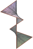
The set of critical points of the argument map restricted to given by the parametrization is the image by of the real part of translated by in as a multiplicative group. So, the set of critical values consists of the translation by of points in the real torus from the real points corresponding to the arguments of the quadrants of . The closure of the coamoeba of contains an arrangement of geodesic circles. Each circle corresponds to an end of the line (i.e., where meets a coordinate axis). The union of these circles is the set of accumulation points of arguments of sequences in with unbounded logarithm, and is called the phase limit set of (see [17] for more details). It is the counterpart of the logarithmic limit set introduced by Bergman in 1971 (see [1] and [7] for more details), which consists of points is our case. In Figure 1 (respectively Figure 2), we draw the amoeba and the coamoeba of a real (respectively non real) line in . The coamoebas in Figure 1, and Figure 2 are made with collaboration with F. Sottile.



5. Volume of (co)amoebas of -dimensional very affine linear spaces in
It was shown by Rullgård and the second author in [19] that the area of the amoeba of a complex algebraic plane curve is always finite, and the bound is given in terms of the area of the Newton polygon of the defining polynomial. Mikhalkin and Rullgård proved that this bound is always sharp for (possibly singular) Harnack curves (see [14]). It was shown by Madani and the first author in [8] that the volume of the amoeba of a -dimensional algebraic variety in with is finite. This generalizes the result of Rullgård and the second author about the finiteness of the volume of the amoeba of plane curves. In this section, we compute the volume of the amoeba of a generic real -dimensional very affine linear space in . We will proceed as follows: (i) We show that the argument map restricted to the subset of regular points in the very affine linear space is injective; (ii) We compute the volume of the coamoeba of any -dimensional very affine linear space in ; (iii) We compute the cardinality of the inverse image under the logarithmic map of any regular value in the amoeba of a real affine space, and prove that this cardinality is a constant and equal to ; (iv) We use that the map conserves the volume i.e., the determinant of its Jacobian has absolute value equal one (see Proposition 3.1 in [9]), and finally we compute the volume of the amoeba, which is equal to the coamoeba volume divided by if the plane is real. We will use the following lemma proved in [10], which is a generalization of Mikhalkin’s Lemma 4.3 in [12] for hypersurface:
Lemma 5.1 (Madani-Nisse).
Let be a dimensional algebraic variety, and be a smooth point of . Then is a critical point for the map if and only if the image of the tangent space to at by the derivative of the complex logarithm contains at least purely imaginary linearly independent vectors with .
Also, we will use the following proposition proved in [10]:
Proposition 5.2 (Madani-Nisse).
Let be a generic -dimensional very affine linear space with . Suppose that the complex dimension of is equal to , with . Then, for any regular value in the amoeba of , the cardinality of is at least .
Let be a generic -dimensional very affine linear space. Suppose is given by the parametrization :
| (4) |
with , where , and are complex numbers for and . Since the space is generic, then there is no .
Definition 5.3.
A generic -dimensional very affine linear space given by the parametrization is said to be real up to a translation by a complex vector in the multiplicative group if and only if the -matrix given by
has rank and all of its entries are real.
Let be the real subgroup of the multiplicative group , and be the finite real subgroup of . For each , let be the parametrization given by where for any , and . Let be the -dimensional very affine linear space in parametrized by . Let us denote by the set of regular values of . Remark that if denotes the identity element of the group , then .
Let and denote by the set of regular values of the coamoeba .
Proposition 5.4.
With the above notations, the following statements hold:
- (i)
For all , the argument map from the subset of regular points of to the set of regular values of its coamoeba is injective;
- (ii)
Let and in with , then the set
is empty;
- (iii)
The union is an open dense subset of the real torus .
First of all, we denote by the coordinates of . So, if is a point in , then and for . Let be a point in the set of regular values of . This means that the linear system of equations and variables in :
with , has a solution in . Moreover, if is viewed as a subgroup of the real torus , then means that the system has a solution in .
Since the matrix defined by:
is the image under the logarithmic Gauss map of the point in , and the matrix has rank when is a regular point.
Claim I. If denotes the matrix conjugate to , then for any regular point of the matrix is of rank .
Proof.
In fact, the rows of the matrix form a basis of the orthogonal space to at the point . So, if the rank of is less than , then the orthogonal space to at contains at least one real vector different than zero. This is equivalent to saying that the tangent space to at contains at least one purely imaginary vector. Indeed, since is a vector different than zero orthogonal to both and , then must be of dimension at least one. By Lemma 5.1, this implies that is a critical point for the logarithmic map, which is in contradiction with our assumption on . ∎
The matrix defining the system is where is
We can check that the rank of is the same as the rank of the matrix with , because the variables and are non zero for all .
Claim II. The rank of the matrix is equal to .
Proof.
Suppose we have a non trivial linear combination of the rows of the matrix that is equal to zero. Hence, there exist a real numbers , and not all equal to zero, with such that:
We get:
Since the matrix is of rank by Claim I, this implies that , and for all . This means that all the ’s and the ’s vanish. This contradict the fact that some of the real numbers ’s and ’s are different than zero by hypothesis. Hence, the real rank of the matrix is equal to . ∎
Proof of Proposition 5.4. Since the -dimensional linear space is generic, the coefficients are different than zero, and the system is consistent. Claim II shows that the system has a unique solution for any in the set of regular values of , which proves the first and the second statements of the proposition. The third statement comes from the fact that the set of for which the determinant of vanishes is a hypersurface in the real torus and then its -volume is zero. In other words, the union is an open dense subset of the real torus .
Corollary 5.5.
The volume of the coamoeba of any generic -dimensional linear space in is equal to .
Proof.
By Proposition 5.4 (iii), the volume of the disjoint union
is equal to the volume of all the real torus . Moreover, they have the same volume, because they are obtained from each other by translation (i.e., isometry of the real torus equipped with the flat metric). So, the volume of one of them must be equal to . ∎
We compute the cardinality of the inverse image under the logarithmic map of any regular value in the amoeba of a generic -dimensional real very affine linear space .
Proposition 5.6.
Let be a generic real affine -dimentional linear subspace of , and be a regular value of its amoeba. Then, the cardinality of is equal .
Proof.
We assume that is given by a parametrization as in , where all the coefficients are real numbers. The matrix defined by:
is invertible, otherwise the image of is a linear space of dimension strictly less than . The following diagram is commutative:
where is the parametrization given by:
Each regular value of the amoeba of the -dimensional linear space is covered times under the logarithmic mapping. Indeed, is a product of lines in . The matrix is real, so the image of the set of critical points of the logarithmic mapping restricted to is the set of critical points of the logarithmic mapping restricted to . By Lemma 5.1, if is a critical in , then the tangent space to at contains at least one purely imaginary vector . Since is real, then the image of in the tangent space to at is also purely imaginary tangent vector, and then, the point is critical. Let and be the set of critical points of the restriction of the logarithmic map to and respectively. Since the volume of their amoebas is finite (see [8]), this means that the set of critical values in their amoebas contains a subset of dimension (at least the topological boundary of the amoeba). Hence, the number of connected components of is equal to the number of connected components of . The fact that the set of critical points of the argument and the logarithmic maps coincide (see e.g., [9]), and by Proposition 5.4, the restriction of the argument map to the set of regular points is injective, then, the cardinality of is at most . Since is real, then by Proposition 5.2, for any regular value , the cardinality of is at least . Hence, the cardinality of the inverse image of a regular value is equal to . ∎
Proof of Theorem 1.2. The first statement of Theorem 1.2 is Corollary 5.5. The second statement of Theorem 1.2 is because the cardinality of the inverse image of a regular value in the amoeba is constant and equal to , and the map conserve the volume (see [9], Proposition 3,1). Hence, the volume of the amoeba in this case is equal to the volume of the coamoeba divided by .
References
- [1] G. M. Bergman, The logarithmic limit-set of an algebraic variety, Trans. Amer. Math. Soc. 157 (1971), 459–469.
- [2] M. Forsberg, M. Passare, and A. Tsikh, Laurent determinants and arrangements of hyperplane amoebas, Advances in Math. 151 (2000), 45–70.
- [3] I. M. Gelfand, M. M. Kapranov and A. V. Zelevinski, Discriminants, resultants and multidimensional determinants, Birkhäuser Boston 1994.
- [4] P. Johansson, Coamoebas, Licentiate Thesis, Stockholm University, 2010.
- [5] M. M. Kapranov, A characterization of A-discriminantal hypersurfaces in terms of the logarithmic Gauss map, Math. Ann. 290, (1991), no. 2, 277–285.
- [6] I. Itenberg, G. Mikhalkin E. Shustin, Tropical Algebraic Geometry, Oberwolfach Seminars, Volume 35, Birkhäuser Basel-Boston-Berlin 2007.
- [7] D. Maclagan and B. Sturmfels, Introduction to tropical geometry. Graduate Studies in Math., Vol 161, American Math. Soc. (2015).
- [8] F. Madani and M. Nisse, On the volume of complex amoebas, Proceedings of the AMS, 141 (2013), 1113–1123.
- [9] F. Madani and M. Nisse, Analytic varieties with finite volume amoebas are algebraic, J. reine angew. Math. Vol. 706, (2015), 67–81.
- [10] F. Madani and M. Nisse, Generalized logarithmic Gauss map and its relation to (co)amoebas, Math. Nachr. 286, No. 14–15, (2013), 1510–1513.
- [11] G. Mikhalkin, Real algebraic curves, moment map and amoebas, Ann.of Math. 151 (2000), 309-326.
- [12] G. Mikhalkin, Decomposition into pairs-of-pants for complex algebraic hypersurfaces,Topology 43 (2004), 1035-1065.
- [13] G. Mikhalkin, Enumerative Tropical Algebraic Geometry In , J. Amer. Math. Soc. 18, (2005), 313-377.
- [14] G. Mikhalkin and H. Rullgård, Amoebas of maximal area, Int. Math. Res. Notices 9, (2001), 441-451.
- [15] M. Nisse, Sur la Géométrie et la Topologie des Amibes et Coamibes des Variétés Algébriques Complexes, Thèse de Doctorat de l’université Pierre et Marie Curie - Paris 6, 2010.
- [16] M. Nisse, Geometric and Combinatorial Structure of Hypersurface Coamoebas, preprint, arXiv:0906.2729.
- [17] M. Nisse and F. Sottile, The phase limit set of a variety, Algebra & Number Theory, 7-2, (2013), 339–352.
- [18] M. Nisse and F. Sottile, Non-Archimedean coAmoebae, Contemporary Mathematics of the AMS Vol. 605, (2013), 73–91.
- [19] M. Passare and H. Rullgård, Amoebas, Monge-Ampère measures and triangulations of the Newton polytope, Duke Math. J. 121, (2004), 481-507.
- [20] K. Purbhoo, A Nullstellensatz for amoebas, Duke Math. J. 141, (2008) no. 3, 407-445.