跳到论文正文
W Papers独立论文阅读器 arXiv:1205.2789 论文正文 计算阅读时间 · 0%
引用这篇论文根据当前论文元数据生成,正式投稿前建议核对。


License: arXiv.org perpetual non-exclusive license
arXiv:1205.2789v2 [math-ph] 04 Jan 2014

Evolution of correlation functions in the hard sphere dynamics

Sergio Simonella Thanks: This work is a revised version of part of the author’s PhD thesis [12], written at the University of Rome “La Sapienza” under the direction of G. Gallavotti. Affiliation: INdAM–COFUND Marie Curie Fellow,
Zentrum Mathematik, TU München,
Boltzmannstrasse 3, 85748 Garching, Germany
Abstract

The series expansion for the evolution of the correlation functions of a finite system of hard spheres is derived from direct integration of the solution of the Liouville equation, with minimal regularity assumptions on the density of the initial measure. The usual BBGKY hierarchy of equations is then recovered. A graphical language based on the notion of collision history originally introduced by Spohn is developed, as a useful tool for the description of the expansion and of the elimination of degrees of freedom.

1 Introduction

In his famous derivation of the Boltzmann equation [8], O. E. Lanford makes use of a series expansion for the time–evolved correlation functions of a classical finite system of hard spheres in a box. This expresses the n−n-point correlation function at time tt as a sum of integral terms involving all the higher order correlation functions at time zero. The expansion is derived, though not rigorously, from iteration of the BBGKY hierarchy of integro–differential equations, and is considered as a “series solution” of its Cauchy problem. A rigorous validation of the hierarchy (formally deduced first by Cercignani in [2]) and of the series has been given years later by H. Spohn in an unpublished note [13], and by R. Illner and M. Pulvirenti in [6] (see also the book [3]), using different methods.

In both the previous papers an assumption on the initial measure is made to derive the BBGKY hierarchy, that is the continuity along trajectories of the hard spheres flow. However, there is no physical reason to expect such a regularity property to hold, and it is worthwhile to notice that the final series expansion makes perfectly sense without assuming it. In fact, Spohn observes at the end of his note, by a density argument, that the expansion can be extended to a more general class of measures having no continuity properties. On the other hand, the interpretation of the BBGKY hierarchy as a family of partial differential equations is not at all easy, nor standard in any case, since it relies on the nontrivial properties of the operator TtT_{t} of the hard sphere dynamics. Hence, the series solution concept appears to be more appropriate for the description of the dynamics in terms of probability distributions, and one wonders whether it is possible to derive it without going through the usual hierarchy. The present paper is devoted to a derivation of the series expansion for the correlation functions, which is not based on the iteration of the BBGKY equations, and never requires continuity along trajectories. We rather construct a method of direct integration of the solution of the Liouville equation, that allows to establish the validity of the expansion in a sense even stronger than those obtained in the existing literature: the result holds for all times in a fixed full measure invariant subset of the phase space, exactly as it happens for the existence of the dynamics of the underlying system of particles. The hierarchy of integro–differential equations is then recovered by resummation of the series, without additional assumptions on the initial measure, thus strengthening an analogous result in [6].

Other rigorous discussions on the hard sphere dynamics and the associated BBGKY hierarchy are given in [15], [5], [10], [11] and [4].

Let us recall the derivation of Lanford and state our main result in an informal way. Consider the vector of correlation functions 𝝆={ρn}n≥1{\bm{\rho}}=\{\rho_{n}\}_{n\geq 1}, where ρn\rho_{n} is defined over the phase space of nn hard spheres of mass mm and diameter a>0a>0 in a box Λ\Lambda. A point in this space is an n−n-tuple (z1,⋯,zn),zj=(qj,pj)(z_{1},\cdots,z_{n}),z_{j}=(q_{j},p_{j}), specifying position and momentum of the nn particles. If NN is the total number of particles, we set ρn=0\rho_{n}=0 for n>Nn>N. Then the BBGKY hierarchy for the evolution of ρ\rho can be written

∂∂t​𝝆​(t)=H​𝝆​(t)+Q​𝝆​(t),\frac{\partial}{\partial t}{\bm{\rho}}(t)=H{\bm{\rho}}(t)+Q{\bm{\rho}}(t)\;, (1.1)

where

(H​𝝆)n​(z1,⋯,zn,t)≡{Hn,ρn}​(z1,⋯,zn,t)\left(H{\bm{\rho}}\right)_{n}(z_{1},\cdots,z_{n},t)\equiv\Big\{H_{n},\rho_{n}\Big\}(z_{1},\cdots,z_{n},t) (1.2)

is the n−n-particles Liouville operator acting on ρn\rho_{n} (including the effects of elastic collisions) and the collision operator is defined by

(Q​𝝆)n​(z1,⋯,zn,t)=a2​∑j=1n∫d​p^​𝑑ω​ω⋅(p^−pjm)​ρn+1​(z1,⋯,zn,qj+a​ω,p^,t).\left(Q{\bm{\rho}}\right)_{n}(z_{1},\cdots,z_{n},t)=a^{2}\sum_{j=1}^{n}\int d\hat{p}\ d\omega\ \omega\cdot\left(\frac{\hat{p}-p_{j}}{m}\right)\rho_{n+1}(z_{1},\cdots,z_{n},q_{j}+a\omega,\hat{p},t)\;. (1.3)

Here p^\hat{p} is integrated over all ℝ3{\mathbb{R}}^{3}, and ω\omega runs over the unit sphere.

If t⟶Tt​(z1,⋯,zn)t\longrightarrow T_{t}(z_{1},\cdots,z_{n}) is the flow of the dynamics, define the translation along trajectories of a vector of functions 𝒇={fn}n≥1{\bm{f}}=\{f_{n}\}_{n\geq 1} as

(S⁡(t)​𝒇)n​(z1,⋯,zn)=fn​(T−t​(z1,⋯,zn)).\left(S(t){\bm{f}}\right)_{n}(z_{1},\cdots,z_{n})=f_{n}(T_{-t}(z_{1},\cdots,z_{n}))\;. (1.4)

Then, integration and iteration of Equation (1.1) leads to the formal solution

𝝆(t)=S(t)𝝆(0)+∑m=1∞∫0tdt1∫0t1dt2⋯∫0tm−1dtmS(t−t1)QS(t1−t2)⋯QS(tm)𝝆(0).{\bm{\rho}}(t)=S(t){\bm{\rho}}(0)+\sum_{m=1}^{\infty}\int_{0}^{t}dt_{1}\int_{0}^{t_{1}}dt_{2}\cdots\int_{0}^{t_{m-1}}dt_{m}S(t-t_{1})QS(t_{1}-t_{2})\cdots QS(t_{m}){\bm{\rho}}(0)\;. (1.5)

In this paper we analyze in detail the structure of Eq. (1.5) and prove that it holds, for all times in a full measure subset of the phase space, for any absolutely continuous measure with density symmetric in the particle labels, and bounded by an equilibrium–like distribution. The hierarchy (1.1) can be obtained then, in the mild sense of [6], by taking the derivative. No assumption of continuity is needed even for this last operation. We also allow the total number of particles NN to be non fixed by the initial measure. The boundedness requirement is stronger than the necessary, and it is the same used by Lanford to control the convergence of the series in the Boltzmann–Grad limit. Here it is made to control easily through all the steps the integrals over momenta of the type (1.3), (1.5).

The main interest of the discussion is the method of the proof. For n=Nn=N Eq. (1.5) reduces to the evolution of the density function, that is the solution of the Liouville equation:

ρN​(z1,⋯,zN,t)=ρN​(T−t​(z1,⋯,zN),0).\rho_{N}(z_{1},\cdots,z_{N},t)=\rho_{N}(T_{-t}(z_{1},\cdots,z_{N}),0)\;. (1.6)

It is desirable that we can construct the series expansion for the ρn\rho_{n} from direct integration of (1.6) over all the phase space of N−nN-n particles compatible with a fixed state (z1,⋯,zn)(z_{1},\cdots,z_{n}). We show that in fact this can be done by eliminating the degrees of freedom particle by particle. To achieve the integration of the single particle state, it is important to understand the structure of the right hand side in (1.5). This has been widely studied since the work of Lanford [8], see for instance [7] or [14]. It results that the integrand function in the generic term of the formula, depends on the states assumed by certain clusters of particles following a fictitious evolution: this is constructed from the state (z1,⋯,zn)(z_{1},\cdots,z_{n}) at time tt, by suitably adding more and more particles as the time flows backwards. Following [14], we shall call collision history such an evolution.

The collision histories can be represented graphically in terms of special binary tree graphs. Therefore, a graphical picture of the series expansion (1.5) is obtained. This representation is our basic tool. In fact, it turns out that the integration of a particle state itself can be translated in graphical language, through appropriate operations over tree graphs. The graphical rules corresponding to the elimination of a particle state, clarify how the various terms of the expansion for ρn\rho_{n} emerge from those for ρn+1\rho_{n+1}, thus considerably simplifying the presentation of the proof. The analytical operations corresponding to these rules, are nothing but a suitable partitioning of the integration domain, and convenient representation (change of variables) of the subsets of the partition. Nevertheless, in order to establish the graphical rules, it is also essential to prove that some classes of collision histories give a net null contribution to the integration of the particle state: this is done again with the help of the tree graphs, by showing explicit one by one cancellations among the collision histories of these classes.

The paper is organised as follows. In Section 2 we define the model, we introduce our notations and state our assumptions on the initial measure. In Section 3 we introduce the concept of collision history, as well as the graphical rules for its representation, and explain how to represent formula (1.5) in terms of the tree graphs. In Section 4 we present our main results, while in Section 5 we discuss the proof of the main theorem, establishing the above mentioned graphical integration rules, and applying them to the generic inductive step. In Section 6 we present the conclusions. A discussion on the hard sphere dynamics is deferred to the Appendix.

2 The hard sphere system

In this section we set model and notations, which we inherit essentially from [13], and state some preliminary result on the hard sphere dynamics (Section 2.1). In Section 2.2 we introduce the class of measures on which we will work.

2.1 Model and notations

Let us consider a system of NN hard spheres of unit mass and of diameter a>0a>0 moving in a box Λ⊂ℝ3\Lambda\subset{\mathbb{R}}^{3}. Λ\Lambda is bounded open and has a piecewise smooth elastically reflecting boundary ∂Λ\partial\Lambda. We will denote zi=(qi,pi)∈Λ×ℝ3z_{i}=(q_{i},p_{i})\in\Lambda\times{\mathbb{R}}^{3} the configuration of the ii–th particle, i=1,⋯,Ni=1,\cdots,N. For groups of particles we will use the short notations 𝒛n=z1,⋯,zn,{\bm{z}}_{n}=z_{1},\cdots,z_{n}, 𝒛n,j=zn+1,⋯,zn+j{\bm{z}}_{n,j}=z_{n+1},\cdots,z_{n+j}. When there is no risk of confusion, we will simply call “particle ii” a particle whose configuration is labelled by an index ii.

We introduce the nn particle phase space, n=1,⋯,Nn=1,\cdots,N,

Γn={𝒛n∈(Λ×ℝ3)n||qi−q|≥a/2 for every q∈∂Λand |qi−qj|≥a,i≠j}.\Gamma_{n}=\Big\{{\bm{z}}_{n}\in(\Lambda\times{\mathbb{R}}^{3})^{n}\ \Big|\ |q_{i}-q|\geq a/2\mbox{ for every }q\in\partial\Lambda\ \mbox{and\ }|q_{i}-q_{j}|\geq a,\ i\neq j\Big\}\;. (2.1)

A state of the system is given by a point in the full phase space ΓN\Gamma_{N}.

The equations of motion for the nn particle system are defined as follows. Between collisions each particle moves on a straight line maintaining unchanged its velocity. In a collision of two hard spheres at positions qi,qjq_{i},q_{j} with ω=(qi−qj)/|qi−qj|=(qi−qj)/a∈S2\omega=(q_{i}-q_{j})/|q_{i}-q_{j}|=(q_{i}-q_{j})/a\in S^{2} and with incoming momenta pi′,pj′p^{\prime}_{i},p^{\prime}_{j} (that means (pi′−pj′)⋅ω<0(p^{\prime}_{i}-p^{\prime}_{j})\cdot\omega<0), we have instantaneous transformation to the outgoing momenta pi,pjp_{i},p_{j} (with (pi−pj)⋅ω>0(p_{i}-p_{j})\cdot\omega>0) given by

pi=pi′−ω⁡[ω⋅(pi′−pj′)],\displaystyle p_{i}=p^{\prime}_{i}-\omega[\omega\cdot(p^{\prime}_{i}-p^{\prime}_{j})]\;,
pj=pj′+ω⁡[ω⋅(pi′−pj′)].\displaystyle p_{j}=p^{\prime}_{j}+\omega[\omega\cdot(p^{\prime}_{i}-p^{\prime}_{j})]\;. (2.2)

Finally, in a collision of a particle with momentum pi′p^{\prime}_{i} with the wall ∂Λ\partial\Lambda at a point qq which is regular (there is only one point of contact between the wall and the sphere, and the normal to the surface at that point is well defined), we have instantaneous transformation to the reflected outgoing momentum pip_{i} given by

pi=pi′−2​n​(q)​(n⁡(q)⋅pi′),\displaystyle p_{i}=p^{\prime}_{i}-2n(q)(n(q)\cdot p^{\prime}_{i})\;, (2.3)

where n⁡(q)n(q) is the inner unit vector normal to ∂Λ\partial\Lambda in q.q. It is easy to see that the collision transformations (2.2) and (2.3) are invertible and preserve Lebesgue measure on ℝ3×ℝ3{\mathbb{R}}^{3}\times{\mathbb{R}}^{3} and ℝ3{\mathbb{R}}^{3} respectively.

The above prescription for the equations of motion does not cover all possible situations, e.g. triple collisions and collisions with corner points of the walls are excluded. Nevertheless, we have the following basic result:

Proposition 1.

[Existence of the dynamics (I)] In Γn\Gamma_{n} there is a subset Γn∗,\Gamma_{n}^{*}, whose complement is a Lebesgue null set, such that for any 𝐳n∈Γn∗{\bm{z}}_{n}\in\Gamma_{n}^{*} there is a unique mapping

t↦Tt(n)​𝒛n∈Γn∗t∈ℝt\mapsto T_{t}^{(n)}{\bm{z}}_{n}\in\Gamma_{n}^{*}\ \ \ \ \ \ \ \ \ \ t\in{\mathbb{R}} (2.4)

which is a solution of the equations of motion having T0(n)​𝐳n=𝐳n.T_{0}^{(n)}{\bm{z}}_{n}={\bm{z}}_{n}. Moreover, the shifts along trajectories 𝐳n↦Tt(n)​𝐳n{\bm{z}}_{n}\mapsto T_{t}^{(n)}{\bm{z}}_{n} define a one–parameter group of Borel maps on Γn\Gamma_{n} which leave Lebesgue measure invariant.

This has been stated and proved by Alexander in [1], pages 18–29, and it holds under few simple regularity assumptions on ∂Λ\partial\Lambda (see pages 13–14 of [1] for the details on ∂Λ\partial\Lambda). We shall make the same assumptions in the present paper. The set Γn∗\Gamma_{n}^{*} is shown to be a countable intersection of open sets with full measure. The operator (2.4) is called the flow of the nn particle dynamics. Another analysis of the hard sphere dynamics may be found in [9], [3].

Observe that (unlike in [1]) we do not identify ingoing and outgoing momenta of a collision, but we regard them as corresponding to distinct points in phase space, so that the flow Tt(n)T^{(n)}_{t} is only piecewise continuous in tt. When necessary, we distinguish the limit from the future (+)(+) and the limit from the past (−)(-) writing

Tt±(n)​𝒛n=limε→0+Tt±ε(n)​𝒛n.T^{(n)}_{t\pm}{\bm{z}}_{n}=\lim_{\varepsilon\rightarrow 0^{+}}T^{(n)}_{t\pm\varepsilon}{\bm{z}}_{n}\;. (2.5)

For instance, in the statement of Proposition 1, when 𝒛n∈Γn∗∩∂Γn,{\bm{z}}_{n}\in\Gamma_{n}^{*}\cap\partial\Gamma_{n}, it is understood that either T0+(n)​𝒛n=𝒛nT_{0+}^{(n)}{\bm{z}}_{n}={\bm{z}}_{n} or T0−(n)​𝒛n=𝒛n.T_{0-}^{(n)}{\bm{z}}_{n}={\bm{z}}_{n}. From now on, to be more definite we fix the (irrelevant) convention

Tt(n)​𝒛n=Tt+(n)​𝒛n.T_{t}^{(n)}{\bm{z}}_{n}=T_{t+}^{(n)}{\bm{z}}_{n}\;. (2.6)

The complement of Γn∗\Gamma_{n}^{*} in Γn\Gamma_{n} can be identified with the subset of points of Γn\Gamma_{n} that evolved in time run into either:

  • •

    a “multiple” collision, that is (i) simultaneous contact of more than two hard spheres, (ii) simultaneous contact of two hard spheres with each other and at the same time with ∂Λ\partial\Lambda or (iii) simultaneous contact of one hard sphere with two different points of ∂Λ\partial\Lambda;

  • •

    a grazing collision with the wall (n⁡(q)⋅pi′=0n(q)\cdot p^{\prime}_{i}=0) or a grazing two–body collision ((pi′−pj′)⋅ω=0(p^{\prime}_{i}-p^{\prime}_{j})\cdot\omega=0);

  • •

    a collision of a particle with a singular point q∈∂Λq\in\partial\Lambda where the normal vector n⁡(q)n(q) is not well defined;

  • •

    infinitely many collisions in finite time.

The flow through such situations will not be specified. We shall refer to them as the “singular configurations” (some examples in which a particle undergoes infinitely many collisions in a finite time are given in Sec. II.C of [1]).

We list some more notations that will be useful along the whole paper. For 𝒛n∈Γn,{\bm{z}}_{n}\in\Gamma_{n}, we set

Γk​(𝒛n)={𝒚k∈(Λ×ℝ3)k|(𝒛n,𝒚k)∈Γn+k},\displaystyle\Gamma_{k}({\bm{z}}_{n})=\Big\{{\bm{y}}_{k}\in(\Lambda\times{\mathbb{R}}^{3})^{k}\ \Big|\ ({\bm{z}}_{n},{\bm{y}}_{k})\in\Gamma_{n+k}\Big\}\;,
Ωi(𝒛n)={ω∈S2|(𝒛n,qi+aω,p)∈Γn+1∀p∈ℝ3},i=1,⋯,n.\displaystyle\Omega_{i}({\bm{z}}_{n})=\Big\{\omega\in S^{2}\ \Big|\ ({\bm{z}}_{n},q_{i}+a\omega,p)\in\Gamma_{n+1}\ \ \forall p\in{\mathbb{R}}^{3}\Big\}\;,\ \ \ \ \ \ \ \ \ \ \ i=1,\cdots,n\;. (2.7)

To conclude this section, we pursue a bit further the analysis on the dynamics of the system of particles. The following result will be used to study the properties of correlation functions:

Proposition 2.

[Existence of the dynamics (II)] In Γn\Gamma_{n} there is a subset Γn†,\Gamma_{n}^{\dagger}, whose complement is a Lebesgue null set, such that Γn†⊆Γn∗,\Gamma_{n}^{\dagger}\subseteq\Gamma_{n}^{*}, Tt(n)​Γn†=Γn†T^{(n)}_{t}\Gamma_{n}^{\dagger}=\Gamma_{n}^{\dagger} and, for k=1,⋯,N−n,k=1,\cdots,N-n,

𝒛n∈Γn†⇒(𝒛n,𝒛n,k)∈Γn+k∗​ for a.a. 𝒛n,k∈Γk​(𝒛n).{\bm{z}}_{n}\in\Gamma_{n}^{\dagger}\ \Rightarrow\ ({\bm{z}}_{n},{\bm{z}}_{n,k})\in\Gamma_{n+k}^{*}\mbox{\ for a.a. ${\bm{z}}_{n,k}\in\Gamma_{k}({\bm{z}}_{n})$}\;. (2.8)

This statement is a consequence of Proposition 1. Its proof is given in the Appendix. Notice that 𝒛n∈Γn†{\bm{z}}_{n}\in\Gamma_{n}^{\dagger} implies also 𝒛n+k∈Γn+k†{\bm{z}}_{n+k}\in\Gamma_{n+k}^{\dagger} for a.a. 𝒛n,k{\bm{z}}_{n,k}. The set Γn†\Gamma_{n}^{\dagger} can be identified with

Γn†={𝒛n∈Γn∗|(Ts(n)​𝒛n,𝒛n,k)∈Γn+k∗​∀s​ and a.a. ​𝒛n,k∈Γk​(Ts(n)​𝒛n)},\Gamma_{n}^{\dagger}=\Big\{{\bm{z}}_{n}\in\Gamma_{n}^{*}\ \Big|\ (T^{(n)}_{s}{\bm{z}}_{n},{\bm{z}}_{n,k})\in\Gamma_{n+k}^{*}\ \forall s\mbox{ and a.a. }{\bm{z}}_{n,k}\in\Gamma_{k}(T^{(n)}_{s}{\bm{z}}_{n})\Big\}\;, (2.9)

which is also the maximal subset obeying the properties of Proposition 2.

2.2 Measures over the phase space

Since all the particles of the system are identical, we will work with the space ℒN\mathcal{L}_{N} of Borel measurable functions fN:ΓN→ℝf_{N}:\Gamma_{N}\rightarrow{\mathbb{R}}, symmetric in the particle labels (fN​(Π⁡(z1,…,zN))=fN​(z1,…,zN)f_{N}(\Pi(z_{1},\dots,z_{N}))=f_{N}(z_{1},\dots,z_{N}) for any permutation Π\Pi). We also assume that the functions in ℒN\mathcal{L}_{N} have a boundedness property on ΓN\Gamma_{N} of the type

|fN​(𝒛N)|≤A​∏j=1Nhβ​(pj),hβ​(p)=(β2​π)32​e−β2​p2,|f_{N}({\bm{z}}_{N})|\leq A\prod_{j=1}^{N}h_{\beta}(p_{j})\;,\ \ \ \ \ \ \ \ \ \ \ \ \ \ \ h_{\beta}(p)=\left(\frac{\beta}{2\pi}\right)^{\frac{3}{2}}e^{-\frac{\beta}{2}p^{2}}\;, (2.10)

for some A,β>0A,\beta>0.

In Eq. (2.10) we ignore the (possible) dependence on NN of the constant AA, being the total number of particles always fixed throughout the paper. In particular, we allow AA to grow exponentially with NN. It is worth to notice that this includes the states considered in the derivation of the Boltzmann equation [8].

Suppose to have an initial measure PP on ΓN\Gamma_{N} with density fN0∈ℒNf_{N}^{0}\in\mathcal{L}_{N} with respect to the Lebesgue measure d​𝒛N=d​z1​…​d​zNd{\bm{z}}_{N}=dz_{1}\dots dz_{N},

P⁡(d​𝒛N)=fN0​(𝒛N)​d​𝒛N.\displaystyle P(d{\bm{z}}_{N})=f_{N}^{0}({\bm{z}}_{N})d{\bm{z}}_{N}\;. (2.11)

Then, because the flow Tt(N)T^{(N)}_{t} preserves the Lebesgue measure, the evolved measure at time tt has a density fN​(t)f_{N}(t) given by

fN​(𝒛N,t)=fN0​(T−t(N)​𝒛N)f_{N}({\bm{z}}_{N},t)=f_{N}^{0}(T^{(N)}_{-t}{\bm{z}}_{N}) (2.12)

almost everywhere in ΓN\Gamma_{N}, which is the Liouville equation in mild form. Points of ΓN∖ΓN∗\Gamma_{N}\setminus\Gamma_{N}^{*} are removed from (2.12). Notice that estimate (2.10) is preserved in the time evolution by conservation of energy. In particular, fN​(t)∈ℒNf_{N}(t)\in\mathcal{L}_{N}. Of course since the flow Tt(N)T^{(N)}_{t} is only well defined almost surely, even densities that are smooth at time zero will only be ℒN−\mathcal{L}_{N}-functions at time tt. Observe that, by our convention (2.6), fNf_{N} takes the same value in incoming and outgoing states of collision (a property not to be confused with the continuity along trajectories; see Eq. (4.1) below).

We define the correlation functions ρn(t)∈ℒn,n=1,2,…\rho_{n}(t)\in\mathcal{L}_{n},n=1,2,\dots by

ρn​(𝒛n,t)=N​…​(N−n+1)​∫ΓN−n​(𝒛n)d​zn+1​…​d​zN​fN​(𝒛N,t),n≤N,\displaystyle\rho_{n}({\bm{z}}_{n},t)=N\dots(N-n+1)\int_{\Gamma_{N-n}({\bm{z}}_{n})}dz_{n+1}\dots dz_{N}f_{N}({\bm{z}}_{N},t)\;,\ \ \ \ \ n\leq N\;,
ρn=0,n>N,\displaystyle\rho_{n}=0\;,\ \ \ \ \ \ \ \ \ \ n>N\;,
ρn0​(𝒛n)≡ρn​(𝒛n,0).\displaystyle\rho_{n}^{0}({\bm{z}}_{n})\equiv\rho_{n}({\bm{z}}_{n},0)\;. (2.13)

PP can be, in general, any signed measure with density in ℒN.{\cal L}_{N}. In the case PP is a probability measure, the quantity

1N⋯(N−n+1)∫𝒲dz1⋯dznρn(z1,⋯,zn,t)\frac{1}{N\cdots(N-n+1)}\int_{\cal W}dz_{1}\cdots dz_{n}\rho_{n}(z_{1},\cdots,z_{n},t) (2.14)

is the probability of finding particles 1,2,⋯,n1,2,\cdots,n at time tt in the Borel set 𝒲∈Γn{\cal W}\in\Gamma_{n}.

3 Collision histories

In this section we analyze the structure of the expansion on the right hand side of (1.5) (Section 3.1). This is given in general by a large variety of terms. In order to have a clear picture of the many terms of the expansion and of the configurations of particles involved in them, we shall establish rules for their graphical representation (Section 3.2).

From now on, without loss of generality and to avoid overweight of notation, the time tt will be always supposed to be positive.

3.1 The structure of formula (1.5): an integral over fictitious evolutions of particles

Let us look carefully at the explicit expression of the right hand side in Eq. (1.5). We compute it, say, in 𝒛n{\bm{z}}_{n}, taking into account the definitions (1.3) and (1.4). We see that, in the generic term, the integrand function contains one time–zero correlation function. This is evaluated in a configuration of particles which can be found by flowing backwards in time the configuration 𝒛n{\bm{z}}_{n}, and suitably adding new particles at the times t1,t2t_{1},t_{2} etcetera. The new particles appear in a collision configuration with one of the pre–existent particles. This describes a special evolution that will be called “collision history”, a name first used by Spohn in [13].

We want to stress since the beginning that the collision history is not a real trajectory of the particle system, and the associated collisions are not a sequence of real collisions. The correspondence between collision histories and sequences of real collisions is only very indirect ([13]).

We begin by explaining how to construct a collision history. The ingredients are the collection of variables (in parentheses we specify what will be their interpretation):

  • •

    n∈{1,2,3,⋯}n\in\{1,2,3,\cdots\} (starting number of particles),

  • •

    m∈{0,1,2,⋯}m\in\{0,1,2,\cdots\} (number of added particles),

  • •

    𝒛n∈Γn∗{\bm{z}}_{n}\in\Gamma_{n}^{*} (starting configuration),

  • •

    t>0t>0 (total time span),

  • •

    𝒕m∈ℝm​(m≥1){\bm{t}}_{m}\in{\mathbb{R}}^{m}\ (m\geq 1)\ with t≡t0>t1>⋯>tm>tm+1≡0t\equiv t_{0}>t_{1}>\cdots>t_{m}>t_{m+1}\equiv 0 (times of creation

    of added particles),

  • •

    𝒋m∈ℕm​(m≥1){\bm{j}}_{m}\in{\mathbb{N}}^{m}\ (m\geq 1)\ with j1∈In,⋯,jm∈In+m−1,j_{1}\in I_{n},\cdots,j_{m}\in I_{n+m-1}, where Ik={1,⋯,k}I_{k}=\{1,\cdots,k\} (progenitors of

    added particles),

  • •

    𝒑^m∈ℝ3​m​(m≥1)\hat{\bm{p}}_{m}\in{\mathbb{R}}^{3m}\ (m\geq 1) (momenta of added particles

    at the time of their creation),

  • •

    𝝎m∈S2​m​(m≥1){\bm{\omega}}_{m}\in S^{2m}\ (m\geq 1)\ , with a constraint defined below (relative position, in units of a,a, of the added

    particles with respect to their progenitors).

To any choice of the variables in the list we associate a backwards evolution. We indicate with the greek letter

ζi​(s)=(ξi​(s),πi​(s))∈Λ×ℝ3\zeta_{i}(s)=(\xi_{i}(s),\pi_{i}(s))\in\Lambda\times{\mathbb{R}}^{3} (3.1)

the configuration of particle ii (position and momentum) at time ss in such evolution, defined as follows. Take the starting configuration 𝒛n∈Γn∗{\bm{z}}_{n}\in\Gamma_{n}^{*}, put (ζ1​(t),⋯,ζn​(t))=𝒛n(\zeta_{1}(t),\cdots,\zeta_{n}(t))={\bm{z}}_{n}, and evolve it backwards in time as if there were no other particles in the space up to time t1.t_{1}. This defines the piecewise continuous trajectory (ζ1​(s),⋯,ζn​(s))(\zeta_{1}(s),\cdots,\zeta_{n}(s)) for t1<s<t,t_{1}<s<t, that is (ζ1​(s),⋯,ζn​(s))=T−t+s(n)​𝒛n.(\zeta_{1}(s),\cdots,\zeta_{n}(s))=T^{(n)}_{-t+s}{\bm{z}}_{n}. Set (ζ1​(t1),⋯,ζn​(t1))=T−t+t1(n)​𝒛n.(\zeta_{1}(t_{1}),\cdots,\zeta_{n}(t_{1}))=T^{(n)}_{-t+t_{1}}{\bm{z}}_{n}. If m=0,m=0, put t1=0:t_{1}=0: the construction is finished. Otherwise, at time t1t_{1} stop your nn particle system and add particle n+1n+1 in a state ζn+1​(t1)=(ξj1​(t1)+a​ω1,p^1),\zeta_{n+1}(t_{1})=(\xi_{j_{1}}(t_{1})+a\omega_{1},\hat{p}_{1}), with ω1∈Ωj1​(𝜻n​(t1))\omega_{1}\in\Omega_{j_{1}}({\bm{\zeta}}_{n}(t_{1})) and such that the dynamics of the obtained system of n+1n+1 particles is well defined, i.e. (𝜻n​(t1),ζn+1​(t1))∈Γn+1∗.({\bm{\zeta}}_{n}(t_{1}),\zeta_{n+1}(t_{1}))\in\Gamma_{n+1}^{*}. Observe that, at fixed 𝒛n,t1,{\bm{z}}_{n},t_{1}, we will have either an incoming or an outgoing collision between particles j1j_{1} and n+1n+1, depending on the chosen values of ω1,p^1\omega_{1},\hat{p}_{1}. Now, evolve backwards in time particles 1,…,n+11,\dots,n+1 as if there were no other particles in the space up to time t2<t1:t_{2}<t_{1}: this defines the piecewise continuous trajectory (ζ1​(s),⋯,ζn+1​(s))=T−t1+s(n+1)​𝜻n+1​(t1)(\zeta_{1}(s),\cdots,\zeta_{n+1}(s))=T^{(n+1)}_{-t_{1}+s}{\bm{\zeta}}_{n+1}(t_{1}) for t2<s<t1.t_{2}<s<t_{1}. Notice that, soon after t1,t_{1}, particle j1j_{1} in the backwards evolution will deviate from its free motion if and only if ω1,p^1\omega_{1},\hat{p}_{1} correspond to an outgoing collision. Set 𝜻n+1​(t2)=T−t1+t2(n+1)​𝜻n+1​(t1).{\bm{\zeta}}_{n+1}(t_{2})=T^{(n+1)}_{-t_{1}+t_{2}}{\bm{\zeta}}_{n+1}(t_{1}). If m=1m=1 (t2=0t_{2}=0) the construction is finished. Otherwise, at time t2t_{2} stop the system and add particle n+2n+2 as above with momentum p^2\hat{p}_{2} and position at distance a​ω2a\omega_{2} from particle j2,j_{2}, with ω2∈Ωj2​(𝜻n+1​(t2))\omega_{2}\in\Omega_{j_{2}}({\bm{\zeta}}_{n+1}(t_{2})) and the constraint that the obtained system of n+2n+2 particles is in Γn+2∗.\Gamma_{n+2}^{*}. Later on evolve your n+2n+2 particles backwards in time up to time t3<t2t_{3}<t_{2}, and so on up to the final step, which is the evolution of particles 1,…,n+m1,\dots,n+m with the flow T−tm+s(n+m),0≤s<tm.T^{(n+m)}_{-t_{m}+s},0\leq s<t_{m}. We shall say in the future that particle n+kn+k is “created” by particle jkj_{k}, or that particle jkj_{k} is its “progenitor”. An example is pictured in 1.

Refer to caption
Figure 1: Trajectory drawn by the particles in a collision history, in the case n=2,j1=2,j2=1n=2,j_{1}=2,j_{2}=1. Here particle 33 is added in an incoming collision configuration (ω1⋅(p^1−πj1​(t1))<0\omega_{1}\cdot(\hat{p}_{1}-\pi_{j_{1}}(t_{1}))<0), while particle 44 is added in an outgoing collision configuration (ω2⋅(p^2−πj2​(t2))>0\omega_{2}\cdot(\hat{p}_{2}-\pi_{j_{2}}(t_{2}))>0).

We will use always greek alphabet for collision histories. We will call 𝜻⁡(s){\bm{\zeta}}(s) the configuration of all the particles of the history at time s.s. When no confusion arises, this symbol will have no subscript specifying the number of particles, which is actually variable in time, so that

𝜻⁡(s)=(𝝃⁡(s),𝒑⁡(s))=(ξ1​(s),⋯,ξn+k​(s),π1​(s),⋯,πn+k​(s))for s∈(tk+1,tk].{\bm{\zeta}}(s)=({\bm{\xi}}(s),{\bm{p}}(s))=(\xi_{1}(s),\cdots,\xi_{n+k}(s),\pi_{1}(s),\cdots,\pi_{n+k}(s))\ \ \ \ \ \ \ \ \ \ \ \mbox{for $s\in(t_{k+1},t_{k}]$}\;. (3.2)

In particular, if ss coincides with a time tkt_{k}, then 𝜻⁡(s){\bm{\zeta}}(s) is the configuration of the particles of the evolution after having added the new particle n+kn+k (but before the related backwards collision, in the case the added particle is in outgoing configuration):

𝜻⁡(tk)=(𝜻n+k−1​(tk),ξjk​(tk)+a​ωk,p^k).{\bm{\zeta}}(t_{k})=({\bm{\zeta}}_{n+k-1}(t_{k}),\xi_{j_{k}}(t_{k})+a\omega_{k},\hat{p}_{k})\;. (3.3)

Now we turn back to the description of the series expansion. A careful look of formula (1.5) leads to the following more explicit formal representation:

ρn​(𝒛n,t)=∑m=0∞∑j1,⋯,jmjk∈In+k−1∫𝒞𝒋m​(𝒛n,t)d​μ​(𝒕m,𝝎m,𝒑^m)​(∏k=1mB⁡(ωk,p^k−πjk​(tk)))​ρn+m0​(𝜻⁡(0))\rho_{n}({\bm{z}}_{n},t)=\sum_{m=0}^{\infty}\sum_{\begin{subarray}{c}j_{1},\cdots,j_{m}\\ j_{k}\in I_{n+k-1}\end{subarray}}\int_{{\cal C}_{{\bm{j}}_{m}}({\bm{z}}_{n},t)}d\mu({\bm{t}}_{m},{\bm{\omega}}_{m},\hat{\bm{p}}_{m})\left(\prod_{k=1}^{m}B(\omega_{k};\hat{p}_{k}-\pi_{j_{k}}(t_{k}))\right)\rho_{n+m}^{0}({\bm{\zeta}}(0)) (3.4)

where

dμ(𝒕m,𝝎m,𝒑^m)≡dμm=dt1⋯dtmdω1⋯dωmdp^1⋯dp^m\displaystyle d\mu({\bm{t}}_{m},{\bm{\omega}}_{m},\hat{\bm{p}}_{m})\equiv d\mu_{m}=dt_{1}\cdots dt_{m}d\omega_{1}\cdots d\omega_{m}d\hat{p}_{1}\cdots d\hat{p}_{m}
(= volume element over ℝm×S2​m×ℝ3​m),\displaystyle\ \ \ \ \ \ \ \ \ \ \ \ \ \ \ \ \ \ \ \ \ \ \ \ \ \ \ \ \ \ \mbox{(= volume element over ${\mathbb{R}}^{m}\times S^{2m}\times{\mathbb{R}}^{3m}$)}\;,
B⁡(ωk,p^k−πjk​(tk))≡Bk=a2​ωk⋅(p^k−πjk​(tk)),\displaystyle B(\omega_{k};\hat{p}_{k}-\pi_{j_{k}}(t_{k}))\equiv B_{k}=a^{2}\omega_{k}\cdot\left(\hat{p}_{k}-\pi_{j_{k}}(t_{k})\right)\;,
𝒞𝒋m(𝒛n,t)={(𝒕m,𝝎m,𝒑^m)∈ℝm×S2​m×ℝ3​m|\displaystyle{\cal C}_{{\bm{j}}_{m}}({\bm{z}}_{n},t)=\Big\{({\bm{t}}_{m},{\bm{\omega}}_{m},\hat{\bm{p}}_{m})\in{\mathbb{R}}^{m}\times S^{2m}\times{\mathbb{R}}^{3m}\ \Big|\
t>t1>⋯>tm>0,ωk∈Ωjk(𝜻n+k−1(tk))}.\displaystyle\ \ \ \ \ \ \ \ \ \ \ \ \ \ \ \ \ \ \ \ t>t_{1}>\cdots>t_{m}>0,\ \omega_{k}\in\Omega_{j_{k}}({\bm{\zeta}}_{n+k-1}(t_{k}))\Big\}\;. (3.5)

The volume element d​μmd\mu_{m} is the induced Lebesgue measure over ℝm×S2​m×ℝ3​m{\mathbb{R}}^{m}\times S^{2m}\times{\mathbb{R}}^{3m}. The sum over mm is extended to infinity by the convention in (2.13). The term m=0m=0 must be interpreted as ρn0​(T−t(n)​𝒛n)\rho_{n}^{0}(T^{(n)}_{-t}{\bm{z}}_{n}).

In the following sections we will rigorously derive (3.4) from Liouville equation, starting with an initial density fN0∈ℒN.f_{N}^{0}\in\mathcal{L}_{N}. In particular, we will check its consistency, and this will require to prove that the collision histories involved in the integrand are well defined d​μm−d\mu_{m}-a.e. in the domain of integration.

Observe that, since ρn+m0\rho_{n+m}^{0} satisfies an estimate as in (2.10), applying conservation of energy at each creation of the collision history we find

ρn+m0​(𝜻⁡(0))≤A′​∏j=1nhβ​(pj)​∏k=1mhβ​(p^k)\rho_{n+m}^{0}({\bm{\zeta}}(0))\leq A^{\prime}\prod_{j=1}^{n}h_{\beta}(p_{j})\prod_{k=1}^{m}h_{\beta}(\hat{p}_{k}) (3.6)

for some A′>0A^{\prime}>0. In particular, once we have proven that (∏kBk)​ρn+m0​(𝜻⁡(0))(\prod_{k}B_{k})\rho_{n+m}^{0}({\bm{\zeta}}(0)) is a well defined measurable function, it follows that its integral in any of the variables 𝒛n,𝒕m,𝝎m,𝒑^m{\bm{z}}_{n},{\bm{t}}_{m},{\bm{\omega}}_{m},\hat{\bm{p}}_{m} is absolutely convergent. We will use this fact repeatedly during the proof of our results.

3.2 A graphical expression of (1.5)

Due to the structure of the collision histories, as described in the previous section, it is quite natural to graphically represent each term in the expansion (3.4) as a binary tree. Let us introduce at a formal level the useful family of graphs.

For fixed nn, we define the m−m-node, n−n-particle tree graph, denoted 𝒯n,m{\cal T}_{n,m}, as the collection of integers j1,⋯,jmj_{1},\cdots,j_{m} appearing in the right hand side of Eq. (3.4), i.e.

j1∈In,j2∈In+1,⋯,jm∈In+m−1,with Ik={1,2,⋯,k},j_{1}\in I_{n},j_{2}\in I_{n+1},\cdots,j_{m}\in I_{n+m-1}\;,\ \ \ \ \ \ \mbox{with\ \ \ \ \ \ $I_{k}=\{1,2,\cdots,k\},$} (3.7)

so that we shall write

∑j1,⋯,jmjk∈In+k−1=∑𝒯n,m.\sum_{\begin{subarray}{c}j_{1},\cdots,j_{m}\\ j_{k}\in I_{n+k-1}\end{subarray}}=\sum_{{\cal T}_{n,m}}\;. (3.8)

This has an equivalent graphical representation, given by the following simple procedure. First, draw nn horizontal lines, all of them with the same length, stacked one above the other. Assign them the numbers 1,2,3,⋯,1,2,3,\cdots, from the bottom upwards. We will refer to such lines as the “root lines” of the tree graph. Time will be thought as flowing from right to left along a horizontal axis, in such a way that the left extremum of the segments corresponds to time tt while the right corresponds to time zero. Now, if m≥1m\geq 1, draw a heavy dot over the line j1j_{1} (so that the line “crosses” the dot) and a new straight line with a certain slope (say, between 00 and π/2\pi/2), having left extremum in the dot and right extremum at time zero. We shall call the dot “node 11” and the new added segment “line n+1n+1”. Node 11 will correspond to a time t1∈(0,t)t_{1}\in(0,t). If m≥2m\geq 2, draw a heavy dot (“node 22”) over the line j2j_{2}, corresponding to a time t2∈(0,t1)t_{2}\in(0,t_{1}) (hence on the right with respect to node 11), and a new straight line (“line 22”) having left extremum in the dot and right extremum at time zero. This new line shall be horizontal if attached (through the node) to a sloped line, and sloped if attached to a horizontal line. Finally, iterate these operations until the last node (“mm”) and the last line (“n+mn+m”) are added. We may agree to avoid intersections between lines. Right extrema of the lines of a tree will be called “endpoints”, while left extrema of the root lines will be called “roots”. An example of tree graph is given in Figure 2.
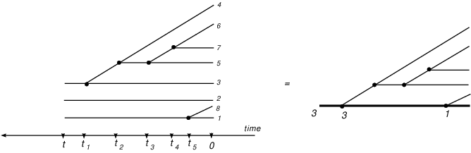
Refer to caption
Figure 2: Tree graph 𝒯3,5=3,4,5,6,1{\cal T}_{3,5}=3,4,5,6,1. On the right, a second equivalent representation.

As shown in the figure, an alternative graphical representation can be given by superposing the nn root lines. In this case the (only) root line of the graph is special: it will be drawn as a bold line and it will be decorated as follows: (i) a label nn is attached to the root; (ii) if node kk lies on the root line, a label jkj_{k} is attached to it. Though the graph in the left hand side of Figure 2 is perhaps more standard, we will sometimes use decorated trees as in the right, in order to avoid large diagrams. Furthermore, to simplify the notation, we will not add to the drawing the axis of time, and we will not indicate explicitly the names of the lines (see the right hand side of Figure 2).

Note that two tree graphs are “equivalent” if they can be superposed, together with their labels and without altering their topological structure neither the ordering of its nodes. In other words, the nodes of a tree are ordered along the time axis, so that the total number of different graphs 𝒯n,m{\cal T}_{n,m} is n(n+1)⋯(n+m−1)n(n+1)\cdots(n+m-1).

Since a collision history is identified by the collection of variables listed on page 3.1, we see that 𝒯n,m{\cal T}_{n,m} can be associated to a class of collision histories. Namely, 𝒯n,m{\cal T}_{n,m} represents all the collision histories with nn particles at time tt and mm particles added during the backwards evolution, with progenitors specified by j1,⋯,jm.j_{1},\cdots,j_{m}. In this sense, we have the dynamical interpretation of graphs:

– root lines: particles 1,⋯,n1,\cdots,n of the history, leaving from time 00 to time t;t;

– line n+k:n+k: particle n+kn+k of the history, leaving from time 00 to time tkt_{k};

– node k:k: binary collision in which particle n+kn+k is created from the progenitor jk.j_{k}.

To have a precise correspondence between single collision histories and graphs it would be sufficient to add to the picture the following decorations: (i) labels z1,⋯,zn,tz_{1},\cdots,z_{n},t attached to the roots of the graph indicating the starting configuration and the time span; (ii) triples (t1,ω1,p^1),⋯,(tm,ωm,p^m)(t_{1},\omega_{1},\hat{p}_{1}),\cdots,(t_{m},\omega_{m},\hat{p}_{m}) attached to the nodes 1,⋯,m,1,\cdots,m, specifying the times of creation of the added particles and their position and momenta. Of course all these decorations should satisfy the constraints listed on page 3.1.

It is important to keep in mind that two particles of the collision history can interact many times during their common lifetime. In general, any couple of particles appearing in the graph at a given time can be in a collision configuration. The interactions which are not creations (and occur usually in the open time intervals (tk+1,tk)(t_{k+1},t_{k})) will be called recollisions. In fact, they may generally involve particles that have already interacted at some creation time (in the future) with another particle of the history.

We conclude this section by rewriting Eq. (3.4) as

ρn​(𝒛n,t)=∑m=0∞∑𝒯n,mV⁡(𝒯n,m)​(𝒛n,t),\rho_{n}({\bm{z}}_{n},t)=\sum_{m=0}^{\infty}\sum_{{\cal T}_{n,m}}V({\cal T}_{n,m})({\bm{z}}_{n},t)\;, (3.9)

where the value of the tree V⁡(𝒯n,m)V({\cal T}_{n,m}) is

V⁡(𝒯n,m)​(𝒛n,t)=∫𝒞𝒯n,m​(𝒛n,t)d​μ​(𝒕m,𝝎m,𝒑^m)​(∏k=1mB⁡(ωk,p^k−πjk​(tk)))​ρn+m0​(𝜻⁡(0)),V({\cal T}_{n,m})({\bm{z}}_{n},t)=\int_{{\cal C}_{{\cal T}_{n,m}}({\bm{z}}_{n},t)}d\mu({\bm{t}}_{m},{\bm{\omega}}_{m},\hat{\bm{p}}_{m})\left(\prod_{k=1}^{m}B(\omega_{k};\hat{p}_{k}-\pi_{j_{k}}(t_{k}))\right)\rho_{n+m}^{0}({\bm{\zeta}}(0))\;, (3.10)

i.e. the integral of the initial datum ρn+m0\rho_{n+m}^{0}, with a suitable weight, over all the possible time–zero states of the collision histories associated to 𝒯n,m{\cal T}_{n,m}. In the next section, to represent graphically V⁡(𝒯n,m)​(𝒛n,t)V({\cal T}_{n,m})({\bm{z}}_{n},t), we will just draw the graph 𝒯n,m{\cal T}_{n,m} as in Figure 2 and attach to the root a label 𝒛n{\bm{z}}_{n}.

4 The evolution of correlation functions

In what follows we present our main theorem (Theorem 1). Then, we derive the usual BBGKY hierarchy of equations (Corollary 1). Finally, we present an extension of the result to measures of grand canonical type (Corollary 2).

Theorem 1.

Given an initial measure on ΓN\Gamma_{N} with density fN0∈ℒNf_{N}^{0}\in\mathcal{L}_{N}, let fN​(t)f_{N}(t) be the time–evolved density and ρn​(t)\rho_{n}(t) the associated correlation functions, as defined respectively in (2.12) and (2.13). Then, the expansion (3.9)–(3.10) holds for any t>0t>0, almost everywhere in Γn\Gamma_{n}. If (2.12) and (2.13) are satisfied over the whole sets Γn†,\Gamma_{n}^{\dagger}, then the expansion is valid for all (𝐳n,t)∈Γn†×ℝ+({\bm{z}}_{n},t)\in\Gamma_{n}^{\dagger}\times{\mathbb{R}}^{+}.

As mentioned in the introduction, unlike in [13] and in [6], we do not need fN0f_{N}^{0} and ρn0\rho_{n}^{0} to be “continuous along trajectories”, that is we do not need

lims→0fN0​(Ts(N)​(z1,⋯,zN))=fN0​(z1,⋯,zN)\lim_{s\rightarrow 0}f_{N}^{0}(T^{(N)}_{s}(z_{1},\cdots,z_{N}))=f_{N}^{0}(z_{1},\cdots,z_{N}) (4.1)

for a.a. 𝒛N∈ΓN,{\bm{z}}_{N}\in\Gamma_{N}, where both the limits from the future and the past are understood. If the continuity along trajectories is assumed to be valid for fN0f_{N}^{0}, then the Liouville Equation (2.12) together with some integrability bound on fN0f_{N}^{0} imply that the same continuity property holds for fN​(t)f_{N}(t) and for ρn​(t)\rho_{n}(t) at any time t≥0t\geq 0, and that the map t→ρn​(𝒛n,t)t\rightarrow\rho_{n}({\bm{z}}_{n},t) is also continuous for almost all 𝒛n{\bm{z}}_{n} (see [13], where this is proved and used). All these properties, even if assumed, would be not helpful in the proof of Section 5.

As for the control on large momenta, assumption (2.10) could be substituted with a weaker one, since it will be actually needed just to ensure the absolute convergence of the integrals in the expansion: see (3.6) and the comment therein. Our choice of the decay behaviour for high momenta is the same used by Lanford in the careful estimates of [8] (see the details in [7]), necessary to perform the Boltzmann–Grad limit.

Finally, observe that our result is actually stronger than the one obtained in the previous literature [13], [6], [15]. We know by [1] that there exists a full measure subset of the phase space where the dynamics of the hard sphere system exists for all times (Proposition 1). (The last statement of) Theorem 1 recovers this property for the evolution of correlation functions. Unfortunately the subset Γn†\Gamma_{n}^{\dagger}, in which the expansion for the correlations is valid for all times, has not been characterized in a constructive manner (see Proposition 2): this would depend on details of the dynamics that have not been investigated. However, it will be clear from the proof, which method is instead constructive, that Eq. (2.9) defines the maximal subset of the phase space where the result can be derived for all times, as soon as Γn∗\Gamma_{n}^{*} is given as the maximal subset on which the hard sphere dynamics is well defined. In particular, the last statement of our theorem will be still true if we replace Γn†\Gamma_{n}^{\dagger} with any full measure invariant subset of it, say ℋn,{\cal H}_{n}, satisfying the following “chain property”: if 𝒛n∈ℋn,{\bm{z}}_{n}\in{\cal H}_{n}, then (𝒛n,𝒚k)∈ℋn+k({\bm{z}}_{n},{\bm{y}}_{k})\in{\cal H}_{n+k} for almost all 𝒚k∈Γk​(𝒛n).{\bm{y}}_{k}\in\Gamma_{k}({\bm{z}}_{n}).

Let us turn now to the usual BBGKY hierarchy of integro–differential equations. The hierarchy can be recovered, though in a mild sense, from the expansion (3.9).

The collision operator QQ acting on the time–evolved correlation function (abusing the notation used in the introduction) is defined by

(Q​ρn+1)​(𝒛n,t)=a2​∑j=1n∫ℝ3×Ωj​(𝒛n)d​p^​𝑑ω​ω⋅(p^−pj)​ρn+1​(𝒛n,qj+a​ω,p^,t).\left(Q\rho_{n+1}\right)({\bm{z}}_{n},t)=a^{2}\sum_{j=1}^{n}\int_{{\mathbb{R}}^{3}\times\Omega_{j}({\bm{z}}_{n})}d\hat{p}\ d\omega\ \omega\cdot\left(\hat{p}-p_{j}\right)\rho_{n+1}\left({\bm{z}}_{n},q_{j}+a\omega,\hat{p},t\right)\;. (4.2)

This definition does not depend (almost surely) on values assumed by the initial measure on a set of measure zero. Suppose indeed that fN​(0),f~N​(0)∈ℒNf_{N}(0),\tilde{f}_{N}(0)\in{\cal L}_{N}, with fN​(0)=f~N​(0)f_{N}(0)=\tilde{f}_{N}(0) a.s. in ΓN\Gamma_{N}. Of course the Liouville equation implies that this remains true for any positive time. But, by the property in Remark 2 of page Appendix. On the dynamics of hard spheres, the same is true also for almost all (𝒛N,t)∈∂ΓN×ℝ({\bm{z}}_{N},t)\in\partial\Gamma_{N}\times{\mathbb{R}}. This implies ρn​(t)=ρ~n​(t)\rho_{n}(t)=\tilde{\rho}_{n}(t) for a.a. (𝒛n,t)∈∂Γn×ℝ({\bm{z}}_{n},t)\in\partial\Gamma_{n}\times{\mathbb{R}}, so that Q​ρn+1=Q​ρ~n+1Q\rho_{n+1}=Q\tilde{\rho}_{n+1} a.s. in Γn×ℝ\Gamma_{n}\times{\mathbb{R}}.

It holds

Corollary 1.

Given an initial measure on ΓN\Gamma_{N} with density fN0∈ℒNf_{N}^{0}\in\mathcal{L}_{N}, let fN​(t),ρn​(t)f_{N}(t),\rho_{n}(t) satisfy (2.12), (2.13) over Γn†\Gamma_{n}^{\dagger}. Then the function t⟶(Q​ρn+1)​(Tt(n)​𝐳n,t)t\longrightarrow\left(Q\rho_{n+1}\right)(T^{(n)}_{t}{\bm{z}}_{n},t) is d​t−dt-measurable and t⟶ρn​(Tt(n)​𝐳n,t)t\longrightarrow\rho_{n}(T^{(n)}_{t}{\bm{z}}_{n},t) is absolutely continuous, for all 𝐳n∈Γn†{\bm{z}}_{n}\in\Gamma_{n}^{\dagger}. The correlation functions satisfy

dd​t​ρn​(Tt(n)​𝒛n,t)=(Q​ρn+1)​(Tt(n)​𝒛n,t)\frac{d}{dt}\rho_{n}(T^{(n)}_{t}{\bm{z}}_{n},t)=\left(Q\rho_{n+1}\right)(T^{(n)}_{t}{\bm{z}}_{n},t) (4.3)

for all 𝐳n∈Γn†{\bm{z}}_{n}\in\Gamma_{n}^{\dagger} and almost all t>0t>0.

The result, which strengthens the analogous in [3], is obtained by resummation of the series validated in Theorem 1 (see Section 5.4).

We stress that the mild continuity property stated in the corollary is a consequence of the only Liouville equation, and it does not imply the stronger continuity–along–trajectories of the correlation functions, which is in general not valid unless we assume Eq. (4.1) for the initial measure.

To gain regularity in the right hand side of the hierarchy, we need further assumptions. For instance, it can be checked that continuity in tt of (Q​ρn+1)​(Tt(n)​𝒛n,t)\left(Q\rho_{n+1}\right)(T^{(n)}_{t}{\bm{z}}_{n},t) follows if the continuity–along–trajectories of ρn+1​(t)\rho_{n+1}(t) holds for a.a. values of the integration variables p^,ω\hat{p},\omega. This would be in turn ensured (at least for a.a. 𝒛n,t{\bm{z}}_{n},t) by assumption (4.1), or also by the continuity of the initial density in a full measure subset of the phase space. We shall not pursue this further here.

It is worth to say that the proof of Theorem 1 extends easily to a more general class of measures with non definite (but finite) number of particles. Consider the grand canonical phase space

Γ=∪n≥0Γn.\Gamma=\cup_{n\geq 0}\Gamma_{n}\;. (4.4)

There holds Γn=∅\Gamma_{n}=\emptyset for nn larger then [3​|Λ|/4​π​a3][3|\Lambda|/4\pi a^{3}], because of the hard core exclusion.

Call ℒ\mathcal{L} the space of vectors of functions 𝒇:Γ→ℝ,𝒇={fn}n≥0{\bm{f}}:\Gamma\rightarrow{\mathbb{R}},{\bm{f}}=\{f_{n}\}_{n\geq 0}, with fn∈ℒnf_{n}\in\mathcal{L}_{n}. If PP denotes a measure on Γ\Gamma with density 𝒇0∈ℒ{\bm{f}}^{0}\in\mathcal{L} with respect to the Lebesgue measure, then the time–evolved measure at time tt has a density 𝒇⁡(t)∈ℒ{\bm{f}}(t)\in\mathcal{L} given by

fn​(𝒛n,t)=fn0​(T−t(n)​(𝒛n)),n≥0f_{n}({\bm{z}}_{n},t)=f_{n}^{0}(T^{(n)}_{-t}({\bm{z}}_{n}))\;,\ \ \ \ \ \ n\geq 0 (4.5)

almost everywhere in Γn\Gamma_{n}.

We define the correlation function vector 𝝆⁡(t):Γ⟶ℝ,𝝆={ρn}n≥0{\bm{\rho}}(t):\Gamma\longrightarrow{\mathbb{R}},{\bm{\rho}}=\{\rho_{n}\}_{n\geq 0}, by

ρn(𝒛n,t)=∑k=0∞1k!∫Γk​(𝒛n)dzn+1⋯dzn+kfn+k(𝒛n+k,t).\displaystyle\rho_{n}({\bm{z}}_{n},t)=\sum_{k=0}^{\infty}\frac{1}{k!}\int_{\Gamma_{k}({\bm{z}}_{n})}dz_{n+1}\cdots dz_{n+k}f_{n+k}({\bm{z}}_{n+k},t)\;. (4.6)

It is easy to check that 𝝆⁡(t)∈ℒ{\bm{\rho}}(t)\in\mathcal{L} and that, furthermore, the map defined by (4.6) has the inverse

fn(𝒛n,t)=∑k=0∞(−1)kk!∫Γk​(𝒛n)dzn+1⋯dzn+kρn+k(𝒛n+k,t).\displaystyle f_{n}({\bm{z}}_{n},t)=\sum_{k=0}^{\infty}\frac{(-1)^{k}}{k!}\int_{\Gamma_{k}({\bm{z}}_{n})}dz_{n+1}\cdots dz_{n+k}\rho_{n+k}({\bm{z}}_{n+k},t)\;. (4.7)

We have the following

Corollary 2.

Given an initial measure on Γ\Gamma with density 𝐟0∈ℒ{\bm{f}}^{0}\in\mathcal{L}, let 𝐟⁡(t){\bm{f}}(t) be the time–evolved density and 𝛒⁡(t){\bm{\rho}}(t) the associated correlation functions, as defined respectively in (4.5) and (4.6). Then, the expansion (3.9)–(3.10) holds for any t>0t>0, almost everywhere in Γn\Gamma_{n}. If (2.12) and (2.13) are satisfied over the whole sets Γn†,\Gamma_{n}^{\dagger}, then the expansion is valid for all (𝐳n,t)∈Γn†×ℝ+({\bm{z}}_{n},t)\in\Gamma_{n}^{\dagger}\times{\mathbb{R}}^{+}, and the results of Corollary 1 hold.

Here Γn†\Gamma_{n}^{\dagger} is defined as in Proposition 2, with k≥1k\geq 1. The (trivial) modifications of the proof of the main theorem leading to Corollary 2 will be discussed in Section 5.5.

5 Proofs

To prove Theorem 1, we shall proceed by induction on nn: supposing the claim true for the function ρn+1\rho_{n+1}, we derive the expansion for the ρn\rho_{n} by integrating out the state of a single selected particle. The proof is organised as follows. In Section 5.1 we describe the generic step of the induction. In Proposition 3 we explain what is the result when one integrates out the one–particle state in a given term (tree) of the expansion. The proof of Proposition 3, which is our main task, is discussed in Section 5.2. After that, to conclude the proof of the main theorem we have to sum the result over all possible trees, which is done in Section 5.3. Finally, in the last two sections we prove Corollaries 1, 2.

The iterative integration rule and the technical steps of Sections 5.2,5.3, admit a quite simple graphical representation in terms of manipulations of tree graphs. This may help the reader to understand quickly the notations introduced along the proof.

The analytical operations leading to Proposition 3 consist in appropriate partitioning of the integration domain, and representation of its subsets via suitable changes of variables. Such parametrizations turn out to be rather simple, since they are constructed using only non–interacting one–particle trajectories. Nevertheless, as mentioned in the introduction, this is not enough: to prove the proposition it is also essential to notice that a certain class of collision histories gives a net null contribution to the integral, because of one by one cancellations. This will be the content of Lemma 3.

5.1 Integration of a particle state

For n=Nn=N (and of course n>Nn>N) the statement of Theorem 1 is trivially implied by (2.13) and (2.12). Formula (3.9) gives

ρN(𝒛N,t)=𝒛N=ρN0(T−t(N)𝒛N).\rho_{N}({\bm{z}}_{N},t)=\ \ _{{\bm{z}}_{N}}\frac{\ \ \ \ \ \ \ \ \ \ \ \ \ \ \ }{\ \ \ \ \ \ \ \ \ \ \ \ \ \ \ }=\rho_{N}^{0}(T^{(N)}_{-t}{\bm{z}}_{N})\;. (5.1)

We proceed by induction on nn. From (2.13) it follows

ρn​(𝒛n,t)=1N−n​∫Γ1​(𝒛n)d​zn+1​ρn+1​(𝒛n,zn+1,t), 1≤n<N.\rho_{n}({\bm{z}}_{n},t)=\frac{1}{N-n}\int_{\Gamma_{1}({\bm{z}}_{n})}dz_{n+1}\rho_{n+1}({\bm{z}}_{n},z_{n+1},t)\;,\ \ \ \ \ \ \ \ 1\leq n<N\;. (5.2)

Let us assume that, for any t>0t>0, V⁡(𝒯n+1,m)V({\cal T}_{n+1,m}) is a Borel function over Γn+1\Gamma_{n+1} with absolute value bounded by A′​∏j=1n+1hβ′​(pj)A^{\prime}\prod_{j=1}^{n+1}h_{\beta^{\prime}}(p_{j}), for some A′,β′>0A^{\prime},\beta^{\prime}>0, and that Eq. (3.9) is valid for ρn+1\rho_{n+1}. Then we can write

ρn​(𝒛n,t)=1N−n​∑m=0∞∑𝒯n+1,mℐ⁡(𝒯n+1,m)​(𝒛n,t),\displaystyle\rho_{n}({\bm{z}}_{n},t)=\frac{1}{N-n}\sum_{m=0}^{\infty}\sum_{{\cal T}_{n+1,m}}{\cal I}({\cal T}_{n+1,m})({\bm{z}}_{n},t)\;, (5.3)
ℐ⁡(𝒯n+1,m)​(𝒛n,t)=∫Γ1​(𝒛n)d​zn+1​V​(𝒯n+1,m)​(𝒛n+1,t),\displaystyle{\cal I}({\cal T}_{n+1,m})({\bm{z}}_{n},t)=\int_{\Gamma_{1}({\bm{z}}_{n})}dz_{n+1}V({\cal T}_{n+1,m})({\bm{z}}_{n+1},t)\;, (5.4)

a.e. in Γn\Gamma_{n}.

The two last equations hold exactly in Γn†\Gamma_{n}^{\dagger} if (2.12) and (2.13) are satisfied over the corresponding spaces. Unless where explicitly stated, we may assume that this is true from now on: fN,ρnf_{N},\rho_{n} satisfy (2.12), (2.13) over the whole sets Γn†\Gamma_{n}^{\dagger}, and we fix (𝒛n,t)∈Γn†×ℝ+({\bm{z}}_{n},t)\in\Gamma_{n}^{\dagger}\times{\mathbb{R}}^{+}. If this is not the case, it will be clear that each step of the proof that follows is still valid in some full measure, possibly t−t-dependent, subset of Γn\Gamma_{n}.

In the rest of this section and in the next one, we will focus on the computation of (5.4).

Integration of a particle state in a single tree

Let us explain what is the result when we integrate a particle state in a given tree. The computation of (5.4) will be the main part of the proof, and the content of Section 5.2.

The bulk of Theorem 1 is contained in the following assertion.

Proposition 3.

Fix n,m,𝒯=𝒯n+1,m=j1,⋯,jmn,m,{\cal T}={\cal T}_{n+1,m}=j_{1},\cdots,j_{m}. Let ℓ=m+1\ell=m+1 if {k|jk=n+1}=∅\{k\ |\ j_{k}=n+1\}=\emptyset, and ℓ=min⁡{k|jk=n+1}\ell=\min\{k\ |\ j_{k}=n+1\} otherwise. There holds

ℐ⁡(𝒯n+1,m)=δℓ,m+1​(N−n−m)​V​(𝒯n,m′′)+∑k=1ℓ∑i=1n+k−1V⁡(𝒯n,m+1′),{\cal I}({\cal T}_{n+1,m})=\delta_{\ell,m+1}\left(N-n-m\right)V({\cal T}^{\prime\prime}_{n,m})+\sum_{k=1}^{\ell}\sum_{i=1}^{n+k-1}V({\cal T}^{\prime}_{n,m+1})\;, (5.5)

where 𝒯′′=𝒯n,m′′=𝐣m′′{\cal T}^{\prime\prime}={\cal T}^{\prime\prime}_{n,m}={\bm{j}}^{\prime\prime}_{m} and 𝒯′=𝒯n,m+1′=𝐣m+1′{\cal T}^{\prime}={\cal T}^{\prime}_{n,m+1}={\bm{j}}^{\prime}_{m+1} are the n−n-particle trees given by the rules

𝒋m′′=f′′​(j1),⋯,f′′​(jm)\displaystyle{\bm{j}}^{\prime\prime}_{m}=f^{\prime\prime}(j_{1}),\cdots,f^{\prime\prime}(j_{m})
f′′​(j)={j if ​j≤nj−1 if ​j≥n+2\displaystyle f^{\prime\prime}(j)=\left\{\begin{array}[]{cc}j&\mbox{ \ \ \ if \ \ }j\leq n\\ j-1&\mbox{ \ \ \ \ \ \ \ \ if \ \ }j\geq n+2\\ \end{array}\right.

and

𝒋m+1′=f′​(j1),⋯,f′​(jk−1),i,f′​(jk),⋯,f′​(jm)\displaystyle{\bm{j}}^{\prime}_{m+1}=f^{\prime}(j_{1}),\cdots,f^{\prime}(j_{k-1}),i,f^{\prime}(j_{k}),\cdots,f^{\prime}(j_{m})
f′​(j)={j if ​j≤n,j≥n+k+1j−1 if ​n+2≤j≤n+kn+k if ​j=n+1.\displaystyle f^{\prime}(j)=\left\{\begin{array}[]{cc}j&\mbox{ \ \ \ \ \ \ \ \ \ \ \ \ if \ \ }j\leq n,j\geq n+k+1\\ j-1&\mbox{ \ \ \ \ \ \ \ \ \ \ if \ \ }n+2\leq j\leq n+k\\ n+k&\mbox{ if \ \ }j=n+1\end{array}\right.\;.

All the terms on the r.h.s. of (5.5) are Borel functions over Γn\Gamma_{n} with absolute value bounded by A′​∏j=1nhβ′​(pj)A^{\prime}\prod_{j=1}^{n}h_{\beta^{\prime}}(p_{j}), for some A′,β′>0A^{\prime},\beta^{\prime}>0.

Here δ\delta indicates the Kronecker delta. Notice that we drop the dependence on k,ik,i of the trees 𝒯′{\cal T}^{\prime}.

Representing the tree graph ℐ⁡(𝒯n+1,m){\cal I}({\cal T}_{n+1,m}) as made of n+1n+1 distinct trees, as in the left hand side of Figure 2, we can give the following picture of Proposition 3. To compute ℐ⁡(𝒯n+1,m){\cal I}({\cal T}_{n+1,m}):

  1. 1.

    Consider the (n+1)−(n+1)-th tree graph in 𝒯n+1,m{\cal T}_{n+1,m}, i.e. the tree having line n+1n+1 as root (note that ℓ\ell is defined as the name of the first node of this tree, if any, going from left to right). Attach its root to the line ii of 𝒯n+1,m{\cal T}_{n+1,m}, between node k−1k-1 and node kk, taking care to preserve the reciprocal ordering of the nodes of 𝒯n+1,m{\cal T}_{n+1,m}. The (only possible) resulting tree, 𝒯n,m+1′{\cal T}^{\prime}_{n,m+1}, will have the old mm nodes of 𝒯n+1,m{\cal T}_{n+1,m}, plus one new node coming from this last operation. Compute now the value of the resulting tree.

  2. 2.

    Sum the result of the previous point over all possible choices of kk and ii.

  3. 3.

    If the (n+1)−(n+1)-th tree graph in 𝒯n+1,m{\cal T}_{n+1,m} is trivial (i.e. it has no nodes), add to the result of point 2 the value of the n−n-particle tree obtained by discarding the trivial line, i.e. 𝒯n,m′′{\cal T}^{\prime\prime}_{n,m}, multiplied by a factor (N−n−m)(N-n-m).

See Figure 3 for an example.

Refer to caption
Figure 3: Computation of the integral ℐ{\cal I} for two tree graphs 𝒯n+1,m{\cal T}_{n+1,m} with n=2,m=1n=2,m=1. In the first line, a case with ℓ=2\ell=2. In the second line, a case with ℓ=1\ell=1. Notice that in the first line, on the right hand side, the third and the fourth graphs are equivalent, while the last graph is produced by operation 3 of the list above.
[Uncaptioned image]
Refer to caption
Figure 4: Integration of degrees of freedom: from Liouville equation to BBGKY hierarchy.

Several other examples are provided by Figure 4, in which the alternative graphical representation introduced on the right hand side of Figure 2 is used in order to avoid too large diagrams.

Observe that the new node described in point 11 of the list has number k≤ℓk\leq\ell in the resulting tree 𝒯n,m+1′{\cal T}^{\prime}_{n,m+1}, while the other nodes have to be consequently renamed: those on its left conserve their name, while those on its right increase of a unit. In particular, if ℓ<m+1\ell<m+1, in the resulting tree the node ℓ+1\ell+1 is the first one “crossed” by line n+kn+k.

We close this section by giving an idea of how formula (5.5) emerges. To do so, let us discuss (briefly and somewhat loosely) the first nontrivial step, namely n=N−1n=N-1, or second line in Figure 4. In this case, mm has to be 00 (and ℓ=1\ell=1), and we only need to compute ∫Γ1​(𝒛N−1)d​z​ρN0​(T−t(N)​(𝒛N−1,z))\int_{\Gamma_{1}({\bm{z}}_{N-1})}dz\ \rho_{N}^{0}(T^{(N)}_{-t}({\bm{z}}_{N-1},z)).

Consider the backwards trajectory leading from (𝒛N−1,z)({\bm{z}}_{N-1},z) at time tt, to T−t(N)​(𝒛N−1,z)T^{(N)}_{-t}({\bm{z}}_{N-1},z) at time 00. Either the last particle (“particle NN”) goes freely, or interacts with one of the other N−1N-1 particles. We make accordingly the partition Γ1​(𝒛N−1)=Γ0′∪Γ0′c\Gamma_{1}({\bm{z}}_{N-1})=\Gamma^{\prime}_{0}\cup{\Gamma^{\prime}_{0}}^{c}, Γ′0c=∪j1=1N−1Γ′j1{\Gamma^{\prime}_{0}}^{c}=\cup_{j_{1}=1}^{N-1}\Gamma^{\prime}_{j_{1}}, with j1=j_{1}= index of the first particle encountered by particle NN in its backwards motion. First, we reexpress ∫Γj1′𝑑z\int_{\Gamma^{\prime}_{j_{1}}}dz through the change of variables z≡(q,p)→(t1,ω1,p^1)z\equiv(q,p)\to(t_{1},\omega_{1},\hat{p}_{1}), where t1t_{1} is the time of the first (backwards) interaction between the particles NN and j1j_{1}, q−p⁡(t−t1)=qj1​(t1)+a​ω1q-p(t-t_{1})=q_{j_{1}}(t_{1})+a\omega_{1}, and p^1=p\hat{p}_{1}=p. Here qj1​(t1),pj1​(t1)q_{j_{1}}(t_{1}),p_{j_{1}}(t_{1}) are position and momentum of particle j1j_{1} at time t1t_{1}, evolved with the (N−1)−(N-1)-particle dynamics. The volume element transforms as d​z=a2​ω1⋅(p^1−pj1​(t1))​d​t1​d​ω1​d​p^1dz=a^{2}\omega_{1}\cdot(\hat{p}_{1}-p_{j_{1}}(t_{1}))dt_{1}d\omega_{1}d\hat{p}_{1}. That is, using the notations of (3.4)–(3.5),

∫Γ1​(𝒛N−1)d​z​ρN0​(T−t(N)​(𝒛N−1,z))=∫Γ0′d​z​ρN0​(T−t(N)​(𝒛N−1,z))+∑j1=1N−1∫+d​μ1​ 1B1>0​B1​ρN0​(𝜻⁡(0)),\int_{\Gamma_{1}({\bm{z}}_{N-1})}dz\ \rho_{N}^{0}(T^{(N)}_{-t}({\bm{z}}_{N-1},z))=\int_{\Gamma^{\prime}_{0}}dz\ \rho_{N}^{0}(T^{(N)}_{-t}({\bm{z}}_{N-1},z))+\sum_{j_{1}=1}^{N-1}\int_{+}d\mu_{1}\ \mathbbm{1}_{B_{1}>0}\ B_{1}\ \rho_{N}^{0}({\bm{\zeta}}(0))\;, (5.13)

where ∫+\int_{+} is restricted to trajectories such that particle NN moves freely in the time interval (t1,t)(t_{1},t).

Next, we observe that, if z¯=(q−p​t,p)\overline{z}=(q-pt,p), then ∫Γ0′d​z​ρN0​(T−t(N)​(𝒛N−1,z))=∫Γ0′′d​z¯​ρN0​(T−t(N−1)​𝒛N−1,z¯)\int_{\Gamma^{\prime}_{0}}dz\ \rho_{N}^{0}(T^{(N)}_{-t}({\bm{z}}_{N-1},z))=\int_{\Gamma^{\prime\prime}_{0}}d\overline{z}\ \rho_{N}^{0}(T^{(N-1)}_{-t}{\bm{z}}_{N-1},\overline{z}), being Γ0′′\Gamma^{\prime\prime}_{0} the subset of Γ1​(T−t(N−1)​𝒛N−1)\Gamma_{1}(T^{(N-1)}_{-t}{\bm{z}}_{N-1}) such that particle NN moves freely in the time interval (0,t)(0,t). To this result we add and subtract the integral over Γ0′′c=Γ1(T−t(N−1)𝒛N−1)∖Γ0′′=∪j1=1N−1Γj1′′{\Gamma^{\prime\prime}_{0}}^{c}=\Gamma_{1}(T^{(N-1)}_{-t}{\bm{z}}_{N-1})\setminus\Gamma_{0}^{\prime\prime}=\cup_{j_{1}=1}^{N-1}\Gamma^{\prime\prime}_{j_{1}}, with j1=j_{1}= index of the first particle encountered by particle NN in its forward motion. We find ρN−10​(T−t(N−1)​𝒛N−1)−∑j1=1N−1∫Γj1′′d​z¯​ρN0​(T−t(N−1)​𝒛N−1,z¯)\rho_{N-1}^{0}(T^{(N-1)}_{-t}{\bm{z}}_{N-1})-\sum_{j_{1}=1}^{N-1}\int_{\Gamma^{\prime\prime}_{j_{1}}}d\overline{z}\ \rho_{N}^{0}(T^{(N-1)}_{-t}{\bm{z}}_{N-1},\overline{z}). Now we proceed as before, i.e. we change variables according to z¯≡(q¯,p¯)→(t1,ω1,p^1)\overline{z}\equiv(\overline{q},\overline{p})\to(t_{1},\omega_{1},\hat{p}_{1}), where t1t_{1} is the time of the first (forward) interaction between particles NN and j1j_{1}, q¯+p¯​t1=qj1​(t1)+a​ω1\overline{q}+\overline{p}t_{1}=q_{j_{1}}(t_{1})+a\omega_{1}, and p^1=p¯\hat{p}_{1}=\overline{p}. The final result is

∫Γ1​(𝒛N−1)d​z​ρN0​(T−t(N)​(𝒛N−1,z))\displaystyle\int_{\Gamma_{1}({\bm{z}}_{N-1})}dz\ \rho_{N}^{0}(T^{(N)}_{-t}({\bm{z}}_{N-1},z)) (5.14)
=ρN−10​(T−t(N−1)​𝒛N−1)+∑j1=1N−1∫+d​μ1​ 1B1>0​B1​ρN0​(𝜻⁡(0))−∑j1=1N−1∫−d​μ1​ 1B1<0​|B1|​ρN0​(𝜻⁡(0)).\displaystyle=\rho_{N-1}^{0}(T^{(N-1)}_{-t}{\bm{z}}_{N-1})+\sum_{j_{1}=1}^{N-1}\int_{+}d\mu_{1}\ \mathbbm{1}_{B_{1}>0}\ B_{1}\ \rho_{N}^{0}({\bm{\zeta}}(0))-\sum_{j_{1}=1}^{N-1}\int_{-}d\mu_{1}\ \mathbbm{1}_{B_{1}<0}\ |B_{1}|\ \rho_{N}^{0}({\bm{\zeta}}(0))\;.

To reconstruct the left hand side of (5.5), we need finally to get rid of the restrictions +/−+/- under the signs of integral. Call respectively +c/−c+^{c}/-^{c} the complements of these restrictions. These are values of (t1,ω1,p^1)(t_{1},\omega_{1},\hat{p}_{1}) such that particle NN undergoes a collision in the forward / backwards evolution starting from (ξj1​(t1)+a​ω1,p^1)(\xi_{j_{1}}(t_{1})+a\omega_{1},\hat{p}_{1}). A one–to–one mapping is naturally established between +c+^{c} and −c-^{c}, by looking at the first forward / backwards collision starting from (ξj1​(t1)+a​ω1,p^1)(\xi_{j_{1}}(t_{1})+a\omega_{1},\hat{p}_{1}) (see e.g. Figure 5 on page 5). For instance, we may rewrite the ∑j1=1N−1∫−cdμ1\sum_{j_{1}=1}^{N-1}\int_{-^{c}}d\mu_{1} by applying the transformation (j1,t1,ω1,p^1)→(j1′,t1′,ω1′,p^1′)(j_{1},t_{1},\omega_{1},\hat{p}_{1})\to(j^{\prime}_{1},t^{\prime}_{1},\omega^{\prime}_{1},\hat{p}^{\prime}_{1}), where t1′t^{\prime}_{1} is the time of the first (backwards) interaction of particle NN in (0,t1)(0,t_{1}), j1′j^{\prime}_{1} is the index of the particle involved in such collision, ω1′\omega^{\prime}_{1} is the unit vector indicating the relative position of NN with respect to j1′j^{\prime}_{1} at time t1′t^{\prime}_{1}, and p^1=p^1′\hat{p}_{1}=\hat{p}^{\prime}_{1}. Since the volume element transforms as −a2ω1⋅(p^1−pj1(t1))dt1dω1dp^1=a2ω1′⋅(p^1′−pj1′(t1′))dt1′dω1′dp^1′-a^{2}\omega_{1}\cdot(\hat{p}_{1}-p_{j_{1}}(t_{1}))dt_{1}d\omega_{1}d\hat{p}_{1}=a^{2}\omega^{\prime}_{1}\cdot(\hat{p}^{\prime}_{1}-p_{j^{\prime}_{1}}(t^{\prime}_{1}))dt^{\prime}_{1}d\omega^{\prime}_{1}d\hat{p}^{\prime}_{1}, we obtain that ∑j1=1N−1∫−cdμ1𝟙B1>0B1ρN0(𝜻(0))=∑j1=1N−1∫+cdμ1𝟙B1<0|B1|ρN0(𝜻(0))\sum_{j_{1}=1}^{N-1}\int_{-^{c}}d\mu_{1}\mathbbm{1}_{B_{1}>0}B_{1}\rho_{N}^{0}({\bm{\zeta}}(0))=\sum_{j_{1}=1}^{N-1}\int_{+^{c}}d\mu_{1}\mathbbm{1}_{B_{1}<0}|B_{1}|\rho_{N}^{0}({\bm{\zeta}}(0)). This concludes the proof of second line in Figure 4.

5.2 Proof of Proposition 3

Before starting the proof, we need some additional notation. First of all, in this section we shall drop the lower indices in the names of the trees, unless where stated, and use the symbols 𝒯,𝒯′,𝒯′′{\cal T},{\cal T}^{\prime},{\cal T}^{\prime\prime} introduced by Proposition 3. To avoid confusion, we will mark with a symbol ′ (or ′′) the variables of the collision histories associated to 𝒯′{\cal T}^{\prime} (or 𝒯′′{\cal T}^{\prime\prime}) of Proposition 3, and without that symbol those associated to the tree 𝒯{\cal T}. More precisely, if the variables

𝒛n+1,t,j1,⋯,jm,t1,⋯,tm,p^1,⋯,p^m,ω1,⋯,ωm{\bm{z}}_{n+1},t,j_{1},\cdots,j_{m},t_{1},\cdots,t_{m},\hat{p}_{1},\cdots,\hat{p}_{m},\omega_{1},\cdots,\omega_{m} (5.15)

describe the collision histories 𝜻{\bm{\zeta}} associated to 𝒯{\cal T}, then

𝒛n,t,j1′,⋯,jm+1′,t1′,⋯,tm+1′,p^1′,⋯,p^m+1′,ω1′,⋯,ωm+1′{\bm{z}}_{n},t,j^{\prime}_{1},\cdots,j^{\prime}_{m+1},t^{\prime}_{1},\cdots,t^{\prime}_{m+1},\hat{p}^{\prime}_{1},\cdots,\hat{p}^{\prime}_{m+1},\omega^{\prime}_{1},\cdots,\omega^{\prime}_{m+1} (5.16)

describe the collision histories 𝜻′{\bm{\zeta}}^{\prime} associated to 𝒯′{\cal T}^{\prime} (where the 𝒋m+1′{\bm{j}}^{\prime}_{m+1} are given by (3)). A similar notation will be used for 𝒯′′{\cal T}^{\prime\prime}. We recall also the notations t0=t=t0′=t0′′t_{0}=t=t^{\prime}_{0}=t^{\prime\prime}_{0}, tm+1=0=tm+2′=tm+1′′t_{m+1}=0=t^{\prime}_{m+2}=t^{\prime\prime}_{m+1}, that will be used in the sequel.

For generic 𝜻=ζ1,ζ2,⋯{\bm{\zeta}}=\zeta_{1},\zeta_{2},\cdots, with ζi=(ξi,πi)\zeta_{i}=(\xi_{i},\pi_{i}) and z=(q,p)z=(q,p), we put

dist⁡(𝜻⁡(s),z)=mini⁡|ξi​(s)−q|,\operatorname{dist}({\bm{\zeta}}(s),z)=\min_{i}|\xi_{i}(s)-q|\;, (5.17)

i.e. the minimum distance, in position space, of a particle in zz from the cluster of particles of the collision history at time ss. Similarly, we put

distk⁡(𝜻⁡(s))=mini≠k⁡|ξi​(s)−ξk​(s)|,\operatorname{dist}_{k}({\bm{\zeta}}(s))=\min_{i\neq k}|\xi_{i}(s)-\xi_{k}(s)|\;, (5.18)

that is the minimum distance of particle kk of the history from the other particles of the same history at time ss.

When we need to specify positions and momenta of a generic configuration z1,⋯,znz_{1},\cdots,z_{n}, with zi=(qi,pi)z_{i}=(q_{i},p_{i}), evolved at time ss with the n−n-particle dynamics, we shall use the notation

(qj(n)​(s),pj(n)​(s)),j=1,⋯,n.(q^{(n)}_{j}(s),p^{(n)}_{j}(s))\;,\ \ \ \ \ j=1,\cdots,n\;. (5.19)

Let us introduce (for the moment formally) some special subsets of the integration domains in computing the value of 𝒯′{\cal T}^{\prime}. Call

ℱk,i+={(𝒕m+1′,𝝎m+1′,𝒑^m+1′) s.t. ωk′⋅(p^k′−πjk′′(tk′))>0 and\displaystyle{\cal F}^{+}_{k,i}=\Big\{({\bm{t}}^{\prime}_{m+1},{\bm{\omega}}^{\prime}_{m+1},\hat{\bm{p}}^{\prime}_{m+1})\mbox{\ \ s.t.\ \ }\omega^{\prime}_{k}\cdot(\hat{p}^{\prime}_{k}-\pi^{\prime}_{j^{\prime}_{k}}(t^{\prime}_{k}))>0\mbox{ \ and\ }
dist(𝜻′(s),T−tk′+s(1)(ξjk′′(tk′)+aωk′,p^k′))>a for all s∈(tk′,t)},\displaystyle\operatorname{dist}\left({\bm{\zeta}}^{\prime}(s),T^{(1)}_{-t^{\prime}_{k}+s}\left(\xi^{\prime}_{j^{\prime}_{k}}(t^{\prime}_{k})+a\omega^{\prime}_{k},\hat{p}^{\prime}_{k}\right)\right)>a\mbox{ for all }s\in(t^{\prime}_{k},t)\Big\}\;,
ℱk,i−={(𝒕m+1′,𝝎m+1′,𝒑^m+1′) s.t. ωk′⋅(p^k′−πjk′′(tk′))<0 and\displaystyle{\cal F}^{-}_{k,i}=\Big\{({\bm{t}}^{\prime}_{m+1},{\bm{\omega}}^{\prime}_{m+1},\hat{\bm{p}}^{\prime}_{m+1})\mbox{\ \ s.t.\ \ }\omega^{\prime}_{k}\cdot(\hat{p}^{\prime}_{k}-\pi^{\prime}_{j^{\prime}_{k}}(t^{\prime}_{k}))<0\mbox{ \ and\ }
distn+k(𝜻′(s))>a for all s∈(tℓ+1′,tk′)}.\displaystyle\operatorname{dist}_{n+k}\left({\bm{\zeta}}^{\prime}(s)\right)>a\mbox{ for all }s\in(t^{\prime}_{\ell+1},t^{\prime}_{k})\Big\}\;. (5.20)

In other words, ℱk,i+{\cal F}^{+}_{k,i} selects those collision histories associated to 𝒯′{\cal T}^{\prime} which satisfy the special property explained as follows. Consider particle n+kn+k of the collision history 𝜻′{\bm{\zeta}}^{\prime}, i.e. the particle created in the “new” node of 𝒯′{\cal T}^{\prime} Assume that this particle is created in an outgoing collision configuration. Its state at the moment of creation is (ξjk′′​(tk′)+a​ωk′,p^k′)(\xi^{\prime}_{j^{\prime}_{k}}(t^{\prime}_{k})+a\omega^{\prime}_{k},\hat{p}^{\prime}_{k}). Then, if we evolve forward in time such a state up to time tt, we do not see any interaction of the particle with any of the hard spheres appearing in the evolution 𝜻′{\bm{\zeta}}^{\prime}. Similarly in ℱk,i−{\cal F}^{-}_{k,i}, if we evolve particle n+kn+k (created in an incoming collision configuration) backwards in time up to the time in which it creates another particle of the history (if any; or up to zero otherwise), then we do not see any interaction of it with the hard spheres appearing in the evolution 𝜻′{\bm{\zeta}}^{\prime}.

Abbreviating here zn+k(1)​(s)=(qn+k(1)​(s),pn+k(1)​(s))=T−tk′+s(1)​(ξjk′′​(tk′)+a​ωk′,p^k′)z^{(1)}_{n+k}(s)=(q^{(1)}_{n+k}(s),p^{(1)}_{n+k}(s))=T^{(1)}_{-t^{\prime}_{k}+s}(\xi^{\prime}_{j^{\prime}_{k}}(t^{\prime}_{k})+a\omega^{\prime}_{k},\hat{p}^{\prime}_{k}), we shall complement the above definitions with

ℛk,i+={(𝒕m+1′,𝝎m+1′,𝒑^m+1′) s.t. ωk′⋅(p^k′−πjk′′(tk′))>0 and ∃i+ and s+∈(tk′,t),\displaystyle{\cal R}^{+}_{k,i}=\Big\{({\bm{t}}^{\prime}_{m+1},{\bm{\omega}}^{\prime}_{m+1},\hat{\bm{p}}^{\prime}_{m+1})\mbox{\ \ s.t.\ \ }\omega^{\prime}_{k}\cdot(\hat{p}^{\prime}_{k}-\pi^{\prime}_{j^{\prime}_{k}}(t^{\prime}_{k}))>0\mbox{ \ and\ $\exists\ i_{+}$ and $s_{+}\in(t^{\prime}_{k},t),\ \ $}
dist⁡(𝜻′​(s),zn+k(1)​(s))>a∀s∈(tk′,s+),|qn+k(1)​(s+)−ξi+′​(s+)|=a,\displaystyle\operatorname{dist}\left({\bm{\zeta}}^{\prime}(s),z^{(1)}_{n+k}(s)\right)>a\ \ \forall s\in(t^{\prime}_{k},s_{+}),\ \ \Big|q^{(1)}_{n+k}(s_{+})-\xi^{\prime}_{i_{+}}(s_{+})\Big|=a\;,
(qn+k(1)(s+)−ξi+′(s+))⋅(pn+k(1)(s+)−πi+′(s+))<0},\displaystyle\left(q^{(1)}_{n+k}(s_{+})-\xi^{\prime}_{i_{+}}(s_{+})\right)\cdot\left(p^{(1)}_{n+k}(s_{+})-\pi^{\prime}_{i_{+}}(s_{+})\right)<0\Big\}\;,
ℛk,i−={(𝒕m+1′,𝝎m+1′,𝒑^m+1′) s.t. ωk′⋅(p^k′−πjk′′(tk′))<0 and ∃i− and s−∈(tℓ+1′,tk′),\displaystyle{\cal R}^{-}_{k,i}=\Big\{({\bm{t}}^{\prime}_{m+1},{\bm{\omega}}^{\prime}_{m+1},\hat{\bm{p}}^{\prime}_{m+1})\mbox{\ \ s.t.\ \ }\omega^{\prime}_{k}\cdot(\hat{p}^{\prime}_{k}-\pi^{\prime}_{j^{\prime}_{k}}(t^{\prime}_{k}))<0\mbox{ \ and\ $\exists\ i_{-}$ and $s_{-}\in(t^{\prime}_{\ell+1},t^{\prime}_{k}),\ \ $}
distn+k⁡(𝜻′​(s))>a∀s∈(s−,tk′),|ξn+k′​(s−)−ξi−′​(s−)|=a,\displaystyle\operatorname{dist}_{n+k}\left({\bm{\zeta}}^{\prime}(s)\right)>a\ \ \forall s\in(s_{-},t^{\prime}_{k}),\ \ \Big|\xi^{\prime}_{n+k}(s_{-})-\xi^{\prime}_{i_{-}}(s_{-})\Big|=a\;,
(ξn+k′(s−)−ξi−′(s−))⋅(πn+k′(s−)−πi′(i−))>0}.\displaystyle\left(\xi^{\prime}_{n+k}(s_{-})-\xi^{\prime}_{i_{-}}(s_{-})\right)\cdot\left(\pi^{\prime}_{n+k}(s_{-})-\pi^{\prime}_{i}(i_{-})\right)>0\Big\}\;. (5.21)

Finally, we denote the restriction of the integral defining V⁡(𝒯′)V({\cal T}^{\prime}) to any subset AA of the integration region as

V|A​(𝒯′)=∫𝒞𝒯′​(𝒛n,t)d​μ​(𝒕m+1′,𝝎m+1′,𝒑^m+1′)​𝟙A​(∏r=1m+1B⁡(ωr′,p^r′−πjr′′​(tr′)))​ρn+m+10​(𝜻′​(0)).\displaystyle V|_{A}({\cal T}^{\prime})=\int_{{\cal C}_{{\cal T}^{\prime}}({\bm{z}}_{n},t)}d\mu({\bm{t}}^{\prime}_{m+1},{\bm{\omega}}^{\prime}_{m+1},\hat{\bm{p}}^{\prime}_{m+1})\mathbbm{1}_{A}\left(\prod_{r=1}^{m+1}B(\omega^{\prime}_{r};\hat{p}^{\prime}_{r}-\pi^{\prime}_{j^{\prime}_{r}}(t^{\prime}_{r}))\right)\rho_{n+m+1}^{0}({\bm{\zeta}}^{\prime}(0))\;.
(5.22)

For the well–posedness of collision histories and of the integrals in which they are involved, we need the following result.

Lemma 1.

For any given 𝒯n,m{\cal T}_{n,m} and any t>0t>0, if 𝐳n{\bm{z}}_{n} varies in Γn†\Gamma_{n}^{\dagger} and (𝐭m,𝐩^m,𝛚m)({\bm{t}}_{m},\hat{\bm{p}}_{m},{\bm{\omega}}_{m}) in 𝒞𝒯n,m​(𝐳n,t){\cal C}_{{\cal T}_{n,m}}({\bm{z}}_{n},t), the transformation (𝐳n,𝐭m,𝐩^m,𝛚m)⟶𝛇⁡(0)({\bm{z}}_{n},{\bm{t}}_{m},\hat{\bm{p}}_{m},{\bm{\omega}}_{m})\longrightarrow{\bm{\zeta}}(0) described in Section 3.1 defines d​μm−d\mu_{m}-almost surely a map into Γn+m†\Gamma_{n+m}^{\dagger}. The integrand in (3.10) is a Borel function of (𝐳n,𝐭m,𝐩^m,𝛚m)({\bm{z}}_{n},{\bm{t}}_{m},\hat{\bm{p}}_{m},{\bm{\omega}}_{m}) in the same domain.

For m=0m=0 this is a trivial consequence of Proposition 1, since the transformation reduces to T−t(n)T^{(n)}_{-t}. Therefore, we may assume the statement to be valid for n+1n+1 and m≤N−n−1m\leq N-n-1, and prove it for nn and m≤N−nm\leq N-n, together with Proposition 3. Actually, at each step of the induction, we only need to prove the lemma for m=N−nm=N-n. In fact, the proof of validity for given m¯,n¯\overline{m},\overline{n}, can be applied lexicographically to m¯,n\overline{m},n with nn arbitrary (just change the value of NN).

Notice that Lemma 1 (for m=1m=1) implies immediately

Corollary 3.

If 𝐳n∈Γn†{\bm{z}}_{n}\in\Gamma_{n}^{\dagger}, then (Ts(n)​𝐳n,qj(n)​(s)+a​ω,p^)∈Γn+1†(T^{(n)}_{s}{\bm{z}}_{n},q_{j}^{(n)}(s)+a\omega,\hat{p})\in\Gamma_{n+1}^{\dagger} for all j=1,⋯,nj=1,\cdots,n and almost all (s,ω,p^)∈ℝ×Ωj​(Ts(n)​𝐳n)×ℝ3(s,\omega,\hat{p})\in~{\mathbb{R}}\times\Omega_{j}(T^{(n)}_{s}{\bm{z}}_{n})\times{\mathbb{R}}^{3}.

The proof of Proposition 3 is made of two steps which we separate in the two lemmas that follow. We will first prove, in the next subsection,

Lemma 2.

Under the assumptions of Proposition 3, there holds

ℐ⁡(𝒯)=δℓ,m+1​(N−n−m)​V​(𝒯′′)+∑k=1ℓ∑i=1n+k−1(V|ℱk,i+​(𝒯′)+V|ℱk,i−​(𝒯′)),{\cal I}({\cal T})=\delta_{\ell,m+1}\left(N-n-m\right)V({\cal T}^{\prime\prime})+\sum_{k=1}^{\ell}\sum_{i=1}^{n+k-1}\left(V|_{{\cal F}^{+}_{k,i}}({\cal T}^{\prime})+V|_{{\cal F}^{-}_{k,i}}({\cal T}^{\prime})\right)\;, (5.23)

where the r.h.s. is a Borel function over Γn\Gamma_{n} with absolute value bounded by A′​∏j=1nhβ′​(pj)A^{\prime}\prod_{j=1}^{n}h_{\beta^{\prime}}(p_{j}), for some A′,β′>0A^{\prime},\beta^{\prime}>0.

The second step will consist in showing that the collision histories which have been eliminated by the cutoff in Eq. (5.23) give a net contribution equal to zero, i.e.

Lemma 3.

Under the assumptions of Proposition 3, there holds

∑k=1ℓ∑i=1n+k−1(V|ℛk,i+​(𝒯′)+V|ℛk,i−​(𝒯′))=0.\sum_{k=1}^{\ell}\sum_{i=1}^{n+k-1}\left(V|_{{\cal R}^{+}_{k,i}}({\cal T}^{\prime})+V|_{{\cal R}^{-}_{k,i}}({\cal T}^{\prime})\right)=0\;. (5.24)

This will be done in a subsequent subsection.

Proof of Lemma 2

Our task is to integrate out the variable zn+1z_{n+1} in the expression (see (5.4), (3.10))

∫𝒞𝒯​(𝒛n+1,t)d​μ​(𝒕m,𝝎m,𝒑^m)​(∏r=1mB⁡(ωr,p^r−πjr​(tr)))​ρn+1+m0​(𝜻⁡(0)),\int_{{\cal C}_{{\cal T}}({\bm{z}}_{n+1},t)}d\mu({\bm{t}}_{m},{\bm{\omega}}_{m},\hat{\bm{p}}_{m})\left(\prod_{r=1}^{m}B(\omega_{r};\hat{p}_{r}-\pi_{j_{r}}(t_{r}))\right)\rho_{n+1+m}^{0}({\bm{\zeta}}(0))\;, (5.25)

where the collision history 𝜻{\bm{\zeta}} is the one associated to the tree 𝒯{\cal T}. Since the claim in Lemma 1 is true for the considered tree and since ρn+1+m0∈ℒn+1+m\rho_{n+1+m}^{0}\in{\mathcal{L}}_{n+1+m} (remember estimate (3.6)), the function (zn+1,𝒕m,𝒑^m,𝝎m)⟶(∏rBr)​ρn+1+m0​(𝜻⁡(0))(z_{n+1},{\bm{t}}_{m},\hat{\bm{p}}_{m},{\bm{\omega}}_{m})\longrightarrow(\prod_{r}B_{r})\rho_{n+1+m}^{0}({\bm{\zeta}}(0)) is absolutely integrable over the space

𝒞+={zn+1∈Γ1​(𝒛n),(𝒕m,𝒑^m,𝝎m)∈𝒞𝒯​(𝒛n+1,t)}.{\cal C}^{+}=\{z_{n+1}\in\Gamma_{1}({\bm{z}}_{n}),({\bm{t}}_{m},\hat{\bm{p}}_{m},{\bm{\omega}}_{m})\in{\cal C}_{{\cal T}}({\bm{z}}_{n+1},t)\}\;. (5.26)

By Fubini’s theorem, we may rewrite ℐ⁡(𝒯){\cal I}({\cal T}) as the 6​(m+1)−6(m+1)-dimensional integral

ℐ⁡(𝒯)=∫𝒞+d​zn+1​d​μm​(∏r=1mBr)​ρn+1+m0​(𝜻⁡(0)).{\cal I}({\cal T})=\int_{{\cal C}^{+}}dz_{n+1}d\mu_{m}\left(\prod_{r=1}^{m}B_{r}\right)\rho_{n+1+m}^{0}({\bm{\zeta}}(0))\;. (5.27)

Almost surely over 𝒞+{\cal C}^{+} we have the following partition:

1=𝟙ℱ0++∑k=1ℓ∑i=1n+k−1𝟙ℱ~k,i+,1=\mathbbm{1}_{{\cal F}_{0}^{+}}+\sum_{k=1}^{\ell}\sum_{i=1}^{n+k-1}\mathbbm{1}_{\tilde{\cal F}^{+}_{k,i}}\;, (5.28)

where

ℱ0+={(zn+1,𝒕m,𝒑^m,𝝎m)∈𝒞+ s.t. dist(𝜻(s),T−t+s(1)zn+1)>a∀s∈(tℓ,t)},\displaystyle{\cal F}_{0}^{+}=\Big\{(z_{n+1},{\bm{t}}_{m},\hat{\bm{p}}_{m},{\bm{\omega}}_{m})\in{\cal C}^{+}\mbox{\ \ s.t. }\operatorname{dist}\left({\bm{\zeta}}(s),T^{(1)}_{-t+s}z_{n+1}\right)>a\ \forall s\in(t_{\ell},t)\Big\}\;,
ℱ~k,i+={(zn+1,𝒕m,𝒑^m,𝝎m)∈𝒞+ s.t. ∃s+∈(tk,tk−1) , dist(𝜻(s),T−t+s(1)zn+1)>a∀s∈(s+,t),\displaystyle\tilde{\cal F}^{+}_{k,i}=\Big\{(z_{n+1},{\bm{t}}_{m},\hat{\bm{p}}_{m},{\bm{\omega}}_{m})\in{\cal C}^{+}\mbox{\ \ s.t. $\exists s_{+}\in(t_{k},t_{k-1})$\;,\ \ }\operatorname{dist}\left({\bm{\zeta}}(s),T^{(1)}_{-t+s}z_{n+1}\right)>a\ \forall s\in(s_{+},t)\;,
|qn+1(1)(s+)−ξi(s+)|=a,(qn+1(1)(s+)−ξi(s+))⋅(pn+1(1)(s+)−πi(s+))>0}.\displaystyle\ \ \ \ \ \ \ \ \ \ \ \Big|q^{(1)}_{n+1}(s_{+})-\xi_{i}(s_{+})\Big|=a\;,\ \left(q^{(1)}_{n+1}(s_{+})-\xi_{i}(s_{+})\right)\cdot\left(p^{(1)}_{n+1}(s_{+})-\pi_{i}(s_{+})\right)>0\Big\}\;. (5.29)

The set ℱ0+{\cal F}_{0}^{+} collects the histories 𝜻{\bm{\zeta}} such that particle n+1n+1 flows backwards freely up to the time in which it creates another particle, or up to time zero if this never happens. The set ℱ~k,i+\tilde{\cal F}^{+}_{k,i} collects the histories such that particle n+1n+1 flows backwards freely only up to a collision with the (pre–existent) particle ii of the history, occurring in the time interval (tk,tk−1)(t_{k},t_{k-1}). The instant of this interaction is called s+s_{+}.

Consider the integral

∫𝒞+d​zn+1​d​μm​𝟙ℱ~k,i+​∏r=1mBr​ρn+1+m0​(𝜻⁡(0)).\int_{{\cal C}^{+}}dz_{n+1}d\mu_{m}\mathbbm{1}_{\tilde{\cal F}^{+}_{k,i}}\prod_{r=1}^{m}B_{r}\rho_{n+1+m}^{0}({\bm{\zeta}}(0))\;. (5.30)

Using only the free flow of particle n+1n+1, we define the change of variables

(zn+1,𝒕m,𝒑^m,𝝎m)⟶(s+,ω+,p+,𝒕m,𝒑^m,𝝎m)(z_{n+1},{\bm{t}}_{m},\hat{\bm{p}}_{m},{\bm{\omega}}_{m})\longrightarrow(s_{+},\omega_{+},p_{+},{\bm{t}}_{m},\hat{\bm{p}}_{m},{\bm{\omega}}_{m}) (5.31)

where s+s_{+} is the time appearing in the definition of ℱ~k,i+\tilde{\cal F}^{+}_{k,i}, and ω+,p+\omega_{+},p_{+} describe the collision configuration at time s+s_{+}, that is

ω+=(qn+1(1)​(s+)−ξi​(s+))/a,p+=pn+1(1)​(s+).\omega_{+}=(q^{(1)}_{n+1}(s_{+})-\xi_{i}(s_{+}))/a\;,\ \ \ \ \ p_{+}=p^{(1)}_{n+1}(s_{+})\;. (5.32)

Introducing j1′,⋯,jm+1′j^{\prime}_{1},\cdots,j^{\prime}_{m+1} as defined in (3) and renaming

t1′=t1,⋯,tk−1′=tk−1,tk′=s+,tk+1′=tk,⋯,tm+1′=tm,\displaystyle t^{\prime}_{1}=t_{1},\cdots,t^{\prime}_{k-1}=t_{k-1},t^{\prime}_{k}=s_{+},t^{\prime}_{k+1}=t_{k},\cdots,t^{\prime}_{m+1}=t_{m},
ω1′=ω1,⋯,ωk−1′=ωk−1,ωk′=ω+,ωk+1′=ωk,⋯,ωm+1′=ωm,\displaystyle\omega^{\prime}_{1}=\omega_{1},\cdots,\omega^{\prime}_{k-1}=\omega_{k-1},\omega^{\prime}_{k}=\omega_{+},\omega^{\prime}_{k+1}=\omega_{k},\cdots,\omega^{\prime}_{m+1}=\omega_{m},
p^1′=p^1,⋯,p^k−1′=p^k−1,p^k′=p^+,p^k+1′=p^k,⋯,p^m+1′=p^m,\displaystyle\hat{p}^{\prime}_{1}=\hat{p}_{1},\cdots,\hat{p}^{\prime}_{k-1}=\hat{p}_{k-1},\hat{p}^{\prime}_{k}=\hat{p}_{+},\hat{p}^{\prime}_{k+1}=\hat{p}_{k},\cdots,\hat{p}^{\prime}_{m+1}=\hat{p}_{m}, (5.33)

we see that (5.31) is an invertible transformation from ℱ~k,i+\tilde{\cal F}^{+}_{k,i} onto ℱk,i+{\cal F}^{+}_{k,i} (modulo exclusion of sets of measure zero), i.e. the change of variables is (partially) “generating” the node kk of the tree 𝒯′{\cal T}^{\prime}. Of course, the transformation introduced is a Borel map. Moreover, a simple computation shows that it has Jacobian determinant given by

d​zn+1=B⁡(ωk′,p^k′−πjk′′​(tk′))​d​tk′​d​ωk′​d​p^k′.dz_{n+1}=B(\omega^{\prime}_{k};\hat{p}^{\prime}_{k}-\pi^{\prime}_{j^{\prime}_{k}}(t^{\prime}_{k}))dt^{\prime}_{k}d\omega^{\prime}_{k}d\hat{p}^{\prime}_{k}\;. (5.34)

This BB factor is added to the product in (5.30), and reconstructs the factor associated to node kk in the formula for V⁡(𝒯′)V({\cal T}^{\prime}). Finally, notice that the collision histories 𝜻{\bm{\zeta}} (associated to 𝒯{\cal T}) and 𝜻′{\bm{\zeta}}^{\prime} (associated to 𝒯′{\cal T}^{\prime} and given by the variables (5.16) defined above) coincide in the time interval (0,tk′)(0,t^{\prime}_{k}), thanks to our initial restriction to ℱ~k,i+\tilde{\cal F}^{+}_{k,i}. Summarising, we have found

∫𝒞+d​zn+1​d​μm​𝟙ℱ~k,i+​∏r=1mBr​ρn+1+m0​(𝜻⁡(0))=V|ℱk,i+​(𝒯′).\int_{{\cal C}^{+}}dz_{n+1}d\mu_{m}\mathbbm{1}_{\tilde{\cal F}^{+}_{k,i}}\prod_{r=1}^{m}B_{r}\rho_{n+1+m}^{0}({\bm{\zeta}}(0))=V|_{{\cal F}^{+}_{k,i}}({\cal T}^{\prime})\;. (5.35)

As the above change of variables can be done for any 𝒛n∈Γn†{\bm{z}}_{n}\in\Gamma_{n}^{\dagger}, the transformation (𝒛n,𝒕m+1′,𝒑^m+1′,𝝎m+1′)→𝜻⁡(0)({\bm{z}}_{n},{\bm{t}}^{\prime}_{m+1},\hat{\bm{p}}^{\prime}_{m+1},{\bm{\omega}}^{\prime}_{m+1})\rightarrow{\bm{\zeta}}(0), 𝒛n∈Γn†{\bm{z}}_{n}\in\Gamma_{n}^{\dagger}, (𝒕m+1′,𝒑^m+1′,𝝎m+1′)({\bm{t}}^{\prime}_{m+1},\hat{\bm{p}}^{\prime}_{m+1},{\bm{\omega}}^{\prime}_{m+1}) a.e. in 𝒞𝒯′​(𝒛n,t)∩ℱk,i+{\cal C}_{{\cal T}^{\prime}}({\bm{z}}_{n},t)\cap{\cal F}^{+}_{k,i}, associated to the tree 𝒯′{\cal T}^{\prime}, is into Γn+m+1†\Gamma_{n+m+1}^{\dagger} and measurable. Therefore Lemma 1 is true for all trees of the type 𝒯′{\cal T}^{\prime} when the variables are restricted to ℱk,i+{\cal F}^{+}_{k,i}. Proceeding as in (3.6), we conclude that the integral in V|ℱk,i+​(𝒯′)V|_{{\cal F}^{+}_{k,i}}({\cal T}^{\prime}) is absolutely convergent, and defines a Borel function over Γn\Gamma_{n} satisfying the estimate

|V|ℱk,i+​(𝒯′)|≤A′​∏j=1nhβ′​(pj),\Big|V|_{{\cal F}^{+}_{k,i}}({\cal T}^{\prime})\Big|\leq A^{\prime}\prod_{j=1}^{n}h_{\beta^{\prime}}(p_{j})\;, (5.36)

for suitable A′,β′>0A^{\prime},\beta^{\prime}>0.

Consider now the restriction to ℱ0+{\cal F}_{0}^{+}. Here particle n+1n+1 flows freely up to tℓt_{\ell}, so that the first n+ℓn+\ell particles of the collision history are, at that time,

ζ1​(tℓ),⋯,ζn​(tℓ),T−t+tℓ(1)​zn+1,ζn+2​(tℓ),⋯,ζn+ℓ​(tℓ).\zeta_{1}(t_{\ell}),\cdots,\zeta_{n}(t_{\ell}),T^{(1)}_{-t+t_{\ell}}z_{n+1},\zeta_{n+2}(t_{\ell}),\cdots,\zeta_{n+\ell}(t_{\ell})\;. (5.37)

Hence, excluding particle n+1n+1 and up to a renaming of variables, the collision history in the time interval (tℓ,t)(t_{\ell},t) is equally well described by 𝒯′′{\cal T}^{\prime\prime}, see Eq. (3).

It is convenient to use first the measure–preserving change of variables

zn+1⟶z¯=(q¯,p¯)=T−t+tℓ(1)​zn+1.z_{n+1}\longrightarrow\overline{z}=(\overline{q},\overline{p})=T^{(1)}_{-t+t_{\ell}}z_{n+1}\;. (5.38)

Furthermore, unlike in the case of ℱ~k,i+\tilde{\cal F}^{+}_{k,i} discussed above, we shall fix the order of integration and rewrite consequently the domains. To describe the collision history in (tℓ,t)(t_{\ell},t) we will use the set of variables associated to 𝒯′′{\cal T}^{\prime\prime},

𝒞𝒯′′(𝒛n,(tℓ,t))={(𝒕ℓ−1′′,𝝎ℓ−1′′,𝒑^ℓ−1′′)∈ℝℓ−1×S2​(ℓ−1)×ℝ3​(ℓ−1)|\displaystyle{\cal C}_{{\cal T}^{\prime\prime}}({\bm{z}}_{n},(t_{\ell},t))=\Big\{({\bm{t}}^{\prime\prime}_{\ell-1},{\bm{\omega}}^{\prime\prime}_{\ell-1},\hat{\bm{p}}^{\prime\prime}_{\ell-1})\in{\mathbb{R}}^{\ell-1}\times S^{2({\ell-1})}\times{\mathbb{R}}^{3({\ell-1})}\ \Big|\
t=t0′′>t1′′>⋯>tℓ−1′′>tℓ′′=tℓ,ωk′′∈Ωjk′′(𝜻n+k−1′′(tk′′))},\displaystyle\ \ \ \ \ \ \ \ \ \ \ \ \ \ \ \ \ \ \ \ \ \ \ \ \ \ t=t^{\prime\prime}_{0}>t^{\prime\prime}_{1}>\cdots>t^{\prime\prime}_{\ell-1}>t^{\prime\prime}_{\ell}=t_{\ell},\ \omega^{\prime\prime}_{k}\in\Omega_{j^{\prime\prime}_{k}}({\bm{\zeta}}^{\prime\prime}_{n+k-1}(t^{\prime\prime}_{k}))\Big\}\;, (5.39)

while, to describe the history in the time interval (0,tℓ)(0,t_{\ell}), we will use the set of variables associated to the auxiliary tree 𝒯′′′=𝒯n+ℓ+1,m−ℓ′′′=𝒋m−ℓ′′′{\cal T}^{\prime\prime\prime}=~{\cal T}^{\prime\prime\prime}_{n+\ell+1,m-\ell}=~{\bm{j}}^{\prime\prime\prime}_{m-\ell},

𝒋m−ℓ′′′=f′′′​(jℓ+1),⋯,f′′′​(jm)\displaystyle{\bm{j}}^{\prime\prime\prime}_{m-\ell}=f^{\prime\prime\prime}(j_{\ell+1}),\cdots,f^{\prime\prime\prime}(j_{m})
f′′′​(j)={f′′​(j) if ​j≤n+ℓ,j≠n+1n+ℓ if ​j=n+1j if ​j≥n+ℓ+1.\displaystyle f^{\prime\prime\prime}(j)=\left\{\begin{array}[]{cc}f^{\prime\prime}(j)&\mbox{ \ \ \ \ \ \ \ \ \ \ \ \ \ \ \ \ \ \ \ \ \ if \ \ }j\leq n+\ell,\ j\neq n+1\\ n+\ell&\mbox{ \ \ \ \ \ \ \ if \ \ }j=n+1\\ j&\mbox{ \ \ \ \ \ \ \ \ \ \ \ \ if \ \ }j\geq n+\ell+1\end{array}\right.\;.

With these notations we have

∫𝒞+d​zn+1​d​μm​𝟙ℱ0+​(∏r=1mBr)​ρn+1+m0​(𝜻⁡(0))=∫𝒞𝒯′′​(𝒛n,(tℓ,t))d​μℓ−1′′​(∏r=1ℓ−1Br′′)​∫0tℓ−1′′d​tℓ\displaystyle\int_{{\cal C}^{+}}dz_{n+1}d\mu_{m}\mathbbm{1}_{{\cal F}^{+}_{0}}\left(\prod_{r=1}^{m}B_{r}\right)\rho_{n+1+m}^{0}({\bm{\zeta}}(0))=\int_{{\cal C}_{{\cal T}^{\prime\prime}}({\bm{z}}_{n},(t_{\ell},t))}d\mu^{\prime\prime}_{\ell-1}\left(\prod_{r=1}^{\ell-1}B^{\prime\prime}_{r}\right)\int_{0}^{t^{\prime\prime}_{\ell-1}}dt_{\ell}
⋅∫Γ1​(𝜻n+ℓ−1′′​(tℓ))dz¯ 1{dist(𝜻′′(s),z¯(1)(s))>a∀s∈(tℓ,t)}\displaystyle\ \ \ \ \ \ \ \ \ \ \ \ \ \ \ \ \ \ \ \ \ \ \ \ \ \ \ \ \ \ \ \ \ \ \ \ \ \ \ \ \ \ \ \cdot\int_{\Gamma_{1}({\bm{\zeta}}^{\prime\prime}_{n+\ell-1}(t_{\ell}))}d\overline{z}\ \mathbbm{1}_{\{\operatorname{dist}({\bm{\zeta}}^{\prime\prime}(s),\overline{z}^{(1)}(s))>a\ \forall s\in(t_{\ell},t)\}}
⋅∫{S2×ℝ3,𝒛n+ℓ+1′′′∈Γn+ℓ+1}d​ωℓ​d​p^ℓ​B​(ωℓ,p^ℓ−p¯)\displaystyle\ \ \ \ \ \ \ \ \ \ \ \ \ \ \ \ \ \ \ \ \ \ \ \ \ \ \ \ \ \ \ \ \ \ \ \ \ \ \ \ \ \ \ \cdot\int_{\{S^{2}\times{\mathbb{R}}^{3},\ {\bm{z}}^{\prime\prime\prime}_{n+\ell+1}\in\Gamma_{n+\ell+1}\}}d\omega_{\ell}d\hat{p}_{\ell}\ B(\omega_{\ell};\hat{p}_{\ell}-\overline{p})
⋅∫𝒞𝒯′′′​(𝒛n+ℓ+1′′′,tℓ)d​μm−ℓ′′′​(∏r=1m−ℓBr′′′)​ρn+m+10​(𝜻′′′​(0)),\displaystyle\ \ \ \ \ \ \ \ \ \ \ \ \ \ \ \ \ \ \ \ \ \ \ \ \ \ \ \ \ \ \ \ \ \ \ \ \ \ \ \ \ \ \ \cdot\int_{{\cal C}_{{\cal T}^{\prime\prime\prime}}({\bm{z}}^{\prime\prime\prime}_{n+\ell+1},t_{\ell})}d\mu^{\prime\prime\prime}_{m-\ell}\left(\prod_{r=1}^{m-\ell}B^{\prime\prime\prime}_{r}\right)\rho_{n+m+1}^{0}({\bm{\zeta}}^{\prime\prime\prime}(0))\;, (5.44)

where z¯(1)​(s)=T−tℓ+s(1)​z¯\overline{z}^{(1)}(s)=T^{(1)}_{-t_{\ell}+s}\overline{z},

𝒛n+ℓ+1′′′=𝜻n+ℓ−1′′​(tℓ),z¯,q¯+a​ωℓ,p^ℓ,{\bm{z}}^{\prime\prime\prime}_{n+\ell+1}={\bm{\zeta}}^{\prime\prime}_{n+\ell-1}(t_{\ell}),\overline{z},\overline{q}+a\omega_{\ell},\hat{p}_{\ell}\;, (5.45)

𝜻′′{\bm{\zeta}}^{\prime\prime} is the history associated to 𝒯′′{\cal T}^{\prime\prime}, d​μℓ−1′′=d​μ​(𝒕ℓ−1′′,𝝎ℓ−1′′,𝒑^ℓ−1′′)d\mu^{\prime\prime}_{\ell-1}=d\mu({\bm{t}}^{\prime\prime}_{\ell-1},{\bm{\omega}}^{\prime\prime}_{\ell-1},\hat{\bm{p}}^{\prime\prime}_{\ell-1}), Br′′=B⁡(ωr′′,p^r′′−πjr′′′′​(tr′′))B^{\prime\prime}_{r}=B(\omega^{\prime\prime}_{r};\hat{p}^{\prime\prime}_{r}-\pi^{\prime\prime}_{j^{\prime\prime}_{r}}(t^{\prime\prime}_{r})), etc. The last line of (5.44) is just V⁡(𝒯′′′)V({\cal T}^{\prime\prime\prime}) evaluated in the collision configuration 𝒛n+ℓ+1′′′{\bm{z}}^{\prime\prime\prime}_{n+\ell+1} at time tℓt_{\ell}. Of course, in the case ℓ=m+1\ell=m+1, the expression is much simpler, since tℓ≡0t_{\ell}\equiv 0 and there are no variables ωℓ,p^ℓ,⋯\omega_{\ell},\hat{p}_{\ell},\cdots (see formula (5.54) below).

Call now

𝒞−={(𝒕ℓ−1′′,𝒑^ℓ−1′′,𝝎ℓ−1′′)∈𝒞𝒯′′​(𝒛n,(tℓ,t)),z¯∈Γ1​(𝜻n+ℓ−1′′​(tℓ))}.{\cal C}^{-}=\{({\bm{t}}^{\prime\prime}_{\ell-1},\hat{\bm{p}}^{\prime\prime}_{\ell-1},{\bm{\omega}}^{\prime\prime}_{\ell-1})\in{\cal C}_{{\cal T}^{\prime\prime}}({\bm{z}}_{n},(t_{\ell},t)),\ \overline{z}\in\Gamma_{1}({\bm{\zeta}}^{\prime\prime}_{n+\ell-1}(t_{\ell}))\}\;. (5.46)

In formula (5.44) we can write

𝟙{dist(𝜻′′(s),z¯(1)(s))>a∀s∈(tℓ,t)}=1−∑k=1ℓ∑i=1n+k−1𝟙ℱ~k,i−\mathbbm{1}_{\{\operatorname{dist}({\bm{\zeta}}^{\prime\prime}(s),\overline{z}^{(1)}(s))>a\ \forall s\in(t_{\ell},t)\}}=1-\sum_{k=1}^{\ell}\sum_{i=1}^{n+k-1}\mathbbm{1}_{\tilde{\cal F}^{-}_{k,i}} (5.47)

with

ℱ~k,i−={(z¯,𝒕ℓ−1′′,𝒑^ℓ−1′′,𝝎ℓ−1′′)∈𝒞− s.t. ∃s−∈(tk′′,tk−1′′) , dist(𝜻′′(s),z¯(1)(s))>a∀s∈(tℓ,s−),\displaystyle\tilde{\cal F}^{-}_{k,i}=\Big\{(\overline{z},{\bm{t}}^{\prime\prime}_{\ell-1},\hat{\bm{p}}^{\prime\prime}_{\ell-1},{\bm{\omega}}^{\prime\prime}_{\ell-1})\in{\cal C}^{-}\mbox{\ \ s.t. $\exists s_{-}\in(t^{\prime\prime}_{k},t^{\prime\prime}_{k-1})$\;,\ \ }\operatorname{dist}\left({\bm{\zeta}}^{\prime\prime}(s),\overline{z}^{(1)}(s)\right)>a\ \forall s\in(t_{\ell},s_{-})\;,
|q¯(1)(s−)−ξi′′(s−)|=a,(q¯(1)(s−)−ξi′′(s−))⋅(p¯(1)(s−)−πi′′(s−))<0}.\displaystyle\ \ \ \ \ \ \ \ \ \ \ \Big|\overline{q}^{(1)}(s_{-})-\xi^{\prime\prime}_{i}(s_{-})\Big|=a\;,\ \left(\overline{q}^{(1)}(s_{-})-\xi^{\prime\prime}_{i}(s_{-})\right)\cdot\left(\overline{p}^{(1)}(s_{-})-\pi^{\prime\prime}_{i}(s_{-})\right)<0\Big\}\;. (5.48)

That is, we add and subtract the sets of variables such that a particle with state z¯\overline{z} collides, when evolved freely forward in time, with one of the particles of 𝜻′′{\bm{\zeta}}^{\prime\prime}. We name s−s_{-} the instant of this interaction.

We shall see that in the (added and) subtracted restrictions to ℱ~k,i−\tilde{\cal F}^{-}_{k,i}, the collision histories are well–defined. In fact, since 𝒯′′{\cal T}^{\prime\prime} has less than m≤N−n−1m\leq N-n-1 nodes, 𝜻n+ℓ−1′′​(tℓ)∈Γn+ℓ−1†{\bm{\zeta}}^{\prime\prime}_{n+\ell-1}(t_{\ell})\in\Gamma_{n+\ell-1}^{\dagger} almost surely with respect to d​μℓ−1′′d\mu^{\prime\prime}_{\ell-1} (apply Lemma 1). Of course an analogous property holds for 𝜻′′{\bm{\zeta}}^{\prime\prime} at different times. Thus, for any given tℓt_{\ell} and d​μℓ−1′′−d\mu^{\prime\prime}_{\ell-1}-a.e., there holds (𝜻n+ℓ−1′′​(tℓ),z¯)∈Γn+ℓ†({\bm{\zeta}}^{\prime\prime}_{n+\ell-1}(t_{\ell}),\overline{z})\in\Gamma_{n+\ell}^{\dagger} for z¯\overline{z} in a full measure subset of Γ1​(𝜻n+ℓ−1′′​(tℓ))\Gamma_{1}({\bm{\zeta}}^{\prime\prime}_{n+\ell-1}(t_{\ell})). If n=N−1n=N-1, this is enough (m=0,ℓ=1m=0,\ell=1, no histories of type 𝜻′′′{\bm{\zeta}}^{\prime\prime\prime}). Otherwise, to deal with the case ℓ<m+1\ell<m+1, we apply Corollary 3 to any configuration (𝜻n+ℓ−1′′​(tℓ),z¯)∈Γn+ℓ†({\bm{\zeta}}^{\prime\prime}_{n+\ell-1}(t_{\ell}),\overline{z})\in\Gamma_{n+\ell}^{\dagger}. This implies that 𝒛n+ℓ+1′′′∈Γn+ℓ+1†{\bm{z}}^{\prime\prime\prime}_{n+\ell+1}\in\Gamma_{n+\ell+1}^{\dagger} almost everywhere with respect to the measure d​μℓ−1′′​d​tℓ​d​z¯​d​ωℓ​d​p^ℓd\mu^{\prime\prime}_{\ell-1}dt_{\ell}d\overline{z}d\omega_{\ell}d\hat{p}_{\ell}. Using Lemma 1 for the tree 𝒯′′′{\cal T}^{\prime\prime\prime}, we deduce that 𝜻′′′​(0)∈Γn+m+1†{\bm{\zeta}}^{\prime\prime\prime}(0)\in\Gamma_{n+m+1}^{\dagger} almost everywhere in the domain of integration (and analogous property for 𝜻′′′{\bm{\zeta}}^{\prime\prime\prime} at different times), the last line of (5.44) is well–defined and all the integrals are absolutely convergent.

Each restriction to ℱ~k,i−\tilde{\cal F}^{-}_{k,i} can be treated as we did for ℱ~k,i+,\tilde{\cal F}^{+}_{k,i}, i.e. with a change of variables

z¯⟶(s−,ω−,p−)\overline{z}\longrightarrow(s_{-},\omega_{-},p_{-}) (5.49)

where

ω−=(q¯(1)​(s−)−ξi′′​(s−))/a,p−=p¯(1)​(s−).\omega_{-}=(\overline{q}^{(1)}(s_{-})-\xi^{\prime\prime}_{i}(s_{-}))/a\;,\ \ \ \ \ p_{-}=\overline{p}^{(1)}(s_{-})\;. (5.50)

Introducing 𝒋m+1′{\bm{j}}^{\prime}_{m+1} as defined in (3), renaming

𝒕′k−1=𝒕′′k−1,t′k=s−,t′k+1=t′′k,⋯,t′ℓ=t′′ℓ−1,t′ℓ+1=tℓ,t′ℓ+2=t′′′1,⋯,t′m+1=t′′′m−ℓ,\displaystyle{\bm{t}}^{\prime}_{k-1}={\bm{t}}^{\prime\prime}_{k-1},t^{\prime}_{k}=s_{-},t^{\prime}_{k+1}=t^{\prime\prime}_{k},\cdots,t^{\prime}_{\ell}=t^{\prime\prime}_{\ell-1},t^{\prime}_{\ell+1}=t_{\ell},t^{\prime}_{\ell+2}=t^{\prime\prime\prime}_{1},\cdots,t^{\prime}_{m+1}=t^{\prime\prime\prime}_{m-\ell},
𝝎′k−1=𝝎′′k−1,ω′k=ω−,ω′k+1=ω′′k,⋯,ω′ℓ=ω′′ℓ−1,ω′ℓ+1=ωℓ,ω′ℓ+2=ω′′′1,⋯,ω′m+1=ω′′′m−ℓ,\displaystyle{\bm{\omega}}^{\prime}_{k-1}={\bm{\omega}}^{\prime\prime}_{k-1},\omega^{\prime}_{k}=\omega_{-},\omega^{\prime}_{k+1}=\omega^{\prime\prime}_{k},\cdots,\omega^{\prime}_{\ell}=\omega^{\prime\prime}_{\ell-1},\omega^{\prime}_{\ell+1}=\omega_{\ell},\omega^{\prime}_{\ell+2}=\omega^{\prime\prime\prime}_{1},\cdots,\omega^{\prime}_{m+1}=\omega^{\prime\prime\prime}_{m-\ell},
𝒑^′k−1=𝒑^′′k−1,p^′k=p−,p^′k+1=p^′′k,⋯,p^′ℓ=p^′′ℓ−1,p^′ℓ+1=p^ℓ,p^′ℓ+2=p^′′′1,⋯,p^′m+1=p^′′′m−ℓ,\displaystyle\hat{\bm{p}}^{\prime}_{k-1}=\hat{\bm{p}}^{\prime\prime}_{k-1},\hat{p}^{\prime}_{k}=p_{-},\hat{p}^{\prime}_{k+1}=\hat{p}^{\prime\prime}_{k},\cdots,\hat{p}^{\prime}_{\ell}=\hat{p}^{\prime\prime}_{\ell-1},\hat{p}^{\prime}_{\ell+1}=\hat{p}_{\ell},\hat{p}^{\prime}_{\ell+2}=\hat{p}^{\prime\prime\prime}_{1},\cdots,\hat{p}^{\prime}_{m+1}=\hat{p}^{\prime\prime\prime}_{m-\ell}, (5.51)

and excluding sets of measure zero, we see that the above change of variables defines an invertible transformation from ℱ~k,i−\tilde{\cal F}^{-}_{k,i} onto ℱk,i−{\cal F}^{-}_{k,i}, with

d​z¯=−B⁡(ωk′,p^k′−πjk′′​(tk′))​d​tk′​d​ωk′​d​p^k′.d\overline{z}=-B(\omega^{\prime}_{k};\hat{p}^{\prime}_{k}-\pi^{\prime}_{j^{\prime}_{k}}(t^{\prime}_{k}))dt^{\prime}_{k}d\omega^{\prime}_{k}d\hat{p}^{\prime}_{k}\;. (5.52)

Summarising, Lemma 1 is true for all trees of the type 𝒯′{\cal T}^{\prime} when the variables are restricted to ℱk,i−{\cal F}^{-}_{k,i}, and

−∫𝒞+dzn+1dμm𝟙ℱ~k,i−(∏r=1mBr)ρn+1+m0(𝜻(0))=V|ℱk,i−(𝒯′),-\int_{{\cal C}^{+}}dz_{n+1}d\mu_{m}\mathbbm{1}_{\tilde{\cal F}^{-}_{k,i}}\left(\prod_{r=1}^{m}B_{r}\right)\rho_{n+1+m}^{0}({\bm{\zeta}}(0))=V|_{{\cal F}^{-}_{k,i}}({\cal T}^{\prime})\;, (5.53)

with this satisfying the same estimate of V|ℱk,i+V|_{{\cal F}^{+}_{k,i}} in (5.36).

So far we have proved Lemma 1 for all trees 𝒯′{\cal T}^{\prime} with a restriction of the k−k-th node variables given by the definitions of ℱk,i+,ℱk,i−{\cal F}^{+}_{k,i},{\cal F}^{-}_{k,i}. Observe that this restriction can be immediately eliminated by using the arbitrariness of the time interval (0,t)(0,t) and the invariance of the set Γn+m†\Gamma_{n+m}^{\dagger}. Varying 𝒯n+1,m{\cal T}_{n+1,m} in the hypotheses of Proposition 3, we conclude that Lemma 1 holds for all 𝒯n,m{\cal T}_{n,m} with m≤N−nm\leq N-n.

To prove Lemma 2, we are left with the term “11” in (5.47). There are two cases.

Case ℓ=m+1\ell=m+1. Formula (5.44), without the cutoff 𝟙\mathbbm{1}, reduces to

∫𝒞𝒯′′​(𝒛n,t)d​μm′′​(∏r=1mBr′′)​∫Γ1​(𝜻n+m′′​(0))d​z¯​ρn+m+10​(𝜻′′​(0),z¯).\int_{{\cal C}_{{\cal T}^{\prime\prime}}({\bm{z}}_{n},t)}d\mu^{\prime\prime}_{m}\left(\prod_{r=1}^{m}B^{\prime\prime}_{r}\right)\int_{\Gamma_{1}({\bm{\zeta}}^{\prime\prime}_{n+m}(0))}d\overline{z}\ \rho_{n+m+1}^{0}({\bm{\zeta}}^{\prime\prime}(0),\overline{z})\;. (5.54)

Using Eq. (5.2), this gives the term (N−n−m)​V​(𝒯′′)\left(N-n-m\right)V({\cal T}^{\prime\prime}).

Case ℓ<m+1\ell<m+1. Formula (5.44), without the cutoff 𝟙\mathbbm{1}, reduces to zero. Indeed, consider

∫{ℝ6×S2×ℝ3,𝒛n+ℓ+1′′′∈Γn+ℓ+1}d​z¯​d​ωℓ​d​p^ℓ​B​(ωℓ,p^ℓ−p¯)​V​(𝒯′′′)​(𝒛n+ℓ+1′′′,tℓ).\int_{\{{\mathbb{R}}^{6}\times S^{2}\times{\mathbb{R}}^{3},\ {\bm{z}}^{\prime\prime\prime}_{n+\ell+1}\in\Gamma_{n+\ell+1}\}}d\overline{z}d\omega_{\ell}d\hat{p}_{\ell}\ B(\omega_{\ell};\hat{p}_{\ell}-\overline{p})\ V({\cal T}^{\prime\prime\prime})({\bm{z}}^{\prime\prime\prime}_{n+\ell+1},t_{\ell})\;. (5.55)

Almost surely over the domain, the elastic scattering defines a one–to–one mapping between outgoing and incoming collision configurations (z¯,q¯+a​ωℓ,p¯)(\overline{z},\overline{q}+a\omega_{\ell},\overline{p}). Under this mapping the factor BB in (5.55) changes sign, while V⁡(𝒯′′′)V({\cal T}^{\prime\prime\prime}) is preserved.

Summing all contributions, we obtain Eq. (5.23). This ends the proof of Lemma 2. □\hfill\Box

Proof of Lemma 3

In what follows we shall indicate explicitly as 𝒯′​(k,i){\cal T}^{\prime}(k,i) the dependence on k,ik,i of the trees of type 𝒯′{\cal T}^{\prime}.

Let us focus on 𝒯′​(k,i),ℛk,i−{\cal T}^{\prime}(k,i),{\cal R}^{-}_{k,i}. This collects the collision histories such that particle n+kn+k, after having been generated by particle ii in an incoming collision, “recollides” with some other particle of the history (see the comment before (3.9) about this terminology). Given one of such histories, let us erase the free flow of particle n+kn+k from the moment of generation (tk′t^{\prime}_{k}) to the moment of recollision, and think that the particle appears at the recollision time in an outgoing collision configuration. In other words, we transform the recollision in a creation. What we obtain is a new collision history, which will be associated to some 𝒯′​(k∗,i∗){\cal T}^{\prime}(k^{*},i^{*}) and will obey the constraint of ℛ+k∗,i∗{\cal R}^{+}_{k^{*},i*}. Roughly speaking, the two related collision histories “cancel” each other in the computation of the left hand side of (5.24).

Refer to caption
Figure 5: Cancellations between collision histories. A case with k=1,i=2,k∗=1,i∗=1k=1,i=2,k^{*}=1,i^{*}=1.

To make precise the last assertion, we decompose further the domains by specifying which particle recollides with n+kn+k and in which time interval the recollision occurs. Fixed a tree 𝒯′​(k,i){\cal T}^{\prime}(k,i), we introduce a set ℛk,i;k∗,j−{\cal R}^{-}_{k,i;k^{*},j} selecting the collision histories such that (i) particle n+kn+k is generated by particle ii in an incoming collision; (ii) particle n+kn+k recollides with particle jj of the history; (iii) such a recollision occurs in the time interval of the history (tk∗+1′,tk∗′)(t^{\prime}_{k^{*}+1},t^{\prime}_{k^{*}}). A similar notation is introduced for the ++ case. In formulas,

∑k=1ℓ∑i=1n+k−1(V|ℛk,i+​(𝒯′​(k,i))+V|ℛk,i−​(𝒯′​(k,i)))\displaystyle\sum_{k=1}^{\ell}\sum_{i=1}^{n+k-1}\left(V|_{{\cal R}^{+}_{k,i}}({\cal T}^{\prime}(k,i))+V|_{{\cal R}^{-}_{k,i}}({\cal T}^{\prime}(k,i))\right)
=∑1≤k≤k∗≤ℓ∑i=1n+k−1[(∑j=1n+k∗−1V|ℛk∗,j;k,i+​(𝒯′​(k∗,j)))+(∑n+k∗j=1j≠n+k​V|ℛk,i;k∗,j−​(𝒯′​(k,i)))]\displaystyle=\sum_{1\leq k\leq k^{*}\leq\ell}\sum_{i=1}^{n+k-1}\Big[\Big(\sum_{j=1}^{n+k^{*}-1}V|_{{\cal R}^{+}_{k^{*},j;k,i}}({\cal T}^{\prime}(k^{*},j))\Big)+\Big(\underset{j\neq n+k}{\underset{j=1}{\sum^{n+k^{*}}}}V|_{{\cal R}^{-}_{k,i;k^{*},j}}({\cal T}^{\prime}(k,i))\Big)\Big] (5.56)

where

ℛk∗,j;k,i+={(𝒕m+1′,𝝎m+1′,𝒑^m+1′)∈ℛk∗,j+ s.t. s+∈(tk′,tk−1′),i+=i},\displaystyle{\cal R}^{+}_{k^{*},j;k,i}=\Big\{({\bm{t}}^{\prime}_{m+1},{\bm{\omega}}^{\prime}_{m+1},\hat{\bm{p}}^{\prime}_{m+1})\in{\cal R}^{+}_{k^{*},j}\mbox{\ \ s.t.\ \ }s_{+}\in(t^{\prime}_{k},t^{\prime}_{k-1}),\ i_{+}=i\Big\}\;,
ℛk,i;k∗,j−={(𝒕m+1′,𝝎m+1′,𝒑^m+1′)∈ℛk,i− s.t. s−∈(tk∗+1′,tk∗′),i−=j}.\displaystyle{\cal R}^{-}_{k,i;k^{*},j}=\Big\{({\bm{t}}^{\prime}_{m+1},{\bm{\omega}}^{\prime}_{m+1},\hat{\bm{p}}^{\prime}_{m+1})\in{\cal R}^{-}_{k,i}\mbox{\ \ s.t.\ \ }s_{-}\in(t^{\prime}_{k^{*}+1},t^{\prime}_{k^{*}}),\ i_{-}=j\Big\}\;. (5.57)

In (5.57) s+,i+,s−,i−s_{+},i_{+},s_{-},i_{-} are those appearing in the definition of ℛk∗,j+,ℛk,i−{\cal R}^{+}_{k^{*},j},{\cal R}^{-}_{k,i}. Notice that, in the second sum over jj of (5.56), the value n+kn+k is obviously missing, since particle n+kn+k cannot recollide with itself.

Fix an integral term V|ℛk,i;k∗,j−V|_{{\cal R}^{-}_{k,i;k^{*},j}} of the above sum. Remember that this is an integral over a subset of 𝒞𝒯′​(k,i)​(𝒛n,t){\cal C}_{{\cal T}^{\prime}(k,i)}({\bm{z}}_{n},t), i.e. the node–variables associated to the tree 𝒯′​(k,i){\cal T}^{\prime}(k,i). We change the variables of integration according to

(tk′,ωk′,p^k′)⟶(s−,ω−,p−),(t^{\prime}_{k},\omega^{\prime}_{k},\hat{p}^{\prime}_{k})\longrightarrow(s_{-},\omega_{-},p_{-})\;, (5.58)

where s−s_{-} is defined in (5.21), (5.57), and

ω−=(ξn+k′​(s−)−ξj′​(s−))/a,p−=πn+k′​(s−).\omega_{-}=(\xi^{\prime}_{n+k}(s_{-})-\xi^{\prime}_{j}(s_{-}))/a\;,\ \ \ \ \ p_{-}=\pi^{\prime}_{n+k}(s_{-})\;. (5.59)

With the renaming

𝒕k−1′→𝒕k−1′,(tk+1′,⋯,tk∗′)→(tk′,⋯,tk∗−1′),s−=tk∗′,(tk∗+1′,⋯,tm+1′)→(tk∗+1′,⋯,tm+1′),\displaystyle{\bm{t}}^{\prime}_{k-1}\rightarrow{\bm{t}}^{\prime}_{k-1},(t^{\prime}_{k+1},\cdots,t^{\prime}_{k^{*}})\rightarrow(t^{\prime}_{k},\cdots,t^{\prime}_{k^{*}-1}),s_{-}=t^{\prime}_{k^{*}},(t^{\prime}_{k^{*}+1},\cdots,t^{\prime}_{m+1})\rightarrow(t^{\prime}_{k^{*}+1},\cdots,t^{\prime}_{m+1}),
𝝎k−1′→𝝎k−1′,(ωk+1′,⋯,ωk∗′)→(ωk′,⋯,ωk∗−1′),ω−=ωk∗′,(ωk∗+1′,⋯,ωm+1′)→(ωk∗+1′,⋯,ωm+1′),\displaystyle{\bm{\omega}}^{\prime}_{k-1}\rightarrow{\bm{\omega}}^{\prime}_{k-1},(\omega^{\prime}_{k+1},\cdots,\omega^{\prime}_{k^{*}})\rightarrow(\omega^{\prime}_{k},\cdots,\omega^{\prime}_{k^{*}-1}),\omega_{-}=\omega^{\prime}_{k^{*}},(\omega^{\prime}_{k^{*}+1},\cdots,\omega^{\prime}_{m+1})\rightarrow(\omega^{\prime}_{k^{*}+1},\cdots,\omega^{\prime}_{m+1}),
𝒑^k−1′→𝒑^k−1′,(p^k+1′,⋯,p^k∗′)→(p^k′,⋯,p^k∗−1′),p^−=p^k∗′,(p^k∗+1′,⋯,p^m+1′)→(p^k∗+1′,⋯,p^m+1′),\displaystyle\hat{\bm{p}}^{\prime}_{k-1}\rightarrow\hat{\bm{p}}^{\prime}_{k-1},(\hat{p}^{\prime}_{k+1},\cdots,\hat{p}^{\prime}_{k^{*}})\rightarrow(\hat{p}^{\prime}_{k},\cdots,\hat{p}^{\prime}_{k^{*}-1}),\hat{p}_{-}=\hat{p}^{\prime}_{k^{*}},(\hat{p}^{\prime}_{k^{*}+1},\cdots,\hat{p}^{\prime}_{m+1})\rightarrow(\hat{p}^{\prime}_{k^{*}+1},\cdots,\hat{p}^{\prime}_{m+1}),

we obtain an invertible map (modulo sets of measure zero) onto ℛk∗,i∗;k,i+{\cal R}^{+}_{k^{*},i^{*};k,i}, that is a subset of the node–variables associated to the tree 𝒯′​(k∗,i∗){\cal T}^{\prime}(k^{*},i^{*}), with

i∗={j if ​j<n+kj−1 if ​j>n+k.i^{*}=\left\{\begin{array}[]{cc}j&\mbox{ \ \ \ \ \ \ \ \ if \ \ }j<n+k\\ j-1&\mbox{ \ \ \ \ \ \ \ \ if \ \ }j>n+k\\ \end{array}\right.\;. (5.61)

Now, observe that the Jacobian determinant is given by the relation

−B⁡(ωk′,p^k′−πjk′′​(tk′))​d​tk′​d​ωk′​d​p^k′=B⁡(ω−,p−−πj′​(s−))​d​s−​d​ω−​d​p−,-B(\omega^{\prime}_{k};\hat{p}^{\prime}_{k}-\pi^{\prime}_{j^{\prime}_{k}}(t^{\prime}_{k}))dt^{\prime}_{k}d\omega^{\prime}_{k}d\hat{p}^{\prime}_{k}=B(\omega_{-};p_{-}-\pi^{\prime}_{j}(s_{-}))ds_{-}d\omega_{-}dp_{-}\;, (5.62)

the minus sign coming from the fact that the variables appearing in the l.h.s. describe an incoming collision, while the variables appearing in the r.h.s. describe an outgoing collision. Therefore, the net effect of the transformation is

V|ℛk,i;k∗,j−​(𝒯′​(k,i))=−V|ℛk∗,i∗;k,i+​(𝒯′​(k∗,i∗)).V|_{{\cal R}^{-}_{k,i;k^{*},j}}({\cal T}^{\prime}(k,i))=-V|_{{\cal R}^{+}_{k^{*},i^{*};k,i}}({\cal T}^{\prime}(k^{*},i^{*}))\;. (5.63)

Inserting this into Eq. (5.56), we obtain Lemma 3. □\hfill\Box

5.3 The sum over trees

To prove Theorem 1, it remains to substitute Eq. (5.5) into Eq. (5.3) and perform the sum over trees. This can be achieved conveniently by working directly on the graphs, as shown in Figure 4. The rules given by the list on page 5.1 tell us which trees appear on the right hand side of (5.5). (Notice that, by applying the rule in step 1 with different values of k,ik,i, a tree 𝒯n+1,m{\cal T}_{n+1,m} can even produce more copies of the same tree 𝒯n,m+1′{\cal T}^{\prime}_{n,m+1}.) Hence, it is sufficient to check that any given n−n-particle, m−m-node tree 𝒯n,m{\cal T}_{n,m} can be produced in exactly N−nN-n copies, by applying the rules to different (n+1)−(n+1)-particle trees. This follows from the remarks: (i) 𝒯n,m{\cal T}_{n,m} is produced in N−n−mN-n-m copies by operation 3 of the list; (ii) 𝒯n,m{\cal T}_{n,m} is produced by creating its node kk, applying operation 1 of the list to a suitable (n+1)−(n+1)-particle tree. Summing up, we have N−n−m+m=N−nN-n-m+m=N-n copies.

The analogous algebraic proof is as follows:

ρn​(𝒛n,t)=1N−n​∑m=0∞∑𝒯n+1,m[δℓ,m+1​(N−n−m)​V​(𝒯n,m′′)+∑k=1ℓ∑i=1n+k−1V⁡(𝒯n,m+1′)]\displaystyle\rho_{n}({\bm{z}}_{n},t)=\frac{1}{N-n}\sum_{m=0}^{\infty}\sum_{{\cal T}_{n+1,m}}\Big[\delta_{\ell,m+1}\left(N-n-m\right)V({\cal T}^{\prime\prime}_{n,m})+\sum_{k=1}^{\ell}\sum_{i=1}^{n+k-1}V({\cal T}^{\prime}_{n,m+1})\Big]
=1N−n​∑m=0∞(N−n−m)​∑j1,⋯,jmjr∈In+rjr≠n+1V⁡(𝒯n,m′′)+1N−n​∑m=1∞∑j1,⋯,jm−1jr∈In+r∑k=1ℓ∑i=1n+k−1V⁡(𝒯n,m′)\displaystyle=\frac{1}{N-n}\sum_{m=0}^{\infty}(N-n-m)\sum_{\begin{subarray}{c}j_{1},\cdots,j_{m}\\ j_{r}\in I_{n+r}\\ j_{r}\neq n+1\end{subarray}}V({\cal T}^{\prime\prime}_{n,m})+\frac{1}{N-n}\sum_{m=1}^{\infty}\sum_{\begin{subarray}{c}j_{1},\cdots,j_{m-1}\\ j_{r}\in I_{n+r}\end{subarray}}\sum_{k=1}^{\ell}\sum_{i=1}^{n+k-1}V({\cal T}^{\prime}_{n,m})
=1N−n​∑m=0∞(N−n−m)​∑j1′′,⋯,jm′′jr′′∈In+r−1V⁡(𝒯n,m′′)+1N−n​∑m=1∞∑k=1m∑j1,⋯,jm−1jr∈In+rj1,⋯,jk−1≠n+1∑i=1n+k−1V⁡(𝒯n,m′)\displaystyle=\frac{1}{N-n}\sum_{m=0}^{\infty}(N-n-m)\sum_{\begin{subarray}{c}j^{\prime\prime}_{1},\cdots,j^{\prime\prime}_{m}\\ j^{\prime\prime}_{r}\in I_{n+r-1}\end{subarray}}V({\cal T}^{\prime\prime}_{n,m})+\frac{1}{N-n}\sum_{m=1}^{\infty}\sum_{k=1}^{m}\sum_{\begin{subarray}{c}j_{1},\cdots,j_{m-1}\\ j_{r}\in I_{n+r}\\ j_{1},\cdots,j_{k-1}\neq n+1\end{subarray}}\sum_{i=1}^{n+k-1}V({\cal T}^{\prime}_{n,m})
=1N−n​∑m=0∞(N−n−m)​∑𝒯n,m′′V⁡(𝒯n,m′′)+1N−n​∑m=1∞∑k=1m∑j1′,⋯,jm′jr′∈In+r−1V⁡(𝒯n,m′)\displaystyle=\frac{1}{N-n}\sum_{m=0}^{\infty}(N-n-m)\sum_{{\cal T}^{\prime\prime}_{n,m}}V({\cal T}^{\prime\prime}_{n,m})+\frac{1}{N-n}\sum_{m=1}^{\infty}\sum_{k=1}^{m}\sum_{\begin{subarray}{c}j^{\prime}_{1},\cdots,j^{\prime}_{m}\\ j^{\prime}_{r}\in I_{n+r-1}\end{subarray}}V({\cal T}^{\prime}_{n,m})
=1N−n​∑m=0∞(N−n−m)​∑𝒯n,m′′V⁡(𝒯n,m′′)+1N−n​∑m=1∞m​∑𝒯n,m′V⁡(𝒯n,m′)\displaystyle=\frac{1}{N-n}\sum_{m=0}^{\infty}(N-n-m)\sum_{{\cal T}^{\prime\prime}_{n,m}}V({\cal T}^{\prime\prime}_{n,m})+\frac{1}{N-n}\sum_{m=1}^{\infty}m\sum_{{\cal T}^{\prime}_{n,m}}V({\cal T}^{\prime}_{n,m})
=∑m=0∞∑𝒯n,mV⁡(𝒯n,m),\displaystyle=\sum_{m=0}^{\infty}\sum_{{\cal T}_{n,m}}V({\cal T}_{n,m})\;, (5.64)

where in the third and in the fourth line we have used respectively the definitions (3) and (3). □\hfill\Box

5.4 The BBGKY hierarchy. Proof of Corollary 1

Let us rewrite the expansion (3.9) in a resummed form, which is convenient to obtain informations about the derivative.

We have proven that the integrals (3.10) are absolutely convergent, so that the integration order can be exchanged freely. Then, in the hypotheses of Corollary 1, fixed 𝒛n∈Γn†{\bm{z}}_{n}\in\Gamma_{n}^{\dagger} and t>0t>0, we have

ρn​(𝒛n,t)=𝒯n,0​(𝒛n,t)+∑𝒯n,1V⁡(𝒯n,1)​(𝒛n,t)+∑m>1∑𝒯n,mV⁡(𝒯n,m)​(𝒛n,t)\displaystyle\rho_{n}({\bm{z}}_{n},t)={\cal T}_{n,0}({\bm{z}}_{n},t)+\sum_{{\cal T}_{n,1}}V({\cal T}_{n,1})({\bm{z}}_{n},t)+\sum_{m>1}\sum_{{\cal T}_{n,m}}V({\cal T}_{n,m})({\bm{z}}_{n},t)
=ρn0​(T−t(n)​𝒛n)+∑j1=1n∫(0,t)×ℝ3×Ωj1​(T−t+t1(n)​𝒛n)d​t1​d​p^1​d​ω1​a2​ω1⋅(p^1−pj1(n)​(t1))\displaystyle\ \ \ \ \ \ \ \ \ \ \ \ =\rho_{n}^{0}(T^{(n)}_{-t}{\bm{z}}_{n})+\sum_{j_{1}=1}^{n}\int_{(0,t)\times{\mathbb{R}}^{3}\times\Omega_{j_{1}}(T^{(n)}_{-t+t_{1}}{\bm{z}}_{n})}dt_{1}d\hat{p}_{1}d\omega_{1}\ a^{2}\omega_{1}\cdot\left(\hat{p}_{1}-p_{j_{1}}^{(n)}(t_{1})\right)
⋅[ρn+10(T−t1(n+1)(T−t+t1(n)𝒛n,qj1(n)(t1)+aω1,p^1))\displaystyle\ \ \ \ \ \ \ \ \ \ \ \ \ \ \ \ \ \ \ \ \ \ \ \ \ \ \ \ \ \ \ \cdot\Bigg[\rho_{n+1}^{0}\left(T^{(n+1)}_{-t_{1}}\left(T^{(n)}_{-t+t_{1}}{\bm{z}}_{n},q_{j_{1}}^{(n)}(t_{1})+a\omega_{1},\hat{p}_{1}\right)\right)
+∑m≥1∑𝒯n+1,mV(𝒯n+1,m)(T−t+t1(n)𝒛n,qj1(n)(t1)+aω1,p^1,t1)],\displaystyle\ \ \ \ \ \ \ \ \ \ \ \ \ \ \ \ \ \ \ \ \ \ \ \ \ \ \ \ \ \ \ +\sum_{m\geq 1}\sum_{{\cal T}_{n+1,m}}V\left({\cal T}_{n+1,m}\right)\left(T^{(n)}_{-t+t_{1}}{\bm{z}}_{n},q_{j_{1}}^{(n)}(t_{1})+a\omega_{1},\hat{p}_{1},t_{1}\right)\Bigg]\;, (5.65)

where qj1(n)​(t1),pj1(n)​(t1)q_{j_{1}}^{(n)}(t_{1}),p_{j_{1}}^{(n)}(t_{1}) are position and momentum of particle j1j_{1} in T−t+t1(n)​𝒛nT^{(n)}_{-t+t_{1}}{\bm{z}}_{n}. In the last term we have put together the one–node trees and the higher order trees, d​t1​d​p^1​d​ω1dt_{1}d\hat{p}_{1}d\omega_{1} being the integration associated to the first node.

By Corollary 3, we may use again Equation (3.9) to identify the term in the square brackets with a ρn+1​(⋅,t1)\rho_{n+1}(\cdot,t_{1}), that is

ρn​(𝒛n,t)=ρn0​(T−t(n)​𝒛n)+∑j1=1n∫(0,t)×ℝ3×Ωj1​(T−t+t1(n)​𝒛n)d​t1​d​p^1​d​ω1​a2​ω1⋅(p^1−pj1(n)​(t1))\displaystyle\rho_{n}({\bm{z}}_{n},t)=\rho_{n}^{0}(T^{(n)}_{-t}{\bm{z}}_{n})+\sum_{j_{1}=1}^{n}\int_{(0,t)\times{\mathbb{R}}^{3}\times\Omega_{j_{1}}(T^{(n)}_{-t+t_{1}}{\bm{z}}_{n})}dt_{1}d\hat{p}_{1}d\omega_{1}\ a^{2}\omega_{1}\cdot\left(\hat{p}_{1}-p_{j_{1}}^{(n)}(t_{1})\right)
⋅ρn+1​(T−t+t1(n)​𝒛n,qj1(n)​(t1)+a​ω1,p^1,t1).\displaystyle\ \ \ \ \ \ \ \ \ \ \ \ \ \ \ \ \ \ \ \ \ \ \ \ \ \ \ \ \ \ \ \cdot\rho_{n+1}\left(T^{(n)}_{-t+t_{1}}{\bm{z}}_{n},q_{j_{1}}^{(n)}(t_{1})+a\omega_{1},\hat{p}_{1},t_{1}\right)\;. (5.66)

This formula is the resummed form of the expansion for the correlation functions, in the sense that iterating the equation N−nN-n times we are back to the Equation (3.9).

Remind now that the Liouville equation can be also written as fN​(Tt(N)​𝒛N,t)=fN​(𝒛N)f_{N}(T_{t}^{(N)}{\bm{z}}_{N},t)=f_{N}({\bm{z}}_{N}) and that, being Γn†\Gamma_{n}^{\dagger} invariant, ρn​(Tt(n)​𝒛n,t)=N​…​(N−n+1)​∫ΓN−n​(Tt(n)​𝒛n)d​zn+1​…​d​zN​fN​(Tt(n)​𝒛n,zn+1,⋯,zN,t)\rho_{n}(T_{t}^{(n)}{\bm{z}}_{n},t)=N\dots(N-n+1)\int_{\Gamma_{N-n}(T_{t}^{(n)}{\bm{z}}_{n})}dz_{n+1}\dots dz_{N}f_{N}(T_{t}^{(n)}{\bm{z}}_{n},z_{n+1},\cdots,z_{N},t) for all 𝒛n∈Γn†{\bm{z}}_{n}\in\Gamma_{n}^{\dagger}. In particular, we may substitute 𝒛n→Tt(n)​𝒛n{\bm{z}}_{n}\rightarrow T_{t}^{(n)}{\bm{z}}_{n} in (5.66). Recalling (4.2), we obtain

ρn​(Tt(n)​𝒛n,t)=ρn​(𝒛n,0)+∫0td​t1​(Q​ρn+1)​(Tt1(n)​(𝒛n),t1)\displaystyle\rho_{n}(T^{(n)}_{t}{\bm{z}}_{n},t)=\rho_{n}({\bm{z}}_{n},0)+\int_{0}^{t}dt_{1}\left(Q\rho_{n+1}\right)(T^{(n)}_{t_{1}}({\bm{z}}_{n}),t_{1}) (5.67)

where, by Fubini’s theorem, the integral in d​t1dt_{1} is well defined. Eq. (5.67) shows that, for all 𝒛n∈Γn†{\bm{z}}_{n}\in\Gamma_{n}^{\dagger}, the function t→(Q​ρn+1)​(Tt(n)​(𝒛n),t)t\rightarrow(Q\rho_{n+1})(T^{(n)}_{t}({\bm{z}}_{n}),t) is absolutely continous, with derivative satisfying (4.3) for almost all times.□\hfill\Box

5.5 Indefinite number of particles. Proof of Corollary 2

Each term in the sum in Equation (4.6) may be dealed with the procedure explained in the previous sections. This leads directly to a tree expansion like the one in the right hand side of (3.9), in which the value of the tree, say V~​(𝒯n,m)\tilde{V}({\cal T}_{n,m}), must be computed in a slightly different way. Namely, ρn+m0\rho_{n+m}^{0} in (3.10) is replaced by

1(k−m)!∫Γk−m​(𝜻​(0))dzn+m+1⋯dzn+kfn+k0(𝜻(0),zn+m+1,⋯,zn+k).\frac{1}{(k-m)!}\int_{\Gamma_{k-m}({\bm{\zeta}}(0))}dz_{n+m+1}\cdots dz_{n+k}f_{n+k}^{0}({\bm{\zeta}}(0),z_{n+m+1},\cdots,z_{n+k})\;. (5.68)

Performing the sum over kk, that is ∑k≥m∞\sum_{k\geq m}^{\infty}, and using (4.6), we recover Eq. (3.9). □\hfill\Box

6 Conclusions

In this work we discussed a derivation of the series expansion used by Lanford [8] to perform the Boltzmann–Grad limit, expressing the time–evolved n−n-point correlation function in terms of the higher order correlation functions at time zero for a system of NN hard spheres in a finite volume. We established a method of construction of the series based on step by step direct integration of degrees of freedom from the solution of Liouville equation, rather than the usual iteration of the BBGKY equations. Each term of the expansion was written in the form of integral over a class of special evolutions of particles called “collision histories”, for which we could introduce a convenient graphical representation. These graphs are useful to control the integration procedure leading from the expansion for ρn+1\rho_{n+1} to the expansion for ρn\rho_{n}. Mutual cancellations between collision histories showing special “recollision properties” were exhibited as an important part of the proof.

The method provides a construction of the series expansion in a fixed full measure subset of the phase space, under the only hypotheses of some integrability bound for the density of the initial measure, and symmetry in the particle labels. This strengthens results previously obtained in literature. Furthermore, without assuming continuity along trajectories of the initial measure, we could resum the final expansion and recover the BBGKY hierarchy of integro–differential equations for hard spheres. Finally, we stated an extension of the results to initial measures with non definite number of particles.

Acknowledgements. The author thanks J. L. Lebowitz for his invitation at Rutgers University, where the idea of this work was conceived, and acknowledges G. Gallavotti for proposing the work and for fundamental suggestions. The author thanks also G. Genovese, G. Gentile, A. Giuliani, A. Pellegrinotti, M. Pulvirenti, C. Saffirio and, in particular, H. Spohn for helpful discussions and encouragement.

Appendix. On the dynamics of hard spheres

In this appendix we prove Proposition 2. Unfortunately, it is not clear whether the two sets Γn†\Gamma_{n}^{\dagger} and Γn∗\Gamma_{n}^{*} coincide. Therefore, we will deduce Proposition 2 from Proposition 1 by using an abstract argument.

It is sufficient to prove the assertion for any finite bound on the energy. A little abuse of notation will be used in this section: we indicate with the usual symbols Γn,Γn∗,Γn†​…\Gamma_{n},\Gamma_{n}^{*},\Gamma_{n}^{\dagger}... the bounded sets corresponding to an energy of the (whole) system not larger than E>0.E>0. We denote with |⋅||\cdot| the Lebesgue measure on ℝ6​n{\mathbb{R}}^{6n} and with |⋅|ext|\cdot|_{\mbox{ext}} the associated outer measure, defined as |A|ext=inf{Cn}n≥1∑n|Cn||A|_{\mbox{ext}}=\inf_{\{C_{n}\}_{n\geq 1}}\sum_{n}|{C}_{n}| where the infimum is taken over all possible collections of boxes such that A⊂∪nCn.A\subset\cup_{n}{C}_{n}. The proof will make use of two simple properties of the outer measure: first, the flow preserves outer measure, i.e.

|A|ext=|Tt(n)​A|ext,A⊂Γn∗,|A|_{\mbox{ext}}=|T^{(n)}_{t}A|_{\mbox{ext}}\;,\ \ \ \ \ \ \ \ \ \ \ A\subset\Gamma_{n}^{*}\;, (Appendix. On the dynamics of hard spheres.1)

which follows from the fact that the flow is an invertible and measure preserving transformation; second, if B𝒛nB_{{\bm{z}}_{n}} is a collection of sets in ℝ6​k{\mathbb{R}}^{6k} indexed by 𝒛n∈A⊂ℝ6​n{\bm{z}}_{n}\in A\subset{\mathbb{R}}^{6n} and such that |B𝒛n|>0|B_{{\bm{z}}_{n}}|>0 uniformly in AA, then

|A|ext≠0⟹|{(𝒛n,𝒚k)|𝒛n∈A,𝒚k∈B𝒛n}|ext≠0.|A|_{\mbox{ext}}\neq 0\hskip 2.27621pt\Longrightarrow\Big|\Big\{({\bm{z}}_{n},{\bm{y}}_{k})\ \Big|\ {\bm{z}}_{n}\in A,{\bm{y}}_{k}\in B_{{\bm{z}}_{n}}\Big\}\Big|_{\mbox{ext}}\neq 0\;. (Appendix. On the dynamics of hard spheres.2)

Let us define the “bad sets of adjoint points”

Bk,𝒛n={𝒚k∈Γk​(𝒛n)|(𝒛n,𝒚k)∈Γn+k∖Γn+k∗}.B_{k,{\bm{z}}_{n}}=\Big\{{\bm{y}}_{k}\in\Gamma_{k}({\bm{z}}_{n})\ \Big|\ ({\bm{z}}_{n},{\bm{y}}_{k})\in\Gamma_{n+k}\setminus\Gamma_{n+k}^{*}\Big\}\;. (Appendix. On the dynamics of hard spheres.3)

As a consequence of Proposition 1, the following subset of Γn\Gamma_{n} must be null:

Z=⋃k=1N−nZk,Zk={𝒛n∈Γn∗||Bk,𝒛n|ext>0}Z=\bigcup_{k=1}^{N-n}Z_{k}\;,\ \ \ \ \ Z_{k}=\Big\{{\bm{z}}_{n}\in\Gamma_{n}^{*}\ \Big|\ |B_{k,{\bm{z}}_{n}}|_{\mbox{ext}}>0\Big\} (Appendix. On the dynamics of hard spheres.4)

(otherwise, by (.2) we could find a subset of Γn+k∖Γn+k∗\Gamma_{n+k}\setminus\Gamma_{n+k}^{*} of positive outer measure).

We do not know if ZZ is invariant under the flow. Nevertheless, to conclude the proof, it is enough to show that

|⋃s∈ℝTs(n)​Z|ext=0,\Big|\bigcup_{s\in{\mathbb{R}}}T^{(n)}_{s}Z\Big|_{\mbox{ext}}=0\;, (Appendix. On the dynamics of hard spheres.5)

since then the complement of this set in Γn∗\Gamma_{n}^{*} would satisfy all the properties stated in the proposition. Given any sequence of positive numbers εq→0,\varepsilon_{q}\rightarrow 0, it is thus sufficient to prove that

|⋃sTs(n)​Zk,q|ext=0,Zk,q={𝒛n∈Γn∗||Bk,𝒛n|ext>εq}.\Big|\bigcup_{s}T^{(n)}_{s}Z_{k,q}\Big|_{\mbox{ext}}=0\;,\ \ \ \ \ Z_{k,q}=\Big\{{\bm{z}}_{n}\in\Gamma_{n}^{*}\ \Big|\ |B_{k,{\bm{z}}_{n}}|_{\mbox{ext}}>\varepsilon_{q}\Big\}\;. (Appendix. On the dynamics of hard spheres.6)

For 𝒛n∈Γn∗,𝒚k∈Γk∗∩Γk​(𝒛n),{\bm{z}}_{n}\in\Gamma_{n}^{*},\ {\bm{y}}_{k}\in\Gamma_{k}^{*}\cap\Gamma_{k}({\bm{z}}_{n}), we define the time of first forward interaction between 𝒛n{\bm{z}}_{n} and 𝒚k{\bm{y}}_{k}

τ⁡(𝒛n,𝒚k)=inf{t>0|Tt(n+k)​(𝒛n,𝒚k)=(Tt(n)​𝒛n,Tt(k)​𝒚k)},\tau({\bm{z}}_{n};{\bm{y}}_{k})=\inf\Big\{t>0\ \Big|\ T^{(n+k)}_{t}({\bm{z}}_{n},{\bm{y}}_{k})=\left(T^{(n)}_{t}{\bm{z}}_{n},T^{(k)}_{t}{\bm{y}}_{k}\right)\Big\}\;, (Appendix. On the dynamics of hard spheres.7)

and we call

Bk,𝒛n(δ)=Bk,𝒛n​⋂{𝒚k∈Γk∗∩Γk​(𝒛n)|τ⁡(𝒛n,𝒚k)>δ},δ>0.B_{k,{\bm{z}}_{n}}^{(\delta)}=B_{k,{\bm{z}}_{n}}\bigcap\Big\{{\bm{y}}_{k}\in\Gamma_{k}^{*}\cap\Gamma_{k}({\bm{z}}_{n})\ \Big|\ \tau({\bm{z}}_{n};{\bm{y}}_{k})>\delta\Big\}\;,\ \ \ \ \ \ \ \ \ \ \delta>0\;. (Appendix. On the dynamics of hard spheres.8)

Observe that, by the bound on the energy, the set of values of 𝒚k{\bm{y}}_{k} in the domain of τ\tau such that τ⁡(𝒛n,𝒚k)≤δ\tau({\bm{z}}_{n};{\bm{y}}_{k})\leq\delta has a measure that goes to zero with δ,\delta, uniformly in 𝒛n.{\bm{z}}_{n}. Hence we can find a δq>0\delta_{q}>0 such that |Bk,𝒛n(δq)|ext>εq/2|B_{k,{\bm{z}}_{n}}^{(\delta_{q})}|_{\mbox{ext}}>\varepsilon_{q}/2 for all 𝒛n∈Zk,q.{\bm{z}}_{n}\in Z_{k,q}. For such a choice we deduce that

0=|⋃s∈[0,δq]⋃𝒛n∈Zk,qTs(n+k)​(𝒛n,Bk,𝒛n(δq))|ext=|⋃s∈[0,δq]⋃𝒛n∈Zk,q(Ts(n)​𝒛n,Ts(k)​Bk,𝒛n(δq))|ext,0=\Big|\bigcup_{s\in[0,\delta_{q}]}\bigcup_{{\bm{z}}_{n}\in Z_{k,q}}T^{(n+k)}_{s}\left({\bm{z}}_{n},B_{k,{\bm{z}}_{n}}^{(\delta_{q})}\right)\Big|_{\mbox{ext}}=\Big|\bigcup_{s\in[0,\delta_{q}]}\bigcup_{{\bm{z}}_{n}\in Z_{k,q}}\left(T^{(n)}_{s}{\bm{z}}_{n},T^{(k)}_{s}B_{k,{\bm{z}}_{n}}^{(\delta_{q})}\right)\Big|_{\mbox{ext}}\;, (Appendix. On the dynamics of hard spheres.9)

where the first equality is true because the set is contained in Γn+k∖Γn+k∗\Gamma_{n+k}\setminus\Gamma_{n+k}^{*} (applying again Proposition 1). By (.1), |Ts(k)​Bk,𝒛n(δq)|ext>εq/2|T^{(k)}_{s}B_{k,{\bm{z}}_{n}}^{(\delta_{q})}|_{\mbox{ext}}>\varepsilon_{q}/2. Therefore by (.2) we have that

|⋃s∈[0,δq]Ts(n)​Zk,q|ext=0.\Big|\bigcup_{s\in[0,\delta_{q}]}T^{(n)}_{s}Z_{k,q}\Big|_{\mbox{ext}}=0\;. (Appendix. On the dynamics of hard spheres.10)

Since ⋃sTs(n)​Zk,q=⋃j∈ℤTj​δq(n)​⋃s∈[0,δq]Ts(n)​Zk,q,\bigcup_{s}T^{(n)}_{s}Z_{k,q}=\bigcup_{j\in{\mathbb{Z}}}T_{j\delta_{q}}^{(n)}\bigcup_{s\in[0,\delta_{q}]}T^{(n)}_{s}Z_{k,q}, Eq. (.6) follows. The proof of Proposition 2 is complete. □\hfill\Box

We add now some other useful remark concerning the dynamics of hard spheres. Consider the set of “collision surfaces”, i.e. the boundary of the phase space ∂Γn\partial\Gamma_{n}. On it we define the induced Lebesgue measure d​σ​(𝒛n)d\sigma({\bm{z}}_{n}). The restriction of d​σ​(𝒛n)d\sigma({\bm{z}}_{n}) to the set where particles ii and jj are colliding, with qj=qi+a​ωq_{j}=q_{i}+a\omega, is dz1⋯dzi⋯dzj−1dpjdωdzj+1⋯dzndz_{1}\cdots dz_{i}\cdots dz_{j-1}dp_{j}d\omega dz_{j+1}\cdots dz_{n}, while the restriction to the set in which particle ii is colliding with the wall, qi=q+(a/2)​n​(q),q∈∂Λq_{i}=q+(a/2)n(q),q\in\partial\Lambda, is dz1⋯dzi−1dqdpidzi+1⋯dzndz_{1}\cdots dz_{i-1}dqdp_{i}dz_{i+1}\cdots dz_{n}. Of course the prescription assigns measure zero to the set of multiple collisions, grazing collisions and singular collisions with the wall. Let us call ∂Γn+\partial\Gamma_{n}^{+} (∂Γn−)(\partial\Gamma_{n}^{-}) the subset of points that can be reached continuously from the interior of Γn\Gamma_{n} through the backwards (forward) free flow. ∂Γn+\partial\Gamma_{n}^{+} (∂Γn−)(\partial\Gamma_{n}^{-}) includes all the regular outgoing (incoming) collisions, plus some singular configuration. Excluding the singular points, the collision rule establish an invertible and measure preserving transformation between ∂Γn+\partial\Gamma_{n}^{+} and ∂Γn−\partial\Gamma_{n}^{-}. Let τ±(𝒛n)=inf{t>0 s.t. T±t(n)𝒛n∈∂Γn}\tau_{\pm}({\bm{z}}_{n})=\inf\{t>0\mbox{ s.t. }T_{\pm t}^{(n)}{\bm{z}}_{n}\in\partial\Gamma_{n}\}, i.e. the first forward (++) or backwards (−-) collision time after zero. The connection of d​σd\sigma with the measure d​𝒛nd{\bm{z}}_{n} over Γn\Gamma_{n} is made through the map 𝒛n→(𝒛n′=T−τ−​(𝒛n)(n)​𝒛n,t′=τ−​(𝒛n)){\bm{z}}_{n}\rightarrow({\bm{z}}_{n}^{\prime}=T_{-\tau_{-}({\bm{z}}_{n})}^{(n)}{\bm{z}}_{n},t^{\prime}=\tau_{-}({\bm{z}}_{n})), which is one–to–one from Γn∖∂Γn\Gamma_{n}\setminus\partial\Gamma_{n} to the set {(𝒛n′,t′)​s.t.​𝒛n′∈∂Γn+,t′∈(0,τ+​(𝒛n′))}\{({\bm{z}}_{n}^{\prime},t^{\prime})\ \mbox{s.t.}\ {\bm{z}}_{n}^{\prime}\in\partial\Gamma_{n}^{+},t^{\prime}\in(0,\tau_{+}({\bm{z}}_{n}^{\prime}))\}. Namely, we have d​𝒛n=d​σ~​(𝒛n′)​d​t′d{\bm{z}}_{n}=d\tilde{\sigma}({\bm{z}}_{n}^{\prime})dt^{\prime}, where d​σ~​(𝒛n′)=a2​ω⋅(pj−pi)​d​σ​(𝒛n′)d\tilde{\sigma}({\bm{z}}_{n}^{\prime})=a^{2}\omega\cdot(p_{j}-p_{i})d\sigma({\bm{z}}_{n}^{\prime}) if particle ii and jj are colliding, or d​σ~​(𝒛n′)=pi⋅n⁡(q)​d​σ​(𝒛n′)d\tilde{\sigma}({\bm{z}}_{n}^{\prime})=p_{i}\cdot n(q)d\sigma({\bm{z}}_{n}^{\prime}) if particle ii is colliding with the wall.

Remark (1). Any full measure, invariant subset of Γn\Gamma_{n} intersects ∂Γn\partial\Gamma_{n} in a set which is full with respect to the induced Lebesgue measure. In fact, if A⊂ΓnA\subset\Gamma_{n} is full measure and invariant and AcA^{c} is its complement, then 0=∫Acd​𝒛n=∫Ac∩∂Γn+d​σ~​(𝒛n′)​τ+​(𝒛n′)0=\int_{A^{c}}d{\bm{z}}_{n}=\int_{A^{c}\cap\partial\Gamma_{n}^{+}}d\tilde{\sigma}({\bm{z}}^{\prime}_{n})\tau_{+}({\bm{z}}^{\prime}_{n}). Since the integrand is a.e. strictly positive, the statement follows.

Remark (2). Any null measure subset of Γn\Gamma_{n} is avoided by the n−n-particle flow Tt(n)​𝐳nT^{(n)}_{t}{\bm{z}}_{n}, for a.a. (𝐳n,t)∈∂Γn×ℝ({\bm{z}}_{n},t)\in\partial\Gamma_{n}\times{\mathbb{R}}. To prove this, we essentially follow [15]. Let now A⊂ΓnA\subset\Gamma_{n} be a null measure subset. By the previous remark, points outside Γn∗\Gamma_{n}^{*} are avoided for a.a. 𝒛n∈∂Γn{\bm{z}}_{n}\in\partial\Gamma_{n} and all tt. Hence we may suppose A⊂Γn∗A\subset\Gamma_{n}^{*}. For any given tt, Tt(n)​AT^{(n)}_{t}A exists and it is still null measure. But ∫Tt(n)​Ad𝒛n=∫∂Γn+×ℝ+dσ~(𝒛n′)dt′𝟙{t′<τ+(𝒛′n)}𝟙{T(n)t′𝒛′n∈T(n)tA}\int_{T^{(n)}_{t}A}d{\bm{z}}_{n}=\int_{\partial\Gamma_{n}^{+}\times{\mathbb{R}}^{+}}d\tilde{\sigma}({\bm{z}}^{\prime}_{n})dt^{\prime}\mathbbm{1}_{\{t^{\prime}<\tau_{+}({\bm{z}}^{\prime}_{n})\}}\mathbbm{1}_{\{T^{(n)}_{t^{\prime}}{\bm{z}}^{\prime}_{n}\in T^{(n)}_{t}A\}}. This proves the assertion for tt restricted to ℝ+{\mathbb{R}}^{+}. The case t∈ℝ−t\in{\mathbb{R}}^{-} is dealed in the same way.

References

  • [1] R. K. Alexander: “The infinite hard sphere system”, Ph.D.Thesis, Dep. of Mathematics, University of California at Berkeley (1975).
  • [2] C. Cercignani: Theory and Application of the Boltzmann Equation, Scottish Academic Press, Edinburgh–London (1975).
  • [3] C. Cercignani, R. Illner, M. Pulvirenti: The Mathematical Theory of Dilute Gases, Applied Mathematical Sciences 106, Springer-Verlag, New York (1994).
  • [4] I. Gallagher, L. Saint–Raymond, B. Texier: “From Newton to Boltzmann: hard spheres and short–range potentials”, to appear in Zurich Advanced Lectures in Mathematics Series.
  • [5] V. I. Gerasimenko, D. Ya. Petrina: “Thermodynamic limit for nonequilibrium states of a three–dimensional system of hard spheres”, Teor. Mat. Fiz. 64, 130-149 (1985).
  • [6] R. Illner, M. Pulvirenti: “A derivation of the BBGKY–hierarchy for hard sphere particle systems”, Transport Theory and Stat. Phys 16, 997-1012 (1987).
  • [7] F. King: “BBGKY hierarchy for positive potentials”, Ph.D.Thesis, Dep. of Mathematics, University of California at Berkeley (1975).
  • [8] O. E. Lanford: “Time Evolution of Large Classical Systems”, in: Dynamical Systems, Theory and Applications. Lecture Notes in Physics 38, ed. J. Moser, 1-111. Springer–Verlag (1975).
  • [9] C. Marchioro, A. Pellegrinotti, E. Presutti, M. Pulvirenti: “On the dynamics of particles in a bounded region: A measure theoretical approach”, Journal of Mathematical Physics 17, 647-652 (1976).
  • [10] D. Ya. Petrina, V. I. Gerasimenko: “Mathematical problems of statistical mechanics of a system of hard spheres”, Usp. Mat. Nauk. 45:3, 159-211 (1990).
  • [11] D. Ya. Petrina, V. I. Gerasimenko, P. V. Malyshev: Mathematical Foundations of Classical Statistical Mechanics. Continuous Systems, Taylor & Francis (2002).
  • [12] S. Simonella: “BBGKY Hierarchy for Hard Sphere Systems”. PhD Thesis, University of Rome “La Sapienza” (December 2011).
  • [13] H. Spohn: “On the Integrated Form of the BBGKY Hierarchy for Hard Spheres” (1985), available on arXiv:math-ph/0605068.
  • [14] H. Spohn: Large Scale Dynamics of Interacting Particles, Texts and Monographs in Physics, Springer-Verlag, Heidelberg (1991).
  • [15] K. Uchiyama: “Derivation of the Boltzmann equation from particle dynamics”, Hiroshima Math. J. 18(2), 245-297 (1988).