On relationship between regression models and interpretation of multiple regression coefficients
Abstract
In this paper, we consider the problem of treating linear regression equation coefficients in the case of correlated predictors. It is shown that in general there are no natural ways of interpreting these coefficients similar to the case of single predictor. Nevertheless we suggest linear transformations of predictors, reducing multiple regression to a simple one and retaining the coefficient at variable of interest. The new variable can be treated as the part of the old variable that has no linear statistical dependence on other presented variables.
Keywords: Simple and Multiple Regression; Correlated Predictors; Interpretation of Regression Coefficients.
1 Introduction
Regression analysis is one of the main methods for studying dependency factors in diverse fields of inquiry where use of statistical methods is expedient (see e.g. Draper and Smith (1998)). The efficiency of its application depends on the model and the set of explanatory variables (predictors) chosen. The most popular regression model is described by a linear equation expressing the dependence of the mean value of the variable (response, outcome) to be explained on the set of predictors.
The natural applicability domain of regression analysis is a case of continuous outcome and predictors. In this area, the classical regression analysis theory provides a thorough description of outcome dependence on explanatory variables considered. Of most interest in the linear model are the coefficients at predictors. For example, in the simplest case of single predictor and dependent variable the linear regression equation is given by
Factor is proportional to the coefficient of correlation between response and predictor . Furthermore, represents an increase (or a decrease, if is negative) in the mean of associated with a 1-unit increase in the value of versus . The sign of indicates the trend in the relationship between and .
Such thorough information about the relationship between outcome and single explanatory variable makes one wish to treat the coefficients of a multiple regression equation in a similar manner. It is well known, however, that in linear multiple regression models such interpretation of regression coefficients is not correct if there are correlations among predictors (Draper and Smith (1998), Nalimov (1975), Ehrenberg (1975)). Moreover, in some practical cases such interpretation is in conflict with common sense (Varaksin et al. (2004), see below section 4). The unique case where interpretation of multiple regression equation coefficients is meaningful is pairwise statistical independence of predictors. Then multiple regression coefficients coincide with corresponding simple regression coefficients for the outcome on a particular predictor (Draper and Smith (1998)).
Thus, the presence of correlated predictors renders the identification of the biomedical meaning of multiple regression equation coefficients a difficult task. Association among predictors or among predictors and outcome leads to unpredictable changes in regression coefficients and results in a loss of meaning in each particular coefficient.
Nevertheless we cannot confine ourselves to independent (uncorrelated) variables only, as in most applications of regression analysis there are important problems with correlated predictors, e.g. various air pollution rates (see bellow section 4). Another important example is epidemiological studies (research into disease prevalence and its association with risk factors). Such factors as sex and age are invariably present in epidemiological data, being related to both other independent variables and outcome. These inherent variables which confuse the effect on the response and other predictors are called confounders. Taking into account confounders in data analysis presents a difficult problem that does not have any correct solution as yet.
In a range of biomedical applications of regression analysis, of major interest is some variable which is considered along with accompanying variables (confounders). Upon finding a multiple regression equation that depends on all of these predictors one has to treat coefficient standing at the principal predictor, with all other predictors adjusting the action of main variable . We shall consider below a way to interpret in terms of simple regression of outcome on a new variable, . For simplicity, we shall discuss cases of two and three predictors. The general case may be considered in a similar way.
2 Regression equation with two predictors
Let us consider continuous variables and corresponding linear regression equation for outcome on predictors
| (1) |
As usual, we suppose that coefficients and other regression coefficients below have been obtained by the least squares method. We assume that the (linear) dependence of response on predictor is significant, so . Finally, let the linear regression equation with response and predictor be given by
We define a new variable, , in which the linear dependence of on ‘is excluded’ as follows
Let us build a simple regression equation describing the mean of outcome as a function of new predictor
| (2) |
We have pairs of corresponding variables: and , and . Obviously, these variables cannot be interchanged; in particular, variables , cannot be substituted in equations (1) and (2) instead of and , respectively. If it were possible, one might transcribe equations (1) and (2) as
Although these equations are different, they have the same slope, as follows from the following theorem.
Theorem 1. In equation (1), coefficient is equal to coefficient in equation (2), i.e.
| (3) |
and it is possible that .
A similar statement holds for coefficients and , where is the coefficient at variable in a simple regression equation , and a new variable is defined from the regression equation as .
Formal proof of Theorem 2 is provided in Appendix 1.
Now coefficient of multiple regression equation (1) may be treated as follows. Recall that cannot be interpreted per se. But it is equal to coefficient of simple regression model (2). Hence we transform the problem of interpretation of into one of interpretation of a new variable . It is easy to check that and are uncorrelated. So one can say that variable is obtained from variable by excluding the part of it that is linearly dependent on it. This does not mean that by constructing variable we can split the contributions of and to response In fact, there is no way to do this given correlated predictors.
Now consider a more general way to define variable , namely, let , where is a real number, and pose the question: how many values may take for equality (3) to hold? In the case under consideration, we can express the dependence of on parameter in explicit form as follows
| (4) |
where the bar over a symbol denotes the mean of the variable, var and cov stand for variance and covariance, respectively.
Theorem 2. Equation has two solutions, videlicet
For the proof of this theorem we refer the reader to Appendix 2.
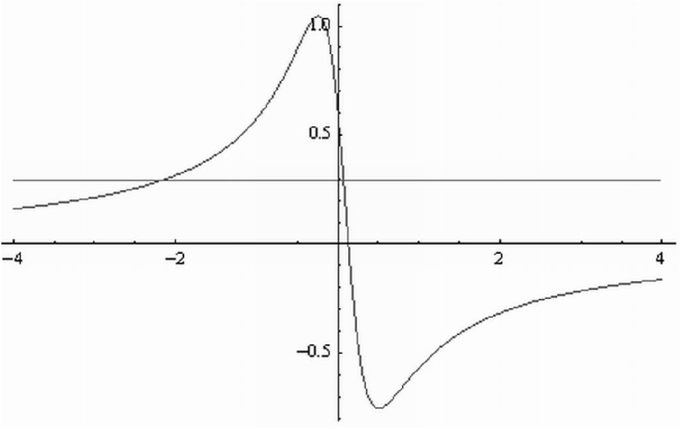
Given the explicit expression for in formula (4), we can plot it (see Fig. 1, where artificial data is used with which is drawn as a horizontal line). There are some general properties in : it is defined throughout the real axis, has two extrema, and the real axis is an asymptote to it.
3 Regression equation with three predictors
Now consider the case of one outcome and three predictors . The point of interest is predictor the other predictors being confounders. We want to get an interpretation of coefficient at the variable of interest in the multiple regression equation
| (5) |
We can introduce the regression equation of on covariates :
and define a new variable by the formula
| (6) |
As in section 1, we could find a simple regression equation for on covariate
| (7) |
Similar to Theorem 2, we have the following statement.
The proof of this theorem is given in Appendix 3.
Going over to a more general case, we can define covariate as follows
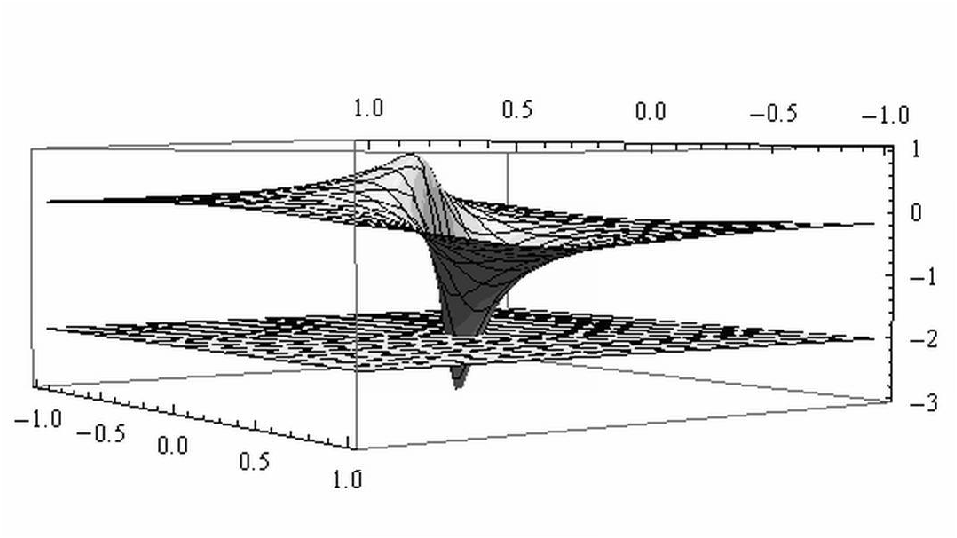
where are some real numbers. Then regression coefficient becomes a function of two real variables . The shape of surface is shown in Figure 2 (using simulated data with ).
4 Applications to real data analysis
4.1 Regression with two predictors
Let us consider the use of Theorem 2 for investigating the dependency of incidence on various air pollution toxicants of City St.-Petersburg (Russia). The primary data were published in Scherbo (2002). In the remainder of this section, we assume incidence to be incidence rate in the adult population (i.e. the number of disease cases per 1000 adult population a year) averaged over a 5-year observation period. In the primary data, the rates of incidence were gathered across 19 boroughs of St.-Petersburg. We consider toxicant concentrations as random variables, i.e. mean toxicant concentration expressed in maximum concentration limit (MCL) terms and averaged over 5-year observation period. Each of these variables takes on 19 values in accordance with the number of boroughs. We denote these covariates by the usual chemical notations: etc. (the data consists of 12 pollutants).
The simple linear regression equations of response (incidence) on concentrations of and are given by
| (8) |
| (9) |
According to equation (8), incidence increases by 579 cases per 1000 population at an increase in concentration by MCL unit a year. Equation (9) may be interpreted in the same way. In short, both and increase incidence.
There is a tight positive correlation between predictors and . Pearson’s correlation coefficient is 0.75, and the regression equation is
This shows that growth in one toxicant is related to growth in another. Hence, one can conjecture that equation (8) does describe an increase in incidence at a simultaneous increase in both pollutants ( and ). A question then arises: could one specify the ‘pure’ influence of each toxicant on incidence, separating the contribution of one toxicant from that of the other?
To extract the contribution of each toxicant to the incidence in the presence of other toxicants, researchers often use a multiple regression equation including all toxicants. Such interpretation is common in some biological and medical applications of regression analysis. We refer to McNamee (2005) as a typical exposition. In the case under consideration, we obtain a multiple regression equation
| (10) |
A lot of authors consider the coefficients of a multiple regression equation obtained by means of the least squares method to be meaningless if there are correlations among predictors (Draper and Smith (1998), Aivazian et al. (1985), Ehrenberg (1975)). These coefficients cannot be used to assess separately the dependence of on and on . Nevertheless, there are other authors who treat each coefficient of a multiple regression equation as the contribution of an individual toxicant to the outcome against the background of other toxicants (e.g. McNamee (2005)). Moreover, this contribution has to be refined as compared to (8)–(9). Their supposition is that predictors as if distribute their influence on the outcome in a multiple regression equation so that each predictor describes its influence with the other being in the background. According to this viewpoint, the addition of another toxicant, , to and change from (8) to (10) should attenuate the effect of because the corresponding coefficient diminished from 579 to 390. The same conclusion holds for and and equations (9) and (10).
These authors do not provide any substantive explanation for the biomedical meaning of variations in the coefficients in (8)–(9) and (10); nor do they explain the refined contribution of each individual toxicant. Variations in regression coefficients could be explained by going over from simple regressions (8) or (9) to multiple regression (10). Indeed, coefficient in equation (10) is equal to coefficient in the simple regression equation
where covariate is defined by
| (11) |
By (11), predictor is obtained from by excluding its part correlated with . Then means an increased incidence rate at a growth in concentration excluding the linear statistical dependence of and .
One can similarly treat coefficient in (10). It is equal to in the simple regression equation
where is a part of toxicant which contains no linear statistical dependence on
We seem to have obtained a consistent picture: by excluding the (linear) dependence of one toxicant on the other we arrive at a ‘pure’ influence of a particular factor on incidence. Since both factors increase the incidence, and the concentration of each factor increases with growth in the other, one can anticipate that the magnitudes of the coefficients in equation (10) should be less than in (8)–(9). This is exactly so in the case under consideration.
It is not as simple as that though. Let us consider the dependence of incidence on the concentrations of and . A simple regression equation of on is given by
The association between and is very similar to that between and . For instance, the correlation coefficient is 0.73 and the regression equation is
| (12) |
The multiple regression equation in the case considered is (Varaksin et al. (2004))
| (13) |
Assuming the coefficients of (13) to be refined ones we should treat the magnitude 1047 as a ‘pure’ influence of against the background of , and as a ‘pure’ influence of against the background of Obviously, such interpretation of regression coefficients is invalid, since the ‘pure’ influence of toxicant becomes negative. The reason for such misinterpretation is the tight correlation between predictors and . One has to take into account this correlation in treating regression coefficients.
The coefficient at in (13) is twice as large as that in (8). By Theorem 2, coefficient is equal to the slope in
| (14) |
where . In biomedical terms, we obtain an inexplicable picture: we have reduced the toxic burden on the population by removing one of the two toxicants, but the incidence grows with even more rapidly. In mathematical terms, we can explain this as follows. It is clear from the definition of that its range is less than the range of In both cases, the incidence is the same, which implies an increase in coefficient . Generally, inequality is impossible if we consider the multiple regression coefficients as refined ones. But if we refer to equality (23), we can see that under and correlation coefficient close to 1, inequality may hold true. The formula (24) also explains the possibility of a negative value for coefficient .
4.2 Regression with three predictors
Let us consider a regression equation of incidence on three predictors and By the least square method, we obtain the equation
Equation (5) becomes
The new variable is defined by (6), and the simple regression equation for on this predictor is given by
We see that as well.
5 Conclusion
Let there be two regression equations for outcome
and
If predictors are uncorrelated, then . Hence, inequality is caused by the presence of correlation between the predictors. What is the epidemiological meaning of changing coefficient to after adding predictor to the simple regression model? Is the influence of the predictors on the outcome redistributed between them? The answer is definitely ‘no’. Usually, the addition of a second covariate is aimed at taking into account the combined effect of predictors on outcome. But what does ‘take into account’ mean? There are no reasonable explanations of this term.
In view of Theorem 2 we can state that the addition of to regression equation brings us to regression equation . The new variable contains no linear statistical dependence on . A similar interpretation holds for the case of three variables as well as for the general one.
Acknowledgement
The research was supported by Basic Science Research for Medicine Program through the Ural Division of RAS Presidium (12--2-1033).
Appendix 1
Proof of the Theorem 2
Let us first prove a technical statement, being of significance in its own right. Let there be a set of predictors and let be an outcome. The values of observations over predictors and the outcome combine into matrices and
The first column contains unities so that we have the same formulae for calculating in the same way as other Let denote the column of coefficients . To find a linear regression equation for response from predictors , we have to minimize the mean square residual of and i.e.
| (15) |
where the T denotes matrix transposition. The problem (15) has a unique solution under the usual least squares method assumptions, e.g. if the matrix is invertible (see e.g. Draper and Smith (1998)[Chapter 5]). Such assumption will be needed throughout Appendix 1.
Let denote a nonsingular square matrix of order
and let be a matrix of order
Let us introduce a vector, , and consider linear transformation of variables by the matrix
| (16) |
Thus, the new variables obtained from variables by means of linear transformation are given by
Finally, we denote by a matrix constructed from in the same way as from , and stands for the column of coefficients .
Proposition 1. Let multiple regression equation of outcome on predictors be
Then coefficients of the multiple regression equation for on predictors
can be found from the matrix equality
It is easy to check that under condition (16) we have
| (17) |
To find a regression equation relative to new variables we need to solve the minimization problem
Given equality (17), we have
Hence we obtain , since the minimization problem (15) has a unique solution. It is obvious from its definition that matrix is invertible and
This brings us to the end of the proof of the Proposition.
Proof To prove Theorem 2, consider the case of two predictors , , and matrix is equal to
Then and . Applying the Proposition to matrix we obtain
| (18) |
It can be easily seen that and are uncorrelated (correlation coefficient is equal to zero). Therefore, coefficients of the multiple regression equation for outcome on predictors
are equal to the corresponding coefficients of the simple regression equations for on predictors and , respectively
| (19) |
Appendix 2
Proof of the Theorem 2
Let us consider linear transformation of variable
| (20) |
Then in the regression equation
| (21) |
coefficient becomes a function of parameter . Its explicit expression is given by
| (22) |
Proof (of Theorem 2) Recall the following regression equations for outcome on predictors (jointly and separately)
and we introduce matrices
where are regression coefficients from the equations
According to the theorem Panov and Varaksin (2010), we have equality . Now, suppose that is an invertible matrix (the opposite case is discussed below in the RemarkProof of the Theorem ). Then
Thus we obtain the following representation of regression coefficients ( denotes the correlation coefficient between )
| (23) |
| (24) |
| (25) |
If we equate the right hand side of (23) to the right hand side of (22), we obtain the roots of the equation (after some simplification)
Applying (25), we get
where .
Next, we expand the second summand in the radicand and factor out the . After that, is substituted by (see (25)). We get
or
Applying (25) again, we obtain the required equalities
That is
or
Remark If correlation matrix is singular, then , i.e. predictors are proportional. In this case, the problem of finding a multiple regression equation on variables cannot be posed, since it leads to an inconsistent system of linear equations.
Appendix 3
Proof of the Theorem 3
The method of proving Theorem 3 as considered in this Appendix contains the main ideas of the proof of the general statement.
Let the linear multiple regression equation for outcome on predictors be
We introduce new variable by
where are some constants. So we perform linear transformation of predictors by the matrix
The inverse matrix is equal to
Hence the coefficients of the regression equation for on and that on are connected by (see Appendix 1)
| (26) |
In particular, for arbitrary coefficients and are equal. From now on we assume .
Let us consider a simple regression equation for on
We have divided the proof of Theorem 3 into a sequence of lemmas.
Lemma 1. The multiple correlation coefficient of variable on predictors is equal to zero.
Proof Let be the multiple correlation coefficient of on variables . By its definition
where is the determinant of the correlation matrix of variables , is the cofactor of the (1,1) entry of the matrix Therefore
Similar to the case of two predictors, one can see that Hence
i.e.
Lemma 2. Let us have multiple regression equations for outcome Y on variables
| (27) |
and that on variables
Also, consider simple regression equations for outcome Y on predictors and respectively
Then
Besides,
| (28) |
where is the regression coefficient from equation (2).
Proof. As it is mentioned above, covariates are uncorrelated as well as . Hence . The last equality (28) is implied by Theorem 2.
Lemma 3. Let there be a multiple regression equation for variable
| (29) |
Then
For the multiple regression equation of on predictors
we have
Proof We obtain it by a tedious calculation. By the least squares method, coefficient can be obtained from a system of linear equations. The numerator of the expression for is the determinant
| (30) |
From corresponding systems of linear equations we obtain
After substituting these into (30) and making necessary simplifications we thus obtain .
The second equality is proved in just the same way.
Proof of Theorem 3 By (26) we have . Lemma Proof of the Theorem shows that . In what follows we need an appropriate generalization of the theorem Panov and Varaksin (2010). It is provided below in Appendix 4. Applying it, we get
| (31) |
This proves Theorem 3, since by lemma Proof of the Theorem .
Appendix 4
A theorem on relationship among regression coefficients
What follows is a statement of the theorem used in Appendix 3.
Theorem (Panov, ) Let there be an outcome Y and a set of predictors . Consider a multiple regression equation for the outcome on the set of predictors
| (32) |
From the set of predictors , we extract a subset and introduce regression equations for each predictor on the subset of predictors extracted
| (33) |
We suppose that for .
Finally, let there be a multiple regression equation for outcome Y on the set of predictors
| (34) |
Then
| (35) |
This theorem has been used in Appendix 3 as follows. The set of all predictors is , the extracted set of predictors is . Then (32) becomes the equation (see 26)
Thus (35) becomes (for )
References
- Aivazian et al. (1985) Aivazian, S. A., Yenyukov, I. S., and Meshalkin, L. D. (1985). Applied statistics. Study of Relationships. Finansy i statistika.
- Draper and Smith (1998) Draper, N. R. and Smith, H. (1998). Applied Regression Analysis. John Wiley & Sons, 3rd edition.
- Ehrenberg (1975) Ehrenberg, A. S. C. (1975). Data Reduction. John Wiley & Sons.
- McNamee (2005) McNamee, R. (2005). Regression modelling and other methods to control confounding. Occup. Environ. Med., 62:500–506.
- Nalimov (1975) Nalimov, V. V. (1975). Theorie des Experiments. VEB Deutscher Landwirtschaftsverlag, Berlin.
- (6) Panov, V. G. On relationship among coefficients of the linear regression models of different dimentions. In Press.
- Panov and Varaksin (2010) Panov, V. G. and Varaksin, A. N. (2010). Relation between the coefficients of simple and multiple regression models. Siberian Mathematical Journal, 51(1):162–167.
- Scherbo (2002) Scherbo, A. P., editor (2002). Environment and Health: Approaches to assessment of health risk. St-Petersburg MAPO, Saint-Petersburg.
- Varaksin et al. (2004) Varaksin, A. N., Maslakova, T. A., Chukanov, V. N., and Antonov, K. L. (2004). The regression model for dependence of population disease incidence from rate of atmospheric air pollution. Ecological Systems and Devices, 4:52–55.