跳到论文正文
W Papers独立论文阅读器 arXiv:1205.2390 论文正文 计算阅读时间 · 0%
引用这篇论文根据当前论文元数据生成,正式投稿前建议核对。


License: arXiv.org perpetual non-exclusive license
arXiv:1205.2390v1 [quant-ph] 09 May 2012

Quantum Ternary Circuit Synthesis Using Projection Operations

Sudhindu Bikash Mandal Email: sudhindu.mandal@gmail.com Affiliation: A. K. Choudhury School of Information Technology, University of Calcutta, India    Amlan Chakrabarti1   
Susmita Sur-Kolay
Affiliation: Advanced Computing & Microelectronics Unit, Indian Statistical Institute, India
Abstract

Basic logic gates and their operations in ternary quantum domain are involved in the synthesis of ternary quantum circuits. Only a few works define ternary algebra for ternary quantum logic realization. In this paper, a ternary logic function is expressed in terms of projection operations including a new one. A method to realize new multi-qutrit ternary gates in terms of generalized ternary gates and projection operations is also presented. We also introduced ten simplification rules for reducing ancilla qutrits and gate levels. Our method yields lower gate cost and fewer gate levels and ancilla qutrits than that obtained by earlier methods for the ternary benchmark circuits. The nn qutrit ternary sum function is synthesized without any ancilla qutrit by our proposed methodology.

keywords
Gate level logic synthesis, Ternary quantum circuits, Projection operations

1 Introduction

Multi-valued quantum computing is gaining importance in the field of quantum information theory and quantum cryptography as it can represent an n-dimensional quantum system, defined by the basis states |0>|0>, |1>|1>, …, |n−1>|n-1>. The unit of information is called a qudit. A qudit exists as a linear superposition of states, and is characterized by a wave function ψ\psi [1, 2].

Multi-valued quantum algebra comprises the rules for a set of basic logic operations that can be performed on qudits. While in [3] the structure of a multi-valued logic gate is proposed which can be experimentally feasible with a linear ion trap scheme for quantum computing, this approach produces large dimensional circuits. A universal architecture for multi-valued reversible logic is given in [4], but quantum realization of the circuits thus obtained is not apparent. The universality of nn-qudit gates is presented in [5], but no algorithms for synthesis were given. Al-Rabedi proposed in [6] the minimization technique for multi-valued quantum galois field sum of product.

In this paper we concentrate on the quantum ternary functions. A ternary quantum system exists in linear superposition of three basis states, labeled |0>|0>, |1>|1> and |2>|2>. All the operations on a qutrit are developed in a 3-dimensional Hilbert space under the field GF(3) [7]. A two qutrit vector can be represented as |ψ>|\psi> = ∑i=08|Ci|2\sum^{8}_{i=0}|C_{i}|^{2} = 1. In general, a nn qutrit state can be represented as a superposition of 3n3^{n} basis states. A quantum register of size nn qutrits can hold 3n3^{n} values simultaneously, whereas the nn-qubit register in binary quantum domain can hold 2n2^{n} values. For the same size of memory, a Quantum Fourier Transform (QFT) with ternary qutrits improves the approximation and increases the state space by a factor of (3/2)n(3/2)^{n} [8]. This is very useful in cryptography.

The realization of ternary operations requires a set of universal gates with which a quantum circuit for a given ternary quantum function can be built. One set of universal gates [9] comprise the Ternary Swap, the Ternary NOT and the Ternary Toffoli gate. With these universal gates, any arbitrary quantum circuit can be realized without ancilla bits, but this approach is not optimal in terms of quantum cost [9]. Further, the synthesis method in [10] uses quantum multiplexers and the method of iterative deepening depth first search is employed to minimize the gate cost. Another synthesis technique was proposed in [11] for garbage free GF(3) based reversible or quantum logic circuit from its truth values, using only Muthukrishnan-Stroud (M-S) [3] and shift gates [12]. But this technique did not provide any simplification rule to reduce the gate count. In paper [13] the ternary quantum logic was expressed in terms of Ternary Galois Field Sum of Product, and 16 Ternary Galois Field expansions were also proposed. But this paper did not provide any gate level implementation of ternary benchmark circuit.

The paper here is the extended version of [14], where our motivation is to synthesis a given quantum ternary benchmark [13] function specified as ternary minterms, using projection operations. Further we realize the gate level implementation of these benchmark [13] circuits using Generalized Ternary Gates [8] and newly defined permutative ternary quantum C2NOT gates. A few simplification rules are enumerated for reducing the number of ancilla qutrits and the levels of gates in the resulting quantum circuit.

The preliminary concepts of ternary algebra with a new projection operation appear in Section 2. In Section 3, the characteristics of basic ternary logic gates and the Generalized Ternary Gate (GTG) [12] along with the introduction of a few new gates are discussed. The proposed synthesis methodology along with a set of simplification rules is presented in Section 4. Synthesis of quantum ternary benchmark circuits by this method, and the respective quantum gate cost with ancilla qutrit count are given in Section 5. Concluding remarks appear in Section 6.

2 Ternary Algebra

We first define the basic operations over the set {0, 1, 2}.

2.1 Ternary AND, OR, NOT

The operations of AND, OR, and NOT [15] for ternary variables are:
A​N​D​(a,b)={aif a≤b;botherwise.AND(a,b)=\left\{\begin{array}[]{ll}\mbox{$a$}&\mbox{if $a\leq b$};\\ \mbox{$b$}&\mbox{otherwise}.\\ \end{array}\right. O​R​(a,b)={aif a≥b;botherwise.OR(a,b)=\left\{\begin{array}[]{ll}\mbox{$a$}&\mbox{if $a\geq b$};\\ \mbox{$b$}&\mbox{otherwise}.\\ \end{array}\right.
N​O​T​(a)=a+1NOT(a)=a+1.
Here ′+′{}^{\prime}+^{\prime} denotes the modulo 3 addition. It is easy to see that the ternary A​N​DAND operation is distributive over the O​ROR operation and vice-versa [15].

2.2 Ternary Projection Operations LiL_{i} and JiJ_{i}

Our main goal is to define a given ternary function in terms of the minterms corresponding to its 11 or 22 values. The 3n3^{n} minterms for a function ff with nn ternary variables are denoted by m0m_{0} to m3n−1m_{3^{n}-1}. In the sum of products form of minterms, the minterm m0m_{0} = ∏inN​O​T​(xi)\prod^{n}_{i}NOT(x_{i}) where xx = {00, 11, 22} and ∏\prod denotes the ternary A​N​DAND; its value is 1, 2, or 0 depending on whether for all i xix_{i} = 0, 1 or 2 respectively.

As the outcomes of a ternary function may be 00, 11 or 22, we cannot express a ternary function ff which results in either 11 or 22 for a given set of inputs, by using the above minterms mim_{i}. So, we present six projection operations, grouped into two types LiL_{i} and JiJ_{i}, where ii = {00, 11, 22}. While the JiJ_{i} type operation was defined earlier [15] as

Ji​(a)={2if a=i;0otherwise.J_{i}(a)=\left\{\begin{array}[]{ll}\mbox{$2$}&\mbox{if $a=i$};\\ \mbox{$0$}&\mbox{otherwise}.\\ \end{array}\right.

the LiL_{i} types are newly defined here as

Li​(a)={1if a=i;0otherwise.L_{i}(a)=\left\{\begin{array}[]{ll}\mbox{$1$}&\mbox{if $a=i$};\\ \mbox{$0$}&\mbox{otherwise}.\\ \end{array}\right.

Their truth tables appear in Table 1. From Table 1, we can verify that the output of any LiL_{i} operation is either 00 or 11, and that of JiJ_{i} operation is either 00 or 22. Two other derived operations Li′L^{\prime}_{i}, Ji′J^{\prime}_{i} as shown in the Table 2. Next, we express a ternary function as a sum of products minterm form by using the LiL_{i} and JiJ_{i} operations. The LiL_{i} and JiJ_{i} operations are commutative, associative and distributive over ternary AND and OR logic. We can verify these laws given below, from Table 1. Here ii, jj, kk = {0, 1, 2}
1. Commutativity
(i) Li​(a)+Lj​(b)L_{i}(a)+L_{j}(b) = Lj​(b)+Li​(a)L_{j}(b)+L_{i}(a) Ji​(a)+Jj​(b)J_{i}(a)+J_{j}(b) = Jj​(b)+Ji​(a)J_{j}(b)+J_{i}(a) (ii) Li​(a).Lj​(b)L_{i}(a).L_{j}(b) = Lj​(b).Li​(a)L_{j}(b).L_{i}(a) Ji​(a).Jj​(b)J_{i}(a).J_{j}(b) = Jj​(b).Ji​(a)J_{j}(b).J_{i}(a)
2. Associativity
(i) [Li​(a)+Lj​(b)L_{i}(a)+L_{j}(b)]+ Lk​(c)L_{k}(c) = Li​(a)L_{i}(a)+ [Lj​(b)+Lk​(c)L_{j}(b)+L_{k}(c)] [Ji​(a)+Jj​(b)J_{i}(a)+J_{j}(b)]+ Jk​(c)J_{k}(c) = Ji​(a)J_{i}(a)+ [Jj​(b)+Jk​(c)J_{j}(b)+J_{k}(c)] (ii) [Li​(a).Lj​(b)L_{i}(a).L_{j}(b)].Lk​(c)L_{k}(c) = Li​(a)L_{i}(a). [Lj​(b).Lk​(c)L_{j}(b).L_{k}(c)] [Ji​(a).Jj​(b)J_{i}(a).J_{j}(b)].Jk​(c)J_{k}(c) = Ji​(a)J_{i}(a). [Jj​(b).Jk​(c)J_{j}(b).J_{k}(c)]
3. Distributivity
(i)  Li​(a)L_{i}(a).[Li​(b)+Lk​(c)L_{i}(b)+L_{k}(c)]=Li​(a).Lj​(b)+Li​(a).Lk​(c)L_{i}(a).L_{j}(b)+L_{i}(a).L_{k}(c)
  Ji​(a)J_{i}(a).[Ji​(b)+Jk​(c)J_{i}(b)+J_{k}(c)]=Ji​(a).Jj​(b)+Ji​(a).Jk​(c)J_{i}(a).J_{j}(b)+J_{i}(a).J_{k}(c)
(ii) Li​(a)L_{i}(a)+ [Lj​(b)+Lk​(c)L_{j}(b)+L_{k}(c)] = [Li​(a)+Lj​(b)L_{i}(a)+L_{j}(b)].[Li​(a)+Lk​(c)L_{i}(a)+L_{k}(c)]
   Ji​(a)J_{i}(a)+ [Jj​(b)+Jk​(c)J_{j}(b)+J_{k}(c)] = [Ji​(a)+Jj​(b)J_{i}(a)+J_{j}(b)].[Ji​(a)+Jk​(c)J_{i}(a)+J_{k}(c)]

aa L0​(a)L_{0}(a) L1​(a)L_{1}(a) L2​(a)L_{2}(a) J0​(a)J_{0}(a) J1​(a)J_{1}(a) J2​(a)J_{2}(a)
0 1 0 0 2 0 0
1 0 1 0 0 2 0
2 0 0 1 0 0 2
Table 1: Truth tables of ternary projection operations LiL_{i} and JiJ_{i}
aa L0′​(a)L^{\prime}_{0}(a) L1′​(a)L^{\prime}_{1}(a) L2′​(a)L^{\prime}_{2}(a) J0′​(a)J^{\prime}_{0}(a) J1′​(a)J^{\prime}_{1}(a) J2′​(a)J^{\prime}_{2}(a)
0 0 1 1 0 2 2
1 1 0 1 2 0 2
2 1 1 0 2 2 0
Table 2: Truth tables of ternary operations Li′L^{\prime}_{i} and Ji′J^{\prime}_{i}

3 Ternary Logic Gates

3.1 Ternary Feynman, Ternary Toffoli, MAX and MIN gates

The two qutrit ternary Feynman gate [16], shown in Figure 1, is defined as
Feynman(AA, BB) = AA + BB
where ’+’ operator is addition over GF(3).

The ternary 3-qutrit Toffoli gate [16] in the universal ternary quantum get set, is shown in Figure 2 and is defined as
T​o​f​f​o​l​i​(CLOSEToffoli(A,B,C)={Z operation on Cif A = B = 2;Cotherwise;)=\left\{\begin{array}[]{ll}\mbox{$Z$ operation on $C$}&\mbox{\emph{if A = B = 2}};\\ \mbox{$C$}&\mbox{otherwise};\\ \end{array}\right.
where AA, BB are controlling input and ZZ ={+1+1, +2+2, 0101, 0202, 1212}.

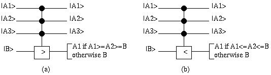
In our synthesis method, ternary SWAP and NOT gates are not used explicitly. Instead, we use the ternary MAX and MIN gates [10] respectively to replace the OR and the AND in ternary quantum logic. These two gates are defined as
MAX(A1,A2,..,An,MAX(A_{1},A_{2},..,A_{n},B)={Aiif Ai ≥ Aj, i≠j and Ai ≥ B;Bif ∀i,B≥Ai;)=\left\{\begin{array}[]{ll}\mbox{$A_{i}$}&\mbox{if $A_{i}$ $\geq$ $A_{j}$, $i\neq j$ and $A_{i}$ $\geq$ $B$};\\ \mbox{$B$}&\mbox{if $\forall i,B\geq A_{i}$};\\ \end{array}\right.

M​I​N​(A1,A2,…​AnCLOSE,MIN(A_{1},A_{2},...A_{n},B)={Aiif Ai ≤ Aj, i≠j and Ai≤B;Bif ∀i,B≤Ai;)=\left\{\begin{array}[]{ll}\mbox{$A_{i}$}&\mbox{if $A_{i}$ $\leq$ $A_{j}$, $i\neq j$ and $A_{i}\leq B$};\\ \mbox{$B$}&\mbox{if $\forall i,B\leq A_{i}$};\\ \end{array}\right.
where ii = {1,2,…​n}\{1,2,\ldots n\} (Figure 3).

The ternary Toffoli gate can be realized without any ancilla qutrits [16, 17] by using Muthukrishnan-Stroud gates (M-S gate) and . An M-S gate is defined as
M-S(A,B)={B shift by Zif A = 2;Botherwise;(A,B)=\left\{\begin{array}[]{ll}\mbox{B shift by Z}&\mbox{if A = 2};\\ \mbox{B}&\mbox{otherwise};\\ \end{array}\right.
where ZZ = {+1+1, +2+2, 0101, 0202, 1212} [15] (Figure 4(a)).

Refer to caption
Figure 1: 2 qutrit ternary Feynman Gate
Refer to caption
Figure 2: 3 qutrit ternary Toffoli Gate
Refer to caption
Figure 3: Ternary Multi-qutrit (a) M​A​XMAX gate, and (b) M​I​NMIN gate
Refer to caption
Figure 4: (a) A Muthukrishnan-Stroud (M-S) gate, and (b) a Generalized Ternary Gate (GTG)
Table 3: Ternary Shift operations used in a GTG
Shift gate Its operation
Buffer xx = xx
Single Shift xx = x+1x+1
Dual Shift xx = x+2x+2
Self Shift xx = 2​x2x
Self Single Shift xx = 2​x+12x+1
Self Dual Shift xx = 2​x+22x+2

3.2 Generalized Ternary Gate

In order to realize a Generalized ternary gate (GTG) defined next, the Shift gates [12] given in Table 3 are required. Here addition and multiplication over G​F​(3)GF(3) are denoted by ’++’ and ’.’ respectively.

A Generalized Ternary Gate (GTG) is a 2-qutrit gate, as shown in Figure 4(b). The controlling input of a GTG can be used to select the 1-qutrit shift operation on the target input. The GTG is defined as
G​T​G​(A,B)={B shift Xif A=0;B shift Yif A=1;B shift Zif A=2GTG(A,B)=\left\{\begin{array}[]{lll}\mbox{B shift X}&\mbox{if A=0};\\ \mbox{B shift Y}&\mbox{if A=1};\\ \mbox{B shift Z}&\mbox{if A=2}\end{array}\right.

where XX, YY, and ZZ are any three distinct shift operations in Table 3.

3.2.1 Implementation of LiL_{i} and JiJ_{i} operations using GTG

We can implement the LiL_{i} and JiJ_{i} projection operations defined in Section 2.2, by using GTG as shown in Figures 5 (a) and (b) respectively. For the LiL_{i} type operation, we set b=1b=1.
Li​(a)=G​T​G​(a,b)={bif a=i;b+2if a=i+1;2b+1if a=i+2L_{i}(a)=GTG(a,b)=\left\{\begin{array}[]{lll}\mbox{b}&\mbox{if a=i};\\ \mbox{b+2}&\mbox{if a=i+1};\\ \mbox{2b+1}&\mbox{if a=i+2}\end{array}\right.

For the JiJ_{i} type operation, we set b=2b=2.
Ji​(a)=G​T​G​(a,b)={bif a=i;b+1if a=i+1;2b+2if a=i+2J_{i}(a)=GTG(a,b)=\left\{\begin{array}[]{lll}\mbox{b}&\mbox{if a=i};\\ \mbox{b+1}&\mbox{if a=i+1};\\ \mbox{2b+2}&\mbox{if a=i+2}\end{array}\right.

Refer to caption
Figure 5: Realization of ternary (a) LiL_{i} operation and (b) JiJ_{i} operation with GTGs
Refer to caption
Figure 6: Realization of ternary JiJ_{i} operation wth GTG

3.3 A new Ternary C2​N​O​TC^{2}NOT gate

Several multi-qutrit control operations are possible in ternary logic. We present a new definition of a 3-qutrit C2​N​O​TC^{2}NOT (Figure 6(a)), which is required to realize the simplification rules for ternary minterms given in the Section 4.2 below, as
C2​N​O​T​(A,B,C)={NOT(C)if A≠B and A,B≠0 ;Cotherwise;C^{2}NOT(A,B,C)=\left\{\begin{array}[]{ll}\mbox{NOT(C)}&\mbox{if $A\neq B$ and $A$,$B\neq 0$ };\\ \mbox{C}&\mbox{otherwise};\\ \end{array}\right.
where AA and BB are the control inputs, and CC the target input. The realization of this C2​N​O​TC^{2}NOT gate with M-S gates is shown in Figure 6(b).

Refer to caption
Figure 7: (a) The proposed ternary C2​N​O​TC^{2}NOT gate, and (b) its realization with M-S gates

3.4 A Multi-qutrit GTG

We also define a Multi-qutrit GTG (Figure 7) as
GTG(A1,A2,..,AnA_{1},A_{2},..,A_{n}, B)={B shift Xif A1,A2,..,An=0;B shift Yif A1,A2,..,An=1;B shift Zif A1,A2,..,An=2;Botherwise;\left\{\begin{array}[]{llll}\mbox{B shift X}&\mbox{if $A_{1},A_{2},..,A_{n}$=0};\\ \mbox{B shift Y}&\mbox{if $A_{1},A_{2},..,A_{n}$=1};\\ \mbox{B shift Z}&\mbox{if $A_{1},A_{2},..,A_{n}$=2};\\ \mbox{B}&\mbox{otherwise};\end{array}\right.

Refer to caption
Figure 8: The proposed Multi-qutrit GTG

4 Proposed Synthesis Methodology

4.1 Overview

Consider an mm-variable ternary quantum logic function f⁡(a1,a2,…,am)f(a_{1},a_{2},\ldots,a_{m}) = ∑i=0n\sum^{n}_{i=0}(minterms for one )i + ∑j=0p\sum^{p}_{j=0}(minterms for two)j
where ∑\sum implies logical ternary OR, n and p are respectively the number of input vectors for which ff is 11, and 22. Thus, for (3m−n−p)(3^{m}-n-p) input vectors, ff is 0 . We express the minterm for one and two by using the LiL_{i} and JiJ_{i} operations respectively. From Table II, we can say
∏i=1mL0​(ai)\prod^{m}_{i=1}L_{0}(a_{i}) = {1if ∀i ai = 0;0if ∃ i ai = 1 or 2;\left\{\begin{array}[]{ll}\mbox{1}&\mbox{if $\forall i$ $a_{i}$ = 0};\\ \mbox{0}&\mbox{if $\exists$ i $a_{i}$ = 1 or 2};\end{array}\right.
∏i=1mL1​(ai)\prod^{m}_{i=1}L_{1}(a_{i}) = {1if ∀i ai = 1;0if ∃ i ai = 0 or 2;\left\{\begin{array}[]{ll}\mbox{1}&\mbox{if $\forall i$ $a_{i}$ = 1};\\ \mbox{0}&\mbox{if $\exists$ i $a_{i}$ = 0 or 2};\end{array}\right.
∏i=1mL2​(ai)\prod^{m}_{i=1}L_{2}(a_{i}) ={1if ∀i ai = 2;0if ∃ i ai = 0 or 1;\left\{\begin{array}[]{ll}\mbox{1}&\mbox{if $\forall i$ $a_{i}$ = 2};\\ \mbox{0}&\mbox{if $\exists$ i $a_{i}$ = 0 or 1};\end{array}\right.
∏i,p,k=1mL0​(ai).L1​(ap).L2​(ak)\prod^{m}_{i,p,k=1}L_{0}(a_{i}).L_{1}(a_{p}).L_{2}(a_{k}) ={1if ∀i,p,k ai = 0, ap = 1, ak = 2;0if ∃ i, p, k ai = 1 or 2, ap = 0 or 2, ak = 0 or 1;\left\{\begin{array}[]{ll}\mbox{1}&\mbox{if $\forall i,p,k$ $a_{i}$ = 0, $a_{p}$ = 1, $a_{k}$ = 2};\\ \mbox{0}&\mbox{if $\exists$ i, p, k $a_{i}$ = 1 or 2, $a_{p}$ = 0 or 2, $a_{k}$ = 0 or 1};\end{array}\right.
where i+p+k=mi+p+k=m.

Hence, the minterms for which f=1f=1 are
1. ∏i=1mL0​(ai=0)\prod^{m}_{i=1}L_{0}(a_{i}=0),
2. ∏i=1mL1​(ai=1)\prod^{m}_{i=1}L_{1}(a_{i}=1),
3. ∏i=1mL2​(ai=2)\prod^{m}_{i=1}L_{2}(a_{i}=2), and
4. ∏i,p,k=1mL0​(ai=0).L1​(ap=1).L2​(ak=2)\prod^{m}_{i,p,k=1}L_{0}(a_{i}=0).L_{1}(a_{p}=1).L_{2}(a_{k}=2).

Similarly from Table I, the minterms for which f=2f=2 are
1. ∏i=1mJ0​(ai=0)\prod^{m}_{i=1}J_{0}(a_{i}=0),
2. ∏i=1mJ1​(ai=1)\prod^{m}_{i=1}J_{1}(a_{i}=1),
3. ∏i=1mJ2​(ai=2)\prod^{m}_{i=1}J_{2}(a_{i}=2), and
4. ∏i,p,k=1mJ0​(ai=0).J1​(ap=1).J2​(ak=2)\prod^{m}_{i,p,k=1}J_{0}(a_{i}=0).J_{1}(a_{p}=1).J_{2}(a_{k}=2).

4.2 Simplification Rules

Next, we define seven simplification rules for our proposed method, the first four are derived from Table 1, and the next three from Table 2.
1. Li​(a)​.0=0L_{i}(a).0=0, and Ji​(a)​.0=0J_{i}(a).0=0
2. Li​(a)​.1=Li​(a)L_{i}(a).1=L_{i}(a), and Ji​(a)​.2=Ji​(a)J_{i}(a).2=J_{i}(a)
3. Li​(a)+0=Li​(a)L_{i}(a)+0=L_{i}(a), and Ji​(a)+0=Ji​(a)J_{i}(a)+0=J_{i}(a)
4. Li​(a)+1=1L_{i}(a)+1=1, and Ji​(a)+2=2J_{i}(a)+2=2
5. Li​(a).Li′​(a)=0L_{i}(a).L^{\prime}_{i}(a)=0, and Ji​(a).Ji′​(a)=0J_{i}(a).J^{\prime}_{i}(a)=0
6. Li​(a)+Li′​(a)=1L_{i}(a)+L^{\prime}_{i}(a)=1, and Ji​(a)+Ji′​(a)=2J_{i}(a)+J^{\prime}_{i}(a)=2
7. Li′​(a)=Li+1​(a)+Li+2​(a)L^{\prime}_{i}(a)=L_{i+1}(a)+L_{i+2}(a), and Ji′​(a)=Ji+1​(a)+Ji+2​(a)J^{\prime}_{i}(a)=J_{i+1}(a)+J_{i+2}(a).

4.2.1 Simplification Rules for reducing ancilla qutrits

For gate level realization of the projection operations LiL_{i} and JiJ_{i}, we need an ancilla qutrit for each. Further, to synthesize an mm-variable ternary function with nn minterms specified according to our proposed methodology, we have maximum of n∗mn*m ancilla qutrits. However, we can reduce the number of ancilla qutrits by the following three simplification rules based on the new ternary C2​N​O​TC^{2}NOT gate and Table 2:
8. L1​(a)​L2​(b)+L2​(a)​L1​(b)=C2​N​O​T​(a,b,0)L_{1}(a)L_{2}(b)+L_{2}(a)L_{1}(b)=C^{2}NOT(a,b,0) and J1​(a)​J2​(b)+J2​(a)​J1​(b)=C2​N​O​T​(a,b,1)J_{1}(a)J_{2}(b)+J_{2}(a)J_{1}(b)=C^{2}NOT(a,b,1)
9. Li​(a).Li​(a)=Li​(a)L_{i}(a).L_{i}(a)=L_{i}(a) and Ji​(a).Ji​(a)=Ji​(a)J_{i}(a).J_{i}(a)=J_{i}(a)
10. Li(a1)Li(a2)..Li(an)=Li(a1,a2,..,an)L_{i}(a_{1})L_{i}(a_{2})..L_{i}(a_{n})=L_{i}(a_{1},a_{2},..,a_{n}) and Ji(a1)Ji(a2)..Ji(an)=Ji(a1,a2,..,an)J_{i}(a_{1})J_{i}(a_{2})..J_{i}(a_{n})=J_{i}(a_{1},a_{2},..,a_{n}), i={0,1,2}i=\{0,1,2\}.

The multiqutrit LiL_{i} and JiJ_{i} operations in Rule 10 can be realized using Multiqutrit GTG as follows:
For Li(a1,a2,..,an)L_{i}(a_{1},a_{2},..,a_{n}), GTG(a1,a2,..,an,B)={B +1if a1,a2,..,an=i;Bif a1,a2,..,an=i+1;2Bif a1,a2,..,an=i+2;Botherwise;GTG(a_{1},a_{2},..,a_{n},B)=\left\{\begin{array}[]{llll}\mbox{B +1}&\mbox{if $a_{1},a_{2},..,a_{n}$=i};\\ \mbox{B}&\mbox{if $a_{1},a_{2},..,a_{n}$=i+1};\\ \mbox{2B}&\mbox{if $a_{1},a_{2},..,a_{n}$=i+2};\\ \mbox{B}&\mbox{otherwise};\end{array}\right.

For Ji(a1,a2,..,an)J_{i}(a_{1},a_{2},..,a_{n}), GTG(a1,a2,..,an,B)={B +2if a1,a2,..,an=i;Bif a1,a2,..,an=i+1;2Bif a1,a2,..,an=i+2;Botherwise;GTG(a_{1},a_{2},..,a_{n},B)=\left\{\begin{array}[]{llll}\mbox{B +2}&\mbox{if $a_{1},a_{2},..,a_{n}$=i};\\ \mbox{B}&\mbox{if $a_{1},a_{2},..,a_{n}$=i+1};\\ \mbox{2B}&\mbox{if $a_{1},a_{2},..,a_{n}$=i+2};\\ \mbox{B}&\mbox{otherwise};\end{array}\right.

4.3 An Example

For illustrating our method, consider an arbitrary ternary function g⁡(a,b)g(a,b) with its truth table given in Table 4.

Table 4: Truth table for an example ternary 2-qutrit function g⁡(a,b)g(a,b)
a,ba,b 0000 0101 0202 1010 1111 1212 2020 2121 2222
g⁡(a,b)g(a,b) 0 1 2 1 1 1 2 1 2

The disjunction of minterms for which g=1g=1 is
L0​(a)​L1​(b)+L1​(a)​L0​(b)+L1​(a)​L1​(b)+L1​(a)​L2​(b)+L2​(a)​L1​(b)L_{0}(a)L_{1}(b)+L_{1}(a)L_{0}(b)+L_{1}(a)L_{1}(b)+L_{1}(a)L_{2}(b)+L_{2}(a)L_{1}(b)

and that for which g=2g=2 is
J0​(a)​J2​(b)+J2​(a)​J0​(b)+J2​(a)​J2​(b)J_{0}(a)J_{2}(b)+J_{2}(a)J_{0}(b)+J_{2}(a)J_{2}(b).

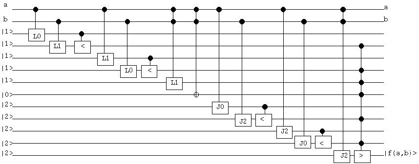
Hence, g⁡(a,b)=L0​(a)​L1​(b)+L1​(a)​L0​(b)+L1​(a)​L1​(b)+L1​(a)​L2​(b)+L2​(a)​L1​(b)+J0​(a)​J2​(b)+J2​(a)​J0​(b)+J2​(a)​J2​(b)g(a,b)=L_{0}(a)L_{1}(b)+L_{1}(a)L_{0}(b)+L_{1}(a)L_{1}(b)+L_{1}(a)L_{2}(b)+L_{2}(a)L_{1}(b)+J_{0}(a)J_{2}(b)+J_{2}(a)J_{0}(b)+J_{2}(a)J_{2}(b).
By simplification rules 1 and 10, we get
g⁡(a,b)=L0​(a)​L1​(b)+L1​(a)​L0​(b)+L1​(a,b)+C2​N​O​T​(a,b,0)+J0​(a)​J2​(b)+J2​(a)​J0​(b)+J2​(a,b).g(a,b)=L_{0}(a)L_{1}(b)+L_{1}(a)L_{0}(b)+L_{1}(a,b)+C^{2}NOT(a,b,0)+J_{0}(a)J_{2}(b)+J_{2}(a)J_{0}(b)+J_{2}(a,b).
The gate level implementation of the function g⁡(a,b)g(a,b) is shown in Figure 8.

Refer to caption
Figure 9: Ternary quantum gate circuit obtained for g⁡(a,b)g(a,b) in Table 4

5 Synthesis of Ternary Benchmark functions

We experimented with the ternary benchmark functions provided in [13]. Their truth tables appear in Table 5. The definition and the synthesis of the ternary benchmark functions using ternary minterm are given in the following subsections.

5.1 2-qutrit multiplication functions m​u​l​2mul2 and m​u​l​2​cmul2c

The functions are defined as
m​u​l​2​(a,b)=a​b​m​o​d​3mul2(a,b)=abmod3, multipication output;
m​u​l​2​c​(a,b)=i​n​t​[a​b/3]mul2c(a,b)=int[ab/3], carry of the multiplier.
The truth table of m​u​l​2​(a,b)mul2(a,b) and m​u​l​2​c​(a,b)mul2c(a,b) appear in columns 33 and 44 respectively of Table 5.
Expressing in terms of projrctin operators, we get
m​u​l​2​(a,b)=L1​(a)​L1​(b)+L2​(a)​L2​(b)+J1​(a)​J2​(b)+J2​(a)​J1​(b)mul2(a,b)=L_{1}(a)L_{1}(b)+L_{2}(a)L_{2}(b)+J_{1}(a)J_{2}(b)+J_{2}(a)J_{1}(b).
      = L1​(a,b)+L2​(a,b)+C2​N​O​T​(a,b,1)L_{1}(a,b)+L_{2}(a,b)+C^{2}NOT(a,b,1) (by Rules 8 and 10)
Similarly, m​u​l​2​c​(a,b)=L2​(a)​L2​(b)=L2​(a,b)mul2c(a,b)=L_{2}(a)L_{2}(b)=L_{2}(a,b) (by Rule 10).

5.2 2-qutrit half-adder t​h​a​d​dthadd

The 2-qutrit half-adder t​h​a​d​dthadd [14] comprises the ternary half adder sum (s​u​m​hsumh) and carry (c​a​r​r​y​hcarryh) functions, whose truth tables are given in columns 5 and 6 respectively of Table 5.
We re-write s​u​m​hsumh according to our proposed methodology as
s​u​m​hsumh = L0​(a)​L1​(b)+L1​(a)​L0​(b)+L2​(a)​L2​(b)+J0​(a)​J2​(b)+J1​(a)​J1​(b)+J2​(a)​J0​(b)L_{0}(a)L_{1}(b)+L_{1}(a)L_{0}(b)+L_{2}(a)L_{2}(b)+J_{0}(a)J_{2}(b)+J_{1}(a)J_{1}(b)+J_{2}(a)J_{0}(b).
Further simplification of s​u​m​hsumh by using the ternary Feynman gate of Section 3.1 gives s​u​m​h=a+bsumh=a+b.
Next, the carry function c​a​r​r​y​hcarryh is written as
c​a​r​r​y​h=L1​(a)​L2​(b)+L2​(a)​L1​(b)+L2​(a)​L2​(b)=C2​N​O​T​(a,b,0)+L2​(a,b)carryh=L_{1}(a)L_{2}(b)+L_{2}(a)L_{1}(b)+L_{2}(a)L_{2}(b)=C^{2}NOT(a,b,0)+L_{2}(a,b) (by Rules 8 and 10).       

Table 5: Truth table of four 22-qutrit benchmark functions[13]
aa bb m​u​l​2mul2 m​u​l​2​cmul2c s​u​m​hsumh c​a​r​r​y​hcarryh s​q​s​u​m​2sqsum2 a​v​g​2avg2
0 0 0 0 0 0 0 0
0 1 0 0 1 0 1 0
0 2 0 0 2 0 1 1
1 0 0 0 1 0 1 0
1 1 1 0 2 0 2 1
1 2 2 0 0 1 2 1
2 0 0 0 2 0 1 1
2 1 2 0 0 1 2 1
2 2 1 1 1 1 2 2

5.3 GF(3) sum of two squares s​q​s​u​m​2sqsum2

The definition of this ternary function is s​q​s​u​m​2​(a,b)=(a2+b2)​m​o​d​3sqsum2(a,b)=(a^{2}+b^{2})mod3 and its truth table is shown in column 7 of Table 5.
s​q​s​u​m​2​(a,b)=L0​(a)​L1​(b)+L0​(a)​L2​(b)+L1​(a)​L0​(b)+L2​(a)​L0​(b)+J1​(a)​J1​(b)+J1​(a)​J2​(b)+J2​(a)​J1​(b)+J2​(a)​J2​(b)sqsum2(a,b)=L_{0}(a)L_{1}(b)+L_{0}(a)L_{2}(b)+L_{1}(a)L_{0}(b)+L_{2}(a)L_{0}(b)+\hskip 65.44133ptJ_{1}(a)J_{1}(b)+J_{1}(a)J_{2}(b)+J_{2}(a)J_{1}(b)+J_{2}(a)J_{2}(b)
       = L0​(a)​L0′​(b)L_{0}(a)L_{0}^{\prime}(b)+L0′​(a)​L0​(b)L_{0}^{\prime}(a)L_{0}(b)+J1​(a,b)+C2​N​O​T​(a,b,2)+J2​(a,b)J_{1}(a,b)+C^{2}NOT(a,b,2)+J_{2}(a,b)
       (by Rules 8, 7 and 10).

5.4 Average function a​v​g​2avg2

The function a​v​g​2avg2 is the integer part of the average of two ternary input variables in m​o​d​u​l​o​3modulo3 and defined as a​v​g​2​(a,b)=i​n​t​[a​b/2]avg2(a,b)=int[ab/2]. Its truth table is in column 8 of Table 5.
a​v​g​2=L0​(a)​L2​(b)+L1​(a)​L1​(b)+L1​(a)​L2​(b)+L2​(b)​L0​(b)+L2​(a)​L1​(b)+J2​(a)​J2​(b)avg2=L_{0}(a)L_{2}(b)+L_{1}(a)L_{1}(b)+L_{1}(a)L_{2}(b)+L_{2}(b)L_{0}(b)+L_{2}(a)L_{1}(b)+J_{2}(a)J_{2}(b)
    =L0​(a)​L2​(b)+L1​(a,b)+C2​N​O​T​(a,b,1)+L2​(a)​L0​(b)+J2​(a,b)L_{0}(a)L_{2}(b)+L_{1}(a,b)+C^{2}NOT(a,b,1)+L_{2}(a)L_{0}(b)+J_{2}(a,b) (by Rules 8 and 10).

Table 6: Truth table of four 33-qutrit benchmark functions [13]
aa bb cc m​u​l​3mul3 m​u​l​3​cmul3c a​2​b​c​ca2bcc a​v​g​3avg3 s​q​s​u​m​3sqsum3
0 0 0 0 0 0 0 0
0 0 1 0 0 1 0 1
0 0 2 0 0 2 0 1
0 1 0 0 0 0 0 1
0 1 1 0 0 2 0 2
0 1 2 0 0 1 1 2
0 2 0 0 0 0 0 1
0 2 1 0 0 0 1 2
0 2 2 0 0 0 1 2
1 0 0 0 0 1 0 1
1 0 1 0 0 2 0 2
1 0 2 0 0 0 1 2
1 1 0 0 0 1 0 2
1 1 1 1 0 0 1 0
1 1 2 2 0 1 1 0
1 2 0 0 0 1 1 2
1 2 1 2 0 1 1 0
1 2 2 1 1 1 1 0
2 0 0 0 0 1 0 1
2 0 1 0 0 2 1 2
2 0 2 0 0 0 1 2
2 1 0 0 0 1 1 2
2 1 1 2 0 0 1 0
2 1 2 1 1 2 1 0
2 2 0 0 0 1 1 2
2 2 1 1 1 1 1 0
2 2 2 2 2 1 2 0

5.5 3-qutrit multiplication function m​u​l​3mul3

The function m​u​l​3mul3 is defined as
m​u​l​3​(a,b,c)=a​b​c​m​o​d​3mul3(a,b,c)=abcmod3, multipication output;
m​u​l​3​c​(a,b)=i​n​t​[a​b​c/3]mul3c(a,b)=int[abc/3], carry of the multiplier.

From the truth table of m​u​l​3​(a,b,c)mul3(a,b,c) in column 4 of Table 6, we have
m​u​l​3​(a,b,c)=L1​(a)​L1​(b)​L1​(c)+L1​(a)​L2​(b)​L2​(c)+L2​(a)​L1​(b)​L2​(c)+mul3(a,b,c)=L_{1}(a)L_{1}(b)L_{1}(c)+L_{1}(a)L_{2}(b)L_{2}(c)+L_{2}(a)L_{1}(b)L_{2}(c)+
        L2​(a)​L2​(b)​L1​(c)+J1​(a)​J1​(b)​J2​(c)+J1​(a)​J2​(b)​J1​(c)+L_{2}(a)L_{2}(b)L_{1}(c)+J_{1}(a)J_{1}(b)J_{2}(c)+J_{1}(a)J_{2}(b)J_{1}(c)+
        J2​(a)​J1​(b)​J1​(c)+J2​(a)​J2​(b)​J2​(c)J_{2}(a)J_{1}(b)J_{1}(c)+J_{2}(a)J_{2}(b)J_{2}(c)
       =L1(a)[L1(b)L1(c)+L2(b)L2(c)]+L2(a)[L1(b)L2(c)+=L_{1}(a)[L_{1}(b)L_{1}(c)+L_{2}(b)L_{2}(c)]+L_{2}(a)[L_{1}(b)L_{2}(c)+
        L2(b)L1(c)]+J1(a)[J1(b)J2(c)+J2(b)J2(c)]+J2(a)[J1(b)J1(c)+L_{2}(b)L_{1}(c)]+J_{1}(a)[J_{1}(b)J_{2}(c)+J_{2}(b)J_{2}(c)]+J_{2}(a)[J_{1}(b)J_{1}(c)+
        J2(b)J2(c)]J_{2}(b)J_{2}(c)]
By applying LiL_{i} and JiJ_{i} operations on m​u​l​2mul2 in column 3 of Table 5, we get
        =L1​(a)​L1​(m​u​l​2​(b,c))+L2​(a)​L2​(m​u​l​2​(b,c))+J1​(a)​J2​(m​u​l​2​(b,c))+J2​(a)​J1​(m​u​l​2​(b,c))L_{1}(a)L_{1}(mul2(b,c))+L_{2}(a)L_{2}(mul2(b,c))+J_{1}(a)J_{2}(mul2(b,c))+J_{2}(a)J_{1}(mul2(b,c)).
        =m​u​l​2​(a,m​u​l​2​(b,c))=mul2(a,mul2(b,c)).
From the truth table of m​u​l​3​c​(a,b,c)mul3c(a,b,c) in column 5 of Table 6, we have
m​u​l​3​c​(a,b,c)=L1​(a)​L2​(b)​L2​(c)+L2​(a)​L1​(b)​L2​(c)+L2​(a)​L2​(b)​L1​(c)+J2​(a)​J1​(b)​J2​(c)mul3c(a,b,c)=L_{1}(a)L_{2}(b)L_{2}(c)+L_{2}(a)L_{1}(b)L_{2}(c)+L_{2}(a)L_{2}(b)L_{1}(c)+J_{2}(a)J_{1}(b)J_{2}(c)
        =C2​N​O​T​(a,b,0)​L2​(c)+L2​(a,b)​L1​(c)+J2​(a,b,c)=C^{2}NOT(a,b,0)L_{2}(c)+L_{2}(a,b)L_{1}(c)+J_{2}(a,b,c) by Rules 8 and 10).

5.6 Function a2​b​c​ca^{2}bcc

This is an arbitrary function defined as a2​b​c​c=(a2+b​c+c)​m​o​d​3a^{2}bcc=(a^{2}+bc+c)mod3 with its truth table shown in column 66 of Table 66. Hence,
a2​b​c​c=L0​(a)​L0​(b)​L1​(c)+L0​(a)​L1​(b)​L2​(c)+L1​(a)​L0​(b)​L0​(c)+L1​(a)​L1​(b)​L0​(c)+a^{2}bcc=L_{0}(a)L_{0}(b)L_{1}(c)+L_{0}(a)L_{1}(b)L_{2}(c)+L_{1}(a)L_{0}(b)L_{0}(c)+L_{1}(a)L_{1}(b)L_{0}(c)+
      L1​(a)​L1​(b)​L2​(c)+L1​(a)​L2​(b)​L0​(c)+L1​(a)​L2​(b)​L1​(c)+L1​(a)​L2​(b)​L2​(c)+L_{1}(a)L_{1}(b)L_{2}(c)+L_{1}(a)L_{2}(b)L_{0}(c)+L_{1}(a)L_{2}(b)L_{1}(c)+L_{1}(a)L_{2}(b)L_{2}(c)+
      L2​(a)​L0​(b)​L0​(c)+L2​(a)​L1​(b)​L0​(c)+L2​(a)​L2​(b)​L0​(c)+L2​(a)​L2​(b)​L1​(c)+L_{2}(a)L_{0}(b)L_{0}(c)+L_{2}(a)L_{1}(b)L_{0}(c)+L_{2}(a)L_{2}(b)L_{0}(c)+L_{2}(a)L_{2}(b)L_{1}(c)+
     L2​(a)​L2​(b)​L2​(c)+J0​(a)​J0​(b)​J2​(c)+J0​(a)​J1​(b)​J1​(c)+J1​(a)​J0​(b)​J1​(c)+L_{2}(a)L_{2}(b)L_{2}(c)+J_{0}(a)J_{0}(b)J_{2}(c)+J_{0}(a)J_{1}(b)J_{1}(c)+J_{1}(a)J_{0}(b)J_{1}(c)+
     J2​(a)​J0​(b)​J1​(c)+J2​(a)​J1​(b)​J2​(c)J_{2}(a)J_{0}(b)J_{1}(c)+J_{2}(a)J_{1}(b)J_{2}(c)
    =L0​(a,b)​L1​(c)+L0​(a)​L1​(b)​L2​(c)+L0′​(a)​L0​(b,c)+L1​(a,b)​L1′​(c)+=L_{0}(a,b)L_{1}(c)+L_{0}(a)L_{1}(b)L_{2}(c)+L_{0}^{\prime}(a)L_{0}(b,c)+L_{1}(a,b)L_{1}^{\prime}(c)+      C2​N​O​T​(a,b,0)​L0​(c)+L1​(a,c)​L2​(b)+L1​(a)​L2​(b,c)+L2​(a,b)​L2′​(c)+C^{2}NOT(a,b,0)L_{0}(c)+L_{1}(a,c)L_{2}(b)+L_{1}(a)L_{2}(b,c)+L_{2}(a,b)L_{2}^{\prime}(c)+      L2​(a,b,c)+J0​(a,b)​J2​(c)+J0​(a)​J1​(a,c)+J1​(a,c)​J0​(b)+J2​(a)​J0​(b)​J1​(c)+L_{2}(a,b,c)+J_{0}(a,b)J_{2}(c)+J_{0}(a)J_{1}(a,c)+J_{1}(a,c)J_{0}(b)+J_{2}(a)J_{0}(b)J_{1}(c)+      J2​(a,c)​J1​(b)J_{2}(a,c)J_{1}(b) (by Rules 7, 8, 10).

5.7 Function a​v​g​3avg3 function

This function is the integer part of the average of three ternary input variables expressed as m​o​d​u​l​o​3modulo3, i.e., a​v​g​3=[i​n​t​[a+b+c/3]]​m​o​d​3avg3=[int[a+b+c/3]]mod3. Its truth table is shown in column 7 of Table 6.
a​v​g​3=L0​(a)​L1​(b)​L2​(c)+L0​(a)​L2​(b)​L1​(c)+L0​(a)​L2​(b)​L2​(c)+L1​(a)​L0​(b)​L2​(c)+avg3=L_{0}(a)L_{1}(b)L_{2}(c)+L_{0}(a)L_{2}(b)L_{1}(c)+L_{0}(a)L_{2}(b)L_{2}(c)+L_{1}(a)L_{0}(b)L_{2}(c)+      L1​(a)​L1​(b)​L1​(c)+L1​(a)​L1​(b)​L2​(c)+L1​(a)​L2​(b)​L0​(c)+L1​(a)​L2​(b)​L1​(c)+L_{1}(a)L_{1}(b)L_{1}(c)+L_{1}(a)L_{1}(b)L_{2}(c)+L_{1}(a)L_{2}(b)L_{0}(c)+L_{1}(a)L_{2}(b)L_{1}(c)+      L1​(a)​L2​(b)​L2​(c)+L2​(a)​L0​(b)​L1​(c)+L2​(a)​L0​(b)​L2​(c)+L2​(a)​L1​(b)​L0​(c)+L_{1}(a)L_{2}(b)L_{2}(c)+L_{2}(a)L_{0}(b)L_{1}(c)+L_{2}(a)L_{0}(b)L_{2}(c)+L_{2}(a)L_{1}(b)L_{0}(c)+      L2​(a)​L1​(b)​L1​(c)+L2​(a)​L1​(b)​L2​(c)+L2​(a)​L2​(b)​L0​(c)+L2​(a)​L2​(b)​L1​(c)+L_{2}(a)L_{1}(b)L_{1}(c)+L_{2}(a)L_{1}(b)L_{2}(c)+L_{2}(a)L_{2}(b)L_{0}(c)+L_{2}(a)L_{2}(b)L_{1}(c)+      J2​(a)​J2​(b)​J2​(c).J_{2}(a)J_{2}(b)J_{2}(c).
    = L0​(a)​C2​N​O​T​(b,c,0)L_{0}(a)C^{2}NOT(b,c,0)+L0​(a)​L2​(b,c)L_{0}(a)L_{2}(b,c)+L0​(b)​C2​N​O​T​(a,c,0)L_{0}(b)C^{2}NOT(a,c,0)+ L1​(a,b,c)L_{1}(a,b,c)+      L1​(a)​C2​N​O​T​(b,c,0)L_{1}(a)C^{2}NOT(b,c,0)+L0​(c)​C2​N​O​T​(a,b,0)L_{0}(c)C^{2}NOT(a,b,0)+L2​(c)​C2​N​O​T​(a,b,o)L_{2}(c)C^{2}NOT(a,b,o)+L0​(b)L_{0}(b)      L2​(a,c)L_{2}(a,c)+L2​(a)​L1​(b,c)L_{2}(a)L_{1}(b,c)+L2​(a,b)​L0​(c)L_{2}(a,b)L_{0}(c)+L2​(a,b)​L1​(c)L_{2}(a,b)L_{1}(c)+J2​(a,b,c)J_{2}(a,b,c) (by Rules 8 and 10)
    = L2′​(a)​C2​N​O​T​(b,c,0)L_{2}^{\prime}(a)C^{2}NOT(b,c,0)+L0​(a)​L2​(b,c)L_{0}(a)L_{2}(b,c)+L0​(b)​C2​N​O​T​(a,c,0)L_{0}(b)C^{2}NOT(a,c,0)+L1​(a,b,c)L_{1}(a,b,c)+       L1′​(c)​C2​N​O​T​(a,b,0)L_{1}^{\prime}(c)C^{2}NOT(a,b,0)+L0​(b)​L2​(a,c)L_{0}(b)L_{2}(a,c)+L2​(a)​L1​(b,c)L_{2}(a)L_{1}(b,c)+L2​(a,b)​L2′​(c)L_{2}(a,b)L_{2}^{\prime}(c)+J2​(a,b,c)J_{2}(a,b,c) (by Rule 7).

5.8 GF(3) sum of three squares s​q​s​u​m​3sqsum3

The definition is s​q​s​u​m​3​(a,b,c)=(a2+b2+c2)​m​o​d​3sqsum3(a,b,c)=(a^{2}+b^{2}+c^{2})mod3 with the truth table in column 8 of Table 6.
s​q​s​u​m​3​(a,b)sqsum3(a,b) = L0​(a)​L0​(b)​L1​(c)L_{0}(a)L_{0}(b)L_{1}(c)+L0​(a)​L0​(b)​L2​(c)L_{0}(a)L_{0}(b)L_{2}(c)+L0​(a)​L1​(b)​L0​(c)L_{0}(a)L_{1}(b)L_{0}(c)+L0​(a)​L2​(b)​L0​(c)L_{0}(a)L_{2}(b)L_{0}(c)+         L1​(a)​L0​(b)​L0​(c)L_{1}(a)L_{0}(b)L_{0}(c) + L2​(a)​L0​(b)​L0​(c)L_{2}(a)L_{0}(b)L_{0}(c) + J0​(a)​J1​(b)​J1​(c)J_{0}(a)J_{1}(b)J_{1}(c) + J0​(a)​J1​(b)​J2​(c)J_{0}(a)J_{1}(b)J_{2}(c)+         J0​(a)​J2​(b)​J1​(c)J_{0}(a)J_{2}(b)J_{1}(c) + J0​(a)​J2​(b)​J2​(c)J_{0}(a)J_{2}(b)J_{2}(c) + J1​(a)​J0​(b)​J1​(c)J_{1}(a)J_{0}(b)J_{1}(c) + J1​(a)​J0​(b)​J2​(c)J_{1}(a)J_{0}(b)J_{2}(c)+         J1​(a)​J1​(b)​J0​(c)J_{1}(a)J_{1}(b)J_{0}(c) + J1​(a)​J2​(b)​J0​(c)J_{1}(a)J_{2}(b)J_{0}(c) + J2​(a)​J0​(b)​J1​(c)J_{2}(a)J_{0}(b)J_{1}(c) + J2​(a)​J0​(b)​J2​(c)J_{2}(a)J_{0}(b)J_{2}(c)+         J2​(a)​J1​(b)​J0​(c)J_{2}(a)J_{1}(b)J_{0}(c)+J2​(a)​J2​(b)​J0​(c)J_{2}(a)J_{2}(b)J_{0}(c)
      = L0​(a,b)​L1​(c)L_{0}(a,b)L_{1}(c)  +  L0​(a,b)​L2​(c)L_{0}(a,b)L_{2}(c)  +  L0​(a,c)​L1​(b)L_{0}(a,c)L_{1}(b)  +  L0​(a,c)​L2​(b)L_{0}(a,c)L_{2}(b)+         L1​(a)​L0​(b,c)L_{1}(a)L_{0}(b,c)+L2​(a)​L0​(b,c)L_{2}(a)L_{0}(b,c)+J0​(a)​J1​(b,c)J_{0}(a)J_{1}(b,c)+J0​(a)​C2​N​O​T​(b,c,1)J_{0}(a)C^{2}NOT(b,c,1)+         J0​(a)​J2​(b,c)J_{0}(a)J_{2}(b,c) + J1​(a,c)​J0​(b)J_{1}(a,c)J_{0}(b) + J0​(b)​C2​N​O​T​(a,c,1)J_{0}(b)C^{2}NOT(a,c,1) + J1​(a,b)​J0​(c)J_{1}(a,b)J_{0}(c)+         C2​N​O​T​(a,b,1)​J0​(c)C^{2}NOT(a,b,1)J_{0}(c)+J2​(a,c)​J0​(b)J_{2}(a,c)J_{0}(b)+J2​(a,b)​J0​(c)J_{2}(a,b)J_{0}(c) (by Rules 8 and 10)
      = L0​(a,b)​L0′​(c)L_{0}(a,b)L_{0}^{\prime}(c)+L0​(a,c)​L0′​(b)L_{0}(a,c)L_{0}^{\prime}(b)+L0′​(a)​L0​(b,c)L_{0}^{\prime}(a)L_{0}(b,c)+J0​(a)​J1​(b,c)J_{0}(a)J_{1}(b,c)+J0​(a)J_{0}(a)         C2​N​O​T​(b,c,1)C^{2}NOT(b,c,1)+J0​(a)​J2​(b,c)J_{0}(a)J_{2}(b,c)+J1​(a,c)​J0​(b)J_{1}(a,c)J_{0}(b)+J0​(b)​C2​N​O​T​(a,c,1)J_{0}(b)C^{2}NOT(a,c,1)         +J1​(a,b)​J0​(c)J_{1}(a,b)J_{0}(c)+C2​N​O​T​(a,b,1)​J0​(c)C^{2}NOT(a,b,1)J_{0}(c)+J2​(a,c)​J0​(b)J_{2}(a,c)J_{0}(b)+J2​(a,b)​J0​(c)J_{2}(a,b)J_{0}(c) (by Rule 9)

5.9 GF(3) product p​r​o​d​4prod4

The function p​r​o​d​4prod4 is defined as p​r​o​d​4​(a,b,c,d)=(a​b​c​d)​m​o​d​3prod4(a,b,c,d)=(abcd)mod3.
p​r​o​d​4​(a,b,c,d)=L1​(a)​L1​(b)​L1​(c)​L1​(d)+L1​(a)​L1​(b)​L2​(c)​L2​(d)+L1​(a)​L2​(b)​L1​(c)​L2​(d)+prod4(a,b,c,d)=L_{1}(a)L_{1}(b)L_{1}(c)L_{1}(d)+L_{1}(a)L_{1}(b)L_{2}(c)L_{2}(d)+L_{1}(a)L_{2}(b)L_{1}(c)L_{2}(d)+           L1​(a)​L2​(b)​L2​(c)​L1​(d)+L2​(a)​L1​(b)​L1​(c)​L2​(d)+L2​(a)​L1​(b)​L2​(c)​L1​(d)+L_{1}(a)L_{2}(b)L_{2}(c)L_{1}(d)+L_{2}(a)L_{1}(b)L_{1}(c)L_{2}(d)+L_{2}(a)L_{1}(b)L_{2}(c)L_{1}(d)+           L2​(a)​L2​(b)​L1​(c)​L1​(d)+L2​(a)​L2​(b)​L2​(c)​L2​(d)+J1​(a)​J1​(b)​J1​(c)​J2​(d)+L_{2}(a)L_{2}(b)L_{1}(c)L_{1}(d)+L_{2}(a)L_{2}(b)L_{2}(c)L_{2}(d)+J_{1}(a)J_{1}(b)J_{1}(c)J_{2}(d)+           J1​(a)​J1​(b)​J1​(c)​J1​(d)+J1​(a)​J2​(b)​J2​(c)​J2​(d)+J2​(a)​J1​(b)​J1​(c)​J1​(d)+J_{1}(a)J_{1}(b)J_{1}(c)J_{1}(d)+J_{1}(a)J_{2}(b)J_{2}(c)J_{2}(d)+J_{2}(a)J_{1}(b)J_{1}(c)J_{1}(d)+           J2​(a)​J1​(b)​J2​(c)​J2​(d)+J2​(a)​J2​(b)​J1​(c)​J2​(d)+J2​(a)​J2​(b)​J2​(c)​J1​(d)+J_{2}(a)J_{1}(b)J_{2}(c)J_{2}(d)+J_{2}(a)J_{2}(b)J_{1}(c)J_{2}(d)+J_{2}(a)J_{2}(b)J_{2}(c)J_{1}(d)+           J1​(a)​J1​(b)​J2​(c)​J1​(d)J_{1}(a)J_{1}(b)J_{2}(c)J_{1}(d)
        =m​u​l​2​(m​u​l​2​(a,b),m​u​l​2​(c,d))=mul2(mul2(a,b),mul2(c,d)) (by Rules 8, 10 and projection operation on m​u​l​2mul2 in column 3 of Table 5).

5.10 4-qutrit GF(3) addition function s​u​m​4sum4

This function is s​u​m​4​(a,b,c,d)=(a+b+c+d)​m​o​d​3sum4(a,b,c,d)=(a+b+c+d)mod3. Along the lines of the result for ternary full adder in [14], we have
by applying the simplification rules 8, 10 and projection operation on s​u​m​hsumh in column 5 of Table 5, the minterms of s​u​m​4sum4 as
s​u​m​4​(a,b,c,d)=L0​(a+b)​L1​(c+d)+L1​(a+b)​L0​(c+d)+L2​(a+b)​L2​(c+d)+sum4(a,b,c,d)=L_{0}(a+b)L_{1}(c+d)+L_{1}(a+b)L_{0}(c+d)+L_{2}(a+b)L_{2}(c+d)+ J0​(a+b)​J2​(c+d)+J1​(a+b)​J1​(c+d)+J2​(a+b)​J0​(c+d)J_{0}(a+b)J_{2}(c+d)+J_{1}(a+b)J_{1}(c+d)+J_{2}(a+b)J_{0}(c+d)
        =s​u​m​h​(s​u​m​h​(a,b),s​u​m​h​(c,d))=sumh(sumh(a,b),sumh(c,d)).

5.11 Synthesis Results

We synthesized the ternary benchmark circuit provided in [13] using our proposed synthesis methodology. The simplified forms of these functions by our method appear in Section 5.1 to 5.10 and the costs are summarized in Table 7. While the second column of the table indicates the maximum number of ancilla qutrits that may be required to synthesize the benchmark circuits, the third column shows the number of ancilla qutrit required after using our simplification rules in Section 4.2.

The fourth column shows the M-S gate count cost. The quantum gate cost of the ternary quantum benchmark circuits are evaluated in terms of the number of M-S gates used. The number of M-S gates required to realize a Feynman gate, a Toffolli and a GTG gate are 4, 5 and 5 respectively [11, 18]. To realize the new ternary C2​N​O​TC^{2}NOT gate shown in Figure 7b, we need 8 M-S gates.

For the ternary s​u​m​nsumn function, the number of ancilla qutrits is zero and the quantum gate cost is (n−1)∗4(n-1)*4. In the case of ternary p​r​o​d​nprodn function, the maximum number of ancilla qutrits that may be required is 2n∗n2^{n}*n. But by applying our simplification rules, we need only (n−1)∗3(n-1)*3 ancilla qutrits for the realization of p​r​o​d​nprodn function, with a quantum gate cost of (n−1)∗18(n-1)*18 for this function.

Our proposed simplification rules reduce more than 50% of the ancilla qutrits for the functions m​u​l​2mul2, m​u​l​3mul3, a​v​g​navgn and s​q​s​u​m​nsqsumn. The comaprison of the M-S gate count cost with that in [19] for these benchmark circuits are given in Table 77. This establishes that although our design has a small increase in cost for the s​q​s​u​m​nsqsumn and a​v​g​navgn circuits, it is 20% less for all the other benchmark circuits.

Table 7: Quantum Gate cost of Ternary Benchmark [13] Circuit
Gate Cost
Circuit Name Maximum Ancilla qutrit Reduced Ancilla qutrit our [19]
s​u​m​2sum2 12 0 4 5
s​u​m​3sum3 54 0 8 10
s​u​m​4sum4 216 0 12 15
s​u​m​5sum5 810 0 16 -
s​u​m​6sum6 2916 0 20 -
s​u​m​7sum7 10206 0 24 -
p​r​o​d​2prod2 8 3 18 20
p​r​o​d​3prod3 24 6 36 65
p​r​o​d​4prod4 64 9 54 -
p​r​o​d​5prod5 160 12 72 -
p​r​o​d​6prod6 384 15 90 -
p​r​o​d​7prod7 896 18 108 -
m​u​l​2mul2 10 4 23 25
m​u​l​3mul3 36 11 64 -
t​h​a​d​dthadd 18 2 21 20
t​f​a​d​dtfadd 63 4 42 55
a​v​g​2avg2 12 7 38 15
a​v​g​3avg3 51 16 89 40
s​q​s​u​m​2sqsum2 16 7 38 10
s​q​u​s​u​m​3squsum3 54 24 130 15

6 Conclusion

In this paper, we have proposed a methodology for logic synthesis of ternary quantum circuits. We have defined a minterm based approach of expressing a ternary logic function by using LiL_{i} and JiJ_{i} operations. We have also stated the simplification rules for the proposed method. By applying these simplification rules, we can realize the ancilla free s​u​m​nsumn function. Among the ternary benchmark circuits [13], the quantum gate cost for the group of addition and multiplication functions s​u​m​nsumn and p​r​o​d​nprodn, by our method is smaller compared to that by the earlier method in [19].

References

  • [1] M. A. Nielsen and I. L. Chuang, Quantum Computation and Quantum Information, Cambridge University Press , 2002.
  • [2] A. Ekert and A. Zeilinger, The physics of quantum information, Springer Verlag, Berlin, 2002, pp. 1-14.
  • [3] A. Muthukrishnan and C. R. Stroud Jr., Multi-Valued Logic Gates for Quantum Computation, Phys. Rev. A62, 2000, pp. 0523091-8.
  • [4] P. Picton, A Universal Architecture for Multiple-Valued Reversible Logic, Multiple-Valued Logic - An International Journal, Vol. 5, 2000, pp. 27-37
  • [5] J. L. Brylinski and R. Brylinski, Universal Quantum Gates, (to appear in Mathematics of Quantum Computation, CRC Press, 2002) LANL e-print quant-ph/010862..
  • [6] M. Perkowski, A. Al-Rabadi, P. Kerntopf, A. Mishchenko, and M. Chrzanowska-Jeske, Three-Dimensional Realization of Multivalued Functions Using Reversible Logic, Booklet of 10th Int. Workshop on Post-Binary Ultra-Large-Scale Integration Systems (ULSI), Warsaw, Poland, May 2001, pp.47- 53
  • [7] A. B. Klimov, L. Luis, S. Soto, H. Guise and G. Bj0̈rk, Quantum phase of a qutrit, J. Phys. A: Math. Gen. 37, 2004, pp. 4097-4103.
  • [8] Z. Zilic and K. Radecka, Scaling and Better Approximating Quantum Fourier Transform by Higher Radices, IEEE Transaction on Computers, Vol. 56, 2007, pp. 202-207.
  • [9] G. Yang, X. Song, M. Perkowski, J. Wu, Realizing Ternary Quantum Switching Networks without Ancilla Bits, J. Phys. A: Math. Gen., 2005, pp. 9689-9697.
  • [10] N. Giesecke, D. H. Kim, S. Hossain and M. Perkowski, Search for Universal Ternary Quantum Gate Sets with Exact Minimum Costs, Proceedings of RM Symposium, Oslo, May 16, 2007.
  • [11] M. M. Khan, A. K. Biswas, S. Chowdhury, M. Hasan, A. I. Khan Synthesis of GF(3)Based Reversible/Quantum Logic Circuits Wthout Garbage Output, 39th International Symposium on Multiple-Valued Logic, Okinawaw, Japan, 2009, pp. 98-102.
  • [12] M. Perkowski, A. Al-Rabadi, and P. Kerntopf, Multiple-Valued Quantum Logic Synthesis, International Symposium on New Paradigm VLSI Computing, Sendai, Japan, 2002, pp. 41-47.
  • [13] M. H. A. Khan, M. Perkowski, and M. R. Khan, Ternary Galois Field Expansions for Reversible Logic and Kronecker Decision Diagrams for Ternary GFSOP Minimization, 34th International Symposium on Multiple-Valued Logic, 2004, pp. 41-47.
  • [14] S.B.Mandal, A. Chakrabarti, and S. Sur-Kolay, Synthesis Technique for Ternary Quantum Logic, 41 th International Symposium on Multiple-Valued Logic, Tuusula, 2011, pp. 218-223.
  • [15] R. L. Herrmann, Selection and implementation of a ternary switching algebra, spring joint computer conference, Atlantic City, 1968, pp. 283-290 .
  • [16] M. H. A. Khan, Design of Reversible Quantum Ternary Multiplexer and Demultiplexer, Engineering Letters, 13:2, 2002, pp. 65-69.
  • [17] M. H. A. Khan, Quantum Realization of Multiple-Valued Feynman and Toffoli Gates without Ancilla Input, 39th International Symposium on Multiple-Valued Logic, Okinawaw, Japan, 2009, pp. 103-108.
  • [18] Md. M. Hasan, A Low-Cost Realization of Quantum Ternary Adder Using Muthukrishnan-Stroud Gate, ICECE, Dhaka, 2008, pp. 732-734.
  • [19] M. H. A. Khan, M. Perkowski, Evolutionary Algorithm Based Synthesis of Multi-Output Ternary Functions Using Quantum Cascade of Generalized Ternary Gates, International Journal on Multiple-Valued Logic and Soft Computing, 2005.