Shear viscosity and spin diffusion in a two-dimensional Fermi gas
Abstract
We investigate the temperature dependence of the shear viscosity and spin diffusion in a two-dimensional Fermi gas with contact interactions, as realized in ultra-cold atomic gases. We describe the transport coefficients in terms of a Boltzmann equation and present a full numerical solution for the degenerate gas. In contrast to previous works we take the medium effects due to finite density fully into account. This effect reduces the viscosity to entropy ratio, , by a factor of three, and similarly for spin diffusion. The trap averaged viscosity agrees well with recent measurements by Vogt et al. [Phys. Rev. Lett. 108, 070404 (2012)].
pacs
03.75.Ss, 51.10.+y, 51.20.+d, 67.85.LmI Introduction
Ultra-cold atoms have emerged as a versatile system to study quantum effects in strongly interacting fermionic and bosonic many-body systems with excellent control over the Hamiltonian parameters [1]. Transport properties provide particularly valuable probes which can reveal the nature and strength of the effective interaction between particles. The shear viscosity , e.g., measures the internal friction in a quantum fluid, which is lowest for strongly interacting systems. For certain relativistic gauge theories the ratio of the shear viscosity to the entropy density has been computed using the AdS/CFT correspondence and takes the value [2]. It has been conjectured that this value provides a lower bound also for a wider class of relativistic field theories [3], and quantum fluids which saturate this bound are denoted as “perfect fluids” [4]. Subsequently quantum fluids ranging from (non-relativistic) ultra-cold atoms to (relativistic) quark-gluon plasmas have been investigated in the search for a perfect fluid which saturates this bound [4]. In the solid state context, the viscosity of 2d graphene layers has been shown to decrease logarithmically with increasing temperature [5] coming reasonably close to the lower limit. Another example is the viscosity of the unitary Fermi gas in three dimensions (3d) which has been measured recently [6, 7, 8] and comes rather close to the hypothetical bound for temperatures below the Fermi temperature. This is in agreement with calculations based on kinetic theory for low [9, 10, 11] and high temperatures [12, 13, 14, 15]. These calculations have been confirmed and refined in approaches based on the Kubo formula with self-energy [16] and full vertex corrections [17] and recently also in the form of a Quantum Monte Carlo simulation [18]. A similar lower bound is also seen in the spin diffusion coefficient which has a minimum close to the quantum limit [19, 20] again in good agreement with calculations based on kinetic theory [19, 21].
Recently, interacting ultra-cold gases have been realized in two dimensions (2d) where quantum and interaction effects are even stronger than in three dimensions [22, 23, 24, 25, 26]. Measurements for a trapped two-component 2d Fermi gas with strong interactions have found the viscosity to decrease with decreasing temperature and increasing interaction strength [27].
In this work we compute the shear viscosity and the spin diffusion coefficient of an interacting two-component 2d Fermi gas within kinetic theory. Previous studies have investigated transport without medium effects on the scattering cross section [28, 29, 30] and found a minimum value [28, 29]. We now include medium scattering, which is known to strongly influence the dynamical properties [13, 14, 31, 23, 15], and find that it substantially lowers the viscosity by a factor of about three already above . For the spin diffusion coefficient we find a similar reduction.
The organization of the paper is as follows: In section II we introduce the model Hamiltonian, the -matrix in medium, and then derive the quantum kinetic equations in section III. A discussion of the zero mode in spin diffusion is found in section III.3. Readers familiar with the Boltzmann approach may skip ahead directly to the results which are presented in section IV. We close with a comparison to experiment in section V and conclude in section VI.
II The model
We consider two species of fermionic atoms in two dimensions, which are described by the grand canonical Hamiltonian
with the free single-particle dispersion (), spin-dependent chemical potential and area . The model is formulated for the general case of a heteronuclear mixture with different values for , , , and , however all numerical calculations are carried out for the balanced case for equal masses in view of the experiment [27]. At ultra-cold temperatures the attractive -wave contact interaction acts only between different species due to the Pauli principle. The two-body scattering between a single and fermion is given by the exact two-body -matrix [32, 33]
| (1) |
in terms of the reduced mass . The pole at corresponds to the two-body bound state, and the binding energy defines the 2d scattering length . This bound state is always present in an attractive 2d Fermi gas [34, 33]. The vacuum scattering amplitude for two particles with momenta and in the center-of-mass frame is then given by [1] . The scattering amplitude depends logarithmically on energy in both the low- and the high-energy limits: this is due to anomalous (logarithmic) quantum corrections to the classically scale invariant contact interaction [35, 36].
At finite density the two-particle scattering in the presence of the medium is described by the many-body -matrix . It can be calculated from the solution of the Bethe-Salpeter equation for the ladder approximation of repeated particle-particle scattering [37, 38, 39], and in the general case of spin imbalance it is given by [23]
| (2) |
with the Fermi-Dirac distribution
| (3) |
and . While this integral is known analytically at [23], at finite temperature we can perform only the angular average analytically but have to compute the radial integral numerically. Compared to the case with the bare -matrix this increases the numerical effort in solving the Boltzmann equation considerably.
III Transport properties from the kinetic approach
We use the kinetic approach to derive the transport coefficients in our system. This approach is valid provided quantum interference effects are negligible and deviations from well-defined quasiparticles are small, which we assume in the following. This assumption is questionable for temperatures well below the Fermi temperature and the results should be compared to calculations within a formalism which does not require the quasiparticle picture to be valid [17, 18].
The Boltzmann equation reads
| (4) |
which is an integro-differential equation for the quasiparticle distribution function . The left-hand side accounts for perturbations driving the system away from the equilibrium situation, while the right-hand side accounts for collisions between quasiparticles.
III.1 General formalism: variational approach
The approach we take is standard but we present it such that generalizations are possible in a straightforward manner. An excellent account of this approach has been given in Refs. [40, 41, 42] among others. The left-hand side of Eq. (4) consists of three independent differential operators and is henceforth referred to as the driving term, owing to the fact that they drive the system away from equilibrium. The individual terms describe temporal variations (), spatial variations (), as well as external forces (), while the right hand side describes collisions due to interactions (or in other systems also disorder) and consequently is called the collision integral. One can solve for the non-equilibrium distribution function in the linear response regime assuming that the deviation from the equilibrium distribution function can be obtained in an expansion in the perturbation. This schematically assumes the form
| (5) |
for fermions where is the Fermi-Dirac distribution, see Eq. (3), and is linear in the perturbation and otherwise a generic function (this is true for any type of perturbation considered here). The factor is introduced for later convenience. In this limit it is consistent to approximate the collision integral by
| (6) | |||||
with
| (7) |
where .
We are interested in the stationary solution, i.e., on the left-hand side of Eq. (4). To linear order in the perturbation one can replace on the left-hand side and write
| (8) |
where in the most generic case is a tensor differential operator acting on and labels the perturbation we consider. In general we have
| (9) |
where we use the Einstein summation convention. At this point we have introduced as a generalized force field and as a generalized projection. For reasons of a concise presentation we assume from now on that we can absorb the spin-dependence of into the factor and work with only which acts in the same way on both spin species. For concreteness, in the case of an electrical conductivity we have and . This general form also dictates the form of the ansatz for , which we choose as
| (10) |
The generalized current then reads
| (11) | |||||
where is a spinor and the components are themselves vectors in function space. In the last line we have introduced a scalar product. Using this definition of a scalar product we can also define
| (12) |
We can now introduce a functional
| (13) |
whose extremum in function space
| (14) |
can be shown to lead to the Boltzmann equation for the respective species. Conversely, the Boltzmann equation implies that the current reads
| (15) | |||||
The proper strategy to solve the Boltzmann equation is thus to maximize the functional for by varying . This is done by identifying the physically most relevant modes and writing as an expansion with respect to these modes:
| (16) |
Maximizing with respect to the expansion coefficients leads to a matrix equation for which can be solved by matrix inversion. Usually the most relevant modes are the slow modes which are related to almost conserved quantities whose relaxation is described by the collision kernel.
III.2 The shear viscosity within Boltzmann theory
We consider a two-component Fermi gas in its most general form, allowing for different chemical potentials for the two species, i.e., and and a species dependent mass . We are concerned with a system without external forces, i.e., in its stationary state . We assume a uniform flow in x-direction and a velocity gradient in y-direction, i.e., which leads us to analyze the Boltzmann equation according to
| (17) |
The collision term for the contact interaction in its linearized version was introduced in Eq. (7). The driving term reads
| (18) |
Following the logic of section III.1 we define more generally
| (19) |
with being the components of the flow velocity of the fluid. The generalized current is the viscous part of the stress tensor describing hydrodynamics in two spatial dimensions,
| (20) |
where is the shear viscosity and the bulk viscosity.
Combining (20) and (11) one obtains
| (21) |
for the exact solution . The variational principle provides us with a lower bound. If we make an ansatz using a finite function set this implies [41]
| (22) |
where corresponds to the optimal choice for a finite number of the parameters introduced in Eq. (16) which maximizes Eq. (14). In the case of the viscosity there is no conserved quantity which is excited. We found that, just as in the three-dimensional case [16], the choice for the modes Eq. (10)
| (23) |
yields results which are very close to the exact result. We have checked this statement for different sets of modes, for instance for up to as well as Chebyshev polynomials up to the same order and have found no pronounced differences.
III.3 Spin diffusion within Boltzmann theory
Spin diffusion in a metal describes the response of a system of fermions to a gradient in a magnetic field. In our setup this translates to the two fermion species responding to gradients in chemical potentials, which are opposite for the two species. Again we discuss the most generic situation, which is that there are two species of fermions with different chemical potentials and different atomic masses . We assume there is a chemical potential for the individual atoms . The distribution function is accordingly driven out of equilibrium by
| (24) |
In the following we assume that the absolute value of the gradient is the same for both species but counteracts, , such that
| (25) |
Again, we identify the generalized force and projector
| (26) |
The spin conductivity is again bounded from below by
| (27) |
and we can deduce the spin diffusion coefficient via
| (28) |
with the spin susceptibility of the free Fermi gas
| (29) |
In the case of the viscosity the driving term does not couple to a conserved quantity such as the total energy or the momentum. Consequently, the variational approach can be employed with relatively little care and very few modes suffice to solve the problem essentially exactly. In the case of the spin diffusion this ceases to be true and the driving term in general does not decouple from the momentum mode. The momentum mode corresponds to the choice
| (30) |
and if we calculate the overlap of the momentum mode with the driving term within this variational ansatz it reads
This is zero if and , meaning the momentum mode is not excited. If these conditions do not hold the momentum mode is excited and it cannot be relaxed. This formally leads to an infinite spin conductivity . In metals the standard situation is spin balance with a finite spin conductivity, as has been discussed recently in the context of graphene [43]. In the experiments under discussion two clouds of different spin species are prepared to collide in the center of the trap. If the two clouds are equal in number of particles and masses the unified cloud will reside in the center of the trap. One could excite the zero mode if one prepared different densities and/or different masses for the different spin species. The zero mode of the spin diffusion then has a very simple and intuitive physical meaning and it corresponds to a center of mass motion.
In our concrete setup in a balanced system we work with the choice
| (31) |
which is not a zero mode of the collision integral and has finite overlap with the driving term. We have again checked more generic mode choices and found this to provide an excellent variational ansatz.
IV Results
We have obtained the viscosity and spin diffusion from the variational approach using the variational ansatz functions introduced in Eq. (23) and Eq. (31). The transport coefficients are normalized by the respective thermodynamic quantities density, pressure, and entropy density, and for consistency they all have to be computed at the same level of approximation. A definite prescription is provided by the large- expansion [15], which interpolates between free fermions () and the physical case of interacting fermions (): to leading order in , the collision integral with the full medium scattering -matrix is consistent with using the density and pressure of the free Fermi gas. Specifically, the density of a free balanced 2d Fermi gas is
| (32) |
with thermal length and fugacity in terms of the reduced temperature . The pressure is expressed by the polylogarithm as
| (33) |
and the internal energy density equals the pressure by scale invariance. The entropy density
becomes in the high temperature classical limit
Henceforth we will set .
IV.1 Viscosity
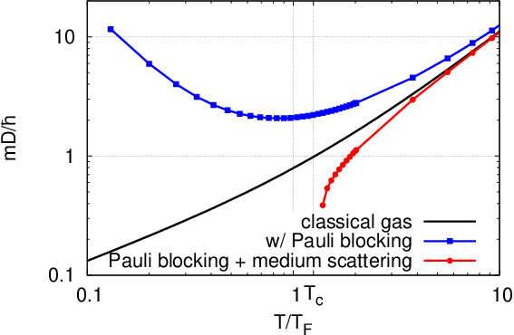
We compute the viscosity of the strongly interacting 2d Fermi gas with full medium effects. The case with Pauli blocking and the bare vacuum scattering cross section, including the limits of high and low temperature, has been discussed in Refs. [28, 29, 30]. Our main finding is that the medium increases scattering for strong interaction and thereby substantially lowers the transport coefficients, see Fig. 1. For vacuum scattering (squares) the system always appears to be in the normal Fermi liquid phase and the upturn of the viscosity for low temperatures is due to Pauli blocking. With medium scattering the viscosity decreases down to a finite temperature where the medium -matrix acquires a pole, (Thouless criterion). Below this pole would formally lead to a diverging collision integral and in this approximation. A calculation of the viscosity in the superfluid phase of 3He for found that Pauli blocking and enhanced scattering cancel precisely and approaches a finite value for [10].

In Fig. 2 the ratio of the viscosity to entropy density is compared for different values of the interaction strength. As the binding energy is lowered, as defined by the Thouless criterion is shifted to lower temperatures, indicated by the endpoints of the solid lines (the endpoints are at ). As an estimate, the minimum for is located at around at a value of , only about twice the proposed string theory bound .

IV.2 Spin diffusion
Equivalently, we have carried out the analysis for the spin diffusion coefficient . In the high-temperature limit [29]
| (34) |
the diffusion coefficient depends linearly on with logarithmic corrections, see Fig. 3. Pauli blocking (squares) increases diffusion, while the inclusion of medium effects leads to a strong reduction of the diffusion coefficient (circles).
V Comparison to experiment
In order to compare our results for the balanced homogeneous 2d Fermi gas with experiments in a trap we perform an average over the density profile of the trap assuming the local density approximation to hold. At high temperatures the density profile in the trap is [28]
| (35) |
with , radial trapping frequency and total density . The local Fermi temperature is given in terms of the density as
| (36) |
such that the local reduced temperature is
| (37) |
and the local pressure of the free Fermi gas is, cf. (33),
| (38) |
The frequency dependent shear viscosity of the homogeneous system is in kinetic theory [44, 28, 15]
| (39) |
in accordance with the viscosity sum rule [45]. From the dimensionless ratio one obtains the viscous scattering time
| (40) |
The local viscosity can be defined in terms of the local reduced temperature ,
| (41) |
The spatial integral of the viscosity diverges at because the dc viscosity is density independent in the outer regions of the trap [28, 29]. In order to obtain a finite integral the viscosity is evaluated at the quadrupole frequency [27],
| (42) |
The global Fermi temperature allows us to define a global reduced temperature , so that the trap averaged viscosity can be written as
| (43) |
with dimensionless pressure . We can change variables and integrate ,
| (44) |
Finally, the quadrupole damping rate is [27]
| (45) |
with for the density profile in Eq. (35). In the high-temperature limit the integrals can be solved analytically and yield [28]
| (46) | ||||
| (47) | ||||
| (48) |
where we have used and . In Fig. 4 we show the quadrupole damping rate vs. interaction strength and compare with the experimental values [27]. The effect of the medium scattering is most pronounced at low temperature and strong interaction. This leads to strongly enhanced damping, and the peak height agrees well with experiment, while previous theoretical studies found lower peak values [29, 30]. Still, the peak position in our calculation occurs at a larger interaction parameter than in the experiment.

VI Conclusion
We have investigated the temperature dependence of the shear viscosity and spin diffusion in a two-component Fermi gas in two dimensions with contact interactions. We used the Boltzmann equation where in contrast to former works we took the medium effect due to finite fermion density into account. We show that the proper inclusion of this effect leads to strong suppression of both transport quantities. Performing the trap average we find that the inclusion of medium effects quantitatively brings us rather close to the experimental findings [27]. It is an important question for the future to confirm the result obtained within the Boltzmann framework with a more refined calculation which does not rely on the validity of the quasiparticle picture and possibly extends below .
Acknowledgements.
We acknowledge discussions with M. Köhl, R. Schmidt and W. Zwerger, and we thank M. Köhl for sending us data. LF acknowledges related collaborations and many discussions with J. Lux, M. Müller, J. Schmalian, and S. Sachdev. This work was supported by the “Deutsche Forschungsgemeinschaft” within SFB 608 (LF), the Bonn-Cologne Graduate School (CK), and the Emmy-Noether Program Grant No. FR 2627/3-1 (CK, LF).
References
- [1] I. Bloch, J. Dalibard, and W. Zwerger, Rev. Mod. Phys. 80, 885 (2008).
- [2] G. Policastro, D. T. Son, and A. O. Starinets, Phys. Rev. Lett. 87, 081601 (2001).
- [3] P. K. Kovtun, D. T. Son, and A. O. Starinets, Phys. Rev. Lett. 94, 111601 (2005).
- [4] T. Schäfer and D. Teaney, Rep. Prog. Phys. 72, 126001 (2009).
- [5] M. Müller, J. Schmalian, and L. Fritz, Phys. Rev. Lett. 103, 025301 (2009).
- [6] A. Turlapov, J. Kinast, B. Clancy, L. Luo, J. Joseph, and J. E. Thomas, J. Low Temp. Phys. 150, 567 (2008).
- [7] C. Cao, E. Elliott, J. Joseph, H. Wu, J. Petricka, T. Schäfer, and J. E. Thomas, Science 331, 58 (2011).
- [8] C. Cao, E. Elliott, H. Wu, and J. E. Thomas, New J. Phys. 13, 075007 (2011).
- [9] L. D. Landau and I. M. Khalatnikov, Zh. Eksp. Teor. Fiz. 19, 637 and 709 (1949), English translation in Collected Papers of L. D. Landau (Pergamon Press, Oxford, 1965), p. 494.
- [10] C. J. Pethick, H. Smith, and P. Bhattacharyya, Phys. Rev. Lett. 34, 643 (1975).
- [11] G. Rupak and T. Schäfer, Phys. Rev. A 76, 053607 (2007).
- [12] P. Massignan, G. M. Bruun, and H. Smith, Phys. Rev. A 71, 033607 (2005).
- [13] G. M. Bruun and H. Smith, Phys. Rev. A 72, 043605 (2005).
- [14] S. Riedl, E. R. Sanchez Guajardo, C. Kohstall, A. Altmeyer, M. J. Wright, J. Hecker Denschlag, R. Grimm, G. M. Bruun, and H. Smith, Phys. Rev. A 78, 053609 (2008).
- [15] T. Enss, Phys. Rev. A 86, 013616 (2012).
- [16] G. M. Bruun and H. Smith, Phys. Rev. A 75, 043612 (2007).
- [17] T. Enss, R. Haussmann, and W. Zwerger, Ann. Phys. (N.Y.) 326, 770 (2011).
- [18] G. Wlazłowski, P. Magierski, and J. E. Drut, arXiv:1204.0270 [Phys. Rev. Lett. (to be published)].
- [19] A. Sommer, M. Ku, G. Roati, and M. W. Zwierlein, Nature (London) 472, 201 (2011).
- [20] A. Sommer, M. Ku, and M. W. Zwierlein, New J. Phys. 13, 055009 (2011).
- [21] G. M. Bruun, New J. Phys. 13, 035005 (2011).
- [22] B. Fröhlich, M. Feld, E. Vogt, M. Koschorreck, W. Zwerger, and M. Köhl, Phys. Rev. Lett. 106, 105301 (2011).
- [23] R. Schmidt, T. Enss, V. Pietilä, and E. Demler, Phys. Rev. A 85, 021602(R) (2012).
- [24] P. Dyke, E. D. Kuhnle, S. Whitlock, H. Hu, M. Mark, S. Hoinka, M. Lingham, P. Hannaford, and C. J. Vale, Phys. Rev. Lett. 106, 105304 (2011).
- [25] A. T. Sommer, L. W. Cheuk, M. J. H. Ku, W. S. Bakr, and M. W. Zwierlein, Phys. Rev. Lett. 108, 045302 (2012).
- [26] M. Koschorreck, D. Pertot, E. Vogt, B. Fröhlich, M. Feld, and M. Köhl, Nature (London) 485, 619 (2012).
- [27] E. Vogt, M. Feld, B. Fröhlich, D. Pertot, M. Koschorreck, and M. Köhl, Phys. Rev. Lett. 108, 070404 (2012).
- [28] T. Schäfer, Phys. Rev. A 85, 033623 (2012).
- [29] G. M. Bruun, Phys. Rev. A 85, 013636 (2012).
- [30] L. Wu and Y. Zhang, Phys. Rev. A 85, 045601 (2012).
- [31] R. Schmidt and T. Enss, Phys. Rev. A 83, 063620 (2011).
- [32] S. K. Adhikari, Am. J. Phys. 54, 362 (1986).
- [33] M. Randeria, J.-M. Duan, and L.-Y. Shieh, Phys. Rev. Lett. 62, 981 (1989).
- [34] L. D. Landau and E. M. Lifshitz, Quantum Mechanics (Butterworth-Heinemann, Oxford, 1981).
- [35] J. Hofmann, Phys. Rev. A 84, 043603 (2011).
- [36] C. Langmack, M. Barth, W. Zwerger, and E. Braaten, Phys. Rev. Lett. 108, 060402 (2012).
- [37] P. Nozieres and S. Schmitt-Rink, J. Low Temp. Phys. 59, 195 (1985).
- [38] J. R. Engelbrecht and M. Randeria, Phys. Rev. Lett. 65, 1032 (1990).
- [39] J. R. Engelbrecht and M. Randeria, Phys. Rev. B 45, 12419 (1992).
- [40] J. M. Ziman, Electrons and Phonons (Oxford University Press, Oxford, 1960).
- [41] H. Smith and H. H. Jensen, Transport phenomena (Oxford University Press, New York, 1989).
- [42] P. Arnold, G. D. Moore, and L. G. Yaffe, J. High Energy Phys. 11, 001 (2000).
- [43] M. Müller and H. C. Nguyen, New J. Phys. 13, 035009 (2011).
- [44] M. Braby, J. Chao, and T. Schäfer, New J. Phys. 13, 035014 (2011).
- [45] E. Taylor and M. Randeria, arXiv:1205.1525.