A narrow $DNN$ quasi-bound state

We consider seven (eight) coupled channels in the isospin $I=0$ ($I=1$) sector, $DN$, $\pi\Sigma_{c}$, $\eta\Lambda_{c}$, $K\Xi_{c}$, $K\Xi_{c}^{\prime}$, $D_{s}\Lambda$, and $\eta^{\prime}\Lambda_{c}$ ($DN$, $\pi\Lambda_{c}$, $\pi\Sigma_{c}$, $\eta\Sigma_{c}$, $K\Xi_{c}$, $K\Xi_{c}^{\prime}$, $D_{s}\Sigma$, and $\eta^{\prime}\Sigma_{c}$). In Ref. [39], the coupled-channel interaction is given by the Weinberg-Tomozawa term

$$v_{ij}^{(I)}(W)=-\frac{\kappa C_{ij}^{(I)}}{4f^{2}}(2W-M_{i}-M_{j})\sqrt{\frac{M_{i}+E_{i}}{2M_{i}}}\sqrt{\frac{M_{j}+E_{j}}{2M_{j}}},$$

where $W$ is the total energy, $f$ is the meson decay constant, $M_{i}$ and $E_{i}$ are the mass and energy of the baryon in channel $i$, respectively, and $C_{ij}^{(I)}$ is the group theoretical coupling strength for isospin $I$. The reduction factor $\kappa$ is introduced to take into account the mass difference of the exchanged meson, which we set $\kappa=1$ ($\kappa=\kappa_{c}=1/4$) for the $uds$ (charm) flavor exchange process [39]. The scattering amplitude $t_{ij}$ is obtained from the matrix equation

$$t^{(I)}=((v^{(I)})^{-1}-g^{(I)})^{-1},$$

(1)

where the diagonal loop function is given in dimensional regularization as

		$\displaystyle g_{i}^{(I)}(W;a_{i}(\mu))$
	$\displaystyle=$	$\displaystyle\frac{1}{(4\pi)^{2}}\Bigl\{a_{i}(\mu)+\ln\frac{M_{i}^{2}}{\mu^{2}}+\frac{m_{i}^{2}-M_{i}^{2}+W^{2}}{2W^{2}}\ln\frac{m_{i}^{2}}{M_{i}^{2}}$
		$\displaystyle+\frac{\bar{q}_{i}}{W}[\ln(W^{2}-(M_{i}^{2}-m_{i}^{2})+2W\bar{q}_{i})$
		$\displaystyle+\ln(W^{2}+(M_{i}^{2}-m_{i}^{2})+2W\bar{q}_{i})$
		$\displaystyle-\ln(-W^{2}+(M_{i}^{2}-m_{i}^{2})+2W\bar{q}_{i})$
		$\displaystyle-\ln(-W^{2}-(M_{i}^{2}-m_{i}^{2})+2W\bar{q}_{i})]\Bigr\},$

where $\bar{q}_{i}$ is the magnitude of the three-momentum in the center-of-mass frame. We choose the subtraction constants at $\mu=1$ GeV as

$\displaystyle a_{DN}=$

$\displaystyle-2.056,\quad a_{i}=-2.06\ (i\neq DN),$

(2)

for both the $I=0$ and $I=1$ states, so that the $\Lambda_{c}(2595)$ resonance is dynamically generated at the observed energy. By choosing the isospin symmetric subtraction constants (2), a resonance state is also generated in $I=1$ at $\sim 2760$ MeV. The diagonal components of the $s$-wave scattering amplitudes in the $DN$ channel, which are complex above the $\pi Y_{c}$ ($Y_{c}=\Lambda_{c},\Sigma_{c}$) threshold, are shown in Fig. 1. The resonant nature of the amplitudes can be seen in both channels.

It is worth comparing the $I=0$ $DN$-$\pi\Sigma_{c}$ system with the corresponding $\bar{K}N$-$\pi\Sigma$ system. Both the systems have a quasi-bound state. Neglecting the small effect of the normalization factor, we can write the coupling strength for the $DN$ case as

$\displaystyle v_{ij}\sim$

$\displaystyle\begin{pmatrix}3&\sqrt{\frac{3}{2}}\kappa_{c}\\ \sqrt{\frac{3}{2}}\kappa_{c}&4\\ \end{pmatrix}\frac{2W-M_{i}-M_{j}}{4f^{2}},$

where the channels are assigned as $DN$ ($i=1$) and $\pi\Sigma_{c}$ ($i=2$). This is the same form with the $\bar{K}N$-$\pi\Sigma$ case, except for the factor $\kappa_{c}=1/4$ in the off-diagonal channel. The diagonal interaction is proportional to the meson energy $W-M_{i}$, which is reduced to the meson mass at threshold. Thus, there are three differences from the strangeness sector: 1) heavy mass of $D$ meson, which enhances the strength of the $DN$ interaction by the energy factor $W-M_{i}$; 2) large reduced mass of the system, which suppresses the kinetic energy in the charm sector; 3) weak transition coupling $DN\to\pi\Sigma_{c}$, which suppresses the decay of the quasi-bound state into the $\pi\Sigma_{c}$ state. These facts explain the reason why the $DN$ quasi-bound state is generated with larger binding energy and narrower width than those of the $\bar{K}N$ quasi-bound state. In addition, 1) and 2) also enhance the attractive interaction in the $I=1$ channel. As a consequence, we obtain a resonance state also in $I=1$ at $\sim 2760$ MeV, as far as choosing the isospin symmetric subtraction constants (2).

Now we construct an effective single-channel potential, which will be used in the variational calculation of the $DNN$ system. We utilize the method in Ref. [45], first constructing a single-channel framework which is equivalent to Eq. (1) and then translating the result into a local and energy-dependent potential in coordinate space.

The effective interaction $v^{\text{eff}}$ is constructed to reproduce the original amplitude $t_{11}$, given by the $DN$ single-channel scattering equation (we suppress the isospin index in this section)

$\displaystyle t_{11}=$

$\displaystyle[(v^{\text{eff}})^{-1}-g_{1}]^{-1}.$

(3)

It is shown that the $v^{\text{eff}}$ is given by the sum of the bare interaction in channel 1 $(v_{11})$ and the term with coupled-channel effects as [45]

$\displaystyle v^{\text{eff}}=$

$\displaystyle v_{11}+\sum_{m=2}^{N}v_{1m}g_{m}v_{m1}+\sum_{m,l=2}^{N}v_{1m}g_{m}t^{(N-1)}_{ml}g_{l}v_{l1},$

(4)

where $t^{(N-1)}_{ml}=[(v^{(N-1)})]^{-1}-g^{(N-1)}]^{-1}$ is the $(N-1)\times(N-1)$ matrix of the coupled-channel amplitude without the $DN$ channel. In this way, Eq. (3) gives the equivalent amplitude with the $11$ component in Eq. (1). $v^{\text{eff}}$ is complex above the $\pi Y_{c}$ threshold, because of the imaginary part of the loop function of the $\pi Y_{c}$ channel in Eq. (4).

We then translate $v^{\text{eff}}$ into the local potential in coordinate space. Adopting a single gaussian form for the spatial distribution, the two-body potential can be written as

	$\displaystyle v_{DN}(r;W)=$	$\displaystyle\frac{M_{N}}{2\pi^{3/2}a_{s}^{3}\tilde{\omega}(W)}$
		$\displaystyle\times[v^{\text{eff}}(W)+\Delta v(W)]\exp[-(r/a_{s})^{2}],\quad$		(5)

where $a_{s}=0.4$ fm is the range parameter of the potential and $\tilde{\omega}(W)$ is the reduced energy of the $DN$ system. The energy-dependent correction term $\Delta v(W)$ is introduced to compensate the deviation from the local potential approximation. This complex and energy-dependent potential reproduces the scattering amplitude $t_{11}$ when the Schrödinger equation with this potential is self-consistently solved. The strength of the potential $v_{DN}(r;W)$ at $r=0$ is shown in Fig. 2. One finds that the real part (imaginary part) is larger (smaller) than that of the $\bar{K}N$ potential [45], which demonstrate the differences of the interaction kernel discussed in the previous section.

In the FCA to the Faddeev equations for the $DNN$ three body system, one takes the $NN$ as a cluster and $D$ scatters from that cluster. We consider the $DNN$ system with total isospin $I_{\text{tot}}=1/2$ and with the total spin-parity $J^{P}=0^{-}$ and $J^{P}=1^{-}$. In this approach, all the two-body pairs are in $s$ wave.

First we make the evaluation for the case of $J^{P}=0^{-}$, which corresponds to the spin (isospin) of the $NN$ pair as $S_{NN}=0$ $(I_{NN}=1)$. To have total isospin $I_{\text{tot}}=1/2$, the dominant component of the $DN$ system is $I=0$, where the $\Lambda(2595)$ resonance appears.

The $T$ matrix for the three-body $DNN$ scattering is labeled by the $DN$ isospins in the entrance channel $I$ and the exit channel $I^{\prime}$, $T_{I,I^{\prime}}$. We denote the two-body ($s$-wave) $DN$ scattering amplitudes by $t^{(0)}$ for $I=0$ and $t^{(1)}$ for $I=1$. Then the $T$ matrix satisfies

$\displaystyle T_{I,I^{\prime}}=t^{(I)}\delta_{I,I^{\prime}}+t^{(I)}G_{I,I^{\prime\prime}}G_{0}T_{I^{\prime\prime},I^{\prime}}P_{ex},$

(6)

which is diagrammatically represented in Fig. 3. In Eq. (6), $G_{0}$ is the meson exchange propagator [58, 34]

$$G_{0}=\int\frac{d^{3}q}{(2\pi)^{3}}F_{NN}(q)\frac{1}{{q^{0}}^{2}-\vec{q}\,^{2}-m_{D}^{2}+i\epsilon},$$

(7)

where $F_{NN}(q)$ is the form factor, representing momentum distribution of the $NN$ system. $P_{ex}$ is the isospin exchange factor, which depends on the total isospin of the nucleon, $I_{NN}$, in the final state, $P_{ex}=(-1)^{I_{NN}+1}=1$ for $J=0$, and $=-1$ for $J=1$.

Here we concentrate on the isospin factors in the $DNN$ scattering amplitudes. We define the isospin doublets, $N=(p,n)$, $D=(D^{+},-D^{0})$ and consider the $DNN$ states with the total isospin $I_{\text{tot}}=1/2$. There are two independent states with the total spin $J=0$ and $J=1$, which can be decomposed into the $DN$ isospin eigenstates, as

	$\displaystyle|D(N_{1}N_{2})_{I_{NN}=1}\rangle_{J=0}=\frac{\sqrt{3}}{2}|(DN_{1})_{0}N_{2}\rangle+\frac{1}{2}|(DN_{1})_{1}N_{2}\rangle,$
	$\displaystyle|D(N_{1}N_{2})_{I_{NN}=0}\rangle_{J=1}=-\frac{1}{2}|(DN_{1})_{0}N_{2}\rangle+\frac{\sqrt{3}}{2}|(DN_{1})_{1}N_{2}\rangle.$

The $D$ exchange matrix is given in terms of the isospin recombination factors.

	$\displaystyle|(DN_{1})_{0}N_{2}\rangle=\frac{1}{2}|(DN_{2})_{0}N_{1}\rangle+\frac{\sqrt{3}}{2}|(DN_{2})_{1}N_{1}\rangle,$
	$\displaystyle|(DN_{1})_{1}N_{2}\rangle=\frac{\sqrt{3}}{2}|(DN_{2})_{0}N_{1}\rangle-\frac{1}{2}|(DN_{2})_{1}N_{1}\rangle.$

Thus the transition matrix $G$ is given by

$\displaystyle G=\begin{pmatrix}\displaystyle\frac{1}{2}&\displaystyle\frac{\sqrt{3}}{2}\\ \displaystyle\frac{\sqrt{3}}{2}&-\displaystyle\frac{1}{2}\end{pmatrix}.$

The three-body amplitude $T_{I,I^{\prime}}$ is obtained by solving Eq. (6):

	$\displaystyle T=$	$\displaystyle\left[1-\frac{1}{2}(t^{(0)}-t^{(1)})G_{0}P_{ex}-t^{(0)}t^{(1)}G_{0}^{2}\right]^{-1}$
		$\displaystyle\times\begin{pmatrix}t^{(0)}+\frac{1}{2}t^{(1)}G_{0}t^{(0)}P_{ex}&\frac{\sqrt{3}}{2}t^{(0)}t^{(1)}G_{0}P_{ex}\\ \frac{\sqrt{3}}{2}t^{(0)}t^{(1)}G_{0}P_{ex}&t^{(1)}-\frac{1}{2}t^{(0)}G_{0}t^{(1)}P_{ex}\end{pmatrix}.$

In calculating the $T$ matrix for the scatterings in the $J=0$ and $J=1$ channels, we take the linear combinations, with a factor 2 for the choice of the first nucleon, as

	$\displaystyle T(J=0)=2\begin{pmatrix}\frac{\sqrt{3}}{2}&\frac{1}{2}\end{pmatrix}\begin{pmatrix}T_{00}&T_{01}\\ T_{10}&T_{11}\end{pmatrix}\begin{pmatrix}\frac{\sqrt{3}}{2}\\ \frac{1}{2}\end{pmatrix},$
	$\displaystyle T(J=1)=2\begin{pmatrix}-\frac{1}{2}&\frac{\sqrt{3}}{2}\end{pmatrix}\begin{pmatrix}T_{00}&T_{01}\\ T_{10}&T_{11}\end{pmatrix}\begin{pmatrix}-\frac{1}{2}\\ \frac{\sqrt{3}}{2}\end{pmatrix}.$

Substituting the $T$ matrix and replacing $P_{ex}$ by $+1$ for $J=0,I_{NN}=1$ scattering and $-1$ for $J=1,I_{NN}=0$, we obtain

	$\displaystyle T(J=0)=$	$\displaystyle\left(\frac{3}{2}t^{(0)}+\frac{1}{2}t^{(1)}+2t^{(0)}t^{(1)}G_{0}\right)$
		$\displaystyle\times\left[1-\frac{1}{2}(t^{(0)}-t^{(1)})G_{0}-t^{(0)}t^{(1)}G_{0}^{2}\right]^{-1},$		(8)
	$\displaystyle T(J=1)=$	$\displaystyle\left(\frac{1}{2}t^{(0)}+\frac{3}{2}t^{(1)}+2t^{(0)}t^{(1)}G_{0}\right)$
		$\displaystyle\times\left[1+\frac{1}{2}(t^{(0)}-t^{(1)})G_{0}-t^{(0)}t^{(1)}G_{0}^{2}\right]^{-1}.$		(9)

These results coincide with those derived in the charge basis [35, 36] (see Appendix B).

We can see that Eq. (7) contains the folding of the $D$ intermediate propagator with the form factor of the $NN$ system. The variable $q^{0}$ in Eq. (7) is the energy carried by the $D$, which is given by

$$q^{0}=\frac{s+m_{D}^{2}-(2M_{N})^{2}}{2\sqrt{s}},$$

with $\sqrt{s}$ for the rest energy of the $DNN$ system. Eq. (7) requires the $NN$ form factor. For $I_{NN}=0$ one could take the deuteron form factor, but the attraction of the $D$ on the nucleons will make the $NN$ system more compact, like in the case of the $\bar{K}NN$ system. Yet, there are limits on how much one can contract this system because of the strong $NN$ repulsion at short distances. In order to estimate the $NN$ size one can rely upon the results of Ref. [30] in the study of the $\bar{K}NN$ system, where the $NN$ repulsion at short distance was explicitly taken into account. In practical terms we use the same expression for the form factor as for the deuteron [59]

$\displaystyle F(q)=\int^{\infty}_{0}d^{3}p~\sum_{j=1}^{11}\frac{C_{j}}{\vec{p}^{2}+m_{j}^{2}}\sum_{i=1}^{11}\frac{C_{i}}{(\vec{p}-\vec{q})^{2}+m_{i}^{2}},$

(10)

but with the parameters $m_{i}$ rescaled such as to give an average separation of the nucleons of $R_{NN}\simeq 2$ fm [30]. They are shown in Fig. 4. The validity of this $NN$ form factor will be examined by the result of the variational calculation, where the average distance of the $NN$ pair in the $DNN$ system will be optimized in the three-body dynamics.

We need the argument $s_{1}$ of the $DN$ amplitude, $t(\sqrt{s_{1}})$. To evaluate it we adopt a common procedure of dividing the binding energy into the three particles proportionally to their masses. The energy of the nucleon and the $D$ meson are given by

$$E_{N}=M_{N}\frac{\sqrt{s}}{2M_{N}+m_{D}}~,~E_{D}=m_{D}\frac{\sqrt{s}}{2M_{N}+m_{D}},$$

so the total energy of the two-body system can be calculated as

$$s_{1}=(p_{D}+p_{N_{1}})^{2}=s~\Big(\frac{M_{N}+m_{D}}{2M_{N}+m_{D}}\Big)^{2}-\vec{p}_{N_{2}}^{~2}.$$

(11)

The approximate value of $\vec{p}_{N_{2}}^{2}$ can be obtained by assuming

$$\frac{\vec{p}_{N_{2}}^{~2}}{2M_{N}}\simeq B_{N_{2}};~~B_{N_{2}}=M_{N}-M_{N}\frac{\sqrt{s}}{2M_{N}+m_{D}},$$

(12)

which provides a rough estimate for bound systems with the strong interaction.

As we shall see in Sec. V, we obtain a $DNN$ bound system with a very small width. This is related to the small width of the $\Lambda_{c}(2598)$ state which is generated in $DN$ interaction in $I=0$. Yet, this calculation only takes into account the decay channel $DN\rightarrow\pi\Sigma_{c}$ for which there is little phase space and $DN\rightarrow\pi\Lambda_{c}$ channel which comes from the subdominant $DN$ $I=1$ component in the $DNN$ system. Now we allow the $D$ to be absorbed by two nucleons, in analogy to the $\bar{K}NN\rightarrow\Lambda N$ considered in Refs. [11, 44]. Here the channel will be $DNN\rightarrow N\Lambda_{c}$ whose absorption process is shown diagrammatically in Fig. 5 (other mechanisms and decay channels will be discussed in the end of this section). We calculate only the first diagram in Fig. 5. The second one gives an identical contribution and they sum incoherently: there is no interference since the $N\Lambda_{c}$ and $\Lambda_{c}N$ are orthogonal states. Hence, the total width will be twice the one obtained from just one diagram.

The $S$-matrix for the diagram is given by

	$\displaystyle S$	$\displaystyle=$	$\displaystyle\int d^{4}x\int d^{4}y(-i)t_{DN\rightarrow DN}$
			$\displaystyle\times\frac{1}{\sqrt{2\omega_{D}}}\varphi_{D}(\vec{x})e^{-i\omega_{D}x^{0}}e^{iE^{\prime}_{N_{1}}x^{0}}e^{-iE_{N_{1}}x^{0}}\varphi^{*}_{N^{\prime}_{1}}(\vec{x})\varphi_{N_{1}}(\vec{x})$
			$\displaystyle\times\int\frac{d^{4}q}{(2\pi)^{4}}e^{-iq(y-x)}\frac{i}{q^{2}-m_{D}^{2}+i\epsilon}$
			$\displaystyle\times V_{y}\vec{\sigma}\vec{q}~e^{iE_{\Lambda_{c}}y^{0}}e^{-iE_{N_{2}}y^{0}}\varphi^{*}_{\Lambda_{c}}(\vec{y})\varphi_{N_{2}}(\vec{y}),$

where $V_{y}$ is the Yukawa vertex. We take the same coupling as $K^{-}p\rightarrow\Lambda$ since in the $D$ and $\Lambda_{c}$ the $c$ quark plays the role of the $s$ quark in the ${\bar{K}}$ and $\Lambda$. In Ref. [60], the $V_{y}$ is given as

$\displaystyle V_{y}=-\frac{1}{\sqrt{3}}\frac{3F+D}{2f},$

with $D=0.795$, $F=0.465$ [61]. We perform the $x^{0}$, $y^{0}$ integrations, and make a change of the spatial variables as

$\displaystyle\vec{x}=\vec{R}-\frac{\vec{r}}{2},\quad\vec{y}=\vec{R}+\frac{\vec{r}}{2}.$

Then we can write

$\displaystyle\varphi_{N_{1}}(\vec{x})\varphi_{N_{2}}(\vec{y})=\frac{1}{\sqrt{V}}e^{i\vec{P}.\vec{R}}\varphi(\vec{r}),$

where $\varphi(\vec{r})$ is the wave function of the $NN$ system. $N^{\prime}_{1}$ and $\Lambda_{c}$ will be outgoing plane waves. Let us also assume that the $D$ is a plane wave with a certain momentum. The final formula that we shall use is independent of this momentum, as we shall see. Thus,

$\displaystyle\varphi_{D}(\vec{x})=\frac{1}{\sqrt{V}}e^{i\vec{p}_{D}.\vec{x}},$

and then, using these new functions, the $S$-matrix is written as follows

	$\displaystyle S$	$\displaystyle=$	$\displaystyle\frac{1}{V^{2}}\int\frac{d^{3}q}{(2\pi)^{3}}\frac{1}{\sqrt{2\omega_{D}}}t_{DN\rightarrow DN}\frac{1}{q^{2}-m_{D}^{2}+i\epsilon}~$		(13)
			$\displaystyle\times V_{y}\vec{\sigma}\vec{q}~\tilde{\varphi}(\vec{q}-\vec{p}_{\Lambda_{c}}+\frac{\vec{P}}{2})(2\pi)^{4}\delta^{4}(p_{i}-p_{f})$
		$\displaystyle\equiv$	$\displaystyle-iT\frac{1}{\sqrt{2\omega_{D}}}\frac{1}{V^{2}}(2\pi)^{4}\delta^{4}(p_{i}-p_{f}),$

where $\tilde{\varphi}(\vec{q})$ is the Fourier transform of the wave function $\varphi(\vec{r})$ normalized to 1, and $p_{i}$ and $p_{f}$ are the initial and final momentum, respectively. The $NN$ wave function in momentum space is defined as

$$\tilde{\varphi}(\vec{q})=\int d^{3}qe^{i\vec{q~}\vec{x}}\varphi(\vec{x}),$$

and has a maximum value for $\vec{q}=0$. If we take the $NN$ system at rest, $\vec{P}=0$, the wave function $\tilde{\varphi}(\vec{q})$ in Eq. (13) will peak at $\vec{q}-\vec{p}_{\Lambda_{c}}=0$. This allows us to approximate the $D$ propagator in Eq. (13) as

$\displaystyle\frac{1}{q^{2}-m_{D}^{2}}\rightarrow\frac{1}{(q^{0})^{2}-\vec{p}^{~2}_{\Lambda_{c}}-m_{D}^{2}},$

(14)

where $q^{0}=E_{\Lambda_{c}}-E_{N_{2}}$ and $p_{\Lambda_{c}}\approx\lambda^{1/2}(M_{NND}^{2},M_{N}^{2},M_{\Lambda_{c}}^{2})/2M_{NND}$. We do not need to specify the $t_{DN\rightarrow DN}$ amplitude since it will be accounted for at the end of the formalism.

Defining of $\vec{q}-\vec{p}_{\Lambda_{c}}\equiv\vec{q}~^{\prime}$, the square of the total matrix element is obtained as follow:

	$\displaystyle|T|^{2}$	$\displaystyle=$	$\displaystyle V_{y}^{2}\vec{p}^{~2}_{\Lambda_{c}}\left(\frac{1}{(q^{0})^{2}-p_{\Lambda_{c}}^{2}-m_{D}^{2}}\right)^{2}$		(15)
			$\displaystyle\times\left|\frac{1}{2\pi^{2}}\int q^{\prime 2}dq^{\prime}\tilde{\varphi}(\vec{q}~^{\prime})t_{DN,DN}(\sqrt{s^{\prime}})\right|^{2},$

With this $T$ matrix we evaluate the cross section for the process of Fig. 5 (left) and we obtain

$\displaystyle\sigma_{\text{abs}}=\frac{1}{2\pi}\frac{M_{NN}M_{\Lambda_{c}}M_{N}}{M_{NND}^{2}}\frac{p_{\Lambda_{c}}}{p_{D}}|T|^{2}.$

It is interesting to relate this cross section to the imaginary part of the forward $D(NN)\rightarrow D(NN)$ amplitude from the diagram of Fig. 6 using the optical theorem. We find

$\displaystyle\text{Im }T_{D(NN)}=-\frac{p_{D}\sqrt{s}}{M_{NN}}\sigma_{\text{abs}}=-\frac{1}{2\pi}\frac{M_{\Lambda_{c}}M_{N}}{M_{NND}}p_{\Lambda_{c}}|T|^{2}.$

The next step is to convert the absorption diagram of the Fig. 6 (a) into a “many body” diagram of Fig. 6 (b) where the nucleon where the $D$ is absorbed, the only occupied state of the “many body” system, is converted into a hole state in the many body terminology [62]. Once this is done one observes that if we remove the amplitude $t_{DN}$ in the expression of $T$, the expression that we obtain for $\text{Im }T_{D(NN)}$ corresponds to the evaluation of the imaginary part of the two-body loop function $g$ of a nucleon and a $D$ meson [Fig. 6 (c)] but with a $D$ selfenergy insertion accounting for the ($\Lambda_{c}N_{h}$) excitation of the $D$ meson. We call this $\delta\tilde{g}$. The Feynman rules to evaluate $\text{Im }\delta\tilde{g}$ and $\text{Im }T_{D(NN)}$ are identical, except that $t_{DN,DN}$ is removed in the evaluation of $\text{Im }\delta\tilde{g}$. Hence we obtain

$\displaystyle i\text{Im }\delta\tilde{g}=-i\frac{1}{2\pi}\frac{M_{\Lambda_{c}}M_{N}}{M_{NND}}p_{\Lambda_{c}}|\tilde{T}|^{2}.$

with $|\tilde{T}|^{2}$ is given by Eq. (15) removing $t_{DN,DN}$. This simplifies the expression since

	$\displaystyle\frac{1}{2\pi^{2}}\int q^{\prime 2}dq^{\prime}\tilde{\varphi}(\vec{q}~^{\prime})=$	$\displaystyle\lim_{r\rightarrow 0}\int\dfrac{d^{3}q^{\prime}}{(2\pi)^{3}}e^{i\vec{q}~^{\prime}\vec{r}}\tilde{\varphi}(\vec{q}~^{\prime})$		(16)
	$\displaystyle=$	$\displaystyle\varphi(r=0).$

Thus $|\tilde{T}|^{2}$ is given by

$\displaystyle|\tilde{T}|^{2}$

$\displaystyle=$

$\displaystyle V_{y}^{2}\vec{p}^{~2}_{\Lambda_{c}}\frac{1}{[(q^{0})^{2}-p_{\Lambda_{c}}^{2}-m_{D}^{2}]^{2}}|\varphi(0)|^{2}.$

Finally $\vec{p}^{~2}_{\Lambda_{c}}$ accompanying $V_{y}^{2}$ in the former expression requires a small correction. The factor comes from the non relativistic $\vec{\sigma}\vec{q}$ form of the $DN\Lambda_{c}$ vertex. If we take instead the relativistic Yukawa vertex of the type $\gamma^{\mu}\gamma^{5}$, then we find the easy prescription to account for the relativistic correction,

$\displaystyle V_{y}^{2}\vec{p}^{~2}_{\Lambda_{c}}$

$\displaystyle\rightarrow$

$\displaystyle V_{y}^{2}\frac{1}{4m_{\Lambda_{c}}^{2}}(M_{N}+M_{\Lambda_{c}})^{2}\vec{p}^{~2}_{\Lambda_{c}}.$

The next step is to reevaluate the $t_{DN,DN}$ amplitude used as input in the fixed center formulas. As we mentioned, they were obtained using the method of Ref. [39] with several coupled channels and the formula (1). We redo the evaluation by replacing the loop function in the $DN$ channel as

$$g_{DN}\rightarrow g_{DN}+i~\text{Im }\delta\tilde{g}$$

(17)

to take into account the $D$ absorption by two nucleons or, analogously, the $\Lambda_{c}N_{h}$ excitation of the $D$ meson. When doing this, the $DN$ amplitude becomes complex below the $DN$ threshold and the narrow $\Lambda_{c}(2598)$ resonance acquires now a moderate width due to the $D$ absorption with a second nucleon. The second process of Fig. 5 (right) is accounted for when we consider the three-body amplitude $T$ in the FCA formula with the first $D$ scattering with the second nucleon.

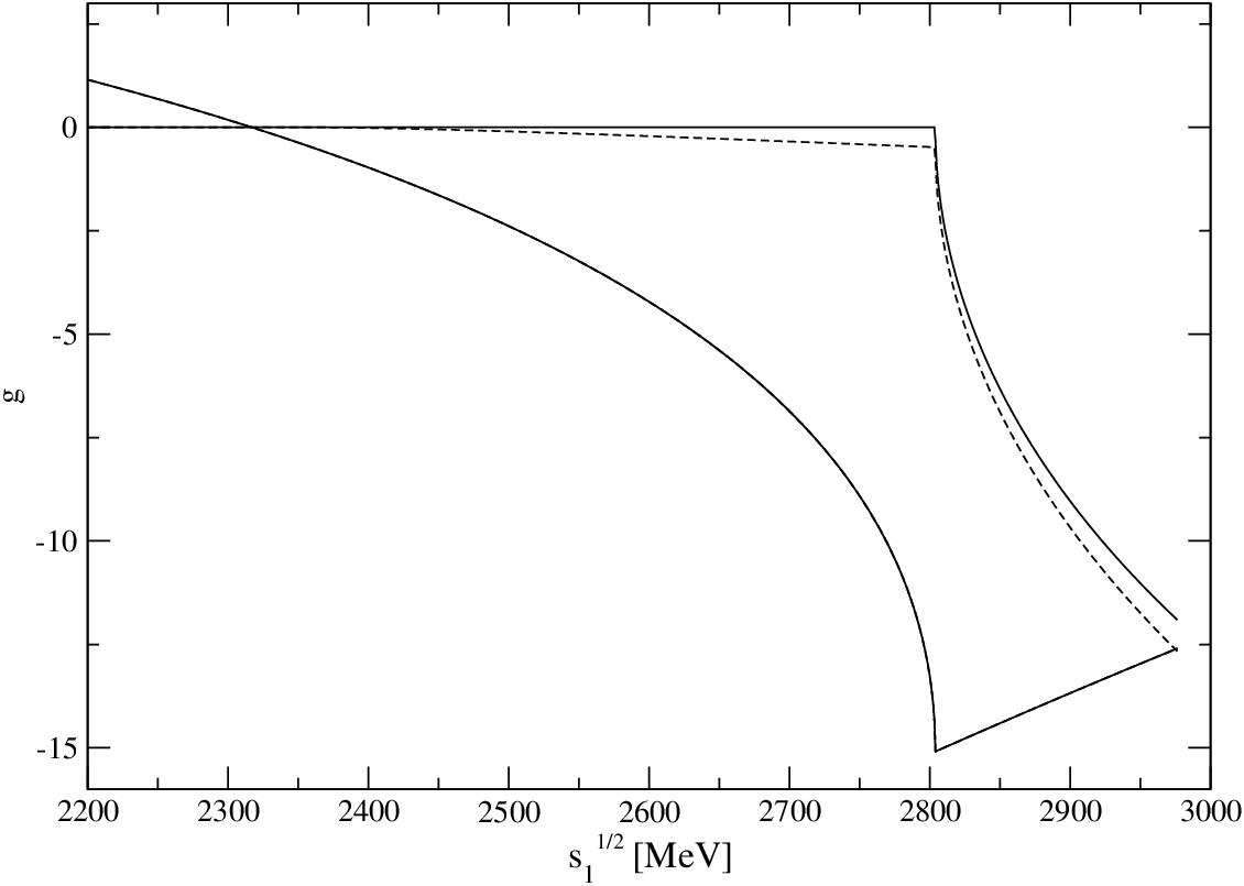
For the estimation of the width we take the wave function

	$\displaystyle\tilde{\varphi}(r)=$	$\displaystyle ae^{-\alpha r},\quad a=\frac{1}{2}\left(\frac{\alpha^{3}}{2\pi}\right)^{\frac{1}{2}},$
	$\displaystyle\tilde{\varphi}(q)=$	$\displaystyle\frac{4\pi a\alpha}{(\frac{1}{4}\alpha^{2}-q^{2})^{2}+q^{2}\alpha^{2}},$

with $\alpha\simeq 1.7\text{fm}^{-1}$, which corresponds to an $NN$ object of relative distance $2\,\text{fm}$.

Let us numerically investigate the effect of the absorption using the model described in Sec. II.1. In Fig. 7, we show the meson-baryon loop function $g_{DN}$ in the $DN$ channel together with the two-body absorption contribution to the imaginary part, $i\text{Im }\delta\tilde{g}$. We can see that the imaginary part of the total $g$ function is no longer zero below the $DN$ threshold due to $D$ absorption. In Fig. 8, we show the modulus of the two-body amplitude $|t|$ for the $DN$ channel for $I=0$ using $g_{DN}$ and $g_{DN}+i\text{Im }\delta\tilde{g}$ of Eq. (17). As we can see, the inclusion of the absorption mechanism induces an increase in the width of the peak of $\Lambda_{c}(2595)$ in $|t|$ which will have repercussion in the width of the $DNN$ system.

For a narrow resonance, we can approximate the amplitude around the resonance energy by a Breit-Wigner form

$$t(\sqrt{s_{1}})\simeq\dfrac{g^{2}}{\sqrt{s_{1}}-M_{R}+i\frac{\Gamma}{2}}.$$

This leads to the expression of the coupling of the resonance to the $DN$ scattering state as

$$g^{2}=\frac{1}{2}\Gamma|t(M_{R})|.$$

Inspection of Fig. 8, together with the values of $\Gamma$(no absorption)$=$ 3 MeV and $\Gamma$(absorption)$=$ 15 MeV, show that the value of the coupling $g^{2}$ barely changes from the introduction of $i\text{Im }\delta\tilde{g}$, but of course the resonance has become wider. Indeed $g^{2}$(no absorption)/ $g^{2}$(absorption)$\simeq 6/5$.

The absorption diagram that we have considered is not the only one, but it is the most relevant. On the same footing we should consider the diagrams where the Yukawa coupling produces $\Sigma_{c}$ or even $\Sigma^{*}_{c}(2520)$. The analogy with the kaons made before, and the values of these couplings that can be seen in Ref. [61], together with the dynamical factor $p^{3}$ of the cross section, make the contribution of these terms of the order of 5% of the $\Lambda_{c}$ production and we neglect them. Analogously we can also have $DN\to\pi(\eta)\Lambda_{c}(\Sigma_{c})$ in the first hadron line of the absorption diagram and exchange a pion or an eta. These diagrams are further suppressed because they require the exchange of a heavy vector in the $DN\to\pi(\eta)Y_{c}$ amplitude in the extension of the hidden gauge approach that we use. They are penalized by the factor $\kappa_{c}^{2}$, which, even considering that the pion (eta) propagators have bigger strength than the $D$ one, renders these diagrams at the level of 10%.

References

- [1] M. Krell, T. E. O. Ericson, Nucl. Phys. B11, 521-550 (1969).
- [2] H. Toki, S. Hirenzaki, T. Yamazaki, R. S. Hayano, Nucl. Phys. A501, 653 (1989).
- [3] J. Nieves, E. Oset, C. Garcia-Recio, Nucl. Phys. A554, 509-553 (1993).
- [4] C. J. Batty, E. Friedman, A. Gal, Phys. Rept. 287, 385-445 (1997).
- [5] S. Hirenzaki, Y. Okumura, H. Toki, E. Oset, A. Ramos, Phys. Rev. C61, 055205 (2000).
- [6] R. S. Hayano, T. Hatsuda, Rev. Mod. Phys. 82, 2949 (2010).
- [7] S. Hirenzaki, H. Toki, T. Yamazaki, Phys. Rev. C44, 2472-2479 (1991).
- [8] J. Nieves, E. Oset, Phys. Lett. B282, 24-30 (1992).
- [9] K. J. Raywood, J. B. Lange, G. Jones, M. Pavan, M. E. Sevior, D. A. Hutcheon, A. Olin, D. Ottewell et al., Phys. Rev. C55, 2492-2500 (1997).
- [10] M. Lutz, Phys. Lett. B426, 12-20 (1998).
- [11] A. Ramos, E. Oset, Nucl. Phys. A671, 481-502 (2000).
- [12] J. Schaffner-Bielich, V. Koch, M. Effenberger, Nucl. Phys. A669, 153-172 (2000).
- [13] A. Cieply, E. Friedman, A. Gal, J. Mares, Nucl. Phys. A696, 173-193 (2001).
- [14] E. Friedman, A. Gal, C. J. Batty, Nucl. Phys. A579, 518-538 (1994).
- [15] A. Baca, C. Garcia-Recio, J. Nieves, Nucl. Phys. A673, 335-353 (2000).
- [16] V. K. Magas, E. Oset, A. Ramos, H. Toki, Phys. Rev. C74, 025206 (2006).
- [17] E. Oset, V. K. Magas, A. Ramos, H. Toki, On the 9th International Conference On Hypernuclear And Strange Particle Physics (HYP 2006), 10-14 Oct 2006, Mainz, Germany.
- [18] R. H. Dalitz and S. F. Tuan, Phys. Rev. Lett. 2, 425 (1959); Annals Phys. 10, 307 (1960).
- [19] N. Kaiser, P. B. Siegel, and W. Weise, Nucl. Phys. A594, 325 (1995).
- [20] E. Oset and A. Ramos, Nucl. Phys. A635, 99 (1998).
- [21] J. A. Oller and U. G. Meissner, Phys. Lett. B500, 263 (2001).
- [22] M. F. M. Lutz and E. E. Kolomeitsev, Nucl. Phys. A700, 193 (2002).
- [23] D. Jido, J. A. Oller, E. Oset, A. Ramos, U. G. Meissner, Nucl. Phys. A725, 181-200 (2003).
- [24] T. Hyodo and D. Jido, Prog. Part. Nucl. Phys. 67, 55 (2012), 1104.4474.
- [25] Y. Ikeda, T. Hyodo and W. Weise, Phys. Lett. B 706, 63 (2011); Nucl. Phys. A, 881, 98 (2012).
- [26] Y. Ikeda and T. Sato, Phys. Rev. C 76, 035203 (2007).
- [27] N. V. Shevchenko, A. Gal and J. Mares, Phys. Rev. Lett. 98, 082301 (2007).
- [28] N. V. Shevchenko, A. Gal, J. Mares and J. Revai, Phys. Rev. C 76, 044004 (2007).
- [29] A. Dote, T. Hyodo and W. Weise, Nucl. Phys. A 804, 197 (2008).
- [30] A. Dote, T. Hyodo and W. Weise, Phys. Rev. C 79, 014003 (2009).
- [31] Y. Ikeda and T. Sato, Phys. Rev. C 79, 035201 (2009).
- [32] T. Yamazaki and Y. Akaishi, Phys. Lett. B 535 (2002) 70.
- [33] Y. Ikeda, H. Kamano, T. Sato, Prog. Theor. Phys. 124, 533-539 (2010).
- [34] M. Bayar, J. Yamagata-Sekihara, E. Oset, Phys. Rev. C84, 015209 (2011).
- [35] E. Oset, D. Jido, T. Sekihara, A. M. Torres, K. P. Khemchandani, M. Bayar and J. Yamagata-Sekihara, Nucl. Phys. A 881, 127 (2012).
- [36] M. Bayar and E. Oset, arXiv:1203.5313 [nucl-th].
- [37] N. Barnea, A. Gal and E. Z. Liverts, arXiv:1203.5234 [nucl-th].
- [38] J. Hofmann, M. F. M. Lutz, Nucl. Phys. A763, 90-139 (2005).
- [39] T. Mizutani, A. Ramos, Phys. Rev. C74, 065201 (2006).
- [40] L. Tolos, A. Ramos, T. Mizutani, Phys. Rev. C77, 015207 (2008).
- [41] C. Garcia-Recio, V. K. Magas, T. Mizutani, J. Nieves, A. Ramos, L. L. Salcedo, L. Tolos, Phys. Rev. D79, 054004 (2009).
- [42] L. Tolos, C. Garcia-Recio, J. Nieves, Phys. Rev. C80, 065202 (2009).
- [43] C. Garcia-Recio, J. Nieves, L. Tolos, Phys. Lett. B690, 369-375 (2010).
- [44] T. Sekihara, D. Jido, Y. Kanada-En’yo, Phys. Rev. C79, 062201 (2009).
- [45] T. Hyodo and W. Weise, Phys. Rev. C 77, 035204 (2008).
- [46] R. Chand, R. H. Dalitz, Annals Phys. 20, 1-19 (1962).
- [47] G. Toker, A. Gal, J. M. Eisenberg, Nucl. Phys. A362, 405-430 (1981).
- [48] S. S. Kamalov, E. Oset, A. Ramos, Nucl. Phys. A690, 494-508 (2001).
- [49] U. -G. Meissner, U. Raha, A. Rusetsky, Eur. Phys. J. C47, 473-480 (2006).
- [50] A. Gal, Int. J. Mod. Phys. A22, 226-233 (2007).
- [51] J. -J. Xie, A. Martinez Torres, E. Oset, Phys. Rev. C83, 065207 (2011).
- [52] D. Jido, Y. Kanada-En’yo, Phys. Rev. C78, 035203 (2008).
- [53] A. Martinez Torres, K. P. Khemchandani, E. Oset, Phys. Rev. C79, 065207 (2009).
- [54] A. Martinez Torres, D. Jido, Phys. Rev. C82, 038202 (2010).
- [55] J. -J. Xie, A. Martinez Torres, E. Oset, P. Gonzalez, Phys. Rev. C83, 055204 (2011).
- [56] C. W. Xiao, M. Bayar, E. Oset, Phys. Rev. D84, 034037 (2011).
- [57] A. Martinez Torres, E. J. Garzon, E. Oset, L. R. Dai, Phys. Rev. D83, 116002 (2011).
- [58] L. Roca and E. Oset, Phys. Rev. D 82, 054013 (2010).
- [59] R. Machleidt, Phys. Rev. C 63, 024001 (2001).
- [60] E. Oset, A. Ramos, Nucl. Phys. A679, 616-628 (2001).
- [61] B. Borasoy, Phys. Rev. D59, 054021 (1999).
- [62] A. L. Fetter, J. D. Walencka, Quantum Theory of Many-particle Systems, McGRAW-HILL, 1971.
- [63] A. Hasegawa and S. Nagata, Prog. Theor. Phys. 45, 1786 (1971).
- [64] D. R. Thompson, M. Lemere, and Y. C. Tang, Nucl. Phys. A286, 53 (1977).
- [65] R. B. Wiringa, V. G. J. Stoks, and R. Schiavilla, Phys. Rev. C51, 38 (1995).
- [66] T. Yamazaki and Y. Akaishi, Phys. Rev. C76, 045201 (2007).
- [67] A. Arai, M. Oka, and S. Yasui, Prog. Theor. Phys. 119, 103 (2008).
- [68] T. Uchino, T. Hyodo, and M. Oka, Nucl. Phys. A868-869, 53 (2011).
- [69] A. B. Kaidalov, P. E. Volkovitsky, Z. Phys. C63, 517-524 (1994).
- [70] A. Khodjamirian, C. .Klein, T. .Mannel, Y. -M. Wang, Eur. Phys. J. A 48, 31 (2012).
- [71] U. Wiedner, Prog. Part. Nucl. Phys. 66, 477-518 (2011).
- [72] S. Cho et al. [ExHIC Collaboration], Phys. Rev. Lett. 106, 212001 (2011).
- [73] S. Cho et al. [ExHIC Collaboration], Phys. Rev. C 84, 064910 (2011).