Microwave spectroscopy of a Cooper pair beam splitter
Abstract
This article discusses how to demonstrate the entanglement of the split Cooper pairs produced in a double-quantum-dot based Cooper pair beam splitter (CPS), by performing the microwave spectroscopy of the CPS. More precisely, one can study the DC current response of such a CPS to two on-phase microwave gate irradiations applied to the two CPS dots. Some of the current peaks caused by the microwaves show a strongly nonmonotonic variation with the amplitude of the irradiation applied individually to one dot. This effect is directly due to a subradiance property caused by the coherence of the split pairs. Using realistic parameters, one finds that this effect has a measurable amplitude.
pacs
73.23.-b,73.63.Fg,03.67.BgI I. Introduction
Quantum entanglement between spatially separated particles represents a promising resource in the field of quantum computation and communication. However, this fascinating behavior can be difficult to observe in practice due to decoherence caused by the particles environment. This is why the ”spooky action at a distance” was first demonstrated with photons, atoms, or ions which can be naturally placed in weakly interacting conditions[1, 2, 3].
Observing electronic entanglement in solid state systems is a-priori more challenging since an electronic fluid is characterized by a complex many-body state in general. However, quantum entanglement has been recently observed on superconducting chips[4]. In this case, the particles are replaced by superconducting quantum bits, which can be sufficiently well isolated from the outside world thanks to the rigidity of the superconducting phase, if an appropriate circuit design is used. In these experiments, the entangled degrees of freedom are defined from the charges of small superconducting islands, or from the persistent current states of a superconducting loop, for instance[5].
Superconductors enclose another natural source of entanglement which has not been exploited so far, i.e. the spin entanglement of its Cooper pairs. In a conventional superconductor, Cooper pairs gather two electrons correlated in a spin-singlet state. The use of this resource for entanglement production requires to build hybrid circuits in which the superconductors are connected to non-superconducting elements which allow the spatial separation of Cooper pairs. In principle, a double quantum dot circuit connected to a central superconducting contact (input) and two outer normal metal contacts (outputs) facilitates this process[6]. Such a ”Cooper pair splitter” (CPS) has been realized recently by using double dots formed inside semiconducting nanowires [7, 8, 9] or carbon nanotubes[10, 11]. The spatial splitting of the Cooper pairs has been demonstrated from an analysis of the current response of the CPS to a DC voltage bias. However, the spin entanglement of the split pairs was not tested by these experiments.
It has been suggested to use the noise cross-correlations of the electrical current to characterize the degree of entanglement of pairs of electrons[12, 13, 14, 15, 16, 17, 18, 19, 20, 21]. Alternatively, Ref. [22] proposes to put in evidence spin entanglement by coupling the CPS to a microwave cavity. In this reference, a double quantum dot formed inside a single wall carbon nanotube is considered. Spin-orbit interaction produces a coupling between electronic spins and cavity photons. Such a coupling leads to a lasing effect which involves a transition between the spin singlet state in which Cooper pairs are injected and some spin triplet states. This effect vanishes when the spin/photon coupling is equal in the two dots, due to a subradiance property caused by the entangled structure of the spin-singlets. However, realizing such an experimental scheme is challenging since it requires to couple a complex quantum dot circuit to a photonic cavity[23, 24, 25].
The present work suggests an alternative strategy to exploit the subradiance of spin-orbit induced transitions between spin singlet and spin triplet CPS states. One can measure the DC current at the input of the CPS when microwave gate voltage excitations are applied separately to the two CPS dots. The microwave-induced state transitions mediated by spin-orbit coupling result in current peaks at the input of the CPS versus the dots DC gate voltages. Assuming that two on-phase microwave excitations are applied to the two dots, these peaks vanish when the amplitude of the two excitations become equal. This subradiant behavior is directly related to the spin-entanglement of the split Cooper pairs hosted by the CPS.
This article is organized as follows. Section II defines the CPS hamiltonian, for a single wall carbon nanotube based implementation. Section III discusses the CPS even-charged eigenstates in the absence of the microwave excitations and without the normal metal contacts. Section IV describes the coupling between the CPS even-charged eigenstates and the microwave excitations. Section V describes the CPS state dynamics in the presence of the voltage-biased normal metal contacts, by using a master equation description. Section VI describes the results given by this approach, an in particular the predictions obtained for the DC current at the input of the CPS. Section VII presents further examination and modifications of the model, which are useful to put the results of section VI into perspective. In particular, it discusses the role of atomic-scale disorder in the nanotube, the role of the form assumed for the spin-orbit interaction term, and possible microwave induced transitions in the CPS singly occupied charge sector. Section VIII compares the measurement strategy discussed in this work to the one of Ref. [22]. Section IX concludes. Although this article focuses on a carbon-nanotube-based CPS, the entanglement detection scheme discussed in this work could be generalized to other types of quantum dots with spin-orbit coupling like e.g. InAs quantum dots, in principle.
II II. Hamiltonian of the CPS
Let us consider the circuit represented schematically in Fig. 1. Two normal metal contacts and a superconducting contact are used to define two quantum dots and along a single wall carbon nanotube. The superconducting contact is connected to ground, and a bias voltage is applied to the two normal metal contacts. The dot is connected capacitively to a DC gate voltage source and a microwave gate voltage source . In the following, it is assumed that and are in-phase, i.e. .

Inside the left and right dots , an electron with spin can be in the orbital of the nanotube, which is reminiscent from the degeneracy of graphene. One can use a double dot hamiltonian which takes into account the proximity effect caused by the superconducting contact, i.e.
| (1) | ||||
with
| (2) |
the creation operator for an electron with spin in orbital of dot and . For simplicity, one can assume that the orbital energies in dots and are both equal to in the absence of the external microwave irradiation, which can be obtained by tuning properly the dots’ DC gate voltages . The term is caused by spin-orbit coupling inside the carbon nanotube[26]. The term describes a coupling between the and orbitals of dot , due to disorder at the level of the nanotube atomic structure [27, 28, 26, 29]. The term in describes interdot hopping. The term accounts for Coulomb charging effects. One can assume that there cannot be more than one electron in each dot, due to a strong intra-dot Coulomb charging energy. Therefore, Cooper pairs injected inside the CPS are split into two electrons, one in each dot. The term accounts for coherent injection of singlet Cooper pairs inside the double dot [30]. This approach is valid provided quasiparticle transport between the superconducting contact and the double dot can be disregarded. This requires , with the BCS gap of the superconducting contact. The hamiltonian must be supplemented by the normal leads hamiltonian
| (3) |
and the tunnel coupling between the dots and normal leads
| (4) |
with the annihilation operator for an electron with spin in orbital of the normal lead .
The effect of the microwave gate voltage bias can also be described with hamiltonian terms. The gate voltage corresponds to an electric field , with the center to ground separation of the waveguide providing the microwave signal. This also corresponds in the Coulomb gauge to a vector potential on dot , which is assumed to be perpendicular to the carbon nanotube. The interplay between and intersubband spin-orbit coupling elements induced by the nanotube curvature results in a spin/photon coupling term (see Ref. [31] for details)
| (5) |
with the electron charge. For simplicity, this article uses the particular structure with and the imaginary unit number, obtained from a microscopic description of spin-orbit coupling in a zigzag nanotube quantum dot [31], based on Refs.[32, 33] (see also Refs. 34, 35, 36, 38, 37). However, part VII.1 will show that the results presented here can be generalized straightforwardly to a more general . The dimensionless coefficient corresponds to the coefficient of reference [22], with the amplitude of vacuum voltage fluctuations for the photonic cavity considered in this reference. The value of can be estimated to typically while can reach typically . One can also use a hamiltonian term to account for the modulation of the dots orbital energies by the microwave gate voltages. For simplicity, one can disregard the mutual capacitive coupling between the two dots. In this case, one finds
| (6) |
where is a dimensionless capacitive coupling constant which is typically of the order of .
In the following, it is assumed that electrons can go from dot to the corresponding normal metal contact but not the reverse. This can be obtained by using a bias voltage such that
| (7) |
with and a dimensionless coefficient which takes into account the effective thermal broadening of the levels (see Ref. [31] for details).
III III. Expression of the even-charged CPS eigenstates
This section discusses the relevant eigenstates of in the even charge sector for , with the energy of a CPS doubly occupied state for . The parameter can be tuned with .

The coupling hybridizes the CPS empty state with the subspace of the CPS doubly occupied states {}, where denotes a CPS state with one electron with spin in orbital of dot L and one electron with spin in orbital of dot R [39, 40]. The resulting even-charged subspace is called . Near the working point , the CPS dynamics involves a subspace of at maximum five eigenstates from . Three of these eigenstates have an energy , namely
| (8) | ||||
| (9) | ||||
and
| (10) | ||||
where denotes the spin direction opposite to and . The two remaining eigenstates
| (11) |
and
| (12) |
have eigenenergies
| (13) |
with
| (14) | ||||
and
| (15) |
The existence of the degree of freedom complicates slightly the definition of the CPS eigenstates. However, from the definition of , one can see that corresponds to a generalized spin-singlet state whereas , and correspond to generalized spin-triplet states. The coupling hybridizes the empty state with only, due to the hypothesis that the superconducting contact injects spin-singlet pairs inside the CPS. Figure 2.a shows the energies , and as a function of . The energies and show an anticrossing with a width at , due to the coherent coupling between and . The energy of the triplet states lies between and . Figure 2.b shows the transition frequencies , and of the CPS, with . These frequencies will play an important role in the following.
IV IV. Microwave-induced matrix elements
This section discusses the effect of the microwave gate bias on the eigenstates defined in section III. Inside the subspace , has only three finite matrix elements, i.e.
| (16) | ||||
and
| (17) |
These terms are finite because flips the spins in the dots. The minus sign in Eq.(16) is a direct consequence of the fact that comprises a singlet component whereas is a triplet state. In contrast, the plus sign in Eq.(17) is due to the fact that and are both triplet states. The matrix element of Eq.(17) is always non-resonant since it couples two states with the same energy. Therefore, it can be disregarded in our study. The hamiltonian has only one finite coupling element in the subspace , i.e.
| (18) |
with . The addition of and in Eq. (18) is due to the fact that the double occupation energy is shifted by when a microwave excitation is applied to the device.
One can find experimental means to have and on phase, in agreement with the assumption made in section II. In this case, the matrix element vanishes when . This effect is directly related to the injection of coherent singlet Cooper pairs inside the CPS since it is due to the existence of the minus sign in Eq. (16). If the injected pairs were in a product state instead of an entangled state, the matrix element (16) would not be subradiant (see section VII.4). Therefore, coherent pair injection inside the CPS can be revealed by observing microwave-induced transitions between and , and checking that these transitions are suppressed for . The following sections describe how to probe these microwave-induced transitions with a DC current measurement.
V V. Master equation description of the CPS dynamics
In the following, the states and are disregarded because they are not populated in simple limits where relaxation towards them is neglected. The sequential tunneling limit is furthermore assumed, with the tunnel escape rate of an electron from one of the dots to the corresponding normal lead. For simplicity, it is assumed that this rate does not depend on the dot orbital and spin indices. This would change only quantitatively the results shown in this paper. In the absence of microwave irradiation, the dynamics of the CPS can be described with a master equation[30, 41]
| (19) |
with
| (20) |
and
| (21) |
Above, denotes the probability of state , with . The vector also includes the global probability of having a double dot singly occupied state. The use of this global probability is sufficient to describe the dynamics of the CPS because the single electron tunnel rate to the normal leads is assumed to be independent from the dot orbital and spin indices. The various singly occupied eigenstates of are defined in section VII.3. The exact relation has been used to simplify the above expression of .
The microwave excitation can induce resonances between the states and while the excitation couples and . One can use a rotating frame approximation on independent resonances to describe these effects. This approach is valid provided one of the microwave-induced resonance has a dominant effect on the others, which requires the frequencies , and to be sufficiently different. The rotating frame approximation also requires to use small amplitudes and compared to , , and . In this case, the stationary state occupation probabilities can be obtained from
| (22) |
with
| (23) | ||||
| (28) |
| (29) | ||||
| (30) | ||||
| (31) |
and . Above, corresponds to the coherence time between the states and . Assuming that is limited by tunneling to the normal leads, one obtains , and .
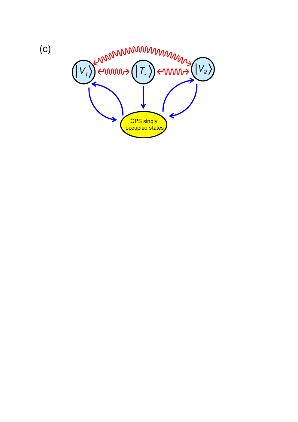
Figure 2.c represents schematically the dynamics of the CPS near the working point . Due to the assumptions made in section II on , the tunnel transitions between the different CPS states (blue arrows) always occur together with the transfer of one electron towards one of the normal metal contacts. In contrast, the microwave irradiation induces transitions between the states and , and , or and without any exchange of electrons with the normal contacts (red wavy arrows). The state can be reached through a microwave-induced transition but not through a tunnel process because it has no component in . The states and can be both reached or left through a tunnel event because they have components in both and .
VI VI. Results
VI.1 VI.1 Principle of the measurement
From Eq. (21), the tunnel rate transitions from the states , , and to the ensemble of the singly occupied states are , and respectively, while the tunnel transition rate from a singly occupied state to or is . As a result, the DC current flowing at the input of the CPS can be calculated as
| (32) |
with . Figure 3.a shows the coefficients and as a function of . One can conclude from this plot that except at , the various components of have different values. Therefore, a microwave excitation changing the population of the states , , and should affect the value of the DC current flowing through the CPS. This effect will be used in the following to reveal the microwave-induced transitions between , , and .
VI.2 VI.2 Stationary CPS state occupations
Let us first discuss the dependence of the CPS state probabilities on the parameter for (see Fig.3, black dotted lines in the three lowest panels). To understand this dependence, one must keep in mind the fact that the tunnel rate transitions from the states and to the ensemble of the singly occupied states are and , as already discussed in section VI.1. For well below , tends to zero. As a result, the CPS cannot escape easily from the state , whose probability tends to 1. This is because in this limit, the state is almost equal to the empty state , which makes the emission of an electron towards the normal leads very difficult. On opposite, for well above , it is the probability of the state which tends to one because tends to . In the absence of a microwave irradiation, the probability of state remains equal to zero since transitions towards these state are not possible.

Let us now discuss the case finite (see Fig. 3, red full lines in the three lowest panels). The term excites the transition, which causes peaks or dips in and for , i.e. with
| (33) |
The term excites the and transitions, which causes peaks in for and , i.e. and respectively, with
| (34) |
and
| (35) |
The term also causes peaks or dips in and , but they are hardly visible due to the scale used in Fig. 3. The decoherence rates , and have similar order of magnitudes (between and ). However, the width of the peaks or dips caused by seems much larger than the width of the peaks caused by . This is due to the limit considered here. As long as the different types of resonances are well separated in frequency, the resonance gives probabilities and which tend to the value 1/4 for sufficiently large. In principle, the and resonances give state probabilities which saturate at more complicated values which depend on when and become sufficiently large. In the regime considered here, the resonance is saturated while the and resonances are only weakly excited. This explains that the width of the peaks or dips related to the resonance are much larger.
VI.3 VI.3 Average current at the input of the CPS
It is useful to discuss first the value of the current at the input of the CPS in the absence of the microwave excitations. The current can be obtained from Eq.(32) with . From Fig. 4.a, shows a maximum for , where the two states and both correspond to equally weighted superpositions of and . For well below or well above , the current vanishes because the CPS is blocked in the states or , respectively (see section V).
Figure 4.b shows the difference between the current for a finite microwave irradiation and , as a function of and . The transitions yield a broad resonance along the curve , which has a frequency minimum at . However, this resonance vanishes close to because at this point, the tunnel escape rates and of the CPS from and are equal since and therefore, the microwave-induced transitions between the states and cannot be seen anymore through a measurement of . The and resonances yield two thinner resonances which cross at the point corresponding to and . For tending to zero, the ( ) resonance progressively vanishes from because this corresponds to a regime where the state () is not populated anymore. Note that the calculation of the current very close to the point is in principle not valid using the rotating wave approximation on independent resonances since at this point. However, this represents only an extremely small area of Fig. 4.a (of order ). Discussing the behavior of the CPS near point goes beyond the scope of this paper.


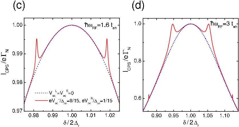
Figures. 4.c and 4.d show as a function of for two different values of . In Fig. 4.c, only the and resonances are visible because . In Fig. 4.d, the resonances are also visible. The and resonances appear as much thinner an smaller peaks. At the resonances, for the parameters used in Fig.4.d, reaches the saturation value expected for large and well separated resonances. This value can be obtained from Eq.(32), using .
VI.4 VI.4 Dependence of the CPS input current on the amplitude of the microwave irradiation
This section discusses how the minus sign in Equation (16) can be seen experimentally. One can note , and the amplitudes of the microwave-induced current peaks appearing for , , and . Due to the symmetries of our model around the point , one has and . The top and bottom panels of Fig. 5 show the variations of and with for a constant value of . Due to the plus sign in Eq. (18), increases monotonically with . In Fig.5, this variation is very small because the resonance is already saturated at due to the value used for . In contrast, due to the minus sign in Eq. (16), shows a minimum for . Note that if the electrons pairs injected in the CPS were not in an entangled state but in a product state, such a non-monotonic behavior would not be possible. For the parameters considered in Fig.5, top panel, vanishes at because the effects of the resonance can be disregarded. This should not be true anymore in the case where the different types of resonances are not well separated, which can happen e.g. if is too small with respect to the width of the resonances. However, in this case, one can still expect to show a strongly non-monotonic behavior with a minimum at , provided the couplings are sufficiently strong. Treating this case requires to go beyond the rotating frame approximation with independent resonances used in this work.

VI.5 VI.5 Experimental parameters
This section discusses the parameters used in the Figs. and the order of magnitude of the signals which can be expected in practice. In Figs. 3 to 5, the ratio of parameters used correspond for instance to realistic values (see Refs. [7, 8, 9, 10, 11]), , and M (see Refs. [27, 28, 26]). Note that M corresponds to mK, therefore the sequential tunneling approximation used in this work is valid using for instance mK. In this case, using , the condition (7) to have electrons flowing only from the dot to the leads and not the reverse gives (see section II). This is compatible with the condition for having no quasiparticle transport between the superconducting lead and the dots, by using for instance a Nb contact for which or a NbN contact for which . Using the above parameters, the ratio used in Figs. 3 and 4 corresponds to realistic microwave amplitudes and . Besides, the maximum frequency considered in this work (see Fig. 4.b) corresponds to , and the frequency at point O corresponds to, which is accessible with current microwave technologies[42]. Using the above parameters, the amplitude of the current peaks and shown in Fig. 3.d are and over a background of and respectively. The maximum current difference in Fig.5, top panel, corresponds to for a background of . Therefore, the features described in this article seem measurable experimentally.
VII VII. Discussion on the spectroscopic entanglement detection scheme
The present section presents further examination and modifications of the model used above, in order to put the results of section VI into perspective.
VII.1 VII.1 Use of a more general spin/orbit coupling term
The coupling term of Eq.(5) accounts for the coupling between the CPS and microwave excitations mediated by spin-orbit coupling. The above sections have used the particular form with , obtained from a microscopic description of spin-orbit coupling in a zigzag nanotube quantum dot[31]. This section discusses the generalization of the results to a more general coupling . Since must be hermitian, one can use and without any loss of generality. The parameter
| (36) |
with plays a crucial role in this case. It is convenient to redefine the states and more generally as
| (37) |
and
| (38) |
with
| (39) | ||||
Note that and are still eigenstates of the hamiltonian , with energy , corresponding to generalized spin triplet states. The definitions of the other states and remain unchanged. Using expressions (37) and (38), one obtains
| (40) |
and
| (41) | ||||
for . In sections II to VI, one uses thus and which is in agreement with Eqs.(9) and (10). In this limit, Eq. (41) agrees with Eq. (16). Equations (41) and (36) show that even with a more general coupling term , the matrix elements still present a subradiant form. Hence, the entanglement detection scheme discussed in this article appears to be quite general. Using a more general will modify only quantitatively the predictions of section VI.
VII.2 VII.2 Role of
Remarkably, the subradiant matrix elements (16) and (41) vanish for . The aim of the present section is to show that using a finite does not represent a fundamental constraint to have the subradiance effect. Indeed, can still be coupled to other triplet states outside of the subspace when . This fact is illustrated below, using for simplicity. In this case, is coupled to a single triplet eigenstate of outside the subspace , defined by
| (42) |
with
| (43) |
| (44) |
| (45) |
and
| (46) |
such that
| (47) |
One can check:
| (48) | ||||
For , one finds:
| (49) |
The coupling between and is subradiant since it vanishes for . Nevertheless, for realistic parameters and in particular , the transition frequencies and correspond approximately to , which is too high for current microwave technology. This is why this paper focuses on microwave-induced transitions inside the subspace .
VII.3 VII.3 Microwave-induced transitions inside the singly occupied charge sector
The different eigenstates of in the singly occupied charge sector can be defined as:
| (50) | ||||
| (51) | ||||
| (52) | ||||
and
| (53) | ||||
for . These states have eigenenergies , , , and respectively, with
| (54) |
and
| (55) |
for . The states and can be seen as generalized bonding states and and as generalized antibonding states. This section uses for simplicity. The term couples and to and only, for . Only the transitions correspond to a finite frequency, i.e. . One can check that
| (56) |
whereas
| (57) | ||||
Importantly, the matrix element of Eq.(56) has a subradiant structure. This property is due to the fact that the states and are entangled states with different symmetries, i.e. is an antibonding state which contains some components whereas is a bonding state which contains components. This is analogous to the fact that the elements couple a state with a spin-singlet component to a spin-triplet state . In contrast, the matrix elements of Eq.(57) are not subradiant because they couple two entangled states with similar symmetries, i.e. two bonding or two antibonding states.
Due to the subradiant form of Eq. (56), the transitions can lead to a non-monotonic variation of the CPS input current as a function of e.g. , due to another type of entanglement than the one discussed in section VI. Therefore, in the context of the characterization of split Cooper pairs entanglement, one needs to find a way to discriminate possible current resonances corresponding to the transitions and . In practice, this should be feasible by studying how the different resonance frequencies vary with the DC gate voltages of the two dots. Indeed, does not depend on the parameter , contrarily to and . Therefore, possible current resonances due to transitions should appear as horizontal lines in Fig. 4.b. This effect was nevertheless disregarded in section VI, assuming that is too large to be accessible experimentally. Studying quantitatively the possibility to observe the resonances requires to go beyond the approximation of an electronic tunnel rate to the normal leads which is independent from the dot orbital and spin indices [43].
VII.4 VII.4 Simplified model without the K/K’ degeneracy
It is interesting to discuss a model without the K/K’ degree of freedom to show simply how the subradiance property arises.
VII.4.1 Case of coherent Cooper pair injection
Let us assume that each of the two CPS dots has a single orbital. One can note a CPS doubly occupied state with a spin on dot . In the case of coherent Cooper pair injection, the double quantum dot effective hamiltonian can be written[30]
| (58) | ||||
where still forbids the double occupation of each dot. One uses above with the creation operator for an electron with spin in dot . Let us furthermore assume that there also exists a spin-flip coupling term to the microwave signal, with the form
| (59) |
Such a spin-flip coupling can be due for instance to the magnetic field associated with the microwave irradiation. In practice, this term should have a very weak amplitude, but it is nevertheless discussed here for fundamental purposes.
The term in hybridizes the CPS empty state with the singlet state , so that an anticrossing appears again in the spectrum of the CPS even-charged states. For simplicity, it is asssumed below that the double occupation energy of the CPS is degenerate with the energy of , i.e. . In this case, one can use the orthonormalized basis of eigenstates of (58) in the even charge sector , with
| (60) |
| (61) |
and
| (62) |
The states and have energies and given by . They play the role of the states and of section VI. It is convenient to define and as superpositions of triplet states with equal spins. The states , and have an energy . One can check straigthforwardly that
thus
| (63) |
whereas and . The states are thus coupled by to a single state , with a subradiant matrix element (63). This illustrates the universality of the mechanism discussed in section VI.
VII.4.2 Case of incoherent singlet injection
One can model naïvely the incoherent injection of Cooper pairs inside the CPS by assuming that up spins are always injected inside the left dot and right spins inside the right dot. This requires to replace the hamiltonian (58) by
| (64) | ||||
One can use again for simplicity. In this case, one can define an orthonormalized basis of eigenstates of (64) in the even charge sector, with
| (65) |
| (66) |
| (67) |
and . The role of the states and of section VI is now played by and . The states and have again energies and defined in the previous section, whereas the states , and have an energy . The states and of the previous section are still CPS eigenstates, but it is more convenient to use the eigenstates and to study the effect of . Due to the term in , the states and still form an anticrossing in the energy spectrum of the CPS. Hence, such an anticrossing is not characteristic from the injection of entangled Cooper pairs. The only state of connected to by is , with a matrix element
| (68) |
which is not subradiant, but increases monotonically with and . Therefore, the subradiance property is lost when Cooper pairs are injected inside the CPS in a product state instead of an entangled state. Similar results are expected for a model including the degree of freedom.This illustrates that the subradiance property is a good indication of the injection of entangled Cooper pairs inside the CPS. More sophisticated descriptions of incoherent injection of Cooper pairs into the CPS are beyond the scope of this article.
VIII VIII. Comparison with an alternative setup: the CPS embedded in a microwave cavity
This section compares the experimental scheme proposed in Ref.[22] to the scheme discussed in the present article. Reference [22] suggests to observe the minus sign in Equation (16) by inserting the CPS inside a coplanar microwave cavity to obtain a lasing effect involving the transition. The minus sign in Equation (16) leads to a non-monotonic dependence of the number of photons in the cavity as a function of the coefficients and , which mediate a coupling between the CPS and the electric field conveyed by the cavity. Since this electric field can be considered as constant over the whole CPS area, it is necessary to be able to vary independently from to observe a non-monotonic behavior in the number of photons. This can require to complexify the CPS design, for instance. In the present scheme, such a control on and is not necessary since it is sufficient to vary independently the amplitudes and . This can be naturally achieved by using two independent microwave supplies for the two gates. The advantage of the scheme presented in Ref.[22] is that the signal to be measured is a large photon number which can be obtained by measuring the power spectrum emitted by the cavity. In other words, the scheme of Ref.[22] exploits the fact that the lasing effect provides an intrinsic amplification process for the transitions. In the present scheme, the measurement seems a bit more difficult since the current peaks to be measured are very small. Nevertheless, such current amplitudes are measurable, in principle[42]. Therefore, the scheme presented in this reference could be an interesting alternative approach to demonstrate the coherent injection of singlet Cooper pairs inside a CPS. This scheme furthermore allows to study also the transition, which is not possible with the scheme of Ref. [22].
IX IX. Conclusion
The DC current response of a double-quantum-dot based Cooper pair beam splitter (CPS) to a microwave gate irradiation is a very rich source of information on Cooper pair splitting. In particular, it can reveal the entanglement of spin-singlet Cooper pairs injected inside the CPS. This article illustrates this property for a double quantum dot formed inside a carbon nanotube with typical parameters. If they are spin-entangled, the injected pairs are coupled to other CPS states through some subradiant microwave transitions mediated by spin-orbit coupling. This property can be revealed by applying to the two CPS quantum dots two on-phase microwave gate voltages. The spin-orbit mediated microwave transitions cause DC current resonances at the input of the CPS. The subradiance property manifests in a strongly nonmonotonic variation of these current resonances with the amplitude of the microwave signal applied to one of the two CPS dots. This behavior does not depend on details of the model like the exact form of the spin-orbit interaction term. Similarly, the presence of atomic disorder in the nanotube has to be assumed only for quantitative reasons. More generally, the entanglement detection scheme discussed in this work could be generalized to other types of quantum dots with spin-orbit coupling like e.g. InAs quantum dots, in principle. For simplicity, this article discusses the limit where the intra-dot charging energies are very strong, so that there cannot be two electrons at the same time on the same dot. For smaller charging energies, the efficiency of Cooper pair splitting should be decreased. Nevertheless, if the CPS produces entangled split Cooper pairs with a sufficient rate, the resulting subradiant current peaks should still be observable. Interestingly, the bonding or antibonding single particle states delocalized on the two dots of the CPS can also cause a subradiant current resonance, because they present another type of entanglement. However, in principle, this resonance can easily be discriminated from the subradiant resonances caused by split Cooper pairs, because of a different dependence on the CPS DC gate voltages.
I acknowledge useful discussions with T. Kontos, J. Viennot and A. Levy Yeyati. This work has been financed by the EU-FP7 project SE2ND[271554].
References
- [1] A. Aspect, P. Grangier, and G. Roger, Phys. Rev. Lett. 49, 91 (1982), A. Aspect, J. Dalibard, and G. Roger, Phys. Rev. Lett. 49, 1804 (1982).
- [2] A.Rauschenbeutel, G. Nogues, S. Osnaghi, P. Bertet, M. Brune, J.-M. Raimond, and S. Haroche, Science 288, 2024 (2000).
- [3] C. A. Sackett, D. Kielpinski, B. E. King, C. Langer, V. Meyer, C. J. Myatt, M. Rowe, Q. A. Turchette, W. M. Itano, D. J. Wineland & C. Monroe, Nature 404, 256 (2000).
- [4] M.s Steffen, M. Ansmann, R. C. Bialczak, N. Katz, E. Lucero, R. McDermott, M. Neeley, E. M. Weig, A. N. Cleland and J. M. Martinis, Science 313, 1423 (2006), L. DiCarlo, J. M. Chow, J. M. Gambetta, Lev S. Bishop, B. R. Johnson, D. I. Schuster, J. Majer, A. Blais, L. Frunzio, S. M. Girvin & R. J. Schoelkopf, Nature 460, 240 (2009), M.Neeley, R. C. Bialczak, M. Lenander, E. Lucero, M. Mariantoni, A. D. O’Connell, D. Sank, H. Wang, M. Weides, J. Wenner, Y. Yin, T. Yamamoto, A. N. Cleland and J. M. Martinis, Nature 467, 570 (2010), L. DiCarlo, M. D. Reed, L. Sun, B. R. Johnson, J. M. Chow, J. M. Gambetta, L. Frunzio, S. M. Girvin, M. H. Devoret and R. J. Schoelkopf, Nature 467, 574 (2010), A. Palacios-Laloy, F. Mallet, F. Nguyen, P. Bertet, D. Vion, D. Esteve and A. Korotkov, Nature Phys. 6, 442 (2010).
- [5] J.Q. You, F. Nori, Nature 474, 589 (2011).
- [6] P. Recher, E. V. Sukhorukov, and D. Loss, Phys. Rev. B 63, 165314 (2001).
- [7] L. Hofstetter, S. Csonka, J. Nygard, and C. Schönenberger, Nature 461, 960 (2009).
- [8] L. Hofstetter, S. Csonka, A. Baumgartner, G. Fülöp, S. d’Hollosy, J. Nygård, C. Schönenberger, Phys. Rev. Lett. 107, 136801 (2011).
- [9] J. Schindele, A. Baumgartner, C. Schönenberger, arXiv:1204.5777
- [10] L. G. Herrmann, F. Portier, P. Roche, A. Levy Yeyati, T. Kontos, and C. Strunk, Phys. Rev. Lett. 104, 026801 (2010).
- [11] L. G. Herrmann, P. Burset, W. J. Herrera, F. Portier, P. Roche, C. Strunk, A. Levy Yeyati, T. Kontos, arXiv:1205.1972
- [12] T. Martin, Phys. Lett. A 220, 137 (1996).
- [13] M. P. Anantram, and S. Datta, Phys. Rev. B 53, 16390 (1996).
- [14] G. Burkard, D. Loss, and E. V. Sukhorukov, Phys. Rev. B 61, 16303 (R) (2000).
- [15] G. B. Lesovik, T. Martin, and G. Blatter, Eur. Phys. J. B 24, 287 (2001).
- [16] J. Borlin, W. Belzig, and C. Bruder, Phys. Rev. Lett. 88, 197001 (2002).
- [17] P. Samuelsson, and M. Büttiker, Phys. Rev. Lett. 89, 046601 (2002).
- [18] N. M. Chtchelkatchev, G. Blatter, G. B. Lesovik, and T. Martin, Phys. Rev. B 66, 161320(R) (2002).
- [19] O. Sauret, T. Martin, and D. Feinberg, Phys. Rev. B 72, 024544 (2005).
- [20] D. Chevallier, J. Rech, T. Jonckheere, and T. Martin, Phys. Rev. B 83, 125421 (2011).
- [21] J. Rech, D. Chevallier, T. Jonckheere, T. Martin, arXiv:1109.2476
- [22] A. Cottet, T. Kontos, and A. Levy Yeyati, Phys. Rev. Lett. 108, 166803 (2012).
- [23] M.R. Delbecq, V. Schmitt, F. D. Parmentier, N. Roch, J. J. Viennot, G. Fève, B. Huard, C. Mora, A. Cottet, and T. Kontos, Phys. Rev. Lett. 107, 256804 (2011).
- [24] T. Frey, P. J. Leek, M. Beck, A. Blais, T. Ihn, K. Ensslin, and A. Wallraff, Phys. Rev. Lett. 108, 046807 (2012).
- [25] Z.-L. Xiang, S. Ashhab, J. Q. You, F. Nori, arXiv:1204.2137
- [26] T. S. Jespersen, K. Grove-Rasmussen, J. Paaske, K. Muraki, T. Fujisawa, J. Nygård, and K. Flensberg, Nature Physics 7, 348 (2011).
- [27] W. Liang, M. Bockrath, and H. Park, Phys. Rev. Lett. 88, 126801 (2002).
- [28] F. Kuemmeth, S. Ilani, D. C. Ralph, and P. L. McEuen, Nature 452, 448 (2008).
- [29] A. Pályi and G. Burkard, Phys. Rev. Lett. 106, 086801 (2011).
- [30] J. Eldridge, M. G. Pala, M. Governale, and J. König, Phys. Rev. B 82, 184507 (2010).
- [31] See Supplemental Material of Ref. [22]
- [32] W. Izumida, K. Sato, and R. J. Saito, Phys. Soc. Jpn., 78, 074707 (2009).
- [33] J. Klinovaja, M. J. Schmidt, B. Braunecker, and D. Loss, Phys. Rev. B 84, 085452 (2011).
- [34] D. Huertas-Hernando, F. Guinea, and A. Brataas, Phys. Rev. B, 74, 155426 (2006).
- [35] T. Ando, J. Phys. Soc. Jpn. 69, 1757 (2000).
- [36] A. DeMartino, R. Egger, K. Hallberg, and C. A. Balseiro, Phys. Rev. Lett. 88, 206402 (2002).
- [37] D. V. Bulaev, B. Trauzettel, and D. Loss, Phys. Rev. B 77, 235301 (2008).
- [38] J.-S. Jeong and H.-W. Lee, Phys. Rev. B 80, 075409 (2009).
- [39] P. Recher, Y. V. Nazarov, and L. P. Kouwenhoven, Phys. Rev. Lett. 104, 156802 (2010).
- [40] F. Godschalk, F. Hassler, and Y. V. Nazarov, Phys. Rev. Lett. 107, 073901 (2011).
- [41] O. Sauret, D. Feinberg, and T. Martin, Phys. Rev. B 70, 245313 (2004).
- [42] C. Meyer, J. M. Elzerman, and L. P. Kouwenhoven, Nano Lett., 7, 295, (2007).
- [43] Note that in principle, the term can induce transitions , at the frequency . However, the states and have similar weights in , , , and . Therefore, these transitions should not be visible in the CPS input current.