-body simulations with a cosmic vector for dark energy
Abstract
We present the results of a series of cosmological -body simulations of a Vector Dark Energy (VDE) model, performed using a suitably modified version of the publicly available GADGET-2 code. The setups of our simulations were calibrated pursuing a twofold aim: 1) to analyze the large scale distribution of massive objects and 2) to determine the properties of halo structure in this different framework. We observe that structure formation is enhanced in VDE, since the mass function at high redshift is boosted up to a factor of ten with respect to CDM, possibly alleviating tensions with the observations of massive clusters at high redshifts and early reionization epoch. Significant differences can also be found for the value of the growth factor, that in VDE shows a completely different behaviour, and in the distribution of voids, which in this cosmology are on average smaller and less abundant. We further studied the structure of dark matter haloes more massive than , finding that no substantial difference emerges when comparing spin parameter, shape, triaxiality and profiles of structures evolved under different cosmological pictures. Nevertheless, minor differences can be found in the concentration-mass relation and the two point correlation function; both showing different amplitudes and steeper slopes. Using an additional series of simulations of a CDM scenario with the same and used for the VDE cosmology, we have been able to establish wether the modifications induced in the new cosmological picture were due to the particular nature of the dynamical dark energy used or a straightforward consequence of the cosmological parameters used. On large scales, the dynamical effects of the cosmic vector can be seen in the peculiar evolution of the cluster number density function with redshift, in the distribution of voids and on the characteristic form of the growth index . On smaller scales, internal properties of haloes are almost unaffected by the change of cosmology, since no statistical difference can be observed in the characteristics of halo profiles, spin parameters, shapes and triaxialities. Only halo masses and concentrations show a substantial increase, which can however be attributed to the change in the cosmological parameters.
Keywords:
methods:-body simulations – galaxies: haloes – cosmology: theory – dark matter1 Introduction
During the last twelve years, a large amount of cosmological high precision data on
Supernovae Ia (Riess
et al., 1998; Perlmutter
et al., 1999; Guy
et al., 2010, see)
cosmic microwave background anisotropies (Larson
et al., 2011; Sherwin
et al., 2011),
weak lensing (Huterer, 2010), baryon acoustic oscillations
(Beutler
et al., 2011) and large scale structure surveys (Abazajian
et al., 2009)
has provided evidence that the Universe we live in is of a flat geometry and undergoing an accelerated expansion.
These observations motivate our belief in the existence
of an ubiquitous fluid called dark energy (DE)
that by the exertion of a negative pressure,
counters and eventually overcomes the gravitational attraction
that would otherwise dominate the evolution of our Universe.
The simplest explanation to the nature of this fluid
is found in the standard model of cosmology
CDM, where the role of the DE is played by a cosmological constant
obeying the equation of state .
Although perfectly consistent with all the aforementioned observations, CDM still
lacks of appeal from a purely theoretical point of view.
In fact, if we belive the cosmological constant to be the zero point energy
of some fundamental quantum field,
its introduction in the Friedmann equations requires
a fine-tuning of several tens of orders of magnitude
(depending on the energy scale we choose to be fundamental in our theory)
spoiling the naturalness of the whole CDM picture.
Another issue we encounter when dealing with the standard cosmological
model is the so called coincidence problem, that is,
the difficulty to explain in a natural way the fact that
today’s matter and dark energy densities have a comparable value
although they evolved in a completely different manner throughout
most of the history of the universe.
In an attempt to overcome these two difficulties of CDM,
Jimenez &
Maroto (2009) introduced the Vector Dark Energy (VDE) model,
where a cosmic vector field plays the role of a dynamical dark energy
component, replacing the cosmological constant .
Besides being compatible with supernovae observations and CMB precision measurements, this scenario
has the same number of free parameters as CDM. Moreover, the initial value of the vector field
(which is of the order of 11
1
being the Planck mass., a scale that could arise
naturally in inflation)
and its global dynamics ensure the model to overcome the standard model’s naturarlness problems.
In the present work we study the impact of this VDE model on structure formation and evolution
by means of a series of cosmological -body simulations, analyzing the effects of this alternative cosmology
in the deeply non-linear regime and highlighting its imprints on cosmic structures, in particular,
emphasizing the differences emerging with respect to the standard model CDM.
The paper is organized as follows. In Section 2 we briefly introduce the VDE model, discussing its most important mathematical and physical characteristics. In Section 3 we describe the setup as well as the modifications to the code and the initial conditions necessary to run the -body simulation. In the two Sections 4 and 5 we will present a detailed analysis of the results, focusing on the main differences of the VDE models to the standard CDM cosmology, first analyzing the large-scale structure and then (cross-)comparing properties of dark matter haloes. A short summary of the results obtained and a discussion on their implications is then presented in section Section 6.
2 The Model
In this section we will provide the basic mathematical and physical description of the VDE model. For more details and an in-depth discussion on the results obtained and their derivation we refer to Beltrán Jiménez & Maroto (2008). The action of the proposed vector dark energy model can be written as:
| (1) |
where is the Ricci tensor, the scalar curvature and . This action can be interpreted as a Maxwell term for a vector field supplemented with a gauge-fixing term and an effective mass provided by the Ricci tensor. It is interesting to note that the vector sector has no free parameters nor potential terms, being the only dimensional constant of the theory. This is one of the main differences of this model with respect to those based on scalar fields, which need the presence of potential terms to be able to lead to late-time accelerated expansion.
The classical equations of motion derived from the action (1) are the Einstein and vector field equations given by:
| (2) | |||||
| (3) |
where is the conserved energy-momentum tensor for matter and radiation (and/or other possible components present in the Universe) and is the energy-momentum tensor coming from the vector field sector (and that is also covariantly conserved). In the following, we shall solve the equations of the vector field during the radiation and matter eras, in which the contribution of dark energy is supposed to be negligible. In those epochs, the geometry of the universe is well-described by the flat Friedmann-Lemaître-Robertson-Walker metric:
| (4) |
For the homogeneous vector field we shall assume, without lack of generality, the form so that the corresponding equations read:
| (5) | |||
| (6) |
where . These equations can be easily solved for a power law expansion with , in which case we obtain the following solutions:
| (7) | |||
| (8) |
with and and constants of integration. Thus, in the radiation dominated epoch () we have the growing modes constant and , whereas for the matter dominated epoch () we have and . Concerning the energy densities, the corresponding expressions are given by:
| (9) | |||
| (10) |
At this point, it is interesting to note that when we insert the full solution for given in (8) in its corresponding energy density, we obtain:
| (11) |
so that the mode does not contribute to the energy density. That way, even though grows with respect to , the corresponding physical quantity, i.e. its energy density, decays with respect to that of the temporal component. It is easy to check that the ratio decays as in the radiation era and as in the matter era so that the energy density of the vector field becomes dominated by the contribution of the temporal component. That justifies to neglect the spatial components and deal uniquely with the temporal one.
On the other hand, the potential large scale anisotropy generated by the presence of spatial components of the vector field is determined by the relative difference of pressures in different directions and , that is given by:
| (12) |
This expression happens to be proportional to so that we have that will decay as the universe expands in the same manner as and the large scale isotropy of the universe suggested by CMB observations is not spoiled. Hence, in the following we shall neglect the spatial components of the vector field and we shall uniquely consider the temporal one, since it gives the dominant contribution to the energy-momentum tensor of the vector field. However, we should emphasize here that this does not result in effectively having a scalar field. As commented before, for a minimally-coupled scalar field, one needs to introduce a certain potential (that will depend on some dimensional parameters) to have accelerated expansion, whereas in the VDE model, we get accelerated solutions with only kinetic terms and without introducing any new dimensionful parameter.
The energy density of the vector field is given by:
| (13) |
with in the radiation era and in the matter era. We can also calculate the effective equation of state for dark energy as:
| (14) |
Again, using the approximate solutions in (7), we obtain;
From the evolution of the energy density of the vector field we see that it scales as radiation at early times, so that const. However, when the Universe enters its matter era, starts growing relative to eventually overcoming it at some point, in which the dark energy vector field would become the dominant component. From that point on, we cannot obtain analytic solutions to the field equations and we need to numerically solve the corresponding equations. In Fig. 1 we show such a numerical solution to the exact equations, which confirms our analytical estimates in the radiation and matter eras. Notice that, since is constant during the radiation era, the solutions do not depend on the precise time at which we specify the initial conditions as long as we set them well inside the radiation epoch. Thus, once the present value of the Hubble parameter and the constant during radiation (which indirectly fixes the total matter density ) are specified, the model is completely determined. In other words, this model contains the same number of parameters as CDM, i.e. the minimum number of parameters of any cosmological model with dark energy.
The vector dark energy model does not only have the minimum required number of parameters, but it also allows to alleviate the so-called naturalness or coincidence problems that most dark energy models have. This is so because the required value for the constant value that the vector field takes in the early universe happens to be . This value, in addition to be relatively close to the Planck scale, could naturally arise from quantum fluctuations during inflation, for instance. On the other hand, the fact that the energy density of the vector field scales as radiation in the early universe also goes in the right direction of alleviating the aforementioned problems because the fraction of dark energy during that period remains constant. Moreover, said fraction is , which, again, is in agreement with the usual magnitude of the quantum fluctuations produced during inflation.
After dark energy starts dominating, the equation of state abruptly falls towards as the Universe approaches a finite time . As shown in Fig. 2, during the cosmological evolution the equation of state crosses the so-called phantom divide line, so that we have . The final stage of the universe in this model is a singularity usually called Type III or Big Freeze, in which the scale factor remains finite, but the Hubble expansion rate, the energy density and the pressure diverge. This is a distinct feature of the VDE model as compared to quintessence fields for which the equation of state is restricted to be so that no crossing of the phantom divide line is possible. In fact, for a dark energy model based on scalar fields, one needs either non-standard kinetic terms involving higher derivative terms in the action or the presence of several interacting scalar fields to achieve a transition from to a phantom behaviour (). In either case, non-linear derivative interactions or multiple scalar field scenarios, additional degrees of freedom are introduced, whereas the VDE model is able to obtained the mentioned transition with only the degree of freedom given by the temporal component of the vector field.
Notice that in the VDE model the present value of the equation of state parameter is radically different from that of a cosmological constant (cf. Fig. 1, where the redshift evolution of is shown in the range of our simulations). The values of other cosmological parameters also differ importantly from those of CDM (see Table 1). Despite this fact, VDE is able to simultaneously fit supernovae and CMB data with comparable goodness to CDM (Beltrán Jiménez & Maroto (2008), Beltrán Jiménez et al. (2009)). This might seem to be surprising if we notice that the present equation of state for the VDE model is , which is far from the usual constraints on this parameter obtained from cosmological observations. Such constraints are usually obtained by assuming a certain parametrization for the time variation of the dark energy equation of state. However, the different used parameterizations are normally such that CDM is included in the parameter space. If we look at Fig. 2, we can see that the evolution of the equation of state for the VDE model crucially differs from those of CDM or quintessence models and, indeed, it cannot be properly described by the most popular parameterizations. This means that we cannot directly apply the existing constraints to the VDE model, but a direct comparison of its predictions to observations is required.
As a final remark, in the simulations we will not include inhomogeneous perturbations of the vector field, but only the effects of having a different background expansion will be considered.
In Fig. 3, we show the matter power spectrum for both CDM and the VDE model. The differences can be ascribed to the fact of having different cosmological parameters that change the normalization and the matter-radiation equality scale , which are the only two differences observed. Notice that the transfer function is the same in both cases, since the slopes before and after the are the same, so that we do not expect strong effects at early times which could affect the evolution of density parameters.
In particular, for CMB22 2 We use the binned data of WMAP7, the for the best fit parameters for CDM is , wheres for the VDE model we obtain for the parameters used to run our simulations. Thus, even though the equation of state evolution is as the one shown in Fig. 2, the VDE model provides good fits to observations.

3 The -Body Simulations
In this section we will explain the (numerical) methods used in this work, with a particular emphasis on the necessary modifications of the standard -body and halo finding algorithms, also describing the procedures followed to test their accuracy and reliability.
3.1 Set-up
The -body simulations presented in this work have been carried out using a suitably modified version of the Tree-PM code GADGET-2 (Springel, 2005). It has been also necessary to generate a particular set of initial conditions to consistently account for the VDE-induced modifications to the standard paradigm. In Table 1 we show the most relevant cosmological parameters used in the different simulations. For the VDE model, we have used the value of provided by the best fit to SNIa data, whereas the remaining cosmological parameters have been obtained by a fit of the model to the WMAP7 dataset. For CDM we used the Multidark Simulation (Prada et al., 2011) cosmological parameters with a WMAP7 normalization (Larson et al., 2011).
In addition, we also simulated a so-called CDM-vde model, which implements the VDE values for the total matter density and fluctuation amplitude in an otherwise standard CDM picture. Although ruled out by current cosmological constraints, this model provides nonetheless an interesting case study that allows us to shed light on the effects of these two cosmological parameters on structure formation in the VDE model. In particular, we want to be able to determine the impact of the different parameters on cosmological scales, with a particular emphasis on the very large structures and the most massive clusters, where observations are starting to clash with the predictions of the current standard model (see Jee et al. (2009), Baldi & Pettorino (2011), Hoyle et al. (2011), Carlesi et al. (2011) and Enqvist et al. (2011)). Therefore, we need to determine whether the results derived from our VDE simulations can be solely attributed to its extremely different values for the cosmological parameters or actually by the presence of the cosmic vector field. In other words, we want to separate the signatures of the dynamics-driven effects from the parameter-driven ones, with a focus on large scale structures, where the imprints are stronger and more clearly connected to the cosmological model. We chose to run a total of eight particle simulations summarized in Table 1 and explained below:
- •
two VDE simulations, i.e. a 500 and a 1 Gpc box,
- •
two CDM simulations with the same box sizes and initial seeds as the VDE runs above,
- •
two more VDE simulations with a different random seed, again one in a 500 and one in a 1 Gpc box (both serving as a check for the influence of cosmic variance), and
- •
two CDM-vde simulations, one again in a 500 and one in a 1 Gpc box.
All runs were performed on 64 CPUs using the MareNostrum cluster at the Barcelona Supercomputing Center. Most of the results we will discuss and analyze here are based on the 500 simulations as they have the better mass resolution. The 1 Gpc runs primarily serve as a confirmation of the results and have already been discussed in Carlesi et al. (2011), respectively.
| Simulation | h | |||||
|---|---|---|---|---|---|---|
| VDE-0.5 | 0.388 | 0.612 | 0.83 | 0.62 | 500 | |
| VDE-1 | 0.388 | 0.612 | 0.83 | 0.62 | 1000 | |
| CDM-0.5 | 0.27 | 0.73 | 0.8 | 0.7 | 500 | |
| CDM-1 | 0.27 | 0.73 | 0.8 | 0.7 | 1000 | |
| CDM-0.5vde | 0.388 | 0.612 | 0.83 | 0.7 | 500 | |
| CDM-1vde | 0.388 | 0.612 | 0.83 | 0.7 | 1000 |
3.2 Code Modifications
In the following paragraph we are going to describe the procedures followed to implement the modifications needed in order to run our -body simulations consistently and reliably. This is in principle a non-trivial issue, since, as described in Section 2, we need to incorporate a large number of different features that affect both the code used for the simulations and the initial conditions.


In particular, we have to handle with care three features that distinguish it from CDM, i.e.:
Whereas the first and last point affect the system’s initial conditions, the second one enters directly into the -body time integration, and has to be taken into account by a modification of the simulation code.
3.2.1 Initial conditions
To consistently generate the initial conditions for our simulation, first
we normalized the perturbation power spectrum depicted in Fig. 3
to the chosen value for at .
Therefore, we normalized VDE and CDM-vde inital conditions
to while for CDM we used the WMAP7 value .
Using the respective linear growth factors, we rescaled the to the initial redshift
where then the particles’ initial velocities and positions were
computed using the Zel’Dovich (Zel’Dovich, 1970) approximation.
We emphasize here that the main goal of our analysis is to find and highlight
the main differences of the VDE picture with respect to the standard one: therefore,
the choice of these different normalization parameters has to be understood
as unavoidable as long as we want the models under investigation to be WMAP7 viable ones.
Needless to say, in this regard the CDM-vde cosmology must be considered only as a tool to disentangle
parameter-driven effects from the dynamical ones, not being a concurrent cosmological paradigm
we want to compare VDE to.
3.2.2 Hubble expansion
As pointed out by Li & Barrow (2011), the expansion history of the universe has a very deep impact on structure formation and in particular the results of an -body simulation, as it affects directly every single particle through the equations of motion written in comoving coordinates. In Fig. 4 the ratios of the Hubble expansion factors for VDE and CDM-vde to the standard CDM value are shown; we see that different models are characterized by differences up to the in the expansion rate. To implement this modification, we replaced the standard computation of in GADGET-2 with a routine that reads and interpolates from a pre-computed table.
3.3 Code Testing
To check the reliability of the modifications introduced into the simulation code and during the generation of the initial conditions, we have confronted the theoretical linear growth factor, computed using the Boltzmann-code CAMB (Lewis et al., 2000) with the ones derived directly from the simulations.

As shown in Fig. 5, our results yield an agreement within the level, which proofs the correctness of our modifications as well as illustrating (again) the differences in structure growth between the models.
We would like to note that for consistency reasons, both when calculating the CAMB and the numerical value for the growth factor, we have used the expression
| (18) |
where is a fixed scale whithin the linear regime and is the initial redshift of the simulation.
3.4 Halo Finding
In order to identify haloes in our simulation we have run the open source MPI+OpenMP hybrid halo finder AHF33 3 AHF stands for Amiga Halo Finder, to be downloaded freely from http://www.popia.ft.uam.es/AMIGA described in detail in Knollmann & Knebe (2009). AHF is an improvement of the MHF halo finder (Gill et al., 2004) and has been extensively compared against practically all other halo finding methods in Knebe et al. (2011). AHF locates local overdensities in an adaptively smoothed density field as prospective halo centres. For each of these density peaks the gravitationally bound particles are determined. Only peaks with at least 20 bound particles are considered as haloes and retained for further analysis.
But the determination of the mass requires a bit more elaboration as it is computed via the equation
| (19) |
where we applied as the overdensity threshold and refers to the critical density of the universe at redshift . In this way is defined as the total mass contained within a radius , corresponding to the point where the halo matter density is times the critical value . Using this relation, particular care has to be taken when considering the definition of the critical density
| (20) |
because it involves the Hubble parameter, that differs substantially at all redshifts in the two models. This means that, identifying the halo masses, we have to take into account the fact that the value of changes from CDM to VDE. This has been incorporated into and taken care of in the latest version of AHF where is being read in from a precomputed table, too.
We finally need to mention that we checked that the objects obtained by this (virial) definition can be compared across different cosmological models and using different mass definitions. To this extent we studied the ratio between two times kinetic over potential energy confirming that at each redshift under investigation here the distributions of in CDM and VDE are actually comparable (not presented here though), meaning that the degree of virialisation (which should be guaranteed by Eq. (19)) is in fact similar. We therefore conclude that our adopted method to define halo mass (and edge) in the VDE model leads to unbiased results and yields objects in the same state of equilibrium as is the case for the CDM haloes. Please note that this test does not guarantee that all our objects are in fact virialized; it merely assures us that the degree of virialisation is equivalent. We will come back to this issue later when selecting only equilibrated objects.

4 Large Scale Structure and Global Properties
In the following section, we will discuss the global properties of large scale structures identified in our simulations. Using all of our sets of simulations for CDM, CDM-vde and VDE we will disentangle parameter-driven effects from those due to the different dynamics of the background expansion, which uniquely characterize VDE and therefore are worth pointing out in the process of model selection.


4.1 Density Distribution
In Fig. 6 we show the colour coded density field for the particle distribution at redshift , for a 2 slice at the box center for the three 500 simulations projected on the - plane. As expected, we observe that the most massive structures’ spatial positions match in the three simulations, although in the CDM-vde and VDE a large overabundance of objects with respect to CDM, as we could expect due to the higher . This observation will be confirmed on more quantitative grounds in the analysis carried in the following sections, especially when refering to the study of the cumulative mass function.
4.2 Matter Power Spectrum
In Fig. 7 we show the dark matter power spectrum at redshifts computed for the VDE-0.5, CDM-0.5 and CDM-vde-0.5 simulations. For clarity, we do not show the 1 Gpc simulations; however, we have checked their consistency with the 500 runs. We note that at all redshifts the differences already seen in the input power spectra are preserved (cf. Fig. 3), meaning that the VDE model has less power than CDM on the large scales, whereas the opposite is true for small scale. This particular shape of the is a peculiar feature of VDE cosmology, as other kinds of dynamical quintessence (Alimi et al., 2010) and coupled DE (Baldi et al., 2010) show completely different properties; with less power (in the former case) or a CDM-type of behaviour (in the latter) on small scales. At higher and intermediate redshifts CDM-vde shows almost no differences from CDM, as expected since the former is normalized to a lower initial value with respect to the latter and therefore needs to equal it before eventually overcoming it at smaller ’s, as imposed by the larger normalization. The effects of the different growth factor in this model start to become evident only at , where we see that the ratio of the starts to increase. Whereas the ratio of VDE to CDM for h -1 is substantially unaltered at all redshifts, small scales are affected by non-linear effects, eventually distorting its shape.
4.3 Halo Abundance
In the following subsection we will study the abundance of massive objects at different redshifts. Highlighting the differences arising among the three models in the different mass ranges, we want to study VDE’s peculiar predictions for the massive cluster distribution and highlight its distinction from CDM.
To this extent, we show in Fig. 8 the (cumulative) mass functions for the three models at , as computed from the VDE-0.5, CDM-0.5 and CDM-0.5-vde simulations; the corresponding VDE-1, CDM-1 and CDM-vde-1 results can be found in Carlesi et al. (2011); they are not shown here again as they do not provide any new insights and rather confirm (and extend) the results to be drawn from the boxes, respectively: We note that the VDE cosmology is characterized by a larger number of objects at all the mass scales and redshifts, outnumbering CDM by a factor constantly larger than 2. In particular, this enhancement can be seen for the very large masses, where at low the VDE/CDM ratio reaches values of . Although this value of the ratio seems to be a mere result of the cosmic variance, due to the low number of haloes found in this mass range, the computation of the mass function for the second 500 VDE realization and the 1Gpc simulations makes us believe that the expected enhancement in this region must be at least a factor 5.
Interestingly enough, CDM-vde has comparable characteristics to VDE, which leads to the conclusion that the substantial enhancement in structure formation is mainly parameter-driven, i.e. due to the overabundance of matter and higher normalisation of matter density perturbations. Although this first observation may seem in contrast with what we have found in Section 4.2, where we have noticed that VDE has less power on large scales in comparison to CDM, we have to take into account that, in the hierarchical picture of structure formation, objects on small scales form first to subsequently give birth to larger ones. This means, in our case, that more power for large -values should be regarded as an important source of the overall enhancement together with the overabundance of matter, as already pointed out in the previous discussion. The evolution of the mass functions at different redshift allows us to disentangle the effect of the modified expansion rate; at higher redshift, in fact, both the CDM and CDM-vde mass functions are suppressed with respect to the VDE model, mostly because of the lack of power on small scales. These stronger initial fluctuations eventually trigger the earlier start of structure formation, but – as time passes – the effect of the increased expansion rate shown in Fig. 4 for the VDE cosmology suppresses structure growth, leading to a mass function below the CDM-vde curve at around redshift one. At this point, the VDE expansion rate starts decreasing with respect to the CDM one, comparatively enhancing very large structure growth and eventually causing the two mass functions to be (nearly) indistinguishable at .
Furthermore, if we look at Fig. 9, where we show the evolution with redshift of the number density of objects above the threshold, we observe that the most massive structures in the two cosmologies form at comparable rates. This seems to suggest that in the VDE picture there is a subtle balance between the formation of new small haloes and their merging into more massive structures. Such an effect comes as no surprise if we again take into account that this model has two main opposite, different features that affect the formation of structures: a strong suppression on all scales induced by the faster expansion of the universe for a large redshift interval and an enhancement due to a higher density of matter and a larger power on the small scales.
An interesting consequence of this kind of behaviour is that the VDE overabundance of massive objects may address some recent observational tensions of CDM; namely, the high redshift of reionization and the presence of extremely massive clusters at . Recent microwave background observations seem to prefer a high reionization redshift, around combined with a lower normalization of the matter perturbations, ; whereas simulations have shown (Raičević et al., 2011, see, for example,) that early reionization can be achieved only for or larger. In VDE, the appearence of dark matter haloes with masses larger than as early as (while equivalent structures appear in CDM only for ) might imply also a larger , provided the hierarchycal picture of structure formation holds also in VDE at smaller mass scales. On the other hand, the existence of clusters at (Jee et al., 2009; Brodwin et al., 2010; Foley et al., 2011, as discussed in ) has also been considered by many authors (Hoyle et al., 2011; Baldi & Pettorino, 2011; Baldi, 2011; Enqvist et al., 2011, e.g.,) as a serious challenge to the standard CDM paradigm; for a more thorough discussion of this issue in the context of VDE cosmology we refer to aforementioned articles as well as Carlesi et al. (2011). However, the comparison to the CDM-vde paradigm also shown in Fig. 9 shows that indeed VDE acts as a source of suppression of structure growth with respect to the enhancement triggered by the increase in and . This effect is indeed a general result of uncoupled dynamical dark energy models (Grossi & Springel, 2009; Li et al., 2011) as the presence of a larger fraction of dark energy at high enhances Hubble expansion (as shown in Fig. 4) preventing a stronger clustering to take place.
In our case, it is also important to point out that the overprediction of objects at may represent a shortcoming of the model, as observations on the cluster number mass function seem to be in contrast with such a prediction (see Vikhlinin et al. (2009), Wen et al. (2010) and Burenin & Vikhlinin (2012)). Furthermore, we have to keep in mind that these results assume a CDM fiducial model, while the use of a different cosmology requires a careful handling of the data and does not allow a straightforward comparison to the observations, as they are affected by model-dependent quantities like comoving volumes and mass-temperature relations.

4.4 Void Function
In order to identify voids, our voidfinder starts with a selection of point like objects in 3D. These objects can be haloes above a certain mass or a certain circular velocity or galaxies above a certain luminosity. Thus the detected voids are characterized by this threshold mass, circular velocity or luminosity. Other voidfinders use different approaches (Colberg et al., 2008). The void finding algorithm does not take into account periodic boundary conditions used in numerical simulations. Therefore, we have periodically extended the simulation box by 50 . In this extended box we represent all haloes with a mass above the threshold of as a point. In this point distribution we search at first the largest empty sphere which is completely inside the box. To find the other voids we repeat this procedure however taking into account the previously found voids. We allow that newly detected voids intersect with previously detected ones up to 25% of the radius of a previously detected larger void.
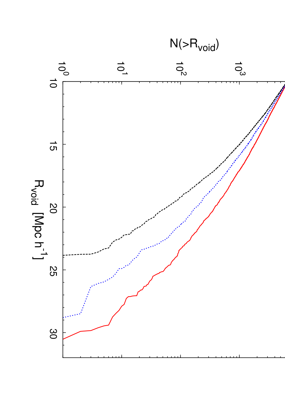
In Fig. 10 we show the cumulative number of voids with radius larger than the center of which is in the original box. One can clearly see that for a given void radius there exist more voids in the CDM than in th CDM-vde and VDE models. The void distribution reflects the behaviour of the mass function shown in Fig. 8. At redshift there exist less haloes with in the CDM model than in the other two models. Thus on average larger voids are expected.
4.5 Growth Index

The growth of the perturbations can be related to the evolution of the matter density parameter by the general relation
| (21) |
In the standard CDM cosmology, the exponent can be approximated by a constant value , although a more detailed calculation shows that this number is actually redshift dependend (Bueno Belloso et al., 2011, see ). In Fig. 11 we show the evolution of this growth index computed from our VDE-0.5, CDM-vde and CDM-0.5 simulations. As expected, we do observe that in VDE structure formation is generally suppressed with respect to CDM as an effect of the faster expansion rate. This statement is true until , when the ratio starts decreasing causing the steep increase in the growth index, eventually reducing again as soon as vector dark energy enters into the phantom regime (see Section 2), undergoing an accelerated expansion that strongly suppresses structure formation. This latter change, which takes place at , is reflected by the peak of , which is reached for the same . Actually, as stressed by different parametrizations (Bueno Belloso et al., 2011), the growth index is extremely sensitive to the value of the equation of state , although an explicit form in terms of VDE cosmology still has to be found. Indeed, the extremely different behaviour of this parameter at different redshifts is an interesting feature that clearly distinguishes the two models in a unique way: In fact, parameter-induced modification accounts for a change for the value of the growth factor, as the comparison among CDM and CDM-vde suggests. In this case we observe a slight increase of the value of at all redshifts, due to the increased growth rate in CDM-vde also shown in Fig. 5. However, these changes have no impact on the shape of this function, which keeps its mild dependence on unaltered. Therefore can be effectively used as a tool for model selection, embodying effectively VDE’s peculiar equation of state and expansion history. Current observational bounds on constrain only weakly its value at high ’s (Nesseris & Perivolaropoulos, 2008, see e.g. ) or even favour a higher (Basilakos, 2012) in contrast to theoretical calculations based on CDM. In any case, it will surely be something to be looked at in the near future, when deep surveys like Euclid (Laureijs et al., 2011) will provide stringent constraints on this quantity (Bueno Belloso et al., 2011).
5 Dark Matter Haloes
In this section we will discuss properties of (individual) haloes in VDE and CDM. In particular, we will compare the distributions of masses, shape parameter, spin parameter, concentrations and formation redshifts as well as the shape of dark matter density profiles. In this way, we will determine the most important features that characterize on the average a single cosmological model. But in addition we are also cross correlating haloes in the two models studying differences on a one-to-one basis. By this we will be able to determine how the properties of a single given structure change when switching from one cosmological picture to the other.
5.1 General properties
To have a reliable description of the general halo properties we need to properly select our sample from the catalogues, in order to include only those objects composed of a number of particle sufficient to resolve its internal structure without exceeding statistical uncertainty. Following Muñoz-Cuartas et al. (2011) and Prada et al. (2011) we set this number to approximately 500, even though other authors (see for example Macciò et al. (2007) and Bett et al. (2007)) suggest that lower values can be used, too. However, since we are dealing with different simulations run with particles of different mass, the application of this criterion is not straightforward. In fact, since our aim is to compare equivalent structures (i.e. structures with the same ) and not structures composed by an identical number of particles we need to choose our sample imposing a mass threshold . For the simulations in the box, we have chosen , which corresponds to haloes formed by at least 500 particles in VDE and CDM-vde and 715 particles in CDM; while for the larger runs we imposed a limit, i.e. 380 VDE and CDM-vde particles and 545 CDM ones. In the latter set of simulations, we see that we are including also haloes with a less than 500 particles in the VDE and CDM-vde cases; this has been done since in the trade off between resolution and sample size we have felt more comfortable using a larger number of haloes at the expense of a slight reduction in accuracy, which will be nonetheless taken into account when analyzing the results. The total number of haloes that comply with these conditions in every simulations, as well as the number of haloes that satisfy the relaxation criterion which will be discussed in Section 5.1.3, are shown in Table 2. The state of virialisation of haloes will only be taken into account below when investigating the density profiles; for the study of the (distributions of the) two-point correlation functions, the spin, and even the shape of haloes we prefer to include even un-relaxed objects as they should clearly stick out in the distributions (if present in large quantities).
| Simulation | total | relaxed | ||
|---|---|---|---|---|
| CDM-0.5 | 715 | 1704 | 1370 | |
| CDM-vde-0.5 | 500 | 5898 | 5220 | |
| VDE-0.5 | 500 | 6274 | 5569 | |
| CDM-1 | 545 | 4045 | 3533 | |
| CDM-vde-1 | 380 | 9072 | 8117 | |
| VDE-1 | 380 | 12174 | 11508 |
5.1.1 Correlation function
To study the clustering properties of the haloes in VDE cosmology, we computed the two point correlation function using the definition:
| (22) |
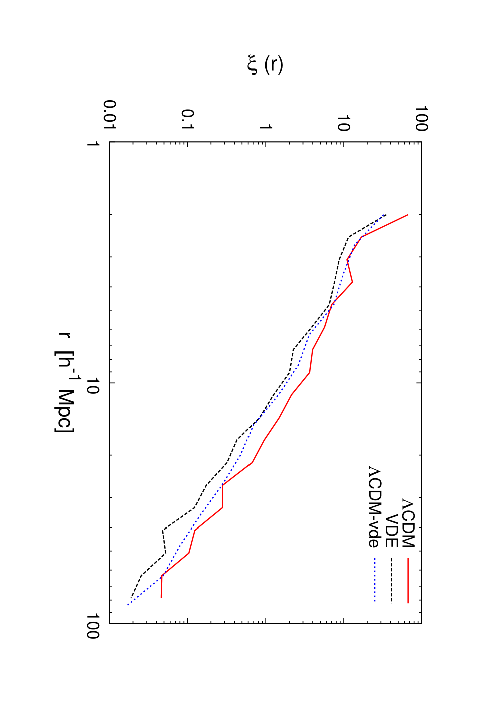
where is the total number of objects above the given mass threshold in the simulation volume , and is the total number of objects within a shell of volume and thickness (of constant logarithmic spacing in ) centered at the th object. In this case, we have limited our analysis to the 500 boxes, ignoring the 1Gpc due to their lack of small scale resolution. The results are plotted in Fig. 12, where we can see that the is slightly smaller at all scales in VDE. Although in principle we would expect VDE cosmology to have an enhanced clustering pattern due to the increased distribution of massive objects observed in the mass function, the dependence of the two point correlation function drags the total value down, making the final distribution function smaller than in CDM. In fact, a similar behaviour can be observed for CDM-vde; with a two point correlation function below CDM at practically all scales. In Table 3 we show the results of fitting to a power law from which we see that VDE is characterized by a smaller correlation length and a steeper slope .
5.1.2 Spin parameter, shape and triaxiality
Rotational properties of the haloes can be studied using the so called spin parameter , a dimensionless number that measures the degree of rotational support of the halo. Following Bullock et al. (2001), we define it as
| (23) |
where the quantities (the total angular momentum), (total mass), (circular velocity) and (radius) are all taken at the point where the average halo density becomes 200 times the critical density. Different authors have found (Barnes & Efstathiou, 1987; Warren et al., 1992; Cole & Lacey, 1996; Gardner, 2001; Bullock et al., 2001; Macciò et al., 2007; Macciò et al., 2008; Muñoz-Cuartas et al., 2011, e.g.) that the distribution of this parameter is of lognormal type
| (24) |
even though there are recent claims that this distribution has to be slightly modified (Bett et al., 2007).
Fitting the above function to our numerical sample by a non-linear Levenberg-Marquardt
least square fit we find a remarkably good agreement, shown in Fig. 13 for the combined set of haloes
of the 500 and 1Gpc simulations.
It is clear that the three models present
no substantial difference in the values of these distributions, meaning that the change of cosmology
has no impact on the rotational support of the dark matter structures.
The shape of three dimensional haloes can be modelled as an ellipsoidal distribution of particles (Jing & Suto, 2002; Allgood et al., 2006), characterized by the three axis computed by AHF as the eigenvalues of the inertia tensor
| (25) |
which is in turn obtained summing over all the coordinates of the particles belonging to the halo.
We define the shape parameter and the triaxiality parameter as
| (26) |
and we calculate the probability distributions and of the above parameters for all the objects above the aforementioned mass thresholds in our cosmological simulations, to see whether the VDE picture of structure formation induces changes in the average shape and triaxiality. Similarly to the previous case, we found again that halo shapes and triaxialities remain practically unaltered by VDE cosmolgy. This result could be expected, keeping in mind that VDE only affect background evolution: Once that structures start to form, detaching from the background evolution, they become affected by gravitational attraction only. Therefore, the internal structure of dark matter haloes remains generally unaltered by the presence of an uninteracting form of dark energy and cannot be used to discriminate between alternative cosmological paradigms. We have also verified that these results hold also when taking into account different halo samples separately, i.e. the massive ones of the 1Gpc simulations and the smaller belonging to the 500 boxes.
5.1.3 Unrelaxed haloes
Before moving to the discussion of the properties of internal structure of the haloes, and in particular the density profile, we need to introduce and motivate a second criterion of selection for our halo sample, related to the degree of relaxation of the halo. An additional check is necessary since only a fraction of the structures identified in our catalogues completely satisfies the virial condition. In unvirialized structures, infalling matter and merger phenomena may occour, heavily affecting the halo shape and thus making the determination of radial density profiles and concentrations unreliable. In fact, unrelaxed haloes are most likely to differ from an idealized spherical or ellipsoidal shape since they have a highly asymmetric matter distribution, which in turn makes the determination of the halo center an ill-defined problem, as discussed by Macciò et al. (2007) and Muñoz-Cuartas et al. (2011). Our halo finder AHF does not directly discriminate between virialized and unvirialized structures giving catalogues containing both types of objects; however, it provides kinetic and potential energy for every halo identified, thus making the computation of the viral ratio straightforward. Following one of the criteria used by Prada et al. (2011), we will consider as relaxed all the haloes satisfying the condition
| (27) |
without introducing additional parameters. Alternative ways of identifying unrelaxed structures can be found throughout the literature (Macciò et al., 2007; Bett et al., 2007; Neto et al., 2007; Knebe & Power, 2008; Prada et al., 2011; Muñoz-Cuartas et al., 2011; Power et al., 2011, e.g.); but since the results they give are qualitatively similar for reasons of computational speed and simplicity we will not make use of them. The total number of haloes satisfying the relaxation condition is shown for every cosmology in Table 2.
5.1.4 Density profiles
-body simulations have shown that dark matter haloes can be described by a Navarro Frenk White (NFW) profile (Navarro et al., 1996), which is given by
| (28) |
where the , the so called scale radius, and the are in principle two free parameters that depend on the particular halo structure. But can be written as a function of the critical density as , where
and is the concentration of the halo relating the virial radius ( in our case) to the scale radius , which will be discussed in detail in the following subsection. This description is generally valid for CDM, but simulations of ever increased resolution have actually revealed that the very central regions are not following the slope advocated by the NFW formula but rather follow a Sersic or Einasto profile (Navarro et al., 2004; Stadel et al., 2009, cf. ).
Here we want to check to which degree the modified cosmological background affects the distribution of matter inside dark matter haloes, i.e. its density profile. All our (relaxed) objects in all simulations have been fitted to the Eq. (28), and to estimate the goodness of this fit we compute for each halo its corresponding , defined in the usual way
| (29) |
where the ’s are the numerical and theoretical overdensities in units of the critical density at the -th radial bin and is the numerical Poissonian error on the numerical estimate. Since different halo profiles will be in general described by a different number of radial bins44 4 Note that our halo finder AHF uses logarithmically spaced radial bins whose number depends on the halo mass, i.e. more massive haloes will be covered with more bins., to make our comparison between different simulations and haloes consistent we need to use the reduced
| (30) |
where is the total number of points used (i.e. total number of radial bins) and is the number of degrees of freedom (free parameters).
The comparison of the distributions of the reduced values for CDM-vde, CDM and VDE haloes belonging to the two set of 500 and 1Gpc simulations, shown in Fig. 14, allows us to determine again that no substantial difference is induced by the VDE picture, for the same reasons discussed in the case of spin, shape and triaxiality distributions. The standard description of dark matter structures is thus not affected by the presence of a VDE.
5.1.5 Halo concentrations
In the last step of the analysis of the general properties of haloes we will turn to concentrations, which characterize the halo inner density compared to the outer part. This parameter is usually defined as
| (31) |
where is the previously introduced scale radius, obtained through the best fit procedure of the density distribution to a NFW profile. We would like to remind that concentrations are correlated to the formation time of the halo, since structures that collapsed earlier tend to have a more compact center due to the fact that it has more time to accrete matter from the outer parts. Dynamical dark energy cosmologies generically imply larger values as a consequence of earlier structure formation, as found in works like those by Dolag et al. (2004), Bartelmann et al. (2006) and Grossi & Springel (2009). In fact, since the presence of early dark energy usually suppresses structure growth, in order to reproduce current observations we need to trigger an earlier start of the formation process, which on average yields a higher value for the halo concentrations. However, this result does not hold in the case of coupled dark energy, where the increased clustering strength induced by a fifth force sets a later start of structure formation, as discussed in Baldi et al. (2010).
In the hierarchical picture of structure formation, concentrations are usually inversely correlated to the halo mass as more massive objects form later; -body simulations (Dolag et al., 2004; Prada et al., 2011; Muñoz-Cuartas et al., 2011) and observations (Comerford & Natarajan, 2007; Okabe et al., 2010; Sereno & Zitrin, 2011) have in fact shown that the relation between the two quantities can be written as a power law of the form
| (32) |
where and can have explicit parametrizations as functions of redshift and cosmology (Neto et al., 2007; Prada et al., 2011; Muñoz-Cuartas et al., 2011, see e.g.). We can use our selected halo samples at from the 500 and 1 Gpc simulations to obtain the and values for the CDM, CDM-vde and VDE cosmologies; the results of the best fit procedure to Eq. (32) are shown in Table 3.
These values are in good agreement with the ones found by, for instance, Dolag et al. (2004), Macciò et al. (2008) and Muñoz-Cuartas et al. (2011) (who quote for CDM values of and ); the discrepancy observed with their results is due to the fact that our results are obtained over a smaller mass range, – , whereas the previously cited works study it over an interval larger by more than three orders of magnitude, –. Still, according to our results, the relation for both the VDE and CDM-vde case is characterized by a shallower exponent and a larger . Although the magnitude of these changes is different in the two models, we can safely conclude that also in this case the results are mainly parameter-driven, i.e. due to the larger value of . Furthermore, the large error bars for scales, due to the low statistics of massive haloes complying the relaxation requirements, makes it difficult to determine to which extent the differences in the best fit relations among CDM-vde and VDE could be eventually reduced in the presence of a larger sample.
| Model | ||||
|---|---|---|---|---|
| CDM | -0.115 | 2.11 | 13.4 | -1.79 |
| CDM-vde | -0.112 | 2.21 | 12.1 | -1.91 |
| VDE | -0.098 | 2.17 | 10.1 | -1.94 |
We also need to mention that in our simulations the actual halo concentrations do not precisely follow equation Eq. (32) but rather scatter around it, as can be seen in Fig. 15, where the average per mass bin is plotted against the corresponding best fit relations. This is not really surprising, since observations (Sereno & Zitrin, 2011) and -body simulations (Dolag et al., 2004) have shown that halo concentrations are lognormally distributed around their theoretical value calculated using Eq. (32). In Fig. 16 we show that this is indeed the case: the distribution of the , where is the theoretical concentration value for a halo of mass , extremely close to a lognormal one with an almost model independent dispersion .
5.2 Cross Correlation
The next step in our analysis consists of studying the properties of the (most massive) cross correlated objects found in the three models at . Whereas in the previous section our focus was on the distribution of halo properties, this time we aim at understanding how they change switching from one model to another.
The identification of ”sister haloes” among the different cosmologies can be done using the AHF tool MergerTree, which determines correlated structures by matching individual particles IDs in different simulation snapshots. For a more elaborate discussion of its mode of operation we refer the reader to Section 2.4 in Libeskind et al. (2010) where it has been described in greater detail. This time we decided to restrict our halo sample further only picking the first 1000 most massive (CDM) haloes. The criterion of halo relaxation has of course also been taken into account when dealing with profiles and concentrations.
5.2.1 Mass and spin parameter

In the two upper panels of Fig. 17 we show the ratios of the masses and spin parameter for all the cross correlated sets of simulations; in each panel we show the ratios for the 500 simulation boxes while on the right the 1Gpc ones. Both VDE and CDM-vde show average mass and spin values scattered around values larger than one when compared to CDM, whereas the cross comparison of VDE to CDM-vde shows average ratios close to unity at all mass scales. This substantial increase in the ratios is due to the earlier beginning of structure formation, triggered by the larger and , as the comparison VDE/CDM-vde shows. As we already did in Section 5.1 when looking at the halo properties in general, we conclude that also when observing the same halo evolved under different cosmologies, the main effects are determined exclusively by the set of cosmological parameters chosen, being the imprint of the cosmological background evolution substantially negligible in this case. This makes the identification of a cosmic vector through the determination of halo properties impossible, since the background dynamics, which distinguishes VDE from any other non interacting dynamical dark energy model, does not leave any observable imprint on these scales.
5.2.2 Halo concentrations and internal structure
As done in the previous section, in the determination of halo profiles and concentrations properties we discard unrelaxed haloes, but this time in a way so that our halo sample will still be composed of the first 1000 haloes satisfying condition Eq. (27). This same halo sample has been used also in the study of the , in order to be able to compare these results with the ones obtained from concentrations consistently – although in principle formation redshifts are well defined even for unrelaxed haloes. Again, our procedure consists in fitting all the selected structure to a NFW profile, from which we will be able to derive the concentration parameter and a measure for the quality of the fit ; we will then compare these results in each cross identified objects to see how a given halo structure changes when evolved under a different cosmology. Although not shown here, no particular trend in the differences among CDM, CDM-vde and VDE pictures has been be found for either NFW , shape and triaxiality; since in all the cases the ratios of these properties among cross correlated haloes are centered around unity. Not surprisingly, we also find again a generally higher average value for the concentrations in VDE and CDM-vde with respect to CDM, (see Fig. 17) a result which again can be explained by the larger value of and . Similar concentrations for VDE and CDM-vde haloes, shown in the upper right panel of Fig. 17 can be also understood as a consequences of the similar masses of the haloes examined and the similar relations found for the two cosmologies. However, even if from CDM-vde cosmology we conclude that the different choice of , can explain in this case higher halo concentration, we need to remind that such a results is also a general feature of the dynamical nature of the dark energy fluid, as already found by Dolag et al. (2004), Bartelmann et al. (2006) and Grossi & Springel (2009).
6 Conclusions
In this work we presented an in-depth analysis of the results of a series of -body dark matter only simulations of the Vector Dark Energy cosmology proposed by Beltrán Jiménez & Maroto (2008). The main emphasis has been on the comparison to the standard CDM paradigm, using a mirror simulation with identical number of particles, random seed for the initial conditions, box size and starting redshift. An additional series of simulations for a CDM-vde cosmology have also been run using the VDE values for and within a standard CDM picture, to disentangle the effects of the parameter induced modifications to the dynamical ones coming directly from the VDE model.
The use of a modified version of the GADGET-2 code required us to check the results with particular care. A consistency check of our simulations was performed by comparing the numerical results for the evolution of the growth factor to the analytical calculations, finding an excellent agreement between the two. We further had to adapt the halo finding procedure, due to the fact that the critical density as a function of redshift , entering the definition of the halo edges, takes different values in VDE. Once halo catalogues had been obtained, we carried our analysis at two different levels, namely:
- •
we studied the very large scale clustering pattern through the computation of matter power spectra, mass, void, and two-point correlation functions;
- •
we analyzed halo structure, comparing statistical distributions and averages of spin parameters, concentrations, masses and shapes.
In the first point, making use of the full set of simulations, our analysis covered the whole masse range – as well as different redshifts, so that we could make specific VDE model predictions for the number density evolution and growth index . A distinctive behaviour, very far from the standard CDM results, has been found for , and, in particular, for the mass function that in VDE cosmology can be up to 10 times larger than the standard CDM one. The latter result is due to the earlier onset of structure formation and we have mentioned how it can be used to address current CDM observational tensions with large clusters at and possibly with early reionization epoch (Carlesi et al., 2011, cf. also).
Computing the cumulative mass function at different redshifts and making use of the CDM-vde simulations we have also observed how the condition , holding up to , induces a relative suppression of structure growth in this cosmological model, an effect that clashes with the increased matter density and . In fact, while on the one hand higher values of these parameters enhance the formation of a larger number of objects, on the other hand, background dynamics suppresses clustering and growth. The interplay and relative size of these effects has been studied using the CDM-vde simulations, showing that, for example, faster expansion in the past determines for VDE an expectation of clusters with up to times smaller than what a simple increase in and would determine. This effect has been also seen in the void distribution, where suppression of clustering prevents small structures to merge into larger one and to rather spread in the field, so that underdense regions happen to be smaller and rarer than in CDM and CDM-vde. In these latter cosmologies, in fact, a higher contrast between populated and less populated regions is observed both in the power spectrum and in the colour coded matter density.
In the second part of our work we have focused on the study of internal halo structure. We found that VDE cosmology does not induce deviations in the functional form of the dark matter halo density profiles, which are still well described by a NFW (Navarro et al., 1996) profile, nor in the distributions for the concentrations and spin parameters, which are of the lognormal type as in CDM. Shape and triaxiality are also unaffected: the distributions for the relative parameters are identical and peaked in at the same values in all the three cosmologies. The above results are a direct consequence of the fact that dark matter haloes, once detached from the general background evolution driven by the cosmic vector, evolve by means of gravitational attraction only; which is unaffected by the specific nature of dark energy. A net effect can be seen in masses, whose average values tend to be on the larger than in the CDM case by a factor of , a straightforward consequence of the larger and , as can be shown by a direct comparison of VDE to CDM-vde results, that turn out extremely close in these cases. On the other hand, the different background evolution seems to affect relations only slightly, changing the power law index and normalization by a . In this case we have also found that these values in general agree with previous results from early dark energy studies such as those by Dolag et al. (2004), even though in this case it would certainly be necessary to test the relation down to smaller mass scales, where a better tuning of the parameter would be also possible, and with a larger statistics on the higher scales. However, in general, most of the halo-level effects which seem to characterize VDE can be simply explained in terms of the different cosmological parameters, as we did comparing these results to the outcomes of CDM-vde simulations. For the first time then, through the results of the series of -body simulations, we have shown that VDE cosmology provides a viable environment for structure formation, also alleviating some observational tensions emerging with CDM. We have seen how the peculiar dynamics of this model leaves its imprint on structure formation and growth, and in particular, how it affects predictions for large scale clustering and halo properties. However, a close comparison of the deep non-linear regime results with different sets of observational data still needs to be performed, challenging us to improve the accuracy of our simulations and at the same time devise new and reliable tests which may shed some light not only on VDE but on the nature of dark energy in general.
Acknowledgements
We would like to thank Juan García-Bellido for his interesting suggestions and discussions. EC is supported by the MareNostrum project funded by the Spanish Ministerio de Ciencia e Innovacion (MICINN) under grant no. AYA2009-13875-C03-02 and MultiDark Consolider project under grant CSD2009-00064. EC also acknowledges partial support from the European Union FP7 ITN INVISIBLES (Marie Curie Actions, PITN- GA-2011- 289442). AK acknowledges support by the MICINN’s Ramon y Cajal programme as well as the grants AYA 2009-13875-C03-02, AYA2009-12792-C03-03, CSD2009-00064, and CAM S2009/ESP-1496. G. Yepes would like to thank the MICINN for financial support under grants AYA 2009-13875-C03, FPA 2009-08958, and the SyeC Consolider project CSD2007-00050. JBJ is supported by the Ministerio de Educación under the postdoctoral contract EX2009-0305 and also wishes to acknowledge support from the Norwegian Research Council under the YGGDRASIL programme 2009-2010 and the NILS mobility project grant UCM-EEA-ABEL-03-2010. We also acknowledge support from MICINN (Spain) project numbers FIS 2008-01323, FPA 2008-00592, CAM/UCM 910309 and FIS2011-23000. The simulations used in this work were performed in the Marenostrum supercomputer at Barcelona Supercomputing Center (BSC).
References
- Abazajian et al. (2009) Abazajian K. N., et al., 2009, ApJS, 182, 543
- Alimi et al. (2010) Alimi J.-M., Füzfa A., Boucher V., Rasera Y., Courtin J., Corasaniti P.-S., 2010, MNRAS, 401, 775
- Allgood et al. (2006) Allgood B., Flores R. A., Primack J. R., Kravtsov A. V., Wechsler R. H., Faltenbacher A., Bullock J. S., 2006, MNRAS, 367, 1781
- Baldi (2011) Baldi M., 2011, ArXiv e-prints
- Baldi & Pettorino (2011) Baldi M., Pettorino V., 2011, MNRAS, 412, L1
- Baldi et al. (2010) Baldi M., Pettorino V., Robbers G., Springel V., 2010, MNRAS, 403, 1684
- Barnes & Efstathiou (1987) Barnes J., Efstathiou G., 1987, ApJ, 319, 575
- Bartelmann et al. (2006) Bartelmann M., Doran M., Wetterich C., 2006, A&A, 454, 27
- Basilakos (2012) Basilakos S., 2012, ArXiv e-prints
- Beltrán Jiménez et al. (2009) Beltrán Jiménez J., Lazkoz R., Maroto A. L., 2009, Phys. Rev. D, 80, 023004
- Beltrán Jiménez & Maroto (2008) Beltrán Jiménez J., Maroto A. L., 2008, Phys. Rev. D, 78, 063005
- Bett et al. (2007) Bett P., Eke V., Frenk C. S., Jenkins A., Helly J., Navarro J., 2007, MNRAS, 376, 215
- Beutler et al. (2011) Beutler F., Blake C., Colless M., Jones D. H., Staveley-Smith L., Campbell L., Parker Q., Saunders W., Watson F., 2011, MNRAS, 416, 3017
- Brodwin et al. (2010) Brodwin M., et al., 2010, ApJ, 721, 90
- Bueno Belloso et al. (2011) Bueno Belloso A., García-Bellido J., Sapone D., 2011, JCAP, 10, 10
- Bullock et al. (2001) Bullock J. S., Dekel A., Kolatt T. S., Kravtsov A. V., Klypin A. A., Porciani C., Primack J. R., 2001, ApJ, 555, 240
- Burenin & Vikhlinin (2012) Burenin R. A., Vikhlinin A. A., 2012, ArXiv e-prints
- Carlesi et al. (2011) Carlesi E., Knebe A., Yepes G., Gottlöber S., Jiménez J. B., Maroto A. L., 2011, MNRAS, 418, 2715
- Colberg et al. (2008) Colberg J. M., et al., 2008, MNRAS, 387, 933
- Cole & Lacey (1996) Cole S., Lacey C., 1996, MNRAS, 281, 716
- Comerford & Natarajan (2007) Comerford J. M., Natarajan P., 2007, MNRAS, 379, 190
- Dolag et al. (2004) Dolag K., Bartelmann M., Moscardini L., Perrotta F., Baccigalupi C., Meneghetti M., Tormen G., 2004, Modern Physics Letters A, 19, 1079
- Enqvist et al. (2011) Enqvist K., Hotchkiss S., Taanila O., 2011, JCAP, 4, 17
- Foley et al. (2011) Foley R., et al., 2011, ApJ, 731, 86
- Gardner (2001) Gardner J. P., 2001, ApJ, 557, 616
- Gill et al. (2004) Gill S. P. D., Knebe A., Gibson B. K., 2004, MNRAS, 351, 399
- Grossi & Springel (2009) Grossi M., Springel V., 2009, MNRAS, 394, 1559
- Guy et al. (2010) Guy J., et al., 2010, A&A, 523, A7+
- Hoyle et al. (2011) Hoyle B., Jimenez R., Verde L., 2011, Phys. Rev. D, 83, 103502
- Huterer (2010) Huterer D., 2010, General Relativity and Gravitation, 42, 2177
- Jee et al. (2009) Jee M., et al., 2009, ApJ, 704, 672
- Jimenez & Maroto (2009) Jimenez J. B., Maroto A. L., 2009, AIP Conf. Proc., 1122, 107
- Jing & Suto (2002) Jing Y. P., Suto Y., 2002, ApJ, 574, 538
- Knebe et al. (2011) Knebe A., Knollmann S. R., Muldrew S. I., Pearce F. R., et al. 2011, MNRAS, 415, 2293
- Knebe & Power (2008) Knebe A., Power C., 2008, ApJ, 678, 621
- Knollmann & Knebe (2009) Knollmann S. R., Knebe A., 2009, ApJS, 182, 608
- Larson et al. (2011) Larson D., et al., 2011, ApJS, 192, 16
- Laureijs et al. (2011) Laureijs R., Amiaux J., Arduini S., Auguères J. ., Brinchmann J., Cole R., Cropper M., Dabin C., Duvet L., Ealet A., et al. 2011, ArXiv e-prints
- Lewis et al. (2000) Lewis A., Challinor A., Lasenby A., 2000, Astrophys. J., 538, 473
- Li & Barrow (2011) Li B., Barrow J. D., 2011, MNRAS, 413, 262
- Li et al. (2011) Li B., Mota D. F., Barrow J. D., 2011, ApJ, 728, 109
- Libeskind et al. (2010) Libeskind N. I., Yepes G., Knebe A., Gottlöber S., Hoffman Y., Knollmann S. R., 2010, MNRAS, 401, 1889
- Macciò et al. (2008) Macciò A. V., Dutton A. A., van den Bosch F. C., 2008, MNRAS, 391, 1940
- Macciò et al. (2007) Macciò A. V., Dutton A. A., van den Bosch F. C., Moore B., Potter D., Stadel J., 2007, MNRAS, 378, 55
- Muñoz-Cuartas et al. (2011) Muñoz-Cuartas J. C., Macciò A. V., Gottlöber S., Dutton A. A., 2011, MNRAS, 411, 584
- Navarro et al. (1996) Navarro J. F., Frenk C. S., White S. D. M., 1996, ApJ, 462, 563
- Navarro et al. (2004) Navarro J. F., Hayashi E., Power C., Jenkins A. R., Frenk C. S., White S. D. M., Springel V., Stadel J., Quinn T. R., 2004, MNRAS, 349, 1039
- Nesseris & Perivolaropoulos (2008) Nesseris S., Perivolaropoulos L., 2008, Phys. Rev. D, 77, 023504
- Neto et al. (2007) Neto A. F., et al., 2007, MNRAS, 381, 1450
- Okabe et al. (2010) Okabe N., Takada M., Umetsu K., Futamase T., Smith G. P., 2010, PASJ, 62, 811
- Perlmutter et al. (1999) Perlmutter S., et al., 1999, ApJ, 517, 565
- Power et al. (2011) Power C., Knebe A., Knollmann S. R., 2011, ArXiv e-prints
- Prada et al. (2011) Prada F., Klypin A. A., Cuesta A. J., Betancort-Rijo J. E., Primack J., 2011, ArXiv e-prints
- Raičević et al. (2011) Raičević M., Theuns T., Lacey C., 2011, MNRAS, 410, 775
- Riess et al. (1998) Riess A. G., et al., 1998, AJ, 116, 1009
- Sereno & Zitrin (2011) Sereno M., Zitrin A., 2011, ArXiv e-prints
- Sherwin et al. (2011) Sherwin B. D., et al., 2011, Physical Review Letters, 107, 021302
- Springel (2005) Springel V., 2005, MNRAS, 364, 1105
- Stadel et al. (2009) Stadel J., Potter D., Moore B., Diemand J., Madau P., Zemp M., Kuhlen M., Quilis V., 2009, MNRAS, 398, L21
- Vikhlinin et al. (2009) Vikhlinin A., et al., 2009, ApJ, 692, 1060
- Warren et al. (1992) Warren M. S., Quinn P. J., Salmon J. K., Zurek W. H., 1992, ApJ, 399, 405
- Wen et al. (2010) Wen Z. L., Han J. L., Liu F. S., 2010, MNRAS, 407, 533
- Zel’Dovich (1970) Zel’Dovich Y. B., 1970, A&A, 5, 84