University of California, Berkeley, CA 94720 \secondemailkirby@math.berkeley.edu \primaryclass57M50 \secondaryclass57R45, 57R65
Trisecting –manifolds
Abstract
We show that any smooth, closed, oriented, connected –manifold can be trisected into three copies of , intersecting pairwise in –dimensional handlebodies, with triple intersection a closed –dimensional surface. Such a trisection is unique up to a natural stabilization operation. This is analogous to the existence, and uniqueness up to stabilization, of Heegaard splittings of –manifolds. A trisection of a –manifold arises from a Morse –function and the obvious trisection of , in much the same way that a Heegaard splitting of a –manifold arises from a Morse function and the obvious bisection of .
keywords
Morse 2-function, 4-manifold, Heegaard splitting, Heegaard triple1 Introduction
Consider first the –dimensional case of an oriented, connected, closed –manifold . From a Morse function with only one critical point of index zero and one of index three, and all critical points of index mapping to , we see that and are solid handlebodies, .
For uniqueness, we use Cerf theory [3] to get a homotopy between and (each giving Heegaard splittings) where this homotopy introduces no new critical points of index zero or three. There are births and deaths of canceling pairs of index one and two critical points, but these stabilize the Heegaard splittings by connected summing with the standard genus one splitting of . The homotopy can be chosen to keep the index one critical values below and the index two above. Then handle slides between –handles, or –handles, take one Heegaard splitting to the other. (This is a now well known Cerf theoretic proof of the Reidemeister-Singer theorem [9][11] which was originally proved combinatorially e.g. [10].)
Recall that a Heegaard diagram for a Heegaard splitting is a triple where is the Heegaard surface, and each of and is a –tuple of simple closed curves in which bounds a basis of compressing disks in each of the two handlebodies. Thus every –manifold is described by a Heegaard diagram, and two Heegaard diagrams describe diffeomorphic –manifolds if and only if they are related by stabilization, handle slides, and diffeomorphisms of .
We now set up an analogous story in dimension four: Let with . Given an integer , let be the standard genus Heegaard splitting of obtained by stabilizing the standard genus Heegaard splitting times.
Definition 1.
Given integers , a –trisection (see Figure 1) of a closed, connected, oriented –manifold is a decomposition of into three submanifolds satisfying the following properties:
- 1.
For each , there is a diffeomorphism .
- 2.
For each , taking indices mod , and .
Remark 2.
Note that the triple intersection is a surface of genus and that . Thus is determined by and , and for this reason we will often refer to a –trisection of simply as a genus trisection of . Also note that, for a fixed , different trisections thus have the same genera mod .
Given a –trisection , consider the handlebodies and the central genus surface . A choice of a system of compressing disks on for each of the three handlebodies gives three collections of curves: , and , such that compressing along gives , compressing along gives and compressing along gives . Furthermore, each pair , and is a Heegaard diagram for .
Definition 3.
A –trisection diagram is a –tuple such that each triple , and is a genus Heegaard diagram for . The –manifold determined in the obvious way by this trisection diagram will be denoted .
Theorem 4 (Existence).
Every closed, connected, oriented –manifold has a –trisection for some . Furthermore, and are such that has a handlebody decomposition with –handle, –handles, –handles, –handles and –handle.
2pt \pinlabel at 35 85 \pinlabel at 65 33 \pinlabel at 95 85
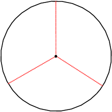
Remark 5.
There are two trivial consequences of the handle decomposition mentioned in the theorem which are worth noting:
- 1.
If , i.e. , and are each –balls, then has no – or –handles, and is thus simply-connected.
- 2.
If , then has no –handles, so .
The following is immediate:
Corollary 6.
Every closed –manifold is diffeomorphic to for some trisection diagram .
Remark 7.
Readers familiar with the Heegaard triples used [8] to define the Heegaard-Floer –manifold invariants will see that a trisection diagram is a special type of Heegaard triple and may suspect that this corollary follows fairly quickly from the Heegaard triple techniques in [8]. In all fairness this is probably true; we will present two proofs of Theorem 4, one of which tells the story of how we discovered the result using Morse –functions, while the other is more in the spirit of [8], directly using ordinary handle decompositions. In some sense, then, our existence result can be thought of as a particularly nice packaging of the topological setup for [8].
Exactly as with Heegaard splittings in dimension , our uniqueness result for trisections of –manifolds is uniqueness up to a stabilization operation, which we now define. The idea is illustrated in Figure 2, in dimension .
2pt
\pinlabel at 82 227
\pinlabel at 223 90
\pinlabel at 251 183
\pinlabel at 210 223
\pinlabel at 78 161
\pinlabel at 243 125
\endlabellist
Definition 8 (Stabilization).
Given a –manifold with a trisection , we construct a new trisection , as follows: For each , let be the handlebody , with boundary . Let be a properly embedded boundary parallel arc in each , such that the end points of , and are disjoint in . Let be a closed –dimensional regular neighborhood of in (thus diffeomorphic to ), with , and disjoint. Then we define:
- •
- •
- •
The operation of replacing with is called stabilization.
Since any two boundary parallel arcs in a handlebody are isotopic, it is clear that this operation does not depend on the choice of arcs or neighborhoods.
In terms of trisection diagrams we have:
Definition 9.
Given a trisection diagram , the trisection diagram obtained by connected summing with the diagram in Figure 3 is called the stabilization of .
2pt
\endlabellist
We prove the following fact at the beginning of Section 5:
Lemma 10.
If is a trisection of , with genus and diagram , and is a stabilization of , then is also a trisection of , with genus and diagram , the stabilization of .
The reader may find Figure 2 useful in proving this lemma before reading our proof.
Theorem 11 (Uniqueness).
Given two trisections of , and , then after stabilizing each trisection some number of times, there is a diffeomorphism isotopic to the identity with the property that for each . In particular, for in , and .
Corollary 12.
Given trisection diagrams and , the corresponding –manifolds and are diffeomorphic if and only if and are related by stabilization, handle slides, and diffeomorphism. “Handle slides” are slides of ’s over ’s, ’s over ’s and ’s over ’s.
Proof.
Any two handle decompositions of a fixed genus handlebody, each with one –handle and –handles, are related by handle slides; this is proved in [5]. ∎
2 Discussion and examples
We begin with a few explicit examples of trisections and corresponding trisection diagrams.
- •
can be explicitly divided into three pieces , giving a genus trisection of . The diagram is with no curves.
- •
Stabilizing the genus trisection of gives a genus trisection, with trisection diagram shown in Figure 3. Since it is not known if the mapping class group of is trivial, we cannot say that the diagram determines the trisection up to isotopy, but the original description of stabilization of trisections (as opposed to stabilization of trisection diagrams) does determine this trisection up to isotopy, and thus we call this the standard genus trisection of .
- •
There is an obvious connected sum operation on trisected –manifolds, obtained by removing standardly trisected balls from each manifold and gluing along the boundary spheres so as to match the trisections. Stabilization can then also be defined as performing a connected sum with with its standard genus trisection.
- •
The standard toric picture of as a right triangle gives a natural trisection into three pieces as the inverse images under the moment map of the three pieces of the right triangle shown in Figure 4. These pieces are diffeomorphic to but they intersect along solid tori all meeting along a central fiber diffeomorphic to , so that this is a genus trisection of . The trisection diagram shows a –, a – and a – curve; this is because the normals to the edges of the moment polytope tell us the direction in the torus which collapses along that edge. Alternatively, this trisection can be seen simply as the –handle, –handle and –handle in the standard handle decomposition of , and the framing on the –handle can be seen in the –curve.
\labellist\hair2pt \pinlabel at 25 55 \pinlabel at 25 25 \pinlabel at 55 25 \pinlabel [r] at 160 24 \pinlabel [br] at 204 45 \pinlabel [l] at 215 52 \endlabellist

Figure 4: Trisection of . - •
Reversing the orientation of the central surface in a trisection diagram reverses the orientation of the –manifold; i.e. . Thus has a genus trisection, with trisection diagram given by a –, – and –curve.
- •
Looking at the standard toric picture of as a square also leads to a natural trisection of as follows: We divide the square into four regions labelled , , and as indicated in Figure 5, and label the inverse images of these regions in with the same labels.
\labellist\hair2pt \pinlabel at 44 44 \pinlabel at 110 35 \pinlabel at 30 110 \pinlabel at 104 104 \endlabellist
Figure 5: Trisection of . Each of , , and is a –ball, and in fact they give the standard handle decomposition of , with being the –handle, and being the –handles and being the –handle. Note that is , with being and being . Let be a point in and let be the arc . Remove a tubular neighborhood of this arc from and and add it as a tube joining to . The union of and with this tube is the of our trisection, and the new and are the results of removing the tube from the original and . A little thought shows that this is a trisection with (each piece is a –ball) and . (Thanks to Bob Edwards for giving us the initial picture that led to this description.)
- •
It may not be entirely obvious how to draw the trisection diagram for the above trisection of . However, it is not hard to draw a genus trisection diagram from scratch that does give . In Figure 6 we show this diagram, as well as a diagram for and a diagram for . We leave it to the reader to see how to relate these diagrams to the standard handle diagrams for these –manifolds. It is also an illuminating exercise, knowing that , to verify Corollary 12 in this case. The earlier discussion of connected sums and of gives a trisection diagram for and one checks that this is equivalent to that in Figure 6 for via handle slides and diffeomorphism of . (It turns out that in this case we do not need stabilization.)
\labellist\hair2pt \pinlabel [b] at 54 49 \pinlabel [b] at 170 49 \pinlabel [b] at 272 50 \endlabellist

Figure 6: Various genus trisection diagrams.
Now we briefly discuss trisection diagrams more generally. Given a trisection diagram , the –manifold is constructed by attaching –dimensional –handles to along , and , with framings coming from , and the remainder of is – and –handles. Recall that there is a unique way, up to diffeomorphism, to attach the – and –handles [7].
Since each of , and is a Heegaard diagram for , each can, after a sequence of handle slides, be made to look like the standard genus Heegaard diagram of . However, there is no reason to expect that we can simultaneously arrange for all three pairs of sets of curves to be standard.
Figure 7 illustrates a general trisection diagram (except that only one curve is shown) where we have made the standard, where is red and is blue; the reds and blues give the standard genus Heegaard diagram for . The important point is that most of the information about the –manifold is then carried by the curves (one of which is drawn here in green). These green curves can be drawn anywhere with the proviso that some sequence of handle slides of the greens amongst the greens and the reds amongst reds, followed by a diffeomorphism of , can make the reds and greens look like the reds and blues. The same proviso holds for the greens and blues, but a different sequence of handle slides and a different diffeomorphism may be required.
2pt \pinlabel [t] at 126 8 \pinlabel [t] at 332 10 \pinlabel [r] at 45 44 \pinlabel [l] at 49 42 \pinlabel [b] at 51 96 \pinlabel [l] at 277 44 \pinlabel [r] at 267 68 \endlabellist
In fact, if a trisection diagram is drawn so that ’s and ’s are standard as in Figure 7, then a framed link diagram for is obtained by erasing the last ’s and ’s (which appear as meridian–longitude pairs) and then replacing each of the first parallel pairs of ’s and ’s by a parallel dotted circle (–handle) pushed slightly out of . The ’s remain as the attaching maps for –handles, and their framings come from the surface .
An extended example: –manifold bundles over . (Thanks to Stefano Vidussi for asking interesting questions that led to this example.) Suppose fibers over , , with fiber a closed, connected, oriented –manifold , and monodromy .
A trisection of is not immediately obvious, just as a bisection (Heegaard splitting) is not immediate when a –manifold fibers over a circle: .
In the latter case, one takes two fibers over distinct points of , separating into two copies of . Choose a Morse function on with one critical point of index and thus one –handle . Remove from one and add it to the other copy of . This turns the first copy into a handle body with –handles, and adds a –handle to the second copy. Again let be the –handle of the second copy (disjoint from the first ), and remove from the second copy of and add it to the first copy. Now both copies are handle bodies with –handles and we have the desired Heegaard spitting.
In the –dimensional case, , pick a Morse function with only one critical point of index and only one of index ( could give a minimal genus Heegaard splitting if desired).
Then is another Morse function on with the same kind of critical points, and can be isotoped so as to fix the maximum and the minimum . Then there is a homotopy , such that
- 1.
,
- 2.
on and and there are no other definite critical points of ,
- 3.
is a Morse function for all but a finite number of values of at which has a birth or a death of a cancelling pair of indefinite critical points.
Since , property (1) allows us to define
by setting . To check, note that .
Thus we have a smoothly varying family of Morse functions on the fibers of , except for the births and deaths. There are an equal number of births and deaths because and have the same number of critical points. Then we can make all the births happen earlier at and the deaths later at , and furthermore by an isotopy of , the births and deaths can be paired off and happen at the same points of . In that case the pairs can be merged and then is a family of Morse functions of the fibers of with only one fixed maximum and minimum and critical points of indices and . Furthermore, it is straightforward to arrange that all critical points of index (resp ) take values in a small neighborhood of (resp. ) for each .
Now draw a hexagonal-like grid on as in Figure 8 and label the boxes with . Recall that the left and right ends are identified so as to have .
2pt \pinlabel at 19 31 \pinlabel at 64 31 \pinlabel at 123 31 \pinlabel at 168 31 \pinlabel at 34 65 \pinlabel at 94 65 \pinlabel at 153 65 \pinlabel [tr] at 6 4 \pinlabel [r] at 4 32 \pinlabel [r] at 4 64 \pinlabel [r] at 4 92 \pinlabel [t] at 183 3 \pinlabel [l] at 183 92 \pinlabel [bl] at 64 55 \pinlabel [t] at 82 2 \pinlabel [l] at 100 42

The trisection of into is to be made by tube-connect summing the pre images under of the ’s in Figure 8. Over each vertical line segment in Figure 8 is which is defined to be a –dimensional handle body with –handles, so over the interior vertices lie surfaces . Over the diagonally sloped line segments lie –manifolds .
Let be the –handle in and define a –dimensional –handle to be a thickening of into the bounding ’s on either side of . Add such a –handle to connect each to another across a sloping line segment, for . Doing this twice for , once along a SW-NE sloping line and once along a NW-SE sloping one as in Figure 9, we see that has become connected and is a –dimensional handlebody with –handles. Similarly with and .
2pt \pinlabel [r] at 2 24 \pinlabel at 64 31 \pinlabel at 123 31 \pinlabel at 34 65 \pinlabel at 94 65 \pinlabel at 153 65 \pinlabel–h [tl] at 48 48 \pinlabel–h [bl] at 138 48

Next we calculate . Its various parts are shown in Figure 10. Note that the sloping edges with labels arise from by having removed the . Thus we have –handles, and three of the –handles cancel –handles leaving . Then the central fiber of the trisection has genus and gives a Heegaard splitting of . Note that and we can check that .
2pt \pinlabel at 19 28 \pinlabel at 64 28 \pinlabel at 123 28 \pinlabel at 168 28 \pinlabel at 34 68 \pinlabel at 94 68 \pinlabel at 153 68 \pinlabel–h [bl] at 20 48 \pinlabel–h [tl] at 48 48 \pinlabel–h [tl] at 110 48 \pinlabel–h [bl] at 138 48 \pinlabel [l] at 36 20 \pinlabel [l] at 125 75 \pinlabel [bl] at 79 48 \pinlabel [tl] at 168 48

Surface bundles over . Now suppose that fibers over with fiber a closed surface of genus . We construct a trisection in a similar fashion to the preceding example.
Let be the fibration. Identify with a cube and trisect as , where each is the union of two opposite (closed) faces of the cube. Choose disjoint sections , and over , and , respectively, and let be a closed tubular neighborhood of , for , with the ’s also disjoint. The trisection of is where
with indices taken mod .
We now verify that this is indeed a trisection, and compute and along the way. First, is two copies of . Next, removing leaves us with two copies of , where has genus and one boundary component. Thus has two –handles and –handles. Finally, is two –handles connecting the two components of . Thus one of the –handles is cancelled by one of these two –handles, and we are left with one –handle and –handles.
Now we consider the pairwise intersections. The –dimensional intersection is the union of four pieces:
- •
: Since and intersect along four edges of the cube, this is four copies of , where has genus and two boundary components. In other words, this –manifold is built from four –handles and –handles.
- •
: This sits over the four edges making up , and thus contributes four –handles, two connecting two of the components above, and two connecting the other two. Cancelling two of the –handles from the preceding step with two of these –handles, we are left with two –handles and –handles.
- •
: This is just , which is two copies of , joining up the four copies of , from the first step above, in pairs, with the factor in lining up with one of the boundary components of the factor of . Thus we get two new –handles and two new –handles. One of the –handles cancels a –handle, and both –handles cancel –handles. This leaves us with one –handle and –handles.
- •
: This is empty.
Thus is a –dimensional handlebody with genus , and the same holds for and .
The triple intersection is necessarily the boundary of each pairwise intersection, so we see that we have a trisection with and . This gives , which is what we expect for a genus bundle over .
When this technique is applied to we get the genus diagram in Figure 11. With some work this can be shown to be handle slide and diffeomorphism equivalent to a single stabilization of the genus diagram of in Figure 6.
2pt
\endlabellist
Gluing maps: A –manifold with a trisection is determined up to diffeomorphism by the data of , and three gluing maps between the sectors; see Figure 12. Here we discuss this gluing data carefully and show how to reduce the data to two elements of the mapping class group of a closed genus surface satisfying certain constraints.
2pt
\pinlabel at 22 71
\pinlabel at 53 20
\pinlabel at 80 73
\pinlabel [tr] at 43 50
\pinlabel [tl] at 60 49
\pinlabel [b] at 52 65
\pinlabel [tr] at 25 40
\pinlabel [tl] at 78 38
\pinlabel [b] at 52 86
\pinlabel [r] at 41 84
\pinlabel [br] at 23 48
\pinlabel [tl] at 32 31
\pinlabel [tr] at 74 31
\pinlabel [bl] at 82 48
\pinlabel [l] at 63 85
\pinlabel at 51 55
\endlabellist
Let , and be copies of . Let be the standard genus Heegaard splitting of with the Heegaard surface, with a fixed identification . We can then construct a –manifold with three diffeomorphisms , for , such that glues to (indices taken mod. ) by gluing the copy of in to the copy of in . Let and note that we need to be isotopic to the identity in order for the resulting manifold to close at the central fiber . Furthermore, since an automorphism of a –dimensional handlebody is completely determined up to isotopy by its restriction to the boundary surface, this entire construction is actually determined by the two (isotopy classes of) maps , with .
However, this characterization is slightly misleading because an arbitrary pair of mapping classes of does not necessarily produce a trisected –manifold: We need that each of , and extends to a diffeomorphism , a slightly messy condition that is not entirely trivial to check.
Gluing maps from model manifolds: In fact we can reduce the gluing map data to a single gluing map if we construct trisected –manifolds by cutting open and regluing fixed model trisected manifolds. For each let . Note that has a standard –trisection , because has a standard –trisection and has a standard –trisection. Also, for each such , fix an identification of with the standard genus handlebody . Then any other –manifold with a –trisection is obtained from by cutting , and apart, regluing to by some automorphism of , and then observing that gluing in amounts to attaching a collection of –handles and a –handle, so that no other gluing data needs to be specified. Again, not any automorphism will work, but now one needs to verify that is diffeomorphic to in order to verify that actually produces a closed trisected –manifold.
Lagrangians, Maslov index, signature and intersection triples: Given a genus trisection diagram , one can write down a triple of integer matrices, giving the intersection pairing between curves. Our uniqueness theorem tells us that this intersection triple is uniquely determined by the diffeomorphism type of up to elementary row-column operations and stabilization. Here, the row-column operations are precisely those corresponding to handle slides. Thus, for example, sliding over corresponds to adding row to row in while simultaneously adding column to column in . Stabilization replaces with the following triple:
The fact that each pair of collections of curves gives a Heegaard diagram for tells us that each of the three matrices is, independently, row-column equivalent to . We thus have an invariant of –manifolds taking values in this set of triples, subject to this condition, modulo an interesting equivalence relation. Of course, this invariant may contain nothing more than homological information, for example, but even if that were true it would be interesting to understand exactly how this works.
Alternatively, one can define three Lagrangian subspaces in the symplectic vector space ; i.e. is the kernel of the map where is the handlebody determined by the curves, and so on. One immediately recovers the three intersection matrices above as the symplectic form on restricted to each pair of Lagrangians, relative to chosen bases on the Lagrangians. Thus our uniqueness theorem also gives us a –manifold invariant taking values in the set of quadruples , where is a symplectic vector space and the ’s are linear Lagrangian subspaces, subject again to the condition, modulo an equivalence relation. This equivalence relation is linear symplectomorphism and stabilization, which in this case means taking the direct sum with .
This Lagrangian set up has in fact been studied in the more general context of Wall’s [13] nonadditivity of the signature. A direct application of the interpretation in [2] of Wall’s nonadditivity result shows that the signature of a closed –manifold with a trisection is precisely the Maslov index of this associated triple of Lagrangians.
However, one expects more information to be encoded in these Langrangians triples than just the signature. In particular, the Maslov index ignores the integer lattice structure of . Quotienting out by this lattice gives us a triple of Lagrangian –tori in a symplectic –torus, and one again gets a –manifold invariant taking values in these triples mod symplectomorphism and stabilization. It seems that a further study of this set up could be fruitful.
Curve complex perspective: To record much more data than simply the homology classes of curves which bound disks in the three handlebodies, we can consider, for each handlebody , and , the subsets , and , respectively of the curve complex for given by those essential simple closed curves which bound disks in the respective handlebody. Because each pair of handlebodies gives , we know that the three intersections , and are nonempty. This perspective raises many interesting questions, such as: What is the minimal area of a triangle with vertices in the three intersections? If is nonempty, what does that tell us about ? If the gluing map coming from the model manifold construction described above is, for example, pseudo-Anosov, does this tell us that the three subcomplexes are “far apart” in any sense?
3 Existence via Morse –functions
The proof presented in this section is an application of tools developed in [4], using Morse –functions. In the following section we will rewrite the proof entirely in terms of ordinary Morse functions and handle decompositions, but the trisection is so natural from the point of view of Morse –functions that we feel this proof is worth presenting. However, to give the basic idea for those most comfortable with the language of handle decompositions, our construction ends up putting the – and –handles of into , the – and –handles into , and the –handles together with some “connective tissue” into .
A Morse –function is a smooth, stable map ; in this paper we will always map to . (Stable implies generic when mapping to dimension two.) Just like Morse functions, Morse –functions can be characterized by local models, and we now give these local models only in the case of , i.e. we are considering an –valued Morse –function on a –manifold :
- 1.
Each regular value has a coordinate neighborhood over which looks like for some closed fiber surface .
- 2.
The set of critical points of is a smooth –dimensional submanifold such that is an immersion with isolated semicubical cusps and crossings. The non-cusp points of are called fold points, and arcs of such points are called folds.
- 3.
Each point which is not a cusp or crossing has a neighborhood with coordinates , with diffeomorphic to for a –dimensional cobordism , so that , where is a Morse function on with one critical point. The index of this critical point is then called the index of the fold, although this is only well-defined up to . When the image of the fold is co-oriented, the index is well-defined by insisting that the –coordinate on increases in the direction of this co-orientation.
- 4.
Each cusp point has a neighborhood with coordinates , with , so that , where is a –parameter family of Morse functions on with no critical points for and a birth of a cancelling pair of critical points at . In our examples, these two critical points will always be of index and .
- 5.
Each crossing point has a neighborhood with coordinates , with , so that , where is a –parameter family of Morse functions on with two critical points for all , such that the critical values cross at . In our examples, these two critical points will never be of index or .
The basic example of a Morse –function is for an arbitrary generic homotopy between two given Morse functions , and the message of the above local models is that Morse –functions look locally like homotopies between Morse functions, but globally we may not have a preferred “time” direction. When is of the form , we call a Cerf graphic [3]. Conversely, given a Morse –function and a rectangle in which has no vertical tangencies, we can find coordinates in which is of this form , and so again we will say that is a Cerf graphic in this rectangle.
There is one move on Morse –functions (i.e. local model for a generic homotopy between Morse –functions) that is central to this paper, which we call the “introduction of an eye”. In a local chart in which a given Morse –function on a –manifold has no critical points, we can assume has the form or, equivalently, with . Introducing a parameter we get a homotopy , with corresponding to the given map and the end result of “introducing an eye”. Figure 13 shows the image of the critical locus at , justifying the terminology. Note that this is a Cerf graphic in which, as increases from to , we see a Morse function on space which starts with no critical points, develops a cancelling pair of index and critical points, and then the cancelling pair disappears again so that at there are again no critical points.
2pt \pinlabel [b] at 64 75 \pinlabel [l] at 128 38 \endlabellist
Note also that the introduction of an eye takes place in a ball and is localized to a disk in the fiber cross a disk in the base; thus, as long as fibers are connected, we need only specify a disk in the base without critical points and then there is a unique, up to isotopy, way to introduce an eye in that disk.
Proof of Existence, Theorem 4.
Throughout we will use coordinates on , with horizontal and vertical. Here is an outline of the proof:
- 1.
First we will show that there is a Morse –function such that the image of the fold locus is as in Figure 14. In this and the following figures, three dots between two curves indicate that there are some number of parallel copies of the two curves in between. Fold indices are indicated with labelled transverse arrows. Boxes with folds coming in from the left and out at the right represent arbitrary Cerf graphics, with the left-right axis being time. Note that a Cerf graphic may contain left-cusps, right-cusps and crossings, but may not contain any vertical tangencies on the image of the fold locus.
\labellist\hair2pt \pinlabel [l] at 353 17 \pinlabel [b] at 16 209 \pinlabel [t] at 40 16 \pinlabel [t] at 56 16 \pinlabel [t] at 72 16 \pinlabel [t] at 116 16 \pinlabel [t] at 140 16 \pinlabel [t] at 284 16 \pinlabel [t] at 304 16 \pinlabel [t] at 320 16 \pinlabel [tl] at 180 40 \pinlabel [tl] at 180 200 \pinlabel [tl] at 188 56 \pinlabel [tl] at 188 136 \pinlabel [tl] at 256 60 \pinlabel [tl] at 256 160 \endlabellist

Figure 14: The image of the fold locus for . - 2.
In Figure 14, the vertical tangencies of the folds are highlighted in red; these become critical points of the projection . These critical values in are also indicated at the bottom of the diagram along the –axis, with their indices.
- 3.
After constructing , we will show to homotope to such that the image of the fold locus for is as in Figure 15. Here the two Cerf graphics have no cusps. We have achieved two goals here: (1) Splitting the Cerf graphic into two, each involving only critical points of the same index and no cusps. (2) Replacing each kink that corresponds to an index critical point of with a pair of cusps.
\labellist\hair2pt \pinlabel [tl] at 180 40 \pinlabel [tl] at 188 56 \pinlabel [tl] at 188 136 \pinlabel [tl] at 180 200 \pinlabel [tl] at 236 60 \pinlabel [tl] at 236 140 \endlabellist
Figure 15: The image of the fold locus for . - 4.
Figure 16 is simply a redrawing of Figure 15 that highlights a natural trisection of into three sectors , and . Note that the critical locus over each sector consists of components, where is the genus of the central fiber. Also, each such component has at most one cusp. We no longer indicate the indices of the folds; the outermost fold is index pointing inwards, and all other folds are index pointing in.
\labellist\hair2pt \pinlabel at 24 206 \pinlabel [tr] at 100 5 \pinlabel [bl] at 234 164 \endlabellist
Figure 16: A more symmetric drawing of the image of the fold locus for . We no longer indicate the indices of the folds; the outermost fold is index going inwards, the others are index going inwards. - 5.
The form of the folds in Figure 16 is a special case of the form shown in Figure 17, where now we are not paying attention to which folds in a given sector, with or without cusps, connect to which folds in the next sector, with or without cusps, and we allow for arbitrary Cerf graphics (without cusps) between the sectors.

Figure 17: A slightly more general form for the image of the fold locus, which fits . - 6.
Now we have such that the image of the fold locus is as in Figure 17. At this point we could take and we would have each diffeomorphic to for different ’s. There is one last step to arrange that the ’s are equal: In fact, is equal to the number of folds in sector without cusps. We will show how to add a fold without a cusp to any one sector while adding a fold with a cusp to each of the other two sectors. This allows us to construct a homotopy from to , such that has the image of its fold locus of the same form as (i.e. as in Figure 17), with the same number of folds without cusps in each sector, i.e. .
- 7.
Finally we will justify the claim that each is diffeomorphic to with overlap maps as advertised.
We now fill in the details.
Begin with a handle decomposition of with one –handle, –handles, –handles, –handles and one –handle. The union of the – and –handles, is diffeomorphic to . Map this to by where is the standard Morse function with one index critical point and index critical points. Post-compose this map with a diffeomorphism from to a half-disk and we have constructed on the union of the – and –handles so that the image of the fold locus is as in the right half of Figure 18.
2pt \pinlabel [tl] at 37 33 \pinlabel [tl] at 97 52 \pinlabel [t] at 176 65 \pinlabel [t] at 197 50 \endlabellist
Now note that sits over the right edge of the half disk in Figure 18 and that the vertical Morse function on , i.e. is the standard Morse function with index critical points and index critical points, inducing the standard genus splitting of , with Heegaard surface .
Consider the framed attaching link for the –handles of . Generically will be disjoint in from the ascending –manifolds of the index critical points of as well as the descending –manifolds of the index critical points. Thus can be projected onto the Heegaard surface along gradient flow lines to give an immersed curve in with at worst double points. By adding kinks if necessary, we can assume that the handle framing of agrees with the “blackboard framing” coming from . Then by stabilizing this Heegaard splitting once for each crossing of , we can resolve these crossings and get to lie in the Heegaard surface with framing coming from the surface. This process translates into an extension of the thus-far constructed from to with fold locus as in Figure 19, with one cusp for each stabilization. In other words, the sequence of stabilizations translates into a homotopy from , the standard Morse function on , to , the stabilized Morse function. This homotopy then becomes a Morse –function on the collar .
2pt
\pinlabel [tr] at 12 65
\pinlabel [t] at 30 50
\pinlabel [tl] at 124 37
\pinlabel [tl] at 124 76
\endlabellist
Now let refer to the stabilized Heegaard surface, in which lies. Attaching a –dimensional –handle to along a component of is the same as attaching times a –dimensional –handle to along . In Figure 20 we show the resulting Morse –function at the left, where the handle sits over a vertical rectangle. Next we bend this rectangle to make the image again a half-disk. Finally, noting that the vertical Morse function at the right edge now has an index critical value below an index critical value, we switch these values to get the Morse –function at the right side of Figure 20.
2pt \pinlabel [tl] at 64 12 \pinlabel [l] at 58 27 \pinlabel [bl] at 64 149 \pinlabel [l] at 59 132 \pinlabel [tr] at 78 77 \pinlabel [tl] at 173 12 \pinlabel [l] at 167 27 \pinlabel [bl] at 173 149 \pinlabel [l] at 168 132 \pinlabel [br] at 177 62 \pinlabel [tr] at 178 98 \pinlabel [tr] at 270 12 \pinlabel [br] at 278 58 \pinlabel [br] at 270 149 \pinlabel [tr] at 278 103 \endlabellist
Note that everything in the preceding paragraph happened in a neighborhood of , so that the rest of still lies in the middle Heegaard surface for the Morse function at the right edge of the final diagram in Figure 20. Thus we can attach each –dimensional –handle this way to get the Morse –function at the left side of Figure 21. Each –handle of corresponds to a kink in the image of the folds, i.e. a smoothly immersed arc with a single transverse double point. Repeating our construction for with the union of the – and –handles, we construct the Morse –function at the right side of Figure 21. The two halves give vertical Morse functions on the boundary of the union of the – and –handles, which are related by some Cerf graphic. Putting this Cerf graphic in between the two parts of Figure 21 gives us as in Figure 14.
2pt
\pinlabel [tr] at 83 11
\pinlabel [br] at 96 66
\pinlabel [br] at 82 149
\pinlabel [tr] at 95 95
\pinlabel [tl] at 130 12
\pinlabel [r] at 139 40
\pinlabel [bl] at 130 148
\pinlabel [r] at 138 120
\endlabellist
To get to Figure 15, first we take the Cerf graphic section of Figure 14 and pull the births (left-cusps) to the left of the Cerf graphic and the deaths (right-cusps) to the right, and then pull all index critical points below all index critical points. Then the left-cusps can be pulled further left, past the kinks which correspond to –dimensional –handles, because the –dimensional –handle attachments are independent of the –dimensional stabilizations corresponding to the cusps. This is shown in Figure 22.
2pt
\pinlabel at 10 190
\pinlabel at 190 190
\pinlabel at 10 90
\pinlabel at 190 90
\endlabellist
Next we homotope the kinks into pairs of cusps as in Figure 23. The first step of Figure 23 introduces a swallowtail at the vertical tangency of the kink; this move has been discussed extensively elsewhere [6] and is a standard singularity that occurs in a homotopy between homotopies between Morse functions. The second step moves an arc of index critical points in a homotopy (Cerf graphic) below an arc of index critical points. This is also standard and is possible because the descending manifold for the index point remains disjoint from the ascending manifold for the index point throughout the homotopy. (Equivalently, in homotopies between Morse functions we never expect –handles to slide over –handles.)
2pt
\pinlabel [br] at 8 32
\pinlabel [br] at 100 32
\pinlabel [br] at 188 32
\pinlabel [tr] at 66 8
\pinlabel [tr] at 65 56
\pinlabel [tr] at 153 8
\pinlabel [tr] at 152 56
\pinlabel [tr] at 234 8
\pinlabel [tr] at 233 56
\pinlabel [tr] at 121 42
\pinlabel [tr] at 120 20
\endlabellist
Finally, Figure 24 shows how to add folds and cusps to a Morse –function as in Figure 17 so as to increase the number of folds without cusps in one of the three sectors. Here we are introducing an eye, as in Figure 13, modified by a slight isotopy. Note that the transition from the second to the third diagram in the figure is not essential, but only serves to put the resulting diagram in the form of Figure 17. Depending on how we orient the new eye with respect to the trisection of , we either add the fold without cusps to , , or .
2pt
\endlabellist
(Note that if we do this operation three times, once for each sector, we increase by and by ; this is precisely a stabilization of the trisection, as will be shown in Section 5.)
Now we need to show that, having put our Morse –function finally into the form of Figure 17, with folds in each sector without cusps and folds with cusps, then for each , . However, we have already seen this: Each sector, ignoring the Cerf graphic block, looks just like Figure 19, which we already know is with a –times stabilized standard Heegaard splitting on the boundary. The Cerf graphic block connecting one sector to another is a product which does not interfere with the Heegaard splitting.
∎
4 Trisections and handle decompositions
The techniques of the previous section lead to a relationship between trisections and handle decompositions equipped with certain extra data. We will use this relationship both to provide an alternate proof of Theorem 4 and to prove Theorem 11.
By a system of compressing disks for a –dimensional handlebody of genus , we mean a collection of properly embedded disks such that cutting open along yields a –ball.
Lemma 13.
If is a trisection of a –manifold , then there is a handle decomposition of as in Theorem 4 satisfying the following properties:
- 1.
is the union of the – and –handles.
- 2.
Considering the Heegaard splitting with Heegaard surface , the attaching link for the –handles lies in the interior of .
- 3.
The framed attaching link is isotopic in to a framed link , with framings equal to the framings induced by .
- 4.
There is a system of compressing disks for such that the curves are geometrically dual in to the curves . In other words, each intersects transversely once and is disjoint from all other ’s.
- 5.
There is a tubular neighborhood of with , such that is the union of with the –handles.
Proof.
Each sector of the trisection of is diffeomorphic to with a genus splitting of its boundary. Thus it has a standard Morse –function onto a wedge in , see Figure 17. Two sectors meet at , and the two Morse –functions on the two sectors give two Morse functions on the intersection . The two Morse functions are homotopic and thus give a Cerf diagram which can be inserted into the little wedges in Figure 17. In the existence proof from the previous section we avoided cusps in the Cerf graphic boxes, but at this point we do not care; any Cerf graphic will do.
An isotopy of makes the picture look like Figure 25. Now projection to the horizontal axis gives a Morse function in which the vertical tangencies become Morse critical points. , to the left of the vertical red line, is clearly the union of the – and –handles. , between the legs of the red letter h is then a handlebody , cross , with –handles attached. And is obviously what remains.
2pt
\pinlabel at 135 108
\pinlabel at 178 90
\pinlabel at 230 103
\endlabellist
We only need to show now that the attaching link for the –handles is as advertised. This can be seen from the fact that the attaching circle for each –handle, between the legs of the h, is one of a dual pair of curves on the fiber near a cusp. The other curve in the dual pair is the attaching curve for the fold that cuts across and gives one of the compressing disks for this handlebody. This is illustrated in Figure 26, which shows a zoomed in region of Figure 25. The fiber over a specific point is drawn as a once punctured torus; this is just part of the fiber, but the rest of the fiber does not play a role in this local picture. The attaching circles for the two folds are drawn as green and blue circles on the fiber. This is just the usual picture of the fiber between the two arms of a cusp, with attaching circles being geometrically dual. Here, however, we reinterpret this picture to see the blue circle as the boundary of a compressing disk for the handlebody lying over the vertical dotted red line, and to see the green circle as the attaching circle for the –dimensional –handle coming from the vertical tangency in the fold.
2pt \endlabellist
∎
Lemma 14.
Consider a handle decomposition of a –manifold with one –handle, –handles, –handles, –handles and one –handle. Let be the union of the – and –handles. Suppose there is a genus Heegaard splitting of satisfying the following properties in relation to the framed attaching link for the –handles:
- 1.
lies in the interior of .
- 2.
is isotopic in to a framed link , with framing equal to the framing induced by .
- 3.
There is a system of compressing disks for such that the components of are, respectively, geometrically dual in to the curves .
Let be a small tubular neighborhood of with , which the –handles intersect as , where is a tubular neighborhood of in . Declare to be the union of with the –handles, and declare to be what remains (the closure of ). Then is a trisection.
Proof.
Almost everything we need for to be a trisection is immediate:
- 1.
and are both diffeomorphic to .
- 2.
and are genus handlebodies.
- 3.
is a genus surface.
It remains to verify that and that is a genus handlebody.
In fact is built by attaching –handles to along copies of in the first summands. Thus the –handles “cancel” of the ’s, giving both desired results immediately. ∎
Proof of Theorem 4, Existence.
Start with a handle decomposition of with one –handle, –handles, –handles, –handles and one –handle. Add cancelling – and – pairs if necessary so as to arrange that . Let be the union of the –handle and the –handles. Note that is a connected sum of copies of . Let be the framed attaching link for the –handles.
Consider the genus Heegaard splitting of as with . (We will soon be stabilizing this Heegaard splitting, but after each stabilization we will use the same names for the surface and the handlebodies.) The attaching link can be projected onto the Heegaard surface with transverse double points (crossings), so that the handle framing is the surface framing. (Add kinks to get the framing right.) Make sure that each component has at least one crossing using Reidemeister 2 moves if necessary. Let be the number of crossings in this projection.
If then we are almost done. Stabilize the Heegaard splitting exactly times, with of these stabilizations occuring at the crossings. Then can be isotoped so as to resolve all the crossings by sending the over strand at each crossing over the new summand in coming from the stabilization at that crossing. Now we have a genus Heegaard splitting. Letting and , and pushing into the interior of , we now satisfy the hypotheses of Lemma 14 and apply that lemma to produce our trisection. (We get duality to a system of meridians as follows: Each component of goes over at least one stabilization which no other components go over, and therefore is the unique component intersect the meridian for that stabilization. For every other meridian which intersects, slide that meridian’s compressing disk over the compressing disk corresponding to the stabilization singled out in the preceding sentence.)
If then add cancelling – pairs and cancelling – pairs to the original handle decomposition of . Now we have –handles, and the same number of –handles, as well as –handles. We consider the new with the natural genus Heegaard splitting with . The original attaching link still projects onto in the same way, with the same crossings, since is naturally .
However, we also have new –handles. Half of these, coming from the – pairs, are attached along the meridians of the new summands in and thus immediately satisfy the conditions in Lemma 14. The other half, coming from the – pairs, are attached along –framed unknots, which project onto as circles bounding disks in .
Now stabilize the new Heegaard splitting times: The first of these stabilizations should happen at the crossings of , allowing us to resolve crossings as before. The other of the stabilizations should occur next to the –framed unknots. Then each of these unknots is isotoped to go over the new summand coming from the adjacent stabilization. Now the entire attaching link satisfies the hypotheses of Lemma 14. The new genus of the stabilized Heegaard splitting of is . To conclude the theorem by applying Lemma 14 we need that , and this is precisely what we have arranged. ∎
5 Uniqueness
We first prove that the stabilization operation of Definition 8 really does produce a new trisection. This can be done directly, but instead we will do so by showing that, from a Morse –function point of view, this stabilization corresponds to adding three eyes at the center of a trisected Morse –function. After that we can proceed with the proof of uniqueness.
Proof of Lemma 10.
We are given a trisection of , with handlebodies , properly embedded arcs , and regular neighborhoods of these arcs .
As we will see at the beginning of the proof of Theorem 11, it is easy to construct a Morse –function as in Figure 17 which recovers this trisection. We claim that adding three eyes arranged as in Figure 27 modifies each sector exactly as in Definition 8, and since the new Morse –function again gives a trisection, then stabilization as defined in Definition 8 produces a trisection.
We see that the claim is true one eye at a time. Each time we add an eye, first add it away from the center straddling the intersection of two sectors, such as , as on the left in Figure 28. We will then pull the lower fold across the central fiber to achieve the right-hand diagram in Figure 28. Up to isotopy, moving from the left to the right in this figure is the same as not moving the eye, but instead enlarging the lower sector by attaching the inverse image of the green region labelled . This inverse image is in fact a –handle cobordism attached to , since this fold is an index fold going in towards the middle of the eye. Furthermore, the –handle is cancelled by a –handle immediately above it. The –handle and –handle are actually cross –dimensional – and –handles, respectively, and thus we see that we have simply removed a neighborhood of an arc in from both and and added it to . Repeat this for each of the three eyes.
∎

2pt
\pinlabel at 50 30
\pinlabel at 158 59
\pinlabel [l] at 49 102
\pinlabel at 268 30
\endlabellist
Proof of Uniqueness, Theorem 11.
Consider two trisections of the same –manifold: . Apply Lemma 13 to each trisection to get two handle decompositions and of , respectively, with corresponding Heegaard splittings of , with attaching links and behaving as in Lemma 13. Cerf theory tells us that we can get from to by the following operations:
- 1.
Add cancelling – and – pairs to both and .
- 2.
Slide –handles over –handles, –handles over –handles and –handles over –handles.
- 3.
Isotope the handles and their attaching maps without sliding over any handles.
From the description of trisection stabilization in the proof of Lemma 10 above, we can see that trisection stabilization adds both a – pair and a – pair to an associated handle decomposition. Thus, after arranging that we add the same number of – pairs as – pairs, we can stabilize the two original trisections to take care of the first operation above.
Clearly sliding –handles over –handles and –handles over –handles, as well as isotoping –handles and –handles without handle slides, does not change the associated trisection.
Thus we are left to investigate the effect of –handle slides and –handle isotopies.
Suppose that we wish to perform a single –handle slide to the handle decomposition . Associated to the trisection which gives rise to we have a Heegaard splitting for , with the attaching link for the –handles of lying in . Isotope into so that the components of are dual to the curves in a system of meridinal curves (boundaries of compressing disks), as in Lemma 13. The handle slide involves a framed arc connecting two components and of . This arc can be projected (following the flow of a Morse function of for the given Heegaard splitting) onto , but with crossings. We can arrange for its framing to agree with the surface framing with kinks, as usual. We want to avoid self-crossings as well as crossings between the arc and and between the arc and the system of meridinal curves.
Stabilizing the Heegaard splitting, however, allows us to resolve the crossings. In other words, we get a new Heegaard splitting obtained from by Heegaard splitting stabilizations and isotopy such that and the band lie in , still maintaining the property that the components of are dual to the first meridinal curves in a system of meridinal curves of . In addition, the bands are disjoint from these meridinal curves. (Note that we can do this without moving or the bands, but just by stabilizing and isotoping the Heegaard splitting.) Then sliding one component of over another along the chosen band maintains this property; we have to change one of the meridinal curves in the system of compressing disks by a handle slide as well.
Again, from the proof of Lemma 10, we see that stabilization of the Heegaard splitting of can be achieved by stabilizing the trisection, at the expense of introducing cancelling – and – pairs to the associated handle decomposition.
Thus we have shown that, if and are related by handle slides supported in small neighborhoods of arcs in , then they are adapted to trisections related by trisection stabilization and isotopy.
Finally, suppose that and are related only by an isotopy of the –handles and their attaching maps, without any handle slides. Then this isotopy extends to an isotopy of with the result that we can assume that the handle decompositions are identical, and the only difference between the trisections is the Heegaard splitting of .
So we have two Heegaard splittings , respectively, coming from and . The fixed attaching link for the –handles lies in both and , in both cases satisfying the condition of being dual to meridinal curves.
Note that both and are genus Heegaard splittings of , so that Waldhausen’s theorem [12] gives us an isotopy of taking to . However, this does not imply that the trisections and are isotopic, because this isotopy will in general move the link . If we can find an isotopy that does not move , then we will be done, but first we will probably need to stabilize.
To see how to do this, construct two Morse functions and on with regular values such that:
- 1.
and agree on , which is a tubular neighborhood of (thus each has index critical points and index critical points),
- 2.
,
- 3.
,
- 4.
and have only critical values of index in and critical values of index and in .
Now Cerf theory gives us a homotopy from to which involves – births and deaths on and otherwise no critical values crossing , and such that on . Thus, after stabilizing the Heegaard splittings away from , there is an isotopy fixing taking the one Heegaard splitting to the other.
Again, the Heegaard splitting stabilizations are achieved by trisection stabilizations.
∎
Remark 15.
Morally it seems that there should be a Morse –function proof of uniqueness that starts with a generic homotopy between two Morse –functions corresponding to two given trisections. Then the proof would homotope this homotopy so as to arrange that the Cerf –graphic in , a surface of folds with cusps and higher codimension singularities, is in a nice position with respect to the standard trisection of . This surface of folds is, however, not trivial to work with. A good model might be the method of braid foliations used by Birman and Menasco to prove Markov’s theorem in [1].
6 The relative case
When , we should define a trisection as the kind of subdivision of which naturally arises from a Morse –function where is trisected as in Figure 1, the locus of critical values behaves well with respect to this trisection of , and the trisection of is just of the three sectors of . “Behaving well” should mean that the folds all have index when transversely oriented towards the center of , that the only tangencies to rays of are the cusps, that there is at most one cusp per fold in each sector, and that each sector has the same number of cusps. We now formulate this without mention of a Morse –function.
First, when has a boundary , then a Heegaard splitting is a splitting into compression bodies rather than solid handlebodies. Traditionally, a compression body is the result of attaching –dimensional –handles to so as to get a cobordism from to , where is a closed surface of genus . In fact, we can even consider the case where is a compact surface of genus with boundary components, in which case we get a cobordism to . Note that the diffeomorphism type of such a cobordism is completely determined by , and ; let denote a standard model for this compression body. To summarize, both ends of are surfaces with boundary components, the higher genus end has genus and there are compression disks yielding a lower genus end with genus .
Now consider . Part of is , which has a natural genus Heegaard splitting into two compression bodies and . Finally, given any , let be the genus Heegaard splitting obtained from the natural genus splitting by stabilizing times.
Definition 16.
A trisection of a –manifold with boundary is a splitting and integers with such that each is diffeomorphic to via a diffeomorphism for which
and
We leave the proof of the following to the reader:
Lemma 17.
A trisection of a –manifold with non-empty boundary restricts to the boundary as either a fibration over (when ) or an open book decomposition (when ). In the first case, is the inverse image under the fibration of . In the second case, is the union of this inverse image and the binding.
Remark 18.
Lefschetz fibrations over can be perturbed to give examples of trisections in this relative setting. Assume that is a bundle with fiber except for exceptional fibers which have nodes where in local coordinates is given by . Lekili showed in [6] that the map could be locally perturbed so that the node is replaced by three –folds in the shape of a hyperbolic triangle, as in Figure 29. We need such a triangle to go around the central fiber of our trisection, so we move a cusp up to and past the central fiber. This ups the genus of the central fiber by one. Now it is easy to trisect for the only folds are these triangles.
2pt \pinlabelnode [t] at 3 21 \pinlabel [br] at 96 29 \pinlabel [bl] at 121 29 \pinlabel [t] at 109 4 \endlabellist
Remark 19.
Given two –manifolds and , with diffeomorphic boundary, both trisected with , and with a gluing map respecting trisections, gluing along the boundary does not imply produce a trisection of the closed manifold . However, we naturally have six pieces which fit together like the faces of a cube. From this, the technique described in Section 2 for producing a trisection of a bundle over can be generalized to give a natural trisection of .
Theorem 20.
Given a –manifold with an open book decomposition or fibration over on , there exists a trisection of restricting to as the given fibration or open book.
Proof.
Use the given boundary data to see as a cobordism from to , where is either the fiber or the page. Using a handle decomposition of compatible with this cobordism structure, repeat the second version of the proof of Theorem 4. ∎
Stabilization of trisections makes sense in the relative case, since it takes place inside a ball in the interior of .
Theorem 21.
Any two trisections of a fixed –manifold which agree on are isotopic after stabilizations.
Proof.
Again, the proof of Theorem 11 works verbatim in this case, once we fix the appropriate cobordism structure on . The key idea is that Cerf theory works perfectly well when we fix behavior on compact subsets. ∎
References
- [1] Birman, J. and Menasco, W. On Markov’s theorem, Prodeedings KNOTS-2000, J. of Knot Theory, Volume 11, No. 3, 295–310, 2002.
- [2] Cappell, Sylvain E. and Lee, Ronnie and Miller, Edward Y. On the Maslov index, Comm. Pure Appl. Math. 47:121–186, 1994.
- [3] Cerf, Jean La stratification naturelle des espaces de fonctions différentiables réelles et le théorème de la pseudo-isotopie, Inst. Hautes Études Sci. Publ. Math. 39:5–173, 1970.
- [4] Gay, David T. and Kirby, Robion C. Indefinite Morse 2-functions: Broken fibrations and generalizations. preprint arXiv:1102.0750 (2011).
- [5] Johannson, Klaus. Topology and combinatorics of 3-manifolds. Lecture Notes in Mathematics, 1599, 1995.
- [6] Yanki Lekili. Wrinkled fibrations on near-symplectic manifolds. Geom. Topol., 13(1):277–318, 2009. Appendix B by R. İnanç Baykur.
- [7] Laudenbach, François and Poénaru, Valentin. A note on -dimensional handlebodies. Bull. Soc. Math. France 100:337–344,1972.
- [8] Ozsváth, Peter and Szabó, Zoltán. Holomorphic triangles and invariants for smooth four-manifolds. Adv. Math., 202(2):326–400, 2006.
- [9] Reidemeister, K. Zur dreidimensionalen Topologie. Abh. Math. Sem. Univ. Hamburg, 9:189–194, 1933.
- [10] Saveliev, Nikolai . Lectures on the Topology of –Manifolds. de Gruyter, Berlin, 1999.
- [11] Singer, J. Three dimensional manifolds and their Heegaard diagrams. Trans. Amer. Math. Soc., 35:88–111, 1933.
- [12] Waldhausen, Friedhelm. Heegaard-Zerlegungen der -Sphäre, Topology 7:195–203, 1968.
- [13] Wall, C.T.C. Non-additivity of the signature. Invent. Math. 7:269–274, 1969.