-titleEurasia Pacific Summer School and Conference on Strongly Correlated Electrons
Superconducting fluctuations and pseudogap in high- cuprates
Abstract
Large pulsed magnetic fields up to 60 Tesla are used to suppress the contribution of superconducting fluctuations (SCF) to the ab-plane conductivity above in a series of YBa2Cu3O6+x. These experiments allow us to determine the field and the temperature above which the SCFs are fully suppressed. A careful investigation near optimal doping shows that is higher than the pseudogap temperature , which is an unambiguous evidence that the pseudogap cannot be assigned to preformed pairs. Accurate determinations of the SCF contribution to the conductivity versus temperature and magnetic field have been achieved. They can be accounted for by thermal fluctuations following the Ginzburg-Landau scheme for nearly optimally doped samples. A phase fluctuation contribution might be invoked for the most underdoped samples in a range which increases when controlled disorder is introduced by electron irradiation. Quantitative analysis of the fluctuating magnetoconductance allows us to determine the critical field which is found to be be quite similar to and to increase with hole doping. Studies of the incidence of disorder on both and allow us to to propose a three dimensional phase diagram including a disorder axis, which allows to explain most observations done in other cuprate families.
1 Introduction
One of the most puzzling feature of the high- cuprates is the existence of the so-called pseudogap phase in the underdoped region of their phase diagram. After the first evidence of an anomalous drop of the spin suusceptibility detected by NMR experiments in underdoped YBCO well above [1], a lot of unusual properties have been observed in the pseudogap phase [2]. Quite surprisingly, despite the huge effort to characterize this phase in the different cuprate families, there does not exist up to now a unique representation of the pseudogap line as illustrated in Fig.1. Either is found to merge with the superconducting dome in the overdoped part of the phase diagram, or to cross it near optimal doping. These different representations are associated with different lines of thought. In the first case, it has been proposed that the pseudogap could be ascribed to the formation of superconducting pairs with strong phase fluctuations [3]. This scenario has been supported by the observation of a large Nernst effect and of diamagnetism above , which delineates another line below which strong superconducting fluctuations and/or vortices persist in the normal state [4]. In the second approach, the pseudogap and the superconducting phases arise from different, even competing, underlying mechanisms and are associated to different energy scales [5].

In the following, we will present our results on superconducting fluctuations for a series of YBa2Cu3O6+x single crystals from underdoping to slightly overdoping. We have used an original method based on the measurements of the magnetoresistance in high pulsed magnetic fields [6] [7]. This allows us to determine the normal state resistivity and to extract with high accuracy the superconducting fluctuations (SCF) contributions to the conductivity and their dependences as a function of temperature and magnetic field. We are thus able to determine the threshold values of the magnetic field and temperature above which the normal state is completely restored.
In the same set of transport data, we can compare here the values of and of the pseudogap temperature as a function of doping [8]. We will show how our results can be analysed in the framework of the Ginzburg-Landau model, making it possible to extract microscopic parameters of the superconducting state such as the zero-temperature coherence length. The effect of disorder introduced by electron irradiation at low temperature will be also presented.
2 Experimental
Details on the experimental conditions concerning the different single crystals and the high-field experiments as well as the method used to extract the SCF contribution to the conductivity are given in ref.[7]. Four different single crystals of YBa2Cu3O6+x have been studied. They are labelled with respect to their critical temperatures measured at the mid-point of the resistive transition: two underdoped samples UD57 and UD85, an optimally doped sample OPT93.6 and a slightly overdoped one OD92.5, corresponding to oxygen contents of approximately 6.54, 6.8, 6.91 and 6.95 respectively. Some of these samples have been irradiated by electrons at low , which allows us to introduce a well controlled concentration of defects in the CuO2 planes [9].
The transverse MR of the different samples have been measured in a pulse field magnet up to 60T at the LNCMI in Toulouse. An example of the transverse MR curves measured on the OPT93.6 sample is illustrated in fig.2 for ranging from above to 150K. In the normal state well above , it is well known that the transverse MR increases as . This is indeed what is found also here for up to 60T and for K (see inset of fig.2. At lower , some downward departure from this behavior is observed for low values of which we attribute to the destruction of SCFs by the magnetic field. The normal state behavior is only restored above a threshold field which increases with decreasing temperatures.
This experimental approach allows us to single out the normal state properties and determine the SCF contributions to the transport. In particular, the extrapolation down to of the normal state MR above gives us the value of the normal state resistivity . The way to extract the fluctuating conductivity and its dependence with temperature and magnetic field is explained in details in ref.[7].

3 Pseudogap and onset of superconducting fluctuations
The dependences of the zero-field superconducting conductivities are reported in Fig.3 for the four samples considered here. Let us note that this quantity vanishes very fast, allowing us to define very precisely an onset temperature for SCFs. As indicated in the inset of the figure, is defined as the temperature above which is lower than 1 x . We observe that is always found larger that the onset of Nernst signal measured on the same samples [10]. One can point out here that is only slightly dependent on hole doping, increasing from K to k from the UD57 sample to the optimally doped one OPT92.6. This is very similar to what has been found from Nernst or magnetization experiments in Bi2212 [11]. However this strongly contrasts with the pseudogap temperature which decreases with increasing doping.

In transport measurements, the pseudogap temperature is usually determined from the downward departure of from its linear high- variation. In the case of the underdoped samples UD57 and UD85, this criterion yields equal to K and K respectively, well above .

The situation is more delicate for the optimally doped sample where becomes comparable to . If one considers the zero-field transport data reported in fig.4-a, downward departures from the linear variation are clearly observable but cannot be attributed straightforwardly to the SCFs or to the pseudogap. However, when the contribution of SCFs are suppressed by the field, the data for still displays a downward curvature for the OPT93.6 sample, which can be now only assigned to the pseudogap. Consequently, we are able here to determine both the onset of SCFs and the pseudogap temperature within the same experimental sensitivity (see fig.4-b) [8]. The variations of and are reported in fig.5 versus hole doping. The fact that the line crosses the pseudogap line near optimal doping unambiguously proves that the pseudogap phase cannot be a precursor state for superconductivity.

4 Quantitative analysis of the paraconductivity in the Ginzburg-Landau approach
There have been a lot of studies of the dependence of the fluctuating conductivity in optimally doped cuprates by the past. Usually, this quantity is determined by assuming a linear decrease of the normal state resistivity down to low temperature. The results reported in fig.4(a) clearly show that this is not the case, due to the opening of the pseudogap below . This puts into question the reliability of the determinations done in many cases.
For all our samples, except the most underdoped one UD57, our results can be well accounted for by gaussian fluctuations within the Ginzburg-Landau (GL) theory [12]. In this approach the excess fluctuating conductivity, called here paraconductivity, is related to the temperature dependence of , the superconducting correlation length of the short-lived Cooper pairs, which is expected to diverge with decreasing temperature as:
| (1) |
where is the zero-temperature coherence length and for . More generally, the temperature dependence of is given by the Lawrence-Doniach (LD) expression which takes into account the layered structure of the high- cuprates [13]:
| (2) |
where the coupling parameter with . Sufficiently far from , one expects and Eq.2 reduces to the well-known 2D Aslamazov-Larkin expression:
| (3) |
The only parameters in this expression are the value of the interlayer distance and the value taken for which can have a huge incidence on the shape of the curve especially for .
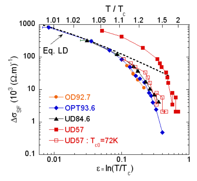
The variations of are reported versus in fig.6 for the four hole dopings studied. Except for the UD57 sample, it is striking to see that our experimental data collapse on a single curve and can be reasonably fitted by the LD expression (Eq.2) in the small temperature range if one takes Å. We have assumed here, as usually done, that the CuO2 bilayer constitutes the basic two-dimensional unit, and is then taken as the unit-cell size in the direction: Å. Based on these results, we have also analysed Nernst data previously measured in optimally doped YBCO crystals [10] along the same lines. In the GL approach, a simple relationship can be written between and the off-diagonal Peltier term as [14]:
| (4) |
A linear dependence can be indeed verified near between and whose slope results in a value of the zero temperature coherence length nm. Using , this would lead to T, a value very close to the result found below from the analysis of the magnetoconductivity. Consequently, one can conclude that, in optimally doped YBCO, the SCF contribution to the conductivity and the Nernst effect above can be interpreted in terms of Gaussian fluctuations only.
For the UD57 sample, is found to be about a factor four larger than for the other dopings. Quite surprisingly, it is possible to get a good matching with the data found for the other dopings by assuming a effective value different from the actual . This is illustrated by the empty symbols in fig.6 using K. This points to an additional origin of SCFs below which might be ascribed to phase fluctuations of the order parameter. This point is discussed in more details in ref.[7].
For all the samples, one can see in fig.6 that vanishes very rapidly for . This behaviour which has been noticed previously in many studies is particularly well defined here given the method used to extract the fluctuating conductivity. The cutoff which must be invoked to explain that behaviour implies that the density of fluctuating pairs vanishes at .
5 Field variation of the SCF conductivity: Onset field and upper critical field
From the data reported in Fig.2, we can extract the variation of with the applied magnetic field and analyse how the excess conductivity is destroyed by the field. This is reported in fig.7 for the optimally doped samples for between 107 and 130K.

Using the same criterion as defined above, we can thus determine the fields above which the signal is lower than 1 x . As decreases, it becomes difficult to ascertain that the normal state is fully reached when becomes comparable to the highest available field. This makes it difficult to precisely deduce values of larger than 45T.
The evolution of are plotted in fig.8 for the four samples. One can see that drops rapidly with increasing and displays a linear variation near . We have thus fitted the data using a parabolic variation as applied for the critical field of classical superconductors:
| (5) |
The fitting curves displayed as dashed lines in Fig.8 give correspondingly an indication of the field required to completely suppress the SC fluctuation contribution down to 0K. It is clear that increases with hole doping and reaches a value as high as Tesla at optimal doping.

A precise analysis of the fluctuation magnetoconductivity is a valuable tool to extract different microscopic parameters of high- cuprates, such as the value of not directly accessible from experiments. can be written out as:
| (6) | |||||
It has been very often assumed that the second term of the first equation can be neglected as being only weakly dependent on magnetic fields. However, our study clearly shows that this is not the case (see for instance the date displayed in fig.2). Thus our method provides here a correct determination of .
In the GL approach, the evolution of the fluctuation magnetoconductivity with comes from the pair-breaking effect which leads to a suppression. In the case of interest, the major contribution results from the AL process, and more particularly from the interaction of the field with the carrier orbital (ALO) degrees of freedom. The detailed analysis and discussion of the fluctuation magnetoconductivity are reported in ref.[7]. Fig.9 shows the data for the UD85 sample together with the fits using the ALO expression with T being the only adjustable parameter. We can checked that, as predicted by the theory, the fits are valid as long as . This latter field defined above mirrors the upper critical field and has been called the ”ghost critical field” by Kapitulnik et al [15].

The different values of extracted from the low-field part of the magnetoconductivity data are reported in table1. They are surprisingly very close to those obtained for in a completely different way. This gives strong weight to the consistency of our data analysis.
The important result here is to show that the superconducting gap which is directly related to increases smoothly with increasing hole doping from the underdoped to the overdoped regime, contrary to the pseudogap which decreases. This is a strong indication that the gap determined here can thus be assimilated to the ”small” gap detected recently by different techniques, while the pseudogap would be rather connected with the ”large” gap [5]
| Sample | UD57 | UD85 | OPT93.6 | OD92.5 |
|---|---|---|---|---|
| (T) | 90(10) | 125(5) | 180(10) | 200(10) |
| (T) | 86(10) | 115(5) | 155(10) | 207(10) |
6 Influence of disorder
It is now well admitted that the properties of cuprates are strongly dependent on disorder. We have studied for long the effect of the introduction of controlled disorder by electron irradiation and the way it affects the transport properties [16]. In particular, we have shown that similar upturns of the low-T resistivity are found for controlled disorder in YBCO and in some ”pure” low- cuprates, which indicates the existence of intrinsic disorder in those families [17].
We have also carried out magnetoresistance measurements in some OPT93.6 and UD57 samples irradiated by electrons. When is decreased by disorder, we find that both and are also affected. The reduction in nearly follows that in for the underdoped sample while it is slightly larger for the OPT sample. Consequently, when is decreased by disorder, the relative range of SCFs with respect to the value of expands considerably. For instance, we still detect K in an UD57 irradiated sample with K.
These results allow us to draw important conclusions on the cuprate phase diagram. Indeed, contrary to , or , the pseudogap temperature has been found very early to be quite robust to disorder [18]. This is another indirect evidence that the pseudogap phase is not related to superconductivity. We want also to emphasize here that specific effects induced by disorder are probably at the origin of many confusions in the study of high- cuprates. This leads us to propose in fig.10 a 3D phase diagram where the effect of disorder has been introduced as a third axis.

There, in the pure systems, the occurrence of SCFs and the difficulty to separate the SC gap from the pseudogap in zero-field experiments justifies that the line could often be taken as a continuation of the line.
It can also be seen in this figure that the respective evolutions with disorder of the SC dome and of the amplitude of the SCF range explains the phase diagram often shown in a low- cuprate such as Bi-2201 and sketched in fig.1(a). Finally, for intermediate disorder, the enhanced fluctuation regime with respect to observed in the Nernst measurements for the La2-xSrxCuO4 can be reproduced as well [4].
7 Conclusion
We have presented here a thorough quantitative study of the SCFs which establishes that such data give important determinations of some thermodynamic properties of the SC state of high- cuprates. Those are not accessible otherwise, as flux flow dominates near in the vortex liquid phase and the highest fields available so far are not sufficient to reach the normal state at . It has allowed us to demonstrate that the pairing energy and SC gap both increase with doping, confirming then that the pseudogap has to be assigned to an independent magnetic order or crossover due to the magnetic correlations.
Acknowledgements.
We thank D. Colson and A. Forget for providing the single crystals used in this work. We acknowledge collaboration with C. Proust, B. Vignolle and G. Rikken at the LNCMI. This work has been performed within the ”Triangle de la Physique” and was supported by ANR grant ”OXYFONDA” NT05-4 41913. The experiments at LNCMI-Toulouse were funded by the FP7 I3 EuroMagNET.References
- (1) H. Alloul, T. Ohno and P. Mendels, Phys. Rev. Lett. 63, (1989) 1700.
- (2) T. Timusk and B.Statt, Rep. Prog. Phys. 62 (1999) 61.
- (3) V.J. Emery and S.A Kivelson, Nature 374, 434 (1995).
- (4) Y. Wang, L. Li and N.P. Ong, Phys. Rev. B 73, 024510 (2006).
- (5) S Hüfner, M A Hossain, A Damascelli and G A Sawatzky, Rep. Prog. Phys. 71 (2008) 062501.
- (6) F. Rullier-Albenque, H. Alloul, C. Proust, D. Colson, and A. Forget, Phys. Rev. Lett. 99, (2007) 027003.
- (7) F. Rullier-Albenque, H. Alloul, G. Rikken, Phys. Rev. B 84 (2011) 014522.
- (8) H. Alloul, F. Rullier-Albenque, B. Vignolle, D. Colson, and A. Forget, Europhys. Lett. 91 (2010) 37005.
- (9) A. Legris, F. Rullier-Albenque, E. Radeva and P. Lejay, J. Phys. I France 3, 1605 (1993).
- (10) F.Rullier-Albenque, R. Tourbot, H. Alloul, P. Lejay, D. Colson, and A. Forget,Phys. Rev. Lett. 96 (2006) 067002.
- (11) Yayu Wang, Lu Li, M. J. Naughton, G. D. Gu, S. Uchida, and N. P. Ong, Phys. Rev. Lett. 95, (2005) 247002.
- (12) For a review see A. Larkin and A.A. Varlamov, Theory of fluctuations in superconductors (Oxford University Press, Oxford, 2005).
- (13) W.E. Lawrence and S. Doniach, proceedings 12th International Conference on Low Temperature Physics, Kyoto 1970 (E. Kanda, Keigaku, Tokyo 1971) 361.
- (14) I. Ussishkin, S.L. Sondhi and D.A. Huse , Phys. Rev. Lett. 89 287001 (2002).
- (15) A. Kapitulnik, A. Palevski and G. Deutscher, J. Phys. C: Solid State Phys., 18 (1985) 1305.
- (16) F.Rullier-Albenque, H. Alloul, R. Tourbot, Phys. Rev. Lett. 91, 047001 (2003).
- (17) F. Rullier-Albenque, H. Alloul, F. Balakirev, C. Proust, Europhys. Lett. 81, 37008 (2008).
- (18) H. Alloul, P. Mendels, H. Casalta, J.F. Marucco, and J. Arabski, Phys. Rev. Lett. 67(1991) 3140.