跳到论文正文
W Papers独立论文阅读器 arXiv:1205.1293 论文正文 计算阅读时间 · 0%
引用这篇论文根据当前论文元数据生成,正式投稿前建议核对。


License: arXiv.org perpetual non-exclusive license
arXiv:1205.1293v1 [math.NA] 07 May 2012

# FreeFem ++ , a tool to solve PDEs numerically

Georges Sadaka Affiliation: LAMFA CNRS UMR 7352 Affiliation: Université de Picardie Jules Verne Affiliation: 33, rue Saint-Leu, 80039 Amiens, France Affiliation: http://lamfa.u-picardie.fr/sadaka/ Email: 🖄 georges.sadaka@u-picardie.fr
Abstract

# FreeFem ++ is an open source platform to solve partial differential equations numerically, based on finite element methods. It was developed at the Laboratoire Jacques-Louis Lions, Université Pierre et Marie Curie, Paris by Frédéric Hecht in collaboration with Olivier Pironneau, Jacques Morice, Antoine Le Hyaric and Kohji Ohtsuka.

The

# FreeFem ++ platform has been developed to facilitate teaching and basic research through prototyping.

# FreeFem ++ has an advanced automatic mesh generator, capable of a posteriori mesh adaptation; it has a general purpose elliptic solver interfaced with fast algorithms such as the multi-frontal method UMFPACK, SuperLU . Hyperbolic and parabolic problems are solved by iterative algorithms prescribed by the user with the high level language of

# FreeFem ++ . It has several triangular finite elements, including discontinuous elements. For the moment this platform is restricted to the numerical simulations of problems which admit a variational formulation.

We will give in the sequel an introduction to

# FreeFem ++ which include the basic of this software. You may find more information throw this link http://www.freefem.org/ff++.

1 Introduction

# FreeFem ++ is a Free software to solve PDE using the Finite element method and it run on Mac, Unix and Window architecture.

In

# FreeFem ++ , it’s used a user language to set and control the problem. This language allows for a quick specification of linear PDE’s, with the variational formulation of a linear steady state problem and the user can write they own script to solve non linear problem and time depend problem.

It’s a interesting tool for the problem of average size. It’s also a help for the modeling in the sense where it allows to obtain quickly numerical results which is useful for modifying a physical model, to clear the avenues of Mathematical analysis investigation, etc …

A documentation of

# FreeFem ++ is accessible on www.freefem.org/ff++, on the following link www.freefem.org/ff++/ftp/FreeFem++doc.pdf, you may also have a documentation in spanish on the following link http://www.freefem.org/ff++/ftp/freefem++Spanish.pdf

You can also download an integrated environment called

# FreeFem ++ -cs, written by Antoine Le Hyaric on the following link www.ann.jussieu.fr/~lehyaric/ffcs/install.php

2 Characteristics of FreeFem++

Many of

# FreeFem ++ characteristics are cited in the full documentation of

# FreeFem ++ , we cite here some of them :

  • —

    Multi-variables, multi-equations, bi-dimensional and three-dimensional static or time dependent, linear or nonlinear coupled systems; however the user is required to describe the iterative procedures which reduce the problem to a set of linear problems.

  • —

    Easy geometric input by analytic description of boundaries by pieces, with specification by the user of the intersection of boundaries.

  • —

    Automatic mesh generator, based on the Delaunay-Voronoi algorithm [LucPir98].

  • —

    load and save Mesh, solution.

  • —

    Problem description (real or complex valued) by their variational formulations, the write of the variational formulation is too close for that written on a paper.

  • —

    Metric-based anisotropic mesh adaptation.

  • —

    A large variety of triangular finite elements : linear, quadratic Lagrangian elements and more, discontinuous P1 and Raviart-Thomas elements, …

  • —

    Automatic Building of Mass/Rigid Matrices and second member.

  • —

    Automatic interpolation of data from a mesh to an other one, so a finite element function is view as a function of (x; y) or as an array.

  • —

    LU, Cholesky, Crout, CG, GMRES, UMFPack sparse linear solver.

  • —

    Tools to define discontinuous Galerkin finite element formulations P0, P1dc, P2dc and keywords: jump, mean, intalledges.

  • —

    Wide range of examples : Navier-Stokes, elasticity, fluid structure, eigenvalue problem, Schwarz’ domain decomposition algorithm, residual error indicator, …

  • —

    Link with other software : modulef, emc2, medit, gnuplot, …

  • —

    Generates Graphic/Text/File outputs.

  • —

    A parallel version using mpi.

3 How to start?

All this information here are detailed in the

# FreeFem ++ documentation.

3.1 Install

First open the following web page

http://www.freefem.org/ff++/

Choose your platform: Linux, Windows, MacOS X, or go to the end of the page to get the full list of downloads and then install by double click on the appropriate file.

3.2 Text editor

  1. 1.

    For Windows :
    Install notepad++ which is available at http://notepad-plus.sourceforge.net/uk/site.htm

    • —

      Open Notepad++ and Enter F5

    • —

      In the new window enter the command FreeFem++ "$(FULL_CURRENT_PATH)"

    • —

      Click on Save, and enter FreeFem++ in the box ”Name”, now choose the short cut key to launch directly FreeFem++ (for example alt+shift+R)

    • —

      To add Color Syntax Compatible with FreeFem++ In Notepad++,

      • —

        In Menu "Parameters"->"Configuration of the Color Syntax" proceed as follows:

      • —

        In the list "Language" select C++

      • —

        Add ”edp” in the field "add ext"

      • —

        Select "INSTRUCTION WORD" in the list "Description" and in the field "supple mentary key word", cut and past the following list:

        P0 P1 P2 P3 P4 P1dc P2dc P3dc P4dc RT0 RT1 RT2 RT3 RT4 macro plot int1d int2d solve movemesh adaptmesh trunc checkmovemesh on func buildmesh square Eigenvalue min max imag exec LinearCG NLCG Newton BFGS LinearGMRES catch try intalledges jump average mean load savemesh convect abs sin cos tan atan asin acos cotan sinh cosh tanh cotanh atanh asinh acosh pow exp log log10 sqrt dx dy endl cout

      • —

        Select ”TYPE WORD” in the list ”Description” and … ” ”supplementary key word”, cut and past the following list

        mesh real fespace varf matrix problem string border complex ifstream ofstream

      • —

        Click on Save & Close. Now nodepad++ is configured.

  2. 2.

    For MacOS :
    Install Smultron which is available at http://smultron.sourceforge.net. It comes ready with color syntax for .edp file. To teach it to launch

    # FreeFem ++ files, do a ”command B” (i.e. the menu Tools/Handle Command/new command) and create a command which does

     /usr/local/bin/FreeFem++-CoCoa %%p
     
    
  3. 3.

    For Linux :
    Install Kate which is available at ftp://ftp.kde.org/pub/kde/stable/3.5.10/src/kdebase-3.5.10.tar.bz2

    To personalize with color syntax for .edp file, it suffices to take those given by Kate for c++ and to add the keywords of

    # FreeFem ++ . Then, download edp.xml and save it in the directory ”.kde/share/apps/katepart/syntax”.

    We may find other description for other text editor in the full documentation of

    # FreeFem ++ .

3.3 Save and run

All

# FreeFem ++ code must be saved with file extension .edp and to run them you may double click on the file on MacOS or Windows otherwise we note that this can also be done in terminal mode by : FreeFem++ mycode.edp

4 Syntax and some operators

4.1 Data types

In essence

# FreeFem ++ is a compiler: its language is typed, polymorphic, with exception and reentrant. Every variable must be declared of a certain type, in a declarative statement; each statement are separated from the next by a semicolon “;”.
Another trick is to comment in and out by using the “//” as in C++. We note that, we can also comment a paragraph by using “/* paragraph */” and in order to make a break during the computation, we can use “exit(0);”.
The variable verbosity changes the level of internal printing (0, nothing (unless there are syntax errors), 1 few, 10 lots, etc. …), the default value is 2 and the variable clock() gives the computer clock.
The language allows the manipulation of basic types :

  • —

    current coordinates : x, y and z;

  • —

    current differentials operators : dx=∂∂x=\displaystyle\frac{\partial}{\partial x}, dy=∂∂y=\displaystyle\frac{\partial}{\partial y}, dz=∂∂z=\displaystyle\frac{\partial}{\partial z}, dxy=∂∂x​y=\displaystyle\frac{\partial}{\partial xy}, dxz=∂∂x​z=\displaystyle\frac{\partial}{\partial xz}, dyz=∂∂y​z=\displaystyle\frac{\partial}{\partial yz}, dxx=∂∂x​x=\displaystyle\frac{\partial}{\partial xx}, dyy=∂∂y​y=\displaystyle\frac{\partial}{\partial yy} and dzz=∂∂z​z=\displaystyle\frac{\partial}{\partial zz};

  • —

    integers, example : int a=1;

  • —

    reals, example : real b=1.; (don’t forget to put a point after the integer number)

  • —

    complex, example : complex c=1.+3i;

  • —

    strings, example : string test="toto";

  • —

    arrays with real component, example: real[int] V(n); where n is the size of V,

  • —

    arrays with complex component, example: complex[int] V(n);

  • —

    matrix with real component, example: real[int,int] A(m,n);

  • —

    matrix with complex component, example: complex[int,int] C(m,n);

  • —

    bidimensional (2D) finite element meshes, example : mesh Th;

  • —

    2D finite element spaces, example : fespace Vh(Th,P1); // where Vh is the Id space

  • —

    threedimensional (3D) finite element meshes, example : mesh3 Th3;

  • —

    3D finite element spaces, example : fespace Vh3(Th3,P13d);

  • —

    int1d(Th,Γ\Gamma)( u*v ) =∫Γu⋅v​𝑑x=\displaystyle\int_{\Gamma}u\cdot v\,dx where Γ⊂ℝ\Gamma\subset\mathbb{R};

  • —

    int2d(Th)( u*v ) =∫Ωu⋅v​𝑑x​𝑑y=\displaystyle\int_{\Omega}u\cdot v\,dxdy where Ω⊂ℝ2\Omega\subset\mathbb{R}^{2};

  • —

    int3d(Th)( u*v ) =∫Ωu⋅v​𝑑x​𝑑y​𝑑z=\displaystyle\int_{\Omega}u\cdot v\,dxdydz where Ω⊂ℝ3\Omega\subset\mathbb{R}^{3}.

4.2 Some operators

We cite here some of the operator that are defined in

# FreeFem ++ :

+, -, *, /, ^,
<, >, <=, >=,
&, |, // where a & b = a and b, a | b = a or b
=, +=, -=, /=, *=, !=, ==.

4.3 Manipulation of functions

We can define a function as :

  • —

    an analytical function, example : func u0=exp(-x∧2-y∧2),u1=1.*(x>=-2 & x<=2);

  • —

    a finite element function or array, example : Vh u0=exp(-x∧2-y∧2);.
    We note that, in this case u0 is a finite element, thus u0[] return the values of u0 at each degree of freedom and to have access to the ithi^{{\small\mbox{th}}} element of u0[] we may use u0[][i].
    We can also have an access to the value of u0 at the point (a,b) by using u0(a,b);

  • —

    a complex value of finite element function or array, example : Vh<complex> u0=x+1i*y;

  • —

    a formal line function, example : func real g(int a, real b) { .....; return a+b;} and to call this function for example we can use g(1,2).
    We can also put an array inside this function as :

    func real f(int a, real[int] U){
    Vh NU;
    NU[]=U;
    return a*NU;
    }
    Vh U=x,FNU=f(5,U[]);
  • —

    macro function, example : macro F(t,u,v)[t*dx(u),t*dy(v)]//, notice that every macro must end by “//”, it simply replaces the name F(t,u,v) by [t*dx(u),t*dy(v)] and to have access only to the first element of F, we can use F(t,u,v)[0].

    In fact, we note that the best way to define a function is to use macro function since in this example t,u and v could be integer, real, complex, array or finite element, …
    For example, here is the most used function defined by a macro :

    macro Grad(u)[dx(u),dy(u)]// in 2D
    macro Grad(u)[dx(u),dy(u),dz(u)]// in 3D
    macro div(u,v)[dx(u)+dy(v)]// in 2D
    macro div(u,v,w)[dx(u)+dy(v)+dz(w)]// in 3D

4.4 Manipulation of arrays and matrices

Like in matlab, we can define an array such as : real[int] U=1:2:10; which is an array of 5 values U[i]=2*i+1; i=0 to 4 and to have access to the ithi^{{\small\mbox{th}}} element of U we may use U(i).

Also we can define a matrix such as real[int,int] A=[ [1,2,3] , [2,3,4] ]; which is a matrix of size 2×32\times 3 and to have access to the (i,j)th(i,j)^{{\small\mbox{th}}} element of A we may use A(i,j).

We will give here some of manipulation of array and matrix that we can do with

# FreeFem ++ :

real[int] u1=[1,2,3],u2=2:4; // defining u1 and u2
real u1pu2=u1’*u2; // give the scalar product of u1 and u2, here u1’ is the transpose of u1;
real[int] u1du2=u1./u2; // divided term by term
real[int] u1mu2=u1.*u2; // multiplied term by term
matrix A=u1*u2’; // product of u1 and the transpose of u2
matrix<complex> C=[ [1,1i],[1+2i,.5*1i] ];
real trA=trace([1,2,3]*[2,3,4]’); // trace of the matrix
real detA=det([ [1,2],[-2,1] ]); // just for matrix 1x1 and 2x2

4.5 Loops and conditions

The for and while loops are implemented in

# FreeFem ++ together with break and continue keywords.
In for-loop, there are three parameters; the INITIALIZATION of a control variable, the CONDITION to continue, the CHANGE of the control variable. While CONDITION is true, for-loop continue.

for (INITIALIZATION; CONDITION; CHANGE)
{ BLOCK of calculations }

An example below shows a sum from 1 to 10 with result is in sum,

int sum=0;
for (int i=1; i<=10; i++)
sum += i;

The while-loop

while (CONDITION) {
BLOCK of calculations or change of control variables
}

is executed repeatedly until CONDITION become false. The sum from 1 to 5 can also be computed by while, in this example, we want to show how we can exit from a loop in midstream by break and how the continue statement will pass the part from continue to the end of the loop :

int i=1, sum=0;
while (i<=10) {
sum += i; i++;
if (sum>0) continue;
if (i==5) break;
}

4.6 Input and output data

The syntax of input/output statements is similar to C++ syntax. It uses cout, cin, endl, << and >> :

int i;
cout << " std-out" << endl;
cout << " enter i= ? ";
cin >> i ;
Vh uh=x+y;
ofstream f("toto.txt"); f << uh[]; // to save the solution
ifstream f("toto.txt"); f >> uh[]; // to read the solution

We will present in the sequel, some useful script to use the

# FreeFem ++ data with other software such as ffglut, Gnuplot11 1 http://www.gnuplot.info/, Medit22 2 http://www.ann.jussieu.fr/~frey/software.html, Matlab33 3 http://www.mathworks.fr/products/matlab/, Mathematica44 4 http://www.wolfram.com/mathematica/, Visit55 5 https://wci.llnl.gov/codes/visit/ when we save data with extension as .eps, .gnu, .gp, .mesh, .sol, .bb, .txt and .vtu.
For ffglut which is the visualization tools through a pipe of

# FreeFem ++ , we can plot the solution and save it with a .eps format such as :

plot(uh,cmm="t="+t+" ;||u||_L^2="+NORML2[kk], fill=true,value=true,dim=2);
Refer to caption
Figure 1: Visualising of the solution using ffglut

For Gnuplot, we can save the data with extension .gnu or .gp such as :

{ ofstream gnu("plot.gnu"); // or plot.gp
//ofstream gnu("plot."+1000+k".gnu"); // to save the data
for (int i=0;i<=n;i++)
gnu<<xx[i]<<" "<<yy[i]<<endl; // to plot yy[i] vs xx[i]
}
exec("echo ’plot \"plot.gnu\" w lp \
pause 5 \
quit’ | gnuplot");

For Medit, we can save the data with extension .mesh and .sol such as :

load "medit"
int k=0;
savemesh(Th,"solution."+(1000+k)+".mesh");
savesol("solution."+(1000+k)+".sol",Th,uh);
medit("solution",Th,uh); // to plot the solution here
k+=1;

And then throw a terminal, in order to visualize the movie of the first 11 saved data, we can type this line :

ffmedit -a 1000 1010 solution.1000.sol

Don’t forget in the window of Medit, to click on “m” to visualize the solution!

Refer to caption
Figure 2: Visualising of the solution using Medit

For Matlab, we can save the data with extension .bb such as :

{ ofstream file("solution.bb");
file << "2 1 1 "<< Vh.ndof << " 2 \n";
for (int j=0;j<Vh.ndof ; j++)
file << uh[][j] << endl;
}

And in order to visualize with Matlab, you can see the script made by Julien Dambrine at http://www.downloadplex.com/Publishers/Julien-Dambrine/Page-1-0-0-0-0.html.

Refer to captionRefer to caption
Figure 3: Visualising of the solution and the mesh using matlab

For Mathematica, we can save the data with extension .txt such as :

int k=0;
{ ofstream ff("uhsol."+(1000+k)+".txt");
for (int i=0;i<Th.nt;i++){
for (int j=0; j <3; j++)
ff<<Th[i][j].x<<" "<< Th[i][j].y<<" "<<uh[][Vh(i,j)]<<endl;
ff<<Th[i][0].x<<" "<< Th[i][0].y<<" "<<uh[][Vh(i,0)]<<"\n";
}
}
k+=1;
Refer to caption
Figure 4: Visualising of the solution using Mathematica

For Visit, we can save the data with extension .vtu such as :
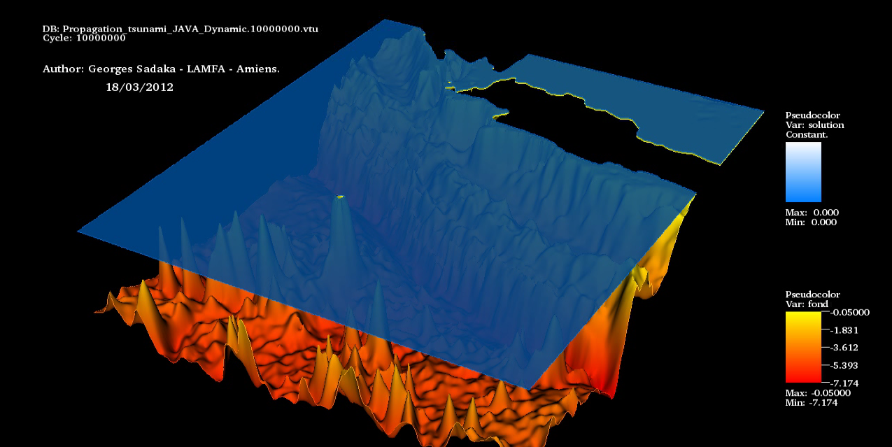
load "iovtk"
int k=0;
int[int] fforder2=[1,1,1];
savevtk("solution."+(1000+k)+".vtu",Th,uh1,uh2,order=fforder2,dataname="UH1 UH2", bin=true);
k+=1;
Refer to caption
Figure 5: Visualising of the solution using visit

5 Construction of the domain Ω\Omega

We note that in

# FreeFem ++ the domain is assumed to described by its boundary that is on the left side of the boundary which is implicitly oriented by the parametrization.
Let Ω\Omega be the rectangle defined by its frontier ∂Ω=[−5,5]×[−1,1]\partial\Omega=[-5,5]\times[-1,1] where his vertices are A⁡(−5,−1),B⁡(5,−1),C⁡(5,1)A(-5,-1),B(5,-1),C(5,1) and D⁡(−5,1)D(-5,1), so we must define the border A​B,B​C,C​DAB,BC,CD and D​ADA of ∂Ω\partial\Omega by using the keyword border then the triangulation 𝒯h\mathcal{T}_{h} of Ω\Omega is automatically generated by using the keyword buildmesh.

real Dx=.2; // discretization space parameter
int aa=-5,bb=5,cc=-1,dd=1;
border AB (t = aa, bb){x = t ;y = cc;label = 1;};
border BC (t = cc, dd){x = bb;y = t ;label = 2;};
border CD (t = bb, aa){x = t ;y = dd;label = 3;};
border DA (t = dd, cc){x = aa;y = t ;label = 4;};
mesh Th = buildmesh( AB(floor(abs(bb-aa)/Dx)) + BC(floor(abs(dd-cc)/Dx)) + CD(floor(abs(bb-aa)/Dx)) + DA(floor(abs(dd-cc)/Dx)) );
plot( AB(floor(abs(bb-aa)/Dx)) + BC(floor(abs(dd-cc)/Dx)) + CD(floor(abs(bb-aa)/Dx)) + DA(floor(abs(dd-cc)/Dx)) ); // to see the border
plot ( Th, ps="mesh.eps"); // to see and save the mesh

The keyword label can be added to define a group of boundaries for later use (Boundary Conditions for instance). Boundaries can be referred to either by name ( A​BAB for example) or by label ( 11 here).

Figure 6: Plot of the border (left) and the mesh (right)

Another way to construct a rectangle domain with isotropic triangle is to use :

mesh Th=square(m,n,[x,y]); // build a square with m point on x direction and n point on y direction
mesh Th1=movemesh(Th,[x+1,y*2]); // translate the square ]0,1[*]0,1[ to a rectangle ]1,2[*]0,2[
savemesh(Th1,"Name.msh"); // to save the mesh
mesh Th2("mesh.msh"); // to load the mesh
Figure 7: Boundary labels of the mesh by square(10,10)

We can also construct our domain defined by a parametric coordinate as:

border C(t=0,2*pi){ x=cos(t);y=sin(t);label=1}
mesh Mesh_Name=buildmesh(C(50));
Figure 8: mesh Th by build(C(50))

To create a domain with a hole we can proceed as:

border a(t=0,2*pi){ x=cos(t); y=sin(t);label=1;}
border b(t=0,2*pi){ x=0.3+0.3*cos(t); y=0.3*sin(t);label=2;}
mesh Thwithouthole= buildmesh(a(50)+b(+30));
mesh Thwithhole = buildmesh(a(50)+b(-30));
plot(Thwithouthole,wait=1,ps="Thwithouthole.eps");
plot(Thwithhole,wait=1,ps="Thwithhole.eps");
Figure 9: mesh without hole
Figure 10: mesh with hole

6 Finite Element Space

A finite element space (F.E.S) is, usually, a space of polynomial functions on elements of 𝒯h\mathcal{T}_{h}, triangles here, with certain matching properties at edges, vertices, … ; it’s defined as :

fespace Vh( Th, P1 );

As of today, the known types of F.E.S. are: P0, P03d, P1, P13d, P1dc, P1b, P1b3d, P2, P23d, P2b, P2dc, P3, P3dc, P4, P4dc, Morley, P2BR, RT0, RT03d, RT0Ortho, Edge03d, P1nc, RT1, RT1Ortho, BDM1, BDM1Ortho, TDNNS1; where for example:

P0,P03d

piecewise constant discontinuous finite element (2d, 3d), the degrees of freedom are the barycenter element value.

P0h={v∈L2(Ω)|for all K∈𝒯hthere is αK∈ℝ:v|K=αK}\displaystyle P0_{h}=\left\{v\in L^{2}(\Omega)\left|\;\textrm{for all }K\in\mathcal{T}_{h}\;\;\textrm{there is }\alpha_{K}\in\mathbb{R}:\;\;v_{|K}=\alpha_{K}\right.\right\} (1)
P1,P13d

piecewise linear continuous finite element (2d, 3d), the degrees of freedom are the vertices values.

P1h={v∈H1(Ω)|∀K∈𝒯h;v|K∈P1}\displaystyle P1_{h}=\left\{v\in H^{1}(\Omega)\left|\;\forall K\in\mathcal{T}_{h};\quad v_{|K}\in P_{1}\right.\right\} (2)

We can see the description of the rest of the F.E.S. in the full documentation of

# FreeFem ++ .

7 Boundary Condition

We will see in this section how it’s easy to define the boundary condition (B.C.) with

# FreeFem ++ , for more information about these B.C., we refer to the full documentation.

7.1 Dirichlet B.C.

To define Dirichlet B.C. on a border Γd⊂ℝ\Gamma_{d}\subset\mathbb{R} like u|Γd=fu|_{\Gamma_{d}}=f, we can proceed as on(gammad,u=f), where u is the unknown function in the problem. 
The meaning is for all degree of freedom ii of the boundary referred by the label “gammad”, the diagonal term of the matrix ai​i=t​g​va_{ii}=tgv with the terrible giant value t​g​vtgv (=103010^{30} by default) and the right hand side b⁡[i]="⁡(Πh​g)​[i]​"×t​g​vb[i]="(\Pi_{h}g)[i]"\times tgv, where the "⁡(Πh​g)​g​[i]​""(\Pi_{h}g)g[i]" is the boundary node value given by the interpolation of gg. (We are solving here the linear system A​X=BAX=B, where A=(ai​j)i=1..n;j=1..mA=\left(a_{ij}\right)_{i=1..n;j=1..m} and B=(bi)i=1..nB=\left(b_{i}\right)_{i=1..n} ).

If uu is a vector like u=(u​1,u​2)Tu=(u1,u2)^{T} and we have u​1|Γd=f​1u1|_{\Gamma_{d}}=f1 and u​2|Γd=f​2u2|_{\Gamma_{d}}=f2, we can proceed as on(gammad,u1=f1,u2=f2).

7.2 Neumann B.C.

The Neumann B.C. on a border Γn⊂ℝ\Gamma_{n}\subset\mathbb{R}, like ∂u∂n|Γn=g\displaystyle\frac{\partial u}{\partial n}|_{\Gamma_{n}}=g, appear in the Weak formulation of the problem after integrating by parts, for example ⟨∂u∂n;Φ⟩Γn=⟨g;Φ⟩Γn=∫Γng⋅Φ​𝑑x=\left\langle\displaystyle\frac{\partial u}{\partial n};\Phi\right\rangle_{\Gamma_{n}}=\left\langle g;\Phi\right\rangle_{\Gamma_{n}}=\displaystyle\int_{\Gamma_{n}}g\cdot\Phi\,dx= int1d(Th,gamman)(g*phi).

7.3 Robin B.C.

The Robin B.C. on a border Γr⊂ℝ\Gamma_{r}\subset\mathbb{R}; like a​u+κ​∂u∂n=bau+\kappa\displaystyle\frac{\partial u}{\partial n}=b on Γr\Gamma_{r} where a=a⁡(x,y)≥0a=a(x,y)\geq 0, κ=κ⁡(x,y)≥0\kappa=\kappa(x,y)\geq 0 and b=b⁡(x,y)b=b(x,y); also appear in the Weak formulation of the problem after integrating by parts, for example −⟨κ​∂u∂n;Φ⟩Γr=⟨a​u−b;Φ⟩Γr=∫Γra​u⋅Φ​𝑑x−∫Γrb⋅Φ​𝑑x=-\left\langle\kappa\displaystyle\frac{\partial u}{\partial n};\Phi\right\rangle_{\Gamma_{r}}=\left\langle au-b;\Phi\right\rangle_{\Gamma_{r}}=\displaystyle\int_{\Gamma_{r}}au\cdot\Phi\,dx-\displaystyle\int_{\Gamma_{r}}b\cdot\Phi\,dx= int1d(Th,gammar)(a*u*phi)-int1d(Th,gammar)(b*phi).

Important: it is not possible to write in the same integral the linear part and the bilinear part such as in int1d(Th,gammar)(a*u*phi-b*phi).

7.4 Periodic B.C.

In the case of Bi-Periodic B.C., they are achieved in the definition of the periodic F.E.S. such as :

fespace Vh( Th, P1,periodic=[[1,x],[3,x],[2,y],[4,y]] );

8 Solve the problem

We present here different way to solve the Poisson equation :
Find u:Ω=]0,1[×]0,1[⟶ℝu:\Omega=]0,1[\times]0,1[\longrightarrow\mathbb{R} such that, for a given f∈L2​(Ω)f\in L^{2}(\Omega):

{−Δ​u=f​in ​Ωu=0​ on ​∂Ω\left\{\begin{array}[]{rcl}-\Delta u&=&f\,\,\mbox{in }\Omega\\ u&=&0\,\mbox{ on }\,\partial\Omega\end{array}\right. (3)

Then the basic variational formulation of (3) is :
Find u∈H01​(Ω)u\in H_{0}^{1}(\Omega), such that for all v∈H01​(Ω)v\in H_{0}^{1}(\Omega),

a⁡(u,v)=l⁡(v)a(u,v)=l(v) (4)

where

a⁡(u,v)=∫Ω∇u⋅∇v​𝑑x​𝑑y​ and ​l​(v)=∫Ωf⋅v​𝑑x​𝑑ya(u,v)=\int_{\Omega}\nabla u\cdot\nabla v\,dxdy\mbox{ and }l(v)=\int_{\Omega}f\cdot v\,dxdy

To discretize (4), let 𝒯h\mathcal{T}_{h} denote a regular, quasi uniform triangulation of Ω\Omega with triangles of maximum size h<1h<1, let Vh={vh∈C0(Ω¯);vh|T∈ℙ1(T),∀T∈𝒯h;vh=0 on ∂Ω}V_{h}=\{v_{h}\in C^{0}(\bar{\Omega});v_{h}|_{T}\in\mathbb{P}_{1}(T),\forall T\in\mathcal{T}_{h};v_{h}=0\mbox{ on }\partial\Omega\} denote a finite-dimensional subspace of H01​(Ω)H_{0}^{1}(\Omega) where ℙ1\mathbb{P}_{1} is the set of polynomials of ℝ\mathbb{R} of degrees ≤1\leq 1.
Thus the discretize weak formulation of (4) is :

Find ​uh∈Vh:∫Ω∇uh⋅∇vh​𝑑x​𝑑y−∫Ωf⋅vh​𝑑x​𝑑y=0∀vh∈Vh.\mbox{Find }u_{h}\in V_{h}:\int_{\Omega}\nabla u_{h}\cdot\nabla v_{h}\,dxdy-\int_{\Omega}f\cdot v_{h}\,dxdy=0\qquad\forall v_{h}\in V_{h}. (5)

8.1 solve

The first method to solve (5) is to declare and solve the problem at the same time by using the keyword solve such as :

solve poisson(uh,vh,init=i,solver=LU) = // Solve Poisson Equation
int2d(Th)( Grad(uh)’*Grad(vh) ) // bilinear form
-int2d(Th)(f*vh) // linear form
+on(1,2,3,4,uh=0); // Dirichlet B.C.

The solver used here is Gauss’ LU factorization and when init ≠0\neq 0 the LU decomposition is reused so it is much faster after the first iteration. Note that if the mesh changes the matrix is reconstructed too.
The default solver is sparsesolver ( it is equal to UMFPACK if not other sparce solver is defined) or is set to LU if no direct sparse solver is available. The storage mode of the matrix of the underlying linear system depends on the type of solver chosen; for LU the matrix is sky-line non symmetric, for Crout the matrix is sky-line symmetric, for Cholesky the matrix is sky-line symmetric positive definite, for CG the matrix is sparse symmetric positive, and for GMRES, sparsesolver or UMFPACK the matrix is just sparse.

8.2 problem

The second method to solve (5) is to declare the problem by using the keyword problem, and then solve it later by just call his name, such as :

problem poisson(uh,vh,init=i,solver=LU)=// Definition of the problem
int2d(Th)( Grad(uh)’*Grad(vh) ) // bilinear form
-int2d(Th)(f*vh) // linear form
+on(1,2,3,4,uh=0); // Dirichlet B.C.
Poisson; // Solve Poisson Equation

Note that, this technique is used when we have a time depend problem.

8.3 varf

In

# FreeFem ++ , it is possible to define variational forms, and use them to build matrices and vectors and store them to speed-up the script.

The system (5) is equivalent to :

Find ​uh∈Vh:a⁡(uh,vh)=l⁡(vh)∀vh∈Vh.\mbox{Find }u_{h}\in V_{h}:a(u_{h},v_{h})=l(v_{h})\qquad\forall v_{h}\in V_{h}. (6)

Here,

uh​(x,y)=∑i=0M−1uhi​ϕi​(x,y)u_{h}(x,y)=\sum_{i=0}^{M-1}{u_{h}}_{i}\phi_{i}(x,y) (7)

where ϕi=vhi,i=0,…,M−1\phi_{i}={v_{h}}_{i},i=0,...,M-1 are the basis functions of VhV_{h}, M=M= Vh.ndof is the number of degree of freedom (i.e. the dimension of the space VhV_{h}) and uhiu_{h}{{}_{i}} is the value of uhu_{h} on each degree of freedom (i.e. uhi={u_{h}}_{i}=uh[][i]=UU).

Thus, using (7), we can rewrite (6) such as :

∑j=0M−1Ai​juhj−Fi=0,i=0,⋯,M−1;\sum_{j=0}^{M-1}A_{ij}{u_{h}}_{j}-F_{i}=0,\quad i=0,\cdots,M-1; (8)

where

Ai​j=∫Ω∇ϕj∇ϕidxdy and Fi=∫ΩfϕidxdyA_{ij}=\int_{\Omega}\nabla\phi_{j}\nabla\phi_{i}\,dxdy\qquad\mbox{ and }\qquad F_{i}=\int_{\Omega}f\phi_{i}\,dxdy

The matrix A=(Ai​j)A=(A_{ij}) is called stiffness matrix.
We deduce from the above notation that (8) is equivalent to

A⋅U=F⟺U=A−1⋅FA\cdot U=F\Longleftrightarrow U=A^{-1}\cdot F (9)

which can be solve in

# FreeFem ++ as :

int m=10,n=10;
mesh Th= square (m,n ,[x,y]);
fespace Vh( Th , P1 );
Vh uh,vh;
macro Grad (u)[dx(u),dy(u)]// in 2D
func f=1;
varf a(uh ,vh) = int2d (Th)( Grad (uh) ’* Grad (vh) ) // bilinear form
+on (1 ,2 ,3 ,4 , uh =0); // Dirichlet B.C.
matrix A=a(Vh ,Vh); // build the matrix
varf l( unused ,vh) = int2d (Th)(f*vh); // linear form
Vh F; F[] = l(0, Vh); // build the right hand side vector
set (A, solver = sparsesolver );
uh [] = A^ -1*F [];
plot(uh);

And in 3D :

load "msh3"
load "medit"
int m=10,n=10;
mesh Th2= square (m,n ,[x,y]);
mesh3 Th=buildlayers(Th2,10,zbound=[0,1]);
fespace Vh( Th , P13d );
Vh uh,vh;
macro Grad (u)[dx(u),dy(u),dz(u)]// in 2D
func f=1;
varf a(uh ,vh) = int3d (Th)( Grad (uh) ’* Grad (vh) ) // bilinear form
+on (0, 1 ,2 ,3 ,4 ,5 , uh =0); // Dirichlet B.C.
matrix A=a(Vh ,Vh); // build the matrix
varf l( unused ,vh) = int3d (Th)(f*vh); // linear form
Vh F; F[] = l(0, Vh); // build the right hand side vector
set (A, solver = sparsesolver );
uh [] = A^ -1*F [];
medit("sol",Th,uh);

9 Learning by examples

9.1 Rate of convergence for the Poisson equation

At the beginning, we prove that the rate of convergence in space for the Poisson equation code with P1P_{1} finite element is of order 2.
In this example, we took zero Dirichlet homogenous B.C. on the whole boundary and we have considered the following exact solution :

ue​x=sin⁡(π​x)⋅sin⁡(π​y)u_{ex}=\sin(\pi x)\cdot\sin(\pi y)

Then, we compute the corresponding right hand side f⁡(x,y)f(x,y) in order to obtain the L2L^{2} norm of the error between the exact solution and the numerical one (cf. Table 1)

E⁡(u,hn)=|uh​(hn)−ue​x​(hn)|L2,∀i=1,…,nref,h=δ​x=1/N;E(u,h_{n})=|u_{h}(h_{n})-u_{ex}(h_{n})|_{L^{2}},\forall i=1,...,\mbox{{nref}},h=\delta x=1/N;

and then the rate of convergence in space

r(u,hn)=log⁡(E⁡(u,hn−1)/E⁡(u,hn))log⁡(hn−1/hn),∀i=1,…,nrefr(u,h_{n})=\displaystyle\frac{\log\left(E(u,h_{n-1})/E(u,h_{n})\right)}{\log\left(h_{n-1}/h_{n}\right)},\forall i=1,...,\mbox{{nref}}

We give here a method to compute the right hand side using Maple66 6 http://www.maplesoft.com/ :

We can copy and paste the result of f⁡(x,y)f(x,y) in the

# FreeFem ++ code.
We present here the script to compute the rate of convergence in space of the code solving the Poisson equation :

int nref=4;
real[int] L2error(nref); // initialize the L2 error array
for (int n=0;n<nref;n++) {
int N=2^(n+4); // space discretization
mesh Th= square(N,N); // mesh generation of a square
fespace Vh(Th,P1); // space of P1 Finite Elements
Vh uh,vh; // uh and vh belongs to Vh
macro Grad(u)[dx(u),dy(u)]//
Vh uex=sin(pi*x)*sin(pi*y); // exact solution
Vh f=0.2e1*sin(pi*x)*pi^2*sin(pi*y); // corresponding RHS
varf a(uh,vh) = int2d(Th)( Grad(uh)’*Grad(vh) ) // bilinear form
+on(1,2,3,4,uh=0); // Dirichlet B.C.
matrix A=a(Vh,Vh); // build the matrix
varf l(unused ,vh) = int2d(Th)(f*vh); // linear form
Vh F; F[] = l(0,Vh); // build the right hand side vector
set(A,solver=sparsesolver);
uh[] = A^-1*F[];
L2error[n]= sqrt(int2d(Th)((uh-uex)^2));
}
for(int n=0;n<nref;n++)
cout << "L2error " << n << " = "<< L2error[n] <<endl;
for(int n=1;n<nref;n++)
cout <<"convergence rate = "<< log(L2error[n-1]/L2error[n])/log(2.) <<endl;
NnN_{n} E⁡(u,hn)E(u,h_{n}) r⁡(u,hn)r(u,h_{n})
16 0.0047854 -
32 0.00120952 1.9842
64 0.000303212 1.99604
128 7.58552e-05 1.99901
Table 1: L2L^{2} norm of the error and the rate of convergence.

9.2 Poisson equation over the Fila’s face

We present here a method to build a mesh from a photo using Photoshop®\circledR and a script in

# FreeFem ++ made by Frédéric Hecht.
We choose here to apply this method on the Fila’s face. To this end, we start by the photo in Figure 13, and using Photoshop®\circledR, we can remove the region that we wanted out of the domain such as in Figure 13, then fill in one color your domain and use some filter in Photoshop®\circledR in order to smooth the boundary as in Figure 13. Then convert your jpg photo to a pgm photo which can be read by

# FreeFem ++ by using in a terminal window :

convert fila.jpg fila.pgm
Refer to caption
Figure 11: Initial photo.
Refer to caption
Figure 12: Using Photoshop.
Refer to caption
Figure 13: Last photo.

Finally, using the following script :

load "ppm2rnm"
load "isoline"
string fila="fila.pgm";
real[int,int] Curves(3,1);
int[int] be(1);
int nc;
{ // build the curve file xy.txt ...
real[int,int] ff1(fila); // read image and set to an rect. array
// remark (0,0) is the upper, left corner.
int nx = ff1.n, ny=ff1.m;
// build a cartesain mesh such that the origne is qt the right place.
mesh Th=square(nx-1,ny-1,[(nx-1)*(x),(ny-1)*(1-y)]);
// warning the numbering is of the vertices (x,y) is
// given by $ i = x/nx + nx* y/ny $
fespace Vh(Th,P1);
Vh f1;
f1[]=ff1; // transforme array in finite element function.
real vmax = f1[].max ;
real vmin = f1[].min ;
real vm = (vmin+vmax)/2;
verbosity=3;
/*
Usage of isoline
the named parameter :
iso=0.25 // value of iso
close=1, // to force to have closing curve ...
beginend=be, // begin and end of curve
smoothing=.01, // nb of smoothing process = size^ratio * 0.01
where size is the size of the curve ...
ratio=0.5
file="filename"
ouptut:
xx, yy the array of point of the iso value
a closed curve number n is
in fortran notation the point of the curve are:
(xx[i],yy[i], i = i0, i1)
with : i0=be[2*n], i1=be[2*n+1];
*/
nc=isoline(Th,f1,iso=vm,close=0,Curves,beginend=be,smoothing=.005,ratio=0.1);
verbosity=1;
}
int ic0=be(0), ic1=be(1)-1;
plot([Curves(0,ic0:ic1),Curves(1,ic0:ic1)], wait=1);
// end smoothing the curve ....
macro GG(i)
border G#i(t=0,1)
{
P=Curve(Curves,be(i*2),be(i*2+1)-1,t);
label=i+1;
}
real lg#i=Curves(2,be(i*2+1)-1); //
GG(0) GG(1) GG(2) GG(3) GG(4) // number of closing curve
real hh= -10;
cout << " .. "<<endl;
func bord = G0(lg0/hh)+G1(lg1/hh)+G2(lg2/hh)+G3(lg3/hh)+G4(lg4/hh);
plot(bord,wait =1);
mesh Th=buildmesh(bord);
cout << " ... "<<endl;
plot(Th,wait=1);
Th=adaptmesh(Th,5.,IsMetric=1,nbvx=1e6);
plot(Th,wait=1);
savemesh(Th,"fila.msh");

we can create the mesh of our domain (cf. Figure 15), and then read this mesh in order to solve the Poisson equation on this domain (cf. Figure 15)

mesh Th("fila.msh");
plot(Th);
fespace Vh(Th,P1);
Vh uh,vh;
func f = 1.;
macro Grad(u)[dx(u),dy(u)]//
solve Poisson(uh,vh) = int2d(Th)(Grad(uh)’*Grad(vh)) - int2d(Th)( f*vh) + on(1,2,3,4,5,uh=0) ;
plot(uh,dim=2,fill=true,value=true);
Refer to caption
Figure 14: Mesh of the Fila’s face.
Refer to caption
Figure 15: Solution on the Fila’s face.

9.3 Rate of convergence for an Elliptic non linear equation

Let Ω=B⁡(O,R)⊂ℝ2\Omega=B(O,R)\subset\mathbb{R}^{2}, it is proposed to solve numerically the problem which consist to find u⁡(x,y)u(x,y) such that

{−Δ​u​(x,y)+u3=f for all ​(x,y)∈Ω⊂ℝ2,u⁡(x,y)=0 for all ​(x,y)​ on ​∂Ω.\displaystyle\left\{\begin{array}[]{rcl}-\Delta u(x,y)+u^{3}&=&f\quad\mbox{ for all }(x,y)\in\Omega\subset\mathbb{R}^{2},\\ u(x,y)&=&0\quad\mbox{ for all }(x,y)\mbox{ on }\partial\Omega.\end{array}\right.

9.3.1 Space discretization

Let 𝒯h\mathcal{T}_{h} be the triangulation of Ω\Omega and

Vh={vh∈C0(Ω¯);vh|T∈ℙ1(T),∀T∈𝒯h,vh=0 on ∂Ω}.V_{h}=\{v_{h}\in C^{0}(\bar{\Omega});v_{h}|_{T}\in\mathbb{P}_{1}(T),\forall T\in\mathcal{T}_{h},v_{h}=0\mbox{ on }\partial\Omega\}.

For simplicity, we denote by 𝒱⁡(u)=u2\mathcal{V}(u)=u^{2}, then the approximation of the variational formulation will be :
Find uh∈Vhu_{h}\in V_{h} such that ∀vh∈Vh\forall v_{h}\in V_{h} we have :

−⟨Δ​uh;vh⟩+⟨𝒱⁡(uh)⋅uh;vh⟩=⟨f;vh⟩-\left\langle\Delta u_{h};v_{h}\right\rangle+\left\langle\mathcal{V}(u_{h})\cdot u_{h};v_{h}\right\rangle=\left\langle f;v_{h}\right\rangle

thus

⟨∇uh;∇vh⟩+⟨𝒱⁡(uh)⋅uh;vh⟩=⟨f;vh⟩\left\langle\nabla u_{h};\nabla v_{h}\right\rangle+\left\langle\mathcal{V}(u_{h})\cdot u_{h};v_{h}\right\rangle=\left\langle f;v_{h}\right\rangle (13)

In order to solve numerically the non linear term in (17), we will use a semi-implicit scheme such as :

⟨∇uhn+1;∇vh⟩+⟨𝒱⁡(uhn)⋅uhn+1;vh⟩=⟨f;vh⟩,\left\langle\nabla u^{n+1}_{h};\nabla v_{h}\right\rangle+\left\langle\mathcal{V}(u^{n}_{h})\cdot u^{n+1}_{h};v_{h}\right\rangle=\left\langle f;v_{h}\right\rangle,

and then we solve our problem by the fixed point method in this way :

Set uh0=u0=0Set 𝒱⁡(uhn)=𝒱⁡(u0)Set e​r​r=1.while (e​r​r>1​e−10) Solve ​⟨∇uhp+1;∇vh⟩=−⟨𝒱⁡(uhn)⋅uhp;vh⟩+⟨f;vh⟩Compute ​e​r​r=‖uhn−uhp+1‖L2set ​𝒱​(uhn)=𝒱⁡(uhp+1)set ​uhn=uhp+1p=p+1;End while\begin{array}[]{ll}\mbox{\tt Set }&u^{0}_{h}=u_{0}=0\\ \mbox{\tt Set }&\mathcal{V}(u^{n}_{h})=\mathcal{V}(u_{0})\\ \mbox{\tt Set }&err=1.\\ \mbox{\tt while $(err>1e-10)$ }&\\ &\mbox{\tt Solve }\left\langle\nabla u^{p+1}_{h};\nabla v_{h}\right\rangle=-\left\langle\mathcal{V}(u^{n}_{h})\cdot u^{p}_{h};v_{h}\right\rangle+\left\langle f;v_{h}\right\rangle\\ &\mbox{\tt Compute }err=\|u^{n}_{h}-u^{p+1}_{h}\|_{L^{2}}\\ &\mbox{\tt set }\mathcal{V}(u^{n}_{h})=\mathcal{V}(u^{p+1}_{h})\\ &\mbox{\tt set }u^{n}_{h}=u^{p+1}_{h}\\ &p=p+1;\\ \mbox{\tt End while}&\end{array}

In order to test the convergence of this method we will study the rate of convergence in space (cf. Table 3) of the system (9.4) with R=1R=1 and the exact solution :

ue​x=sin⁡(x2+y2−1).u_{ex}=\sin(x^{2}+y^{2}-1).

Then, we compute the corresponding right hand side f⁡(x,y)f(x,y) using Maple such as :

We present here the corresponding script to compute the rate of convergence in space of the code solving the Elliptic non linear equation (9.4):

verbosity=0.;
int nraff=7;
real[int] L2error(nraff); // initialize the L2 error array
for (int n=0;n<nraff;n++) {
int N=2^(n+4); // space discretization
real R=1.; // radius
border C(t=0.,2.*pi){x=R*cos(t);y=R*sin(t);label=1;};
mesh Th=buildmesh(C(N));
fespace Vh(Th,P1);
Vh uh, uh0=0, V=uh0^2, vh;
Vh uex=sin((x ^ 2 + y ^ 2 - 1));
Vh f=0.4e1 * sin((x ^ 2 + y ^ 2 - 1)) * (x ^ 2) - 0.4e1 * cos((x ^ 2 + y ^ 2 - 1)) + 0.4e1 * sin((x ^ 2 + y ^ 2 - 1)) * (y ^ 2) + sin ((x ^ 2 + y ^ 2 - 1)) - sin((x ^ 2 + y ^ 2 - 1)) * cos((x ^ 2 + y ^ 2 - 1)) ^ 2;
macro Grad(u)[dx(u),dy(u)]//
problem ELLNL(uh,vh) =
int2d(Th)(Grad(uh)’*Grad(vh)) // bilinear term
+ int2d(Th) ( uh*V*vh ) // non linear term
- int2d(Th)( f*vh ) // right hand side
+ on(1,uh=0); // Dirichlet B.C.
real err=1.; // for the convergence
while (err >= 1e-10){
ELLNL;
err=sqrt(int2d(Th)((uh-uh0)^2));
V=uh^2; // actualization
uh0=uh;
}
L2error[n]= sqrt(int2d(Th)((uh-uex)^2));
}
for(int n=0;n<nraff;n++)
cout << "L2error " << n << " = "<< L2error[n] <<endl;
for(int n=1;n<nraff;n++)
cout <<"convergence rate = "<< log(L2error[n-1]/L2error[n])/log(2.) <<endl;
NnN_{n} E⁡(u,hn)E(u,h_{n}) r⁡(u,hn)r(u,h_{n})
16 0.015689 -
32 0.0042401 1.88758
64 0.00117866 1.84695
128 0.00032964 1.83819
256 8.48012e-05 1.95873
512 1.9631e-05 2.11095
1024 4.88914e-06 2.00548
Table 2: L2L^{2} norm of the error and the rate of convergence.

9.4 Rate of convergence for an Elliptic non linear equation with big Dirichlet B.C.

Let Ω=B⁡(O,R)⊂ℝ2\Omega=B(O,R)\subset\mathbb{R}^{2}, it is proposed to solve numerically the problem which consist to find u⁡(x,y)u(x,y) such that

{Δ​u​(x,y)=𝒱⁡(u)⋅u for all ​(x,y)∈Ω⊂ℝ2,u⁡(x,y)=D​B​C→+∞ for all ​(x,y)​ on ​∂Ω.\displaystyle\left\{\begin{array}[]{rcl}\Delta u(x,y)&=&\mathcal{V}(u)\cdot u\quad\mbox{ for all }(x,y)\in\Omega\subset\mathbb{R}^{2},\\ u(x,y)&=&DBC\rightarrow+\infty\quad\mbox{ for all }(x,y)\mbox{ on }\partial\Omega.\end{array}\right.

9.4.1 Space discretization

Let 𝒯h\mathcal{T}_{h} be the triangulation of Ω\Omega and

Vh={vh∈C0(Ω¯);vh|T∈ℙ1(T),∀T∈𝒯h,vh=p on ∂Ω},p⟶+∞.V_{h}=\{v_{h}\in C^{0}(\bar{\Omega});v_{h}|_{T}\in\mathbb{P}_{1}(T),\forall T\in\mathcal{T}_{h},v_{h}=p\mbox{ on }\partial\Omega\},p\longrightarrow+\infty.

Then the approximation of the variational formulation will be :
Find uh∈Vhu_{h}\in V_{h} such that ∀vh∈Vh\forall v_{h}\in V_{h} we have :

⟨Δ​uh;vh⟩=⟨𝒱⁡(uh)⋅uh;vh⟩\left\langle\Delta u_{h};v_{h}\right\rangle=\left\langle\mathcal{V}(u_{h})\cdot u_{h};v_{h}\right\rangle

thus

−⟨∇uh;∇vh⟩=⟨𝒱⁡(uh)⋅uh;vh⟩-\left\langle\nabla u_{h};\nabla v_{h}\right\rangle=\left\langle\mathcal{V}(u_{h})\cdot u_{h};v_{h}\right\rangle (17)

In order to solve numerically the non linear term in (17), we will use a semi-implicit scheme such as :

−⟨∇uhn+1;∇vh⟩=⟨𝒱⁡(uhn)⋅uhn+1;vh⟩,-\left\langle\nabla u^{n+1}_{h};\nabla v_{h}\right\rangle=\left\langle\mathcal{V}(u^{n}_{h})\cdot u^{n+1}_{h};v_{h}\right\rangle,

and then we solve our problem by the fixed point method in this way :

Set uh0=u0=D​B​C,p=0Set 𝒱⁡(uhn)=𝒱⁡(u0)Set e​r​r=1.while (e​r​r>1​e−10) Solve −⟨∇uhp+1;∇vh⟩=⟨𝒱⁡(uhn)⋅uhp;vh⟩Compute ​e​r​r=‖uhn−uhp+1‖L2set ​𝒱​(uhn)=𝒱⁡(uhp+1)p=p+1;End while\begin{array}[]{ll}\mbox{\tt Set }&u^{0}_{h}=u_{0}=DBC,p=0\\ \mbox{\tt Set }&\mathcal{V}(u^{n}_{h})=\mathcal{V}(u_{0})\\ \mbox{\tt Set }&err=1.\\ \mbox{\tt while $(err>1e-10)$ }&\\ &\mbox{\tt Solve }-\left\langle\nabla u^{p+1}_{h};\nabla v_{h}\right\rangle=\left\langle\mathcal{V}(u^{n}_{h})\cdot u^{p}_{h};v_{h}\right\rangle\\ &\mbox{\tt Compute }err=\|u^{n}_{h}-u^{p+1}_{h}\|_{L^{2}}\\ &\mbox{\tt set }\mathcal{V}(u^{n}_{h})=\mathcal{V}(u^{p+1}_{h})\\ &p=p+1;\\ \mbox{\tt End while}&\end{array}

In order to test the convergence of this method we will study the rate of convergence in space (cf. Table 3) for an application of (9.4), where R=1,𝒱⁡(u)=u,D​B​C=0R=1,\mathcal{V}(u)=u,DBC=0 or D​B​C=50DBC=50.
The system to be solved is then

Δ​u​(x,y)−u2\displaystyle\Delta u(x,y)-u^{2} =\displaystyle= f for all ​(x,y)∈Ω=B⁡(O,1)⊂ℝ2,\displaystyle f\quad\mbox{ for all }(x,y)\in\Omega=B(O,1)\subset\mathbb{R}^{2}, (18)
u⁡(x,y)\displaystyle u(x,y) =\displaystyle= D​B​C for all ​(x,y)​ on ​∂Ω.\displaystyle DBC\quad\mbox{ for all }(x,y)\mbox{ on }\partial\Omega. (19)

In this case, we will the following exact solution :

ue​x=D​B​C+sin⁡(x2+y2−1).u_{ex}=DBC+\sin(x^{2}+y^{2}-1).

Then, we compute the corresponding right hand side f⁡(x,y)f(x,y) using Maple such as :

We present here the corresponding script to compute the rate of convergence in space of the code solving the Elliptic non linear equation (18):

int nref=7;
real[int] L2error(nref); // initialize the L2 error array
for (int n=0;n<nref;n++) {
int N=2^(n+4); // space discretization
real R=1.; // radius
border C(t=0.,2.*pi){x=R*cos(t);y=R*sin(t);label=1;};
mesh Th=buildmesh(C(N));
fespace Vh(Th,P1);
real DBC=0.;
Vh uh, uh0=DBC, V=uh0, vh;
Vh uex=DBC+sin((x ^ 2 + y ^ 2 - 1));
Vh f=-0.4e1 * sin((x ^ 2 + y ^ 2 - 1)) * (x ^ 2) + 0.4e1 * cos((x ^ 2 + y ^ 2 - 1)) - 0.4e1 * sin((x ^ 2 + y ^ 2 - 1)) * (y ^ 2) - (DBC + sin((x ^ 2 + y ^ 2 - 1))) ^ 2;
macro Grad(u)[dx(u),dy(u)]//
problem ELLNL(uh,vh) =
- int2d(Th)(Grad(uh)’*Grad(vh)) // bilinear term
- int2d(Th) ( uh*V*vh ) // non linear term
- int2d(Th)( f*vh ) // right hand side
+ on(1,uh=DBC); // Dirichlet B.C.
real err=1.; // for the convergence
while (err >= 1e-10){
ELLNL;
err=sqrt(int2d(Th)((uh-V)^2));
V=uh; // actualization
}
L2error[n]= sqrt(int2d(Th)((uh-uex)^2));
}
for(int n=0;n<nref;n++)
cout << "L2error " << n << " = "<< L2error[n] <<endl;
for(int n=1;n<nref;n++)
cout <<"convergence rate = "<< log(L2error[n-1]/L2error[n])/log(2.) <<endl;
NnN_{n} E⁡(u,hn),E(u,h_{n}), DBC=0 r⁡(u,hn)r(u,h_{n}), DBC=0 E⁡(u,hn)E(u,h_{n}), DBC=50 r⁡(u,hn)r(u,h_{n}), DBC=50
16 0.0159388 - 0.00610357 -
32 0.00455562 1.80683 0.00244016 1.32268
64 0.00118025 1.94855 0.000767999 1.6678
128 0.000335335 1.81542 0.000210938 1.86429
256 8.6533e-05 1.95428 5.67798e-05 1.89337
512 1.9715e-05 2.13395 1.40771e-05 2.01203
1024 4.90847e-06 2.00595 3.56437e-06 1.98163
Table 3: L2L^{2} norm of the error and the rate of convergence.

9.5 Rate of convergence for the Heat equation

Let Ω=]0,1[2\Omega=]0,1[^{2}, we want to solve the Heat equation :

{∂u∂t−μ⋅Δ​u=f⁡(x,y,t) for all ​(x,y)∈Ω⊂ℝ2,t,μ∈ℝ+,u⁡(x,y,0)=u0​(x,y),u=0 on ​∂Ω.\displaystyle\left\{\begin{array}[]{rcl}\displaystyle\frac{\partial u}{\partial t}-\mu\cdot\Delta u&=&f(x,y,t)\quad\mbox{ for all }(x,y)\in\Omega\subset\mathbb{R}^{2},t,\mu\in\mathbb{R}^{+},\\ u(x,y,0)&=&u_{0}(x,y),\\ u&=&0\quad\mbox{ on }\partial\Omega.\end{array}\right.

9.5.1 Space discretization

Let 𝒯h\mathcal{T}_{h} be the triangulation of Ω\Omega and

Vh={vh∈C0(Ω¯);vh|T∈ℙ1(T),∀T∈𝒯h,vh=0 on ∂Ω}.V_{h}=\{v_{h}\in C^{0}(\bar{\Omega});v_{h}|_{T}\in\mathbb{P}_{1}(T),\forall T\in\mathcal{T}_{h},v_{h}=0\mbox{ on }\partial\Omega\}.

Then the approximation of the variational formulation will be :
Find uh∈Vhu_{h}\in V_{h} such that ∀vh∈Vh\forall v_{h}\in V_{h} we have :

⟨∂uh∂t;vh⟩−⟨μ⋅Δ​uh;vh⟩=⟨f;vh⟩\left\langle\frac{\partial u_{h}}{\partial t};v_{h}\right\rangle-\left\langle\mu\cdot\Delta u_{h};v_{h}\right\rangle=\left\langle f;v_{h}\right\rangle

Thus

⟨∂uh∂t;vh⟩+μ⋅⟨∇uh;∇vh⟩=⟨f;vh⟩\left\langle\frac{\partial u_{h}}{\partial t};v_{h}\right\rangle+\mu\cdot\left\langle\nabla u_{h};\nabla v_{h}\right\rangle=\left\langle f;v_{h}\right\rangle (24)

9.5.2 Time discretization

We will use here a θ\theta-scheme to discretize the Heat equation (24) as :

⟨uhn+1−uhnΔ​t;vh⟩+μ⋅θ⁡⟨∇uhn+1;∇vh⟩+μ⋅(1−θ)​⟨∇uhn;∇vh⟩=θ⋅⟨fn+1;vh⟩+(1−θ)⋅⟨fn;vh⟩.\left\langle\displaystyle\frac{u^{n+1}_{h}-u^{n}_{h}}{\Delta t};v_{h}\right\rangle+\mu\cdot\theta\left\langle\nabla u^{n+1}_{h};\nabla v_{h}\right\rangle+\mu\cdot(1-\theta)\left\langle\nabla u^{n}_{h};\nabla v_{h}\right\rangle=\theta\cdot\left\langle f^{n+1};v_{h}\right\rangle+(1-\theta)\cdot\left\langle f^{n};v_{h}\right\rangle.

Therefore :

⟨uhn+1Δ​t;vh⟩+μ⋅θ⁡⟨∇uhn+1;∇vh⟩=⟨uhnΔ​t;vh⟩−μ⋅(1−θ)​⟨∇uhn;∇vh⟩+θ⋅⟨fn+1;vh⟩+(1−θ)⋅⟨fn;vh⟩.\left\langle\displaystyle\frac{u^{n+1}_{h}}{\Delta t};v_{h}\right\rangle+\mu\cdot\theta\left\langle\nabla u^{n+1}_{h};\nabla v_{h}\right\rangle=\left\langle\displaystyle\frac{u^{n}_{h}}{\Delta t};v_{h}\right\rangle-\mu\cdot(1-\theta)\left\langle\nabla u^{n}_{h};\nabla v_{h}\right\rangle+\theta\cdot\left\langle f^{n+1};v_{h}\right\rangle+(1-\theta)\cdot\left\langle f^{n};v_{h}\right\rangle. (25)

To resolve (25) with

# FreeFem ++ , we will write it as a linear system of the form :

𝒜​X=ℬ⟺∑j=0M−1𝒜i,j⋅𝐗j=ℬi​ for ​i=0;…;M−1;\mathcal{A}\textbf{X}=\mathcal{B}\Longleftrightarrow\displaystyle\sum_{j=0}^{M-1}\mathcal{A}_{i,j}\cdot\mathbf{X}_{j}=\mathcal{B}_{i}\mbox{ for }i=0;\dots;M-1;

where, MM is the degree of freedom, the matrix 𝒜i,j\mathcal{A}_{i,j} and the arrays Xj\textbf{X}_{j} and ℬi\mathcal{B}_{i} are defining as :

Xj=uj,hn+1,𝒜i,j={t​g​v=1030if ​i∈∂Ω​ and ​j=i∫Ωφi​φjΔ​t+μ⋅θ⋅∇φi∇φjdxdyif ​j≠i\textbf{X}_{j}=u^{n+1}_{j,h},\qquad\mathcal{A}_{i,j}=\left\{\begin{array}[]{ll}tgv=10^{30}&\mbox{if }i\in\partial\Omega\mbox{ and }j=i\\ \displaystyle{\int_{\Omega}\frac{\varphi_{i}\varphi_{j}}{\Delta t}+\mu\cdot\theta\cdot\nabla\varphi_{i}\nabla\varphi_{j}dxdy}&\mbox{if }j\neq i\end{array}\right.
ℬi={t​g​v=1030if ​i∈∂Ω∫Ωuhn​φiΔ​t−μ⋅(1−θ)⋅∇unh∇φi+(θ⋅fn+1+(1−θ)⋅fn)φidxdyotherwise\mathcal{B}_{i}=\left\{\begin{array}[]{ll}tgv=10^{30}&\mbox{if }i\in\partial\Omega\\ \displaystyle{\int_{\Omega}\frac{u^{n}_{h}\varphi_{i}}{\Delta t}-\mu\cdot(1-\theta)\cdot\nabla u^{n}_{h}\nabla\varphi_{i}+\left(\theta\cdot f^{n+1}+(1-\theta)\cdot f^{n}\right)\varphi_{i}dxdy}&\mbox{otherwise}\end{array}\right.

We note that the θ\theta-scheme is stable under the CFL condition (when θ∈[0,1/2[\theta\in[0,1/2[) :

μ​Δ​tΔ​x+μ​Δ​tΔ​y≤12⋅(1−2​θ)\mu\displaystyle\frac{\Delta t}{\Delta x}+\mu\displaystyle\frac{\Delta t}{\Delta y}\leq\displaystyle\frac{1}{2\cdot(1-2\theta)}

In our test, we will consider that Δ​x=Δ​y\Delta x=\Delta y and that CFL∈]0,1]CFL\in]0,1], then when θ∈[0,1/2[\theta\in[0,1/2[, the θ\theta-scheme is stable under this condition :

Δ​t≤C​F​L⋅(Δ​x)24⋅μ⋅(1−2​θ),\Delta t\leq\displaystyle\frac{CFL\cdot(\Delta x)^{2}}{4\cdot\mu\cdot(1-2\theta)},

and for θ∈[1/2,1]\theta\in[1/2,1], the θ\theta-scheme is always stable.
We note also that due to the consistency error :

εi,jn≤c​Δ​t​|2​θ−1|+𝒪⁡(Δ​x2)+𝒪⁡(Δ​y2)+𝒪⁡(Δ​t2),\varepsilon_{i,j}^{n}\leq c\Delta t\left|2\theta-1\right|+\mathcal{O}\left(\Delta x^{2}\right)+\mathcal{O}\left(\Delta y^{2}\right)+\mathcal{O}\left(\Delta t^{2}\right),

the θ\theta-scheme is consistent of order 1 in time and 2 in space when θ=0\theta=0 (with the CFL condition) and when θ=1\theta=1 (with Δ​t=(Δ​x)2\Delta t=(\Delta x)^{2}) and the θ\theta-scheme is consistent of order 2 in time and in space when θ=1/2\theta=1/2 (with Δ​t=Δ​x\Delta t=\Delta x) (cf. Table 4).

Remark.

When we use finite element, mass lumping is usual with explicit time-integration schemes (as when θ∈[0,1/2[\theta\in[0,1/2[). It yields an easy-to-invert mass matrix at each time step, while improving the CFL condition [Hug87]. In

# FreeFem ++ , mass lumping are defined as int2d(Th,qft=qf1pTlump).

In order to test numerically the rate of convergence in space and in time of the θ\theta-scheme, we will consider the following exact solution :

ue​x=sin⁡(π​x)⋅sin⁡(π​y)​es​i​n​(t).u_{ex}=\sin(\pi x)\cdot\sin(\pi y)e^{sin(t)}.

Then, we compute the corresponding right hand side f⁡(x,y)f(x,y) using Maple such as :

we remind that the rate of convergence in time is

r(u,dtn,hn)=log⁡(E⁡(u,hn−1)/E⁡(u,hn))log⁡(d​tn−1/d​tn),∀n=1,…,nrefr(u,dt_{n},h_{n})=\displaystyle\frac{\log\left(E(u,h_{n-1})/E(u,h_{n})\right)}{\log\left(dt_{n-1}/dt_{n}\right)},\forall n=1,...,\mbox{{nref}}
macro Grad(u)[dx(u),dy(u)]//
macro uex(t) (sin(pi*x)*sin(pi*y)*exp(sin(t)))//
macro f(t) ( sin(pi * x) * sin(pi * y) * exp(sin(t)) * (cos(t) + 0.2e1 * mu * pi ^ 2) ) //
real t, dt, h,T=.1, mu=1., CFL=1., theta=0.;
int nref=4;
real[int] L2error(nref); // initialize the L2 error array
real[int] Dx(nref); // initialize the Space discretization array
real[int] DT(nref); // initialize the Time discretization array
for (int n=0;n<nref;n++) {
int N=2^(n+4);
t=0;
h=1./N;
Dx[n]=h;
if (theta<.5)
dt=CFL*h^2/4./(1.-2.*theta)/mu;
else if (theta==.5)
dt=h;
else
dt=h^2;
DT[n]=dt;
mesh Th=square(N,N);
fespace Vh(Th,P1);
Vh u,u0,B;
varf a(u,v) = int2d(Th,qft=qf1pTlump)(u*v/dt + Grad(u)’*Grad(v)*theta*mu) + on(1,2,3,4,u=0);
matrix A = a(Vh,Vh);
varf b(u,v) = int2d(Th,qft=qf1pTlump)(u0*v/dt - Grad(u0)’*Grad(v)*(1.-theta)*mu ) + int2d(Th,qft=qf1pTlump)( (f(t+dt)*theta+f(t)*(1.-theta))*v ) + on(1,2,3,4,u=0);
u=uex(t);
for (t=0;t<=T;t+=dt){
u0=u;
B[] = b(0,Vh);
set(A,solver=sparsesolver);
u[] = A^-1*B[];
}
L2error[n]=sqrt(int2d(Th)(abs(u-uex(t))^2));
}
for(int n=0;n<nref;n++)
cout << "L2error " << n << " = "<< L2error[n] <<endl;
for(int n=1;n<nref;n++){
cout <<"Space convergence rate = "<< log(L2error[n-1]/L2error[n])/log(Dx[n-1]/Dx[n]) <<endl;
cout <<"Time convergence rate = "<< log(L2error[n-1]/L2error[n])/log(DT[n-1]/DT[n]) <<endl;
}
NnN_{n} 16 32 64 128
E⁡(u,hn),θ=0E(u,h_{n}),\,\theta=0 0.00325837 0.000815303 0.000203872 5.09709e-05
r⁡(u,hn),θ=0r(u,h_{n}),\,\theta=0 - 1.99874 1.99967 1.99992
r⁡(u,d​tn,hn),θ=0r(u,dt_{n},h_{n}),\,\theta=0 - 0.99937 0.999834 0.99996
E⁡(u,hn),θ=1/2E(u,h_{n}),\,\theta=1/2 0.00325537 0.000819141 0.000203817 5.08854e-05
r⁡(u,hn),θ=1/2r(u,h_{n}),\,\theta=1/2 - 1.99064 2.00684 2.00195
r⁡(u,d​tn,hn),θ=1/2r(u,dt_{n},h_{n}),\,\theta=1/2 - 1.99064 2.00684 2.00195
E⁡(u,hn),θ=1E(u,h_{n}),\,\theta=1 0.00323818 0.000807805 0.000201833 5.04512e-05
r⁡(u,hn),θ=1r(u,h_{n}),\,\theta=1 - 2.0031 2.00084 2.0002
r⁡(u,d​tn,hn),θ=1r(u,dt_{n},h_{n}),\,\theta=1 - 1.00155 1.00042 1.0001
Table 4: L2L^{2} norm of the error and the rate of convergence in space and in time for different θ\theta.

10 Conclusion

We presented here a basic introduction to

# FreeFem ++ for the beginner with

# FreeFem ++ . For more information, go to the following link http://www.freefem.org/ff++.

Acknowledgements : This work was done during the CIMPA School - Caracas 16-27 of April 2012. I would like to thank Frédéric Hecht (LJLL, Paris), Antoine Le Hyaric (LJLL, Paris) and Olivier Pantz (CMAP, Paris) for fruitful discussions and remarks.

References

  • [Hug87] Thomas J. R. Hughes. The finite element method. Prentice Hall Inc., Englewood Cliffs, NJ, 1987. Linear static and dynamic finite element analysis, With the collaboration of Robert M. Ferencz and Arthur M. Raefsky. Remark
  • [LucPir98] Brigitte Lucquin and Olivier Pironneau. Introduction to Scientific Computing. Wiley, 1998. PDF. — ‣ 2