Nonequilibrium mode-coupling theory for uniformly sheared underdamped systems

Koshiro Suzuki Email: suzuki.koshiro@canon.co.jp Affiliation: Analysis Technology Development Center, Canon Inc., 30-2 Shimomaruko 3-chome, Ohta-ku, Tokyo 146-8501, Japan Hisao Hayakawa Affiliation: Yukawa Institute for Theoretical Physics, Kyoto University, Kitashirakawa Oiwake-cho, Kyoto 606-8502, Japan

August 24, 2026

Abstract

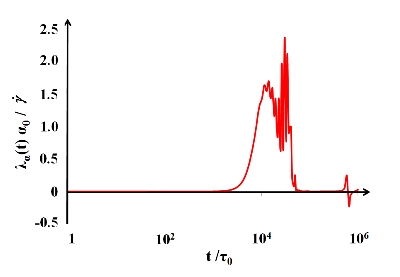
Nonequilibrium mode-coupling theory (MCT) for uniformly sheared underdamped systems is developed, starting from the microscopic thermostatted SLLOD equation, and the corresponding Liouville equation. Special attention is paid to the translational invariance in the sheared frame, which requires an appropriate definition of the transient time-correlators. The derived MCT equation satisfies the alignment of the wavevectors, and is manifestly translationally invariant. Isothermal condition is implemented by the introduction of the current fluctuation in the dissipative coupling to the thermostat. This current fluctation grows in the $\alpha$ -relaxation regime, which generates a deviation of the yield stress in the glassy phase from the overdamped case. Response to a perturbation of the shear rate demonstrates an inertia effect which is not observed in the overdamped case. Our theory turns out to be a non-trivial extension of the theory by Fuchs and Cates (J. Rheol. 53(4), 2009) to underdamped systems. Since our starting point is identical to that by Chong and Kim (Phys. Rev. E 79, 2009), the contradictions between Fuchs-Cates and Chong-Kim are resolved.

pacs

64.70.P-, 61.20.Lc, 83.50.Ax, 83.60.Fg

I Introduction

Liquids under shear are attracting continuous interest, not only for the importance of their application to industry, but also for their significance to the study of nonequilibrium statistical physics as ideal but experimentally accessible systems. Among them, special attention has been paid to dense supercooled liquids in the vicinity of the glass transition, i.e. glassy materials, due to their difficulty of understanding and their peculiarity compared with conventional systems which exhibit thermodynamic phase transitions.

Although not yet perfect, the mode-coupling theory (MCT) presents remarkable success in its application to glassy materials such as colloidal suspensions [1, 2, 3]. Probably the most striking feature of MCT is that it predicts a two-step relaxation phenomenon (the $\beta$ -relaxation followed by the $\alpha$ -relaxation) [4, 5] of the intermediate scattering function (i.e. density time-correlator) in the vicinity of a critical packing fraction $\varphi_{c}$ , which is referred to as the “MCT transition point”. This two-step relaxation is thoroughly investigated, and it is established that MCT is able to explain, e.g. the following properties: (i) square-root cusp anomaly of the temperature dependence of the plateau height of the density time-correlator (called the non-ergodic parameter, NEP) [6], (ii) power-law time-dependence with von Schweidler exponents of the density time-correlator around the $\beta$ -relaxation [7, 8, 9], (iii) time-temperature superposition principle realized by the Kohlrausch-Williams-Watts-type behavior of the density time-correlator at the $\alpha$ -relaxation [10]. On the other hand, MCT is marred with the problem that the NEP can survive for temperatures below the critical temperature $T_{c}$ , while it decays to zero in actual glassy states [4, 11]. Moreover, $\varphi_{c}$ is about 10% smaller than the experimental value. To overcome these difficulties, successive studies beyond the conventional MCT have been carried out eagerly as well, e.g. (i) field-theoretic formulations [12, 13, 14, 15, 16], (ii) inclusion of higher-order correlations [17, 18, 19], (iii) estimation of the dynamic correlation length [20].

The framework of MCT itself is generic, and extensions to other materials such as dense granular materials [21, 22, 23] have also been attempted. In particular, MCT is able to incorporate the effect of shear and its resulting demolition of the “cage effect”.

The introduction of shear into MCT has been worked out in the pioneering papers by Fuchs and Cates (FC) [24] and Miyazaki and Reichman [25], both of which have been formulated for sheared systems immersed in solvents, such as colloidal suspensions. The weak point of the approach of Ref. [25], which was followed by Ref. [21], has been pointed out by Chong and Kim (CK) [26]. They argued that the approach of Refs. [25, 21], where the steady-state structure factor (or, equivalently, the radial distribution function) is plugged in as an input, and then the steady-state shear stress is calculated as an output, is inconsistent, since they should be treated on the same footing. Rather, the equilibrium structure factor should be plugged in as an input, which is the case for Ref. [24]. (This scheme [27] is referred to as the “integration-through-transient (ITT)“ in Ref. [28].)

In this spirit, CK [26] have constructed MCT for a sheared system associated with a thermostat, where the SLLOD equation [27, 29] is chosen as a microscopic starting point. In contrast to the theory of FC [24, 28, 30], where a Brownian system governed by the Smoluchowski operator is the starting point, the SLLOD equation is governed by the Liouville operator (Liouvillian), and the momentum variables are left unintegrated, i.e. it is an underdamped system.

Besides this issue, apparent discrepancies between the resulting equations of CK [26] and FC [24, 28, 30] have been noticed. For instance, the “initial decay rate” of the Debye relaxation, which exhibits the conventional Taylor dispersion, is time-dependent in FC [24, 28, 30], while it is not in CK [26]. Probably the most notable difference is that there appears an additional memory kernel in CK [26], in addition to the conventional one which also appears commonly in other MCTs. As is well known, and is also argued in CK [26], these discrepancies cannot be the result of the difference of underdamped and overdamped systems, which exhibit quite similar behavior for long-time dynamics [31, 32, 33]. These contradictions were apparent, at least at the formal level, but as far as we know, no reconciliation has been proposed so far.

In this paper, we reformulate the MCT for uniformly sheared underdamped systems, and resolve the contradictions mentioned above. We point out that the definition of the time-correlators by CK [26] should be modified to satisfy the translational invariance in the sheared frame and fulfill the requirement of physical correlations between the Fourier modes of the fluctuations. This modification leads to complexities, which are absent in the formulation of CK [26], due to the non-commutativity and the non-Hermiticity of the Liouvillians. The path which handles these complexities closely follows that of FC [30], which we believe to be the most sensible so far ¹¹ 1 There is a subtle problem in defining the “random force” in the present formulation, as is also pointed out in Ref. [30]. This issue will be discussed in section V .

The crucial difference of our formulation to the CK’s is the introduction of the isothermal condition, which is implemented at the level of the Mori-type equations. This is realized by incorporating current fluctuations into the dissipative coupling to the thermostat, accompanied by the introduction of a multiplier. The growth of this fluctuation in the $\alpha$ -relaxation regime generates deviation of the yield stress in the glassy phase from that of the overdamped case. The resulting equation formally corresponds to that of FC [30] in the overdamped limit, but the effect of the inertia or the fluctuating coupling to the thermostat renders this correspondence to be highly non-trivial. Hence, our framework appears to be a non-trivial extension of FC [30] to underdamped systems. The significance of the underdamped formulation is also demonstrated by its application to the calculation of the response to a perturbation of the shear rate, where the inertia effect is clearly observed.

The paper is organized as follows. In section II, we briefly review the microscopic starting points. In section III, special attention is paid to the translational invariance in the sheared frame and the physically sensible definition of the time-correlators. Adjoint Liouvillians are introduced, which turns out to be natural in the treatment of sheared systems. In section IV, Mori-type equations are derived by the application of the projection operator formalism, first without the isothermal condition. After that, the isothermal condition is formulated, and the Mori-type equation where this condition is implemented is derived. In section V, the mode-coupling approximation is worked out, and a closed equation for the time-correlators (MCT equation) is derived. In section VI, a general formula of time-correlators for the steady-state quantities is presented, and the specific forms of the the dissipative coupling and the multiplier are discussed. A formula for the steady-state shear stress in this formulation is derived. In section VII, the result of the numerical calculation is shown for the density time-correlator and the steady-state shear stress, where the current fluctuation in the coupling to the thermostat plays an important role in the $\alpha$ -relaxation. The results of the CK theory [26] and the overdamped limit are also shown and are compared to the above result. In addition, response to a perturbation of the shear rate is shown. Section VIII is provided for discussion. Here, we first compare our work with the major preceding works. We hope that issues which were previously confusing are clarified. Then, the physical significance of the present formulation and the possibility of its extension are discussed. Finally, in section IX, we summarize our results and conclude the paper. An application to the response theory (Appendix A), comparison of the Mori-type equations in the underdamped and overdamped cases (Appendix B), and technical details (Appendices C and D) are collected in the Appendices.

II Microscopic starting points

Here we briefly summarize our microscopic starting points, i.e. the SLLOD equation, the Liouville equation, and the steady-state formula. Our treatment closely follows that of CK [26], so the details in common are to be referred to Ref. [26]. The crucial difference, however, is that our formulation is intended to satisfy the isothermal condition, which will be presented in section IV.4. Attentions related to this issue will be paid.

II.1 SLLOD equation

We deal with an assembly of $N$ equivalent spheres with diameter $d$ and mass $m$ , interacting with themselves and a thermostat in a volume $V$ . The interaction between the spheres is assumed to be a two-body soft-core potential force. Uniform shear is imposed on this system, where the shear velocity is given by ${\bm{v}}_{\mathrm{sh}}={\bm{\kappa}}\cdot{\bm{r}}$ . Here, ${\bm{\kappa}}$ is the time-independent shear-rate tensor, which is assumed to be of the form ${\bm{\kappa}}_{\mu\nu}=\dot{\gamma}\delta_{\mu x}\delta_{\nu y}$ in this paper, where the shear rate is denoted as $\dot{\gamma}$ . ${\bm{r}}$ is the spatial coordinate, and Greek indices $\lambda,\mu,\nu,\cdots$ denote spatial components $\{x,y,z\}$ in the remainder. We introduce the distance of the two shear boundaries, $L$ , for later convenience. Then, the shear velocity at the boundaries are $v_{0}^{(\pm)}\equiv\pm\dot{\gamma}L/2$ for $y=\pm L/2$ , respectively. The Newtonian equation of motion for the $i$ -th sphere ( $i=1,2,\cdots,N$ ) is given by the following SLLOD equation [27, 29],

	$\displaystyle\dot{{\bm{r}}}_{i}(t)$	$\displaystyle=$	$\displaystyle\frac{{\bm{p}}_{i}(t)}{m}+{\bm{\kappa}}\cdot{\bm{r}}_{i}(t),$		(1)
	$\displaystyle\dot{{\bm{p}}}_{i}(t)$	$\displaystyle=$	$\displaystyle{\bm{F}}_{i}(t)-{\bm{\kappa}}\cdot{\bm{p}}_{i}(t)-\alpha\left({\bm{\Gamma}}\right){\bm{p}}_{i}(t).$		(2)

Here, $\{{\bm{r}}_{i}(t),{\bm{p}}_{i}(t)\}$ is the position and the momentum of the $i$ -th sphere at time $t$ , and ${\bm{\Gamma}}(t)\equiv\{{\bm{r}}_{i}(t),{\bm{p}}_{i}(t)\}_{i=1}^{N}$ is the phase-space coordinate. In Eq. (1), ${\bm{p}}_{i}(t)$ is defined as a relative momentum in the sheared frame, and is referred to as the peculiar or the thermal momentum. ${\bm{F}}_{i}(t)\equiv-\partial U/\partial{\bm{r}}_{i}(t)=-\sum_{j}\partial u\left(r_{ij}(t)\right)/\partial{\bm{r}}_{ij}(t)$ is the conservative force acting on the $i$ -th sphere from other spheres, $U$ is the total potential, $u\left(r_{ij}(t)\right)$ is the two-body potential, ${\bm{r}}_{ij}(t)\equiv{\bm{r}}_{i}(t)-{\bm{r}}_{j}(t)$ is the relative position and $r_{ij}(t)\equiv|{\bm{r}}_{ij}(t)|$ is the relative distance, between the $i$ -th and $j$ -th spheres, respectively. The parameter $\alpha\left({\bm{\Gamma}}\right)$ represents the strength of the coupling of spheres to the thermostat, which in general implicitly depends on time through its dependence on ${\bm{\Gamma}}(t)$ . Note that $\alpha({\bm{\Gamma}})$ has been assumed to be a constant in Ref. [26]. It is possible to prevent the system from heating-up and control the kinetic temperature to be a constant by tuning the coupling $\alpha({\bm{\Gamma}})$ , in which case $\alpha({\bm{\Gamma}})$ should be regarded as a multiplier, rather than an independent physical parameter. A well-known example can be found in molecular dynamics, which is the Gaussian isokinetic (GIK) thermostat [27]. This thermostat is distinguished by its generality and its importance, which has the explicit time dependence as

\displaystyle\alpha(t)

\displaystyle=

\displaystyle\frac{\sum_{i}\left[{\bm{F}}_{i}(t)\cdot{\bm{p}}_{i}(t)-\dot{\gamma}p_{i}^{x}(t)p_{i}^{y}(t)\right]}{\sum_{j}{\bm{p}}_{j}(t)\cdot{\bm{p}}_{j}(t)},

(3)

which can be derived from the condition $\frac{d}{dt}\sum_{i}{\bm{p}}_{i}(t)^{2}=0$ . The specific form of $\alpha({\bm{\Gamma}})$ in MCT with isothermal condition will be discussed later in section VI.2. Note that Eqs. (1) and (2) reduce to Newtonian equations if we introduce the viscous force ${\bm{F}}_{i}^{(\mathrm{vis})}(t)\equiv-\alpha({\bm{\Gamma}})m\left(\dot{{\bm{r}}}_{i}(t)-{\bm{\kappa}}\cdot{\bm{r}}_{i}(t)\right)$ , except for the instant onset of the shear.

II.2 Liouville equation

The Liouville equation for a phase-space variable $A({\bm{\Gamma}}(t))$ reads

	$\displaystyle\frac{d}{dt}A\left({\bm{\Gamma}}(t)\right)$	$\displaystyle=$	$\displaystyle\dot{{\bm{\Gamma}}}({\bm{\Gamma}}(t))\cdot\left.\frac{\partial A({\bm{\Gamma}})}{\partial{\bm{\Gamma}}}\right\|_{{\bm{\Gamma}}={\bm{\Gamma}}(t)}$		(4)
		$\displaystyle=$	$\displaystyle e^{i\mathcal{L}t}i\mathcal{L}A\left({\bm{\Gamma}}(0)\right)=i\mathcal{L}A\left({\bm{\Gamma}}(t)\right),$		(4)

where the action of the Liouvillian $i\mathcal{L}$ is defined as

\displaystyle i\mathcal{L}A\left({\bm{\Gamma}}(0)\right)

\displaystyle\equiv

\displaystyle\dot{{\bm{\Gamma}}}({\bm{\Gamma}})\cdot\left.\frac{\partial A({\bm{\Gamma}}^{\prime})}{\partial{\bm{\Gamma}}^{\prime}}\right|_{{\bm{\Gamma}}^{\prime}={\bm{\Gamma}}}.

(5)

Here, and in the remainder, the abbreviated notation ${\bm{\Gamma}}\equiv{\bm{\Gamma}}(0)$ is adopted. The formal solution of Eq. (4) is given by $A\left({\bm{\Gamma}}(t)\right)=e^{i\mathcal{L}t}A\left({\bm{\Gamma}}\right)$ . Note that, in Eqs. (4) and (5), the Liouvillian is assumed not to bear explicit time-dependence. This is compatible with a time-independent shear, which we consider in this paper.

On the other hand, the Liouville equation for the nonequilibrium distribution function $\rho\left({\bm{\Gamma}},t\right)$ reads

\displaystyle\hskip-15.00002pt\frac{\partial\rho({\bm{\Gamma}},t)}{\partial t}

\displaystyle=

\displaystyle-\left[\dot{{\bm{\Gamma}}}\cdot\frac{\partial}{\partial{\bm{\Gamma}}}+\Lambda({\bm{\Gamma}})\right]\rho({\bm{\Gamma}},t)=-i\mathcal{L}^{\dagger}\rho({\bm{\Gamma}},t),

(6)

where

\displaystyle i\mathcal{L}^{{\dagger}}

\displaystyle\equiv

\displaystyle\dot{{\bm{\Gamma}}}\cdot\frac{\partial}{\partial{\bm{\Gamma}}}+\Lambda({\bm{\Gamma}})=i\mathcal{L}+\Lambda({\bm{\Gamma}})

(7)

is the adjoint Liouvillian, and

\displaystyle\Lambda({\bm{\Gamma}})

\displaystyle\equiv

\displaystyle\frac{\partial}{\partial{\bm{\Gamma}}}\cdot\dot{{\bm{\Gamma}}}

(8)

is the volume contraction factor of the phase space. The formal solution of Eq. (6) is $\rho\left({\bm{\Gamma}},t\right)=e^{-i\mathcal{L}^{\dagger}t}\rho\left({\bm{\Gamma}},0\right)$ . In general, $\Lambda({\bm{\Gamma}})\neq 0$ for nonequilibrium systems, and hence the Liouvillian is non-Hermitian. In our case, $\Lambda({\bm{\Gamma}})$ is

$\displaystyle\Lambda({\bm{\Gamma}})$	$\displaystyle=$	$\displaystyle\sum_{i}\left(\frac{\partial}{\partial{\bm{r}}_{i}}\cdot\dot{{\bm{r}}_{i}}+\frac{\partial}{\partial{\bm{p}}_{i}}\cdot\dot{{\bm{p}}_{i}}\right)$	(9)
	$\displaystyle=$	$\displaystyle-3N\alpha({\bm{\Gamma}})-\sum_{i}\frac{\partial\alpha({\bm{\Gamma}})}{\partial{\bm{p}}_{i}}\cdot{\bm{p}}_{i}$
	$\displaystyle\simeq$	$\displaystyle-3N\alpha({\bm{\Gamma}}),$

where the last approximate equality holds in the thermodynamic limit. This will be verified for our specific choice of $\alpha({\bm{\Gamma}})$ in section VI.2.

Let us decompose the Liouvillian as follows for convenience:

$\displaystyle i\mathcal{L}$	$\displaystyle=$	$\displaystyle i\mathcal{L}_{0}+i\mathcal{L}_{\dot{\gamma}}+i\mathcal{L}_{\alpha},$	(10)
$\displaystyle i\mathcal{L}_{0}$	$\displaystyle\equiv$	$\displaystyle\sum_{i}\left(\frac{{\bm{p}}_{i}}{m}\cdot\frac{\partial}{\partial{\bm{r}}_{i}}+{\bm{F}}_{i}\cdot\frac{\partial}{\partial{\bm{p}}_{i}}\right),$	(11)
$\displaystyle i\mathcal{L}_{\dot{\gamma}}$	$\displaystyle\equiv$	$\displaystyle\sum_{i}\left({\bm{r}}_{i}\cdot{\bm{\kappa}}^{T}\cdot\frac{\partial}{\partial{\bm{r}}_{i}}-{\bm{p}}_{i}\cdot{\bm{\kappa}}^{T}\cdot\frac{\partial}{\partial{\bm{p}}_{i}}\right),$	(12)
$\displaystyle i\mathcal{L}_{\alpha}$	$\displaystyle\equiv$	$\displaystyle-\alpha({\bm{\Gamma}})\sum_{i}{\bm{p}}_{i}\cdot\frac{\partial}{\partial{\bm{p}}_{i}}.$	(13)

As can be easily seen, $i\mathcal{L}_{0}$ , $i\mathcal{L}_{\dot{\gamma}}$ , and $i\mathcal{L}_{\alpha}$ are the time-evolution generators of the conservative force, shearing, and the thermostat, respectively. We consider a situation where the system is initially in equilibrium with temperature $T$ , and at time $t=0$ a uniform shear with shear rate $\dot{\gamma}$ and a thermostat with strength $\alpha({\bm{\Gamma}})$ is turned on.

The Liouvillian obeys the following adjoint relation inside the integral with respect to the phase-space coordinates,

\displaystyle\hskip-15.00002pt\int d{\bm{\Gamma}}\left[i\mathcal{L}A({\bm{\Gamma}})\right]B({\bm{\Gamma}})

\displaystyle=

\displaystyle-\int d{\bm{\Gamma}}A({\bm{\Gamma}})\left[i\mathcal{L}^{\dagger}B({\bm{\Gamma}})\right],

(14)

whose repeated use leads to

\displaystyle\hskip-15.00002pt\int d{\bm{\Gamma}}\left[e^{i\mathcal{L}t}A({\bm{\Gamma}})\right]B({\bm{\Gamma}})

\displaystyle=

\displaystyle\int d{\bm{\Gamma}}A({\bm{\Gamma}})\left[e^{-i\mathcal{L}^{\dagger}t}B({\bm{\Gamma}})\right].

(15)

Equation (14) can be easily shown by partial integration. The adjoint relation Eq. (14) and the definition of the adjoint Liouvillian Eq. (7) leads to the following important relation which indicates the action of the Liouvillian inside the time-correlators,

			$\displaystyle\hskip-20.00003pt\left\langle\left.\left[i\mathcal{L}A({\bm{\Gamma}}(t))\right]B({\bm{\Gamma}})^{*}\right.\right\rangle$		(16)
		$\displaystyle=$	$\displaystyle-\left\langle\left.A({\bm{\Gamma}}(t))\left[i\mathcal{L}B({\bm{\Gamma}})\right]^{}\right.\right\rangle+\left\langle\left.A({\bm{\Gamma}}(t))B({\bm{\Gamma}})^{}\Omega({\bm{\Gamma}})\right.\right\rangle,\hskip 10.00002pt$		(16)

where $\Omega({\bm{\Gamma}})$ is the work function,

\displaystyle\Omega({\bm{\Gamma}})

\displaystyle\equiv

\displaystyle-\beta\dot{\gamma}\sigma_{xy}({\bm{\Gamma}})-2\beta\alpha({\bm{\Gamma}})\delta K({\bm{\Gamma}}).

(17)

Here, $\sigma_{xy}({\bm{\Gamma}})\equiv\sum_{i}\left(p_{i}^{x}p_{i}^{y}/m+y_{i}F_{i}^{x}\right)$ and $\delta K({\bm{\Gamma}})\equiv K({\bm{\Gamma}})-3Nk_{B}T/2$ are the zero-wavevector limit of the shear stress and the fluctuation of the kinetic energy $K({\bm{\Gamma}})\equiv\sum_{i}{\bm{p}}_{i}^{2}/(2m)$ , respectively, and $\beta\equiv 1/\left(k_{B}T\right)$ . The derivation of Eq. (17) is shown in Appendix C.1. The ensemble average $\left\langle\left.\cdots\right.\right\rangle$ in Eq. (16) is defined for a phase-space variable $A({\bm{\Gamma}}(t))$ as

\displaystyle\left\langle\left.A({\bm{\Gamma}}(t))\right.\right\rangle

\displaystyle\equiv

\displaystyle\int d{\bm{\Gamma}}\rho_{\mathrm{ini}}({\bm{\Gamma}})A({\bm{\Gamma}}(t)),

(18)

where $\rho_{\mathrm{ini}}({\bm{\Gamma}})$ is the initial Maxwell-Boltzmann distribution, and the definition of Eq. (18) corresponds to the “Heisenberg picture” [27], which we adopt in this work.

Finally, we state here a steady-state formula for a phase-space variable $A({\bm{\Gamma}}(t))$ ,

	$\displaystyle\left\langle\left.A\right.\right\rangle_{\mathrm{SS}}$	$\displaystyle=$	$\displaystyle\left\langle\left.A({\bm{\Gamma}})\right.\right\rangle-\beta\dot{\gamma}\int_{0}^{\infty}dt\left\langle\left.A({\bm{\Gamma}}(t))\sigma_{xy}({\bm{\Gamma}})\right.\right\rangle$		(19)
			$\displaystyle-2\beta\int_{0}^{\infty}dt\left\langle\left.A({\bm{\Gamma}}(t))\alpha({\bm{\Gamma}})\delta K({\bm{\Gamma}})\right.\right\rangle,$		(19)

where

\displaystyle\left\langle\left.A\right.\right\rangle_{\mathrm{SS}}

\displaystyle\equiv

\displaystyle\lim_{t\rightarrow\infty}\left\langle\left.A({\bm{\Gamma}}(t))\right.\right\rangle

(20)

is the ensemble average in a nonequilibrium steady-state. Refer to Appendix C.1 for the derivation of Eq. (19).

III Translational invariance in the sheared frame

So far we have repeated the formulation by CK [26], aside from the introduction of the dependence on the phase-space variables ${\bm{\Gamma}}$ of the dissipative coupling to the thermostat, $\alpha({\bm{\Gamma}})$ . In this section, a detailed discussion is devoted to the translational invariance in the sheared frame, and to the definition of the time-correlators. This discussion clearly indicates a crucial mistake in the Fourier transform of the phase-space variables in CK.

III.1 Fourier transform

A crucial feature of the sheared system is that the translational invariance is preserved only in the sheared frame. Hence, in order to examine the implications of the translational invariance, we must move on to this frame. As derived in Appendix C.2, Eq. (193), the wavevector of the Fourier transform in the sheared frame is Affine-deformed from that of the experimental frame (we will refer to it as the “advected wavevector” in the following):

	$\displaystyle A_{{\bm{q}}(-t)}(\tilde{t})$	$\displaystyle=$	$\displaystyle\int d^{3}\tilde{{\bm{r}}}A(\tilde{{\bm{r}}},\tilde{t})e^{i{\bm{q}}(-t)\cdot\tilde{{\bm{r}}}},$		(21)
	$\displaystyle{\bm{q}}(t)$	$\displaystyle\equiv$	$\displaystyle{\bm{q}}-{\bm{q}}\cdot{\bm{\kappa}}t.$		(22)

Here, $\tilde{t}\equiv t$ and $\tilde{{\bm{r}}}\equiv{\bm{r}}-\left({\bm{\kappa}}\cdot{\bm{r}}\right)t$ are the temporal and spatial coordinates in the sheared frame, respectively. We adopt the definition of the advected wavevector of FC [30], which differs from the conventional one, ${\bm{q}}(t)\equiv{\bm{q}}+{\bm{q}}\cdot{\bm{\kappa}}t$ [26, 25, 21]. The reason of this choice will be explained later. The values of the phase-space variables are equivalent, irrespective of the frames, so the following equality holds:

\displaystyle A_{{\bm{q}}(-t)}(\tilde{t})

\displaystyle=

\displaystyle A_{\bm{q}}(t).

(23)

The time-evolution of the Fourier transform in the sheared frame is generated by $i\mathcal{L}_{0}$ , $i\mathcal{L}_{\alpha}$ , and $i\mathcal{L}_{\dot{\gamma}_{p}}$ , where $i\mathcal{L}_{\dot{\gamma}_{p}}$ is the momentum part of $i\mathcal{L}_{\dot{\gamma}}$ :

$\displaystyle\frac{\partial}{\partial\tilde{t}}A_{{\bm{q}}(-t)}(\tilde{t})$	$\displaystyle=$	$\displaystyle i\tilde{\mathcal{L}}A_{{\bm{q}}(-t)}(\tilde{t}),$	(24)
$\displaystyle i\tilde{\mathcal{L}}$	$\displaystyle\equiv$	$\displaystyle i\mathcal{L}_{0}+i\mathcal{L}_{\alpha}+i\mathcal{L}_{\dot{\gamma}_{p}},$	(25)
$\displaystyle i\mathcal{L}_{\dot{\gamma}_{p}}$	$\displaystyle\equiv$	$\displaystyle-\sum_{i}{\bm{p}}_{i}\cdot{\bm{\kappa}}^{T}\cdot\frac{\partial}{\partial{\bm{p}}_{i}}.$	(26)

The derivation is shown in Appendix C.2. Note that the action of the coordinate part of $i\mathcal{L}_{\dot{\gamma}}$ , which we denote

\displaystyle i\mathcal{L}_{\dot{\gamma}_{r}}

\displaystyle\equiv

\displaystyle\sum_{i}{\bm{r}}_{i}\cdot{\bm{\kappa}}^{T}\cdot\frac{\partial}{\partial{\bm{r}}_{i}},

(27)

is already incorporated in the advected wavevector. This fact already has been pointed out by Hayakawa and Otsuki (HO) [21]. We refer to $i\mathcal{L}_{\dot{\gamma}_{r}}$ as the “advection Liouvillian”, since it generates an advection of the wavevectors of plane waves, $e^{-i\mathcal{L}_{\dot{\gamma}_{r}}t}e^{i{\bm{q}}\cdot{\bm{r}}}=e^{i{\bm{q}}(t)\cdot{\bm{r}}}$ .

III.2 Adjoint Liouvillians inside the time-correlators

We have seen above that the Fourier transform separates the Liouvillian $i\mathcal{L}$ into $i\tilde{\mathcal{L}}$ and the advection Liouvillian $i\mathcal{L}_{\dot{\gamma}_{r}}$ . Hence it is convenient to decompose the adjoint relation Eq. (16) into those for $i\tilde{\mathcal{L}}$ and $i\mathcal{L}_{\dot{\gamma}_{r}}$ , and define the corresponding adjoint Liouvillians, $i\tilde{\mathcal{L}}^{\dagger}$ and $i\mathcal{L}_{\dot{\gamma}_{r}}^{\dagger}$ . As for $i\tilde{\mathcal{L}}$ , it is

	$\displaystyle\left\langle\left.\left[i\tilde{\mathcal{L}}A({\bm{\Gamma}}(t))\right]B({\bm{\Gamma}})^{*}\right.\right\rangle$	$\displaystyle=$	$\displaystyle-\left\langle\left.A({\bm{\Gamma}}(t))\left[i\tilde{\mathcal{L}}^{\dagger}B({\bm{\Gamma}})\right]^{*}\right.\right\rangle,\hskip 15.00002pt$		(28)
	$\displaystyle i\tilde{\mathcal{L}}^{\dagger}$	$\displaystyle\equiv$	$\displaystyle i\tilde{\mathcal{L}}-\tilde{\Omega},$		(29)

where

\displaystyle\tilde{\Omega}({\bm{\Gamma}})

\displaystyle\equiv

\displaystyle-\beta\dot{\gamma}\sigma_{xy}^{(\mathrm{kin})}({\bm{\Gamma}})-2\beta\alpha({\bm{\Gamma}})\delta K({\bm{\Gamma}})

(30)

is the modified work function, which includes only the kinetic part of the shear stress,

\displaystyle\sigma_{xy}^{(\mathrm{kin})}

\displaystyle\equiv

\displaystyle\sum_{i}\frac{p_{i}^{x}p_{i}^{y}}{m}.

(31)

As for $i\mathcal{L}_{\dot{\gamma}_{r}}$ , it is

	$\displaystyle\left\langle\left.\left[i\mathcal{L}_{\dot{\gamma}_{r}}A({\bm{\Gamma}}(t))\right]B({\bm{\Gamma}})^{*}\right.\right\rangle$	$\displaystyle=$	$\displaystyle-\left\langle\left.A({\bm{\Gamma}}(t))\left[i\mathcal{L}_{\dot{\gamma}_{r}}^{\dagger}B({\bm{\Gamma}})\right]^{*}\right.\right\rangle,\hskip 15.00002pt$		(32)
	$\displaystyle i\mathcal{L}_{\dot{\gamma}_{r}}^{\dagger}$	$\displaystyle\equiv$	$\displaystyle i\mathcal{L}_{\dot{\gamma}_{r}}+\beta\dot{\gamma}\sigma_{xy}^{(\mathrm{pot})},$		(33)

where the repeated use of Eq. (32) results in

			$\displaystyle\hskip-60.00009pt\left\langle\left.\left[e^{i\mathcal{L}_{\dot{\gamma}_{r}}t}A({\bm{\Gamma}}(t))\right]B({\bm{\Gamma}})^{*}\right.\right\rangle$		(34)
		$\displaystyle=$	$\displaystyle\left\langle\left.A({\bm{\Gamma}}(t))\left[e^{-i\mathcal{L}_{\dot{\gamma}_{r}}^{\dagger}t}B({\bm{\Gamma}})\right]^{*}\right.\right\rangle.$		(34)

Here, $\sigma_{xy}^{(\mathrm{pot})}$ is the potential part of the shear stress,

\displaystyle\sigma_{xy}^{(\mathrm{pot})}

\displaystyle\equiv

\displaystyle\sum_{i}y_{i}F_{i}^{x}.

(35)

Note that the adjoint Liouvillians $i\tilde{\mathcal{L}}^{\dagger}$ and $i\mathcal{L}_{\dot{\gamma}_{r}}^{\dagger}$ are well-defined only inside the time-correlators, and are not to be confused with the adjoint Liouvillian $i\mathcal{L}^{\dagger}$ , which is defined in Eq. (7) as an independent operator.

III.3 General time-correlators

In nonequilibrium statistical mechanics, time-correlators play an essential role. Hence, we figure out the implications of the translational invariance on the time-correlators. An immediate consequence of the translational invariance in the sheared frame is

	$\displaystyle A(\tilde{{\bm{r}}},\tilde{t})$	$\displaystyle=$	$\displaystyle A(\tilde{{\bm{r}}}+{\bm{a}}(t),\tilde{t}),$		(36)
	$\displaystyle A_{{\bm{k}}}(\tilde{t})$	$\displaystyle=$	$\displaystyle e^{i{\bm{k}}\cdot{\bm{a}}(t)}A_{{\bm{k}}}(\tilde{t}),$		(37)

where ${\bm{a}}(t)\equiv\left(\dot{\gamma}tL,L,0\right)$ . Here, $L$ is the distance between the two shear boundaries, which is introduced in section II.1. Equation (37) leads to the following “selection rule” of the wavevectors of the one-point and two-point functions in the sheared frame:

	$\displaystyle\left\langle\left.A_{{\bm{k}}}(\tilde{t})\right.\right\rangle$	$\displaystyle=$	$\displaystyle\left\langle\left.A_{{\bm{k}}=0}(\tilde{t})\right.\right\rangle\delta_{{\bm{k}},0},$		(38)
	$\displaystyle\left\langle\left.A_{{\bm{k}}}(\tilde{t})B_{\bm{q}}^{*}(0)\right.\right\rangle$	$\displaystyle=$	$\displaystyle\left\langle\left.A_{{\bm{q}}}(\tilde{t})B_{{\bm{q}}}^{*}(0)\right.\right\rangle\delta_{{\bm{k}},{\bm{q}}}.$		(39)

Application of the equivalence of the Fourier transforms in the experimental and the sheared frames, i.e. Eq. (23), to Eq. (39) results in the following “selection rule” in the experimental frame:

\displaystyle\left\langle\left.A_{{\bm{k}}(t)}(t)B_{\bm{q}}^{*}(0)\right.\right\rangle

\displaystyle=

\displaystyle\left\langle\left.A_{{\bm{q}}(t)}(t)B_{\bm{q}}^{*}(0)\right.\right\rangle\delta_{{\bm{k}},{\bm{q}}}.

(40)

Here, the Fourier transform with an advected wavevector $A_{{\bm{q}}(t)}(t)$ is explicitly written in terms of the Liouvillians as

	$\displaystyle A_{{\bm{q}}(t)}(t)$	$\displaystyle=$	$\displaystyle\sum_{i}e^{i\mathcal{L}t}A_{i}\left({\bm{\Gamma}}(0)\right)e^{i{\bm{q}}(t)\cdot{\bm{r}}_{i}}$		(41)
		$\displaystyle=$	$\displaystyle\sum_{i}e^{i\mathcal{L}t}A_{i}\left({\bm{\Gamma}}(0)\right)e^{-i\mathcal{L}_{\dot{\gamma}_{r}}t}e^{i{\bm{q}}\cdot{\bm{r}}_{i}},$		(41)

where $A_{i}\left({\bm{\Gamma}}(t)\right)$ is a Fourier coefficient which is defined in Appendix C.2, Eq. (176).

One might think that the two-point function Eq. (40) involves an ambiguity; it might seem that another choice, e.g. $\left\langle\left.A_{{\bm{q}}}(t)B_{{\bm{q}}(-t)}^{*}(0)\right.\right\rangle$ , is equally valid. Actually, this has been the choice made in CK [26] and FC [24, 28]. However, the two expressions $\left\langle\left.A_{{\bm{q}}(t)}(t)B_{{\bm{q}}}^{*}(0)\right.\right\rangle$ and $\left\langle\left.A_{{\bm{q}}}(t)B_{{\bm{q}}(-t)}^{*}(0)\right.\right\rangle$ are in fact inequivalent, due to the non-commutativity and the non-Hermiticity of the Liouvillians. We will prove this statement below. First, with the use of Eq. (41), $\left\langle\left.A_{{\bm{q}}(t)}(t)B_{{\bm{q}}}^{*}(0)\right.\right\rangle$ can be written in the following form:

			$\displaystyle\hskip-15.00002pt\left\langle\left.A_{{\bm{q}}(t)}(t)B_{{\bm{q}}}^{*}(0)\right.\right\rangle$
		$\displaystyle=$	$\displaystyle\left\langle\left.\left[\sum_{i}e^{i\mathcal{L}t}A_{i}({\bm{\Gamma}}(0))e^{-i\mathcal{L}_{\dot{\gamma}_{r}}t}e^{i{\bm{q}}\cdot{\bm{r}}_{i}}\right]\sum_{j}B_{j}({\bm{\Gamma}}(0))^{*}e^{-i{\bm{q}}\cdot{\bm{r}}_{j}}\right.\right\rangle.$

Similarly, $\left\langle\left.A_{{\bm{q}}}(t)B_{{\bm{q}}(-t)}^{*}(0)\right.\right\rangle$ can be written as follows:

			$\displaystyle\hskip-15.00002pt\left\langle\left.A_{{\bm{q}}}(t)B_{{\bm{q}}(-t)}^{*}(0)\right.\right\rangle$
		$\displaystyle=$	$\displaystyle\left\langle\left.\left[\sum_{i}e^{i\mathcal{L}t}A_{i}({\bm{\Gamma}}(0))e^{i{\bm{q}}\cdot{\bm{r}}_{i}}\right]\sum_{j}B_{j}({\bm{\Gamma}}(0))^{*}e^{i\mathcal{L}_{\dot{\gamma}_{r}}t}e^{-i{\bm{q}}\cdot{\bm{r}}_{j}}\right.\right\rangle.$

Even when the “advection Liouvillian” $i\mathcal{L}_{\dot{\gamma}_{r}}$ commutes with $A_{i}({\bm{\Gamma}}(0))$ and $B_{j}({\bm{\Gamma}}(0))$ , which is the case of interest in MCT where these variables are the density and the current-density fluctuations, Eqs. (III.3) and (III.3) are not equivalent. This can be seen by the use of the adjoint relation of the Liouvillians Eq. (34) and the relations $\left[i\mathcal{L}_{\dot{\gamma}_{r}},i\mathcal{L}\right]\neq 0$ and $i\mathcal{L}_{\dot{\gamma}_{r}}\neq i\mathcal{L}_{\dot{\gamma}_{r}}^{\dagger}$ . It can also be foreseen from Eqs. (III.3) and (III.3) that different definitions of the two-point functions lead to different physical consequences.

We assert that the specific definition Eq. (40) is the physically sensible choice. It states that a fluctuation at time $t=0$ with a wavevector ${\bm{q}}={\bm{q}}(0)$ is correlated at time $t$ with a fluctuation with a wavevector ${\bm{q}}(t)$ , exclusively. Note that the definition of the advected wavevector Eq. (22) is chosen for the compatibility to the intuitive picture described above. This definition is essentially coincident with the one adopted in the previous studies [21, 25, 30], although it appears to be $\left\langle\left.A_{{\bm{q}}(-t)}(t)B_{\bm{q}}^{*}(0)\right.\right\rangle$ in Refs. [21] and [25]. This superficial discrepancy with Eq. (40) is due to the different definition of the advected wavevector, ${\bm{q}}(t)\equiv{\bm{q}}+{\bm{q}}\cdot{\bm{\kappa}}t$ .

IV Mori-type equations

In liquid theory, slowly-varying (i.e. long-wavelength and low-frequency) conserved variables are of interest. Conventionally these are the density fluctuation and the current-density (momentum) fluctuation. In MCT for sheared thermostatted systems, the formula for the steady-state quantities is formulated in terms of a time-correlator for density fluctuations (density time-correlator). In this section, we introduce the time-correlators of interest and derive the Mori-type equations [35] for them by applying the projection operator formalism. We first derive the Mori-type equations without isothermal condition. Then, we formulate the isothermal condition by introducing a multiplier for this constraint. Finally, we derive corrections to the Mori-type equations, where the multiplier is introduced.

IV.1 Time-correlators of interest

Density and current-density fluctuations at equilibrium are denoted in Fourier space as

	$\displaystyle n_{\bm{q}}$	$\displaystyle\equiv$	$\displaystyle\sum_{i}e^{i{\bm{q}}\cdot{\bm{r}}_{i}}-N\delta_{{\bm{q}},0},$		(44)
	$\displaystyle j_{\bm{q}}^{\lambda}$	$\displaystyle\equiv$	$\displaystyle\sum_{i}\frac{p_{i}^{\lambda}}{m}e^{i{\bm{q}}\cdot{\bm{r}}_{i}}\hskip 10.00002pt(\lambda=x,y,z),$		(45)

respectively. The spatial dimension is assumed to be three, in accordance with the numerical calculation which will be carried out in section VII. The corresponding time-correlators of interest of the form Eq. (40) are as follows:

	$\displaystyle\Phi_{\bm{q}}(t)$	$\displaystyle\equiv$	$\displaystyle\frac{1}{N}\left\langle\left.n_{{\bm{q}}(t)}(t)n_{{\bm{q}}}(0)^{*}\right.\right\rangle,$		(46)
	$\displaystyle H_{\bm{q}}^{\lambda}(t)$	$\displaystyle\equiv$	$\displaystyle\frac{i}{N}\left\langle\left.j_{{\bm{q}}(t)}^{\lambda}(t)n_{{\bm{q}}}(0)^{*}\right.\right\rangle.$		(47)

Here, $\Phi_{\bm{q}}(t)$ is the density time-correlator, and $H_{\bm{q}}^{\lambda}(t)$ is referred to as the density-current cross time-correlator. As already mentioned, the Fourier coefficient $A_{i}({\bm{\Gamma}}(0))$ in Eq. (41) is $A_{i}({\bm{\Gamma}}(0))=1$ for the density fluctuation and $A_{i}({\bm{\Gamma}}(0))=p_{i}^{\lambda}/m$ for the current-density fluctuation; hence they commute with $i\mathcal{L}_{\dot{\gamma}_{r}}$ , respectively. This leads to the following expression for the density and current-density fluctuations at time $t$ ,

\displaystyle\xi_{{\bm{q}}(t)}(t)

\displaystyle=

\displaystyle e^{i\mathcal{L}t}e^{-i\mathcal{L}_{\dot{\gamma}_{r}}t}\xi_{\bm{q}}=e^{i\mathcal{L}t}\xi_{{\bm{q}}(t)}=U(t)\xi_{\bm{q}},

(48)

where

	$\displaystyle\xi_{{\bm{q}}(t)}$	$\displaystyle\equiv$	$\displaystyle e^{-i\mathcal{L}_{\dot{\gamma}_{r}}t}\xi_{\bm{q}},$		(49)
	$\displaystyle U(t)$	$\displaystyle\equiv$	$\displaystyle e^{i\mathcal{L}t}e^{-i\mathcal{L}_{\dot{\gamma}_{r}}t}.$		(50)

Here, $\xi$ is either of the hydrodynamic variables, $n$ or $j$ , and $U(t)$ is the time-evolution operator for $\xi$ in Fourier space. Note that $U(t)$ is non-unitary since the Liouvillians are non-Hermitian. Then, Eqs. (46) and (47) are expressed respectively as

	$\displaystyle\Phi_{\bm{q}}(t)$	$\displaystyle=$	$\displaystyle\frac{1}{N}\left\langle\left.\left[U(t)n_{{\bm{q}}}\right]n_{{\bm{q}}}^{*}\right.\right\rangle,$		(51)
	$\displaystyle H_{\bm{q}}^{\lambda}(t)$	$\displaystyle=$	$\displaystyle\frac{i}{N}\left\langle\left.\left[U(t)j_{{\bm{q}}}^{\lambda}\right]n_{{\bm{q}}}^{*}\right.\right\rangle.$		(52)

IV.2 Continuity equations

Now we derive the equations of motion for Eqs. (51) and (52). The time derivative of $U(t)$ is

\displaystyle\hskip-15.00002pt\frac{d}{dt}U(t)

\displaystyle=

\displaystyle e^{i\mathcal{L}t}\left(i\mathcal{L}-i\mathcal{L}_{\dot{\gamma}_{r}}\right)e^{-i\mathcal{L}_{\dot{\gamma}_{r}}t}=e^{i\mathcal{L}t}i\tilde{\mathcal{L}}e^{-i\mathcal{L}_{\dot{\gamma}_{r}}t},

(53)

where $i\tilde{\mathcal{L}}$ is defined in Eq. (25). The action of $i\tilde{\mathcal{L}}$ on $n_{\bm{q}}$ is obtained from Eqs. (11), (13), and (26) as

\displaystyle i\tilde{\mathcal{L}}n_{\bm{q}}

\displaystyle=

\displaystyle i{\bm{q}}\cdot{\bm{j}}_{\bm{q}}.

(54)

From Eqs. (52)–(54) we obtain

	$\displaystyle\hskip-15.00002pt\frac{d}{dt}\Phi_{\bm{q}}(t)$	$\displaystyle=$	$\displaystyle\frac{1}{N}\left\langle\left.\left[\frac{d}{dt}U(t)n_{{\bm{q}}}\right]n_{{\bm{q}}}^{*}\right.\right\rangle$		(55)
		$\displaystyle=$	$\displaystyle\frac{1}{N}\left\langle\left.\left[e^{i\mathcal{L}t}i\tilde{\mathcal{L}}n_{{\bm{q}}(t)}\right]n_{{\bm{q}}}^{*}\right.\right\rangle={\bm{q}}(t)\cdot{\bm{H}}_{\bm{q}}(t).$		(55)

On the other hand, the action of $i\tilde{\mathcal{L}}$ on ${\bm{j}}_{\bm{q}}$ cannot be written in a concise form as simply as Eq. (54):

	$\displaystyle\frac{d}{dt}H_{\bm{q}}^{\lambda}(t)$	$\displaystyle=$	$\displaystyle\frac{i}{N}\left\langle\left.\left[\frac{d}{dt}U(t)j_{{\bm{q}}}^{\lambda}\right]n_{{\bm{q}}}^{*}\right.\right\rangle$		(56)
		$\displaystyle=$	$\displaystyle\frac{i}{N}\left\langle\left.\left[e^{i\mathcal{L}t}i\tilde{\mathcal{L}}j_{{\bm{q}}(t)}^{\lambda}\right]n_{{\bm{q}}}^{*}\right.\right\rangle.$		(56)

A conventional way to handle Eq. (56) is to deform it into a Mori-type equation [35]. This task is conducted in the next subsection by the application of the projection operator formalism.

IV.3 Projection operator formalism

We have introduced the time-correlators, Eqs. (46) and (47), in a physically sensible way that a fluctuation at time $t=0$ with a wavevector ${\bm{q}}$ is correlated at time $t$ with a fluctuation with a wavevector ${\bm{q}}(t)$ . We refer to this feature as the “alignment of the wavevectors” in this paper. Even if the wavevectors of the time-correlators are aligned, this feature is not necessarily preserved in their entire continuity equations. As for the density time-correlator $\Phi_{\bm{q}}(t)$ , this is positive as can be seen from Eq. (55). In deriving a Mori-type equation for the cross time-correlator $H_{\bm{q}}^{\lambda}(t)$ , we demand the alignment of the wavevectors as a principle.

For this purpose, we introduce the following time-dependent projection operator [30]

\displaystyle\hskip-15.00002pt\mathcal{P}(t)X

\displaystyle\equiv

\displaystyle\sum_{\bm{k}}\frac{\left\langle\left.Xn_{{\bm{k}}(t)}^{*}\right.\right\rangle}{NS_{k(t)}}n_{{\bm{k}}(t)}+\sum_{\bm{k}}\frac{\left\langle\left.Xj_{{\bm{k}}(t)}^{\lambda*}\right.\right\rangle}{Nv_{T}^{2}}j_{{\bm{k}}(t)}^{\lambda},

(57)

and its complementary operator

\displaystyle\mathcal{Q}(t)

\displaystyle\equiv

\displaystyle 1-\mathcal{P}(t).

(58)

Here, $X$ is an arbitrary phase-space variable in Fourier space and the normalization factors are determined from the equal-time (equilibrium) correlators, $\left\langle\left.n_{\bm{q}}n_{{\bm{q}}^{\prime}}^{*}\right.\right\rangle=NS_{q}\delta_{{\bm{q}},{\bm{q}}^{\prime}}$ and $\left\langle\left.j_{\bm{q}}^{\lambda}j_{{\bm{q}}^{\prime}}^{\mu}\right.\right\rangle=Nv_{T}^{2}\delta^{\lambda\mu}\delta_{{\bm{q}},{\bm{q}}^{\prime}}$ , where $S_{q}$ is the static structure factor [35] and $v_{T}\equiv\sqrt{k_{B}T/m}$ is the thermal velocity. These operators preserve the desired properties, (i) idempotency: $\mathcal{P}(t)^{2}=\mathcal{P}(t)$ , $\mathcal{Q}(t)^{2}=\mathcal{Q}(t)$ , (ii) orthogonality: $\mathcal{P}(t)\mathcal{Q}(t)=\mathcal{Q}(t)\mathcal{P}(t)=0$ , and (iii) Hermiticity:

	$\displaystyle\hskip-15.00002pt\left\langle\left.\left[\mathcal{P}(t)A_{{\bm{q}}(t)}(t)\right]B_{{\bm{q}}}(0)^{*}\right.\right\rangle$	$\displaystyle=$	$\displaystyle\left\langle\left.A_{{\bm{q}}(t)}(t)\left[\mathcal{P}(t)B_{{\bm{q}}}(0)\right]^{*}\right.\right\rangle,$		(59)
	$\displaystyle\hskip-15.00002pt\left\langle\left.\left[\mathcal{Q}(t)A_{{\bm{q}}(t)}(t)\right]B_{{\bm{q}}}(0)^{*}\right.\right\rangle$	$\displaystyle=$	$\displaystyle\left\langle\left.A_{{\bm{q}}(t)}(t)\left[\mathcal{Q}(t)B_{{\bm{q}}}(0)\right]^{*}\right.\right\rangle.$		(60)

In addition, we further introduce a “rescaled static projection operator” [30],

\displaystyle\bar{\mathcal{P}}_{t}X

\displaystyle=

\displaystyle\sum_{\bm{k}}\frac{\left\langle\left.Xn_{{\bm{k}}}^{*}\right.\right\rangle}{NS_{k(t)}}n_{{\bm{k}}}+\sum_{\bm{k}}\frac{\left\langle\left.Xj_{{\bm{k}}}^{\lambda*}\right.\right\rangle}{Nv_{T}^{2}}j_{{\bm{k}}}^{\lambda},

(61)

whose raison d’être will be explained later. Although Eq. (61) is a projection operator onto the subspace spanned by the static density and current-density fluctuations $\{n_{\bm{k}},{\bm{j}}_{\bm{k}}\}$ , it involves a dependence on time through the advected index of $S_{k(t)}$ , so we appended a subscript $t$ . One can easily verify, by the use of Eq. (34), the following relation between $\mathcal{P}(t)$ and $\bar{\mathcal{P}}_{t}$ ,

\displaystyle\mathcal{P}(t)

\displaystyle=

\displaystyle e^{-i\mathcal{L}_{\dot{\gamma}_{r}}t}\bar{\mathcal{P}}_{t}e^{i\mathcal{L}_{\dot{\gamma}_{r}}^{\dagger}t},

(62)

where the adjoint of the advection Liouvillian $i\mathcal{L}_{\dot{\gamma}r}^{\dagger}$ is defined in Eq. (33).

Now we derive a Mori-type equation for Eq. (56) by inserting the projection operators as follows:

$\displaystyle\frac{d}{dt}U(t)$	$\displaystyle=$	$\displaystyle e^{i\mathcal{L}t}\left[\mathcal{P}(t)+\mathcal{Q}(t)\right]i\tilde{\mathcal{L}}e^{-i\mathcal{L}_{\dot{\gamma}_{r}}t}$
	$\displaystyle=$	$\displaystyle e^{i\mathcal{L}t}\left[e^{-i\mathcal{L}_{\dot{\gamma}_{r}}t}\bar{\mathcal{P}}_{t}e^{i\mathcal{L}_{\dot{\gamma}_{r}}^{\dagger}t}+\mathcal{Q}(t)\right]i\tilde{\mathcal{L}}e^{-i\mathcal{L}_{\dot{\gamma}_{r}}t}$
	$\displaystyle=$	$\displaystyle e^{i\mathcal{L}t}e^{-i\mathcal{L}_{\dot{\gamma}_{r}}t}\left[\bar{\mathcal{P}}_{t}e^{i\mathcal{L}_{\dot{\gamma}_{r}}^{\dagger}t}+e^{i\mathcal{L}_{\dot{\gamma}_{r}}t}\mathcal{Q}(t)\right]i\tilde{\mathcal{L}}e^{-i\mathcal{L}_{\dot{\gamma}_{r}}t}$
	$\displaystyle=$	$\displaystyle U(t)\left[\bar{\mathcal{P}}_{t}e^{i\mathcal{L}_{\dot{\gamma}_{r}}^{\dagger}t}i\tilde{\mathcal{L}}e^{-i\mathcal{L}_{\dot{\gamma}_{r}}t}+e^{i\mathcal{L}_{\dot{\gamma}_{r}}t}\mathcal{Q}(t)i\tilde{\mathcal{L}}e^{-i\mathcal{L}_{\dot{\gamma}_{r}}t}\right].$

The formal solution of Eq. (IV.3) is given as

\displaystyle U(t)

\displaystyle=

\displaystyle U_{0}(t,0)+\int_{0}^{t}dsU(s)\bar{\mathcal{P}}_{s}e^{i\mathcal{L}_{\dot{\gamma}_{r}}^{\dagger}s}i\tilde{\mathcal{L}}e^{-i\mathcal{L}_{\dot{\gamma}_{r}}s}U_{0}(t,s),

where $U_{0}(t,t^{\prime})$ is the solution of the homogeneous equation. $U_{0}(t,t^{\prime})$ can be written in terms of the time-ordered exponential, $\exp_{\rightarrow}\left[\int_{t^{\prime}}^{t}dsX(s)\right]\equiv 1+\sum_{n=1}^{\infty}\int_{t^{\prime}}^{t}ds_{1}\cdots\int_{t^{\prime}}^{s_{n-1}}ds_{n}X(s_{n})\cdots X(s_{1})$ , as follows:

\displaystyle U_{0}(t,t^{\prime})

\displaystyle=

\displaystyle\exp_{\rightarrow}\left[\int_{t^{\prime}}^{t}dse^{i\mathcal{L}_{\dot{\gamma}_{r}}s}\mathcal{Q}(s)i\tilde{\mathcal{L}}e^{-i\mathcal{L}_{\dot{\gamma}_{r}}s}\right].

(65)

From Eqs. (IV.3) and (IV.3), the time derivative of the current-density fluctuation, which appears in Eq. (56), can be decomposed into the “correlated part” and the “uncorrelated part”:

	$\displaystyle\frac{d}{dt}U(t)j_{{\bm{q}}}^{\lambda}=U(t)\bar{\mathcal{P}}_{t}e^{i\mathcal{L}_{\dot{\gamma}_{r}}^{\dagger}t}i\tilde{\mathcal{L}}j_{{\bm{q}}(t)}^{\lambda}+U_{0}(t,0)e^{i\mathcal{L}_{\dot{\gamma}_{r}}t}\mathcal{Q}(t)i\tilde{\mathcal{L}}j_{{\bm{q}}(t)}^{\lambda}$
	$\displaystyle+\int_{0}^{t}dsU(s)\bar{\mathcal{P}}_{s}e^{i\mathcal{L}_{\dot{\gamma}_{r}}^{\dagger}s}i\tilde{\mathcal{L}}e^{-i\mathcal{L}_{\dot{\gamma}_{r}}s}U_{0}(t,s)\cdot e^{i\mathcal{L}_{\dot{\gamma}_{r}}t}\mathcal{Q}(t)i\tilde{\mathcal{L}}j_{{\bm{q}}(t)}^{\lambda}.$
			(66)

Here, the first term on the right-hand side (r.h.s.) is the “correlated part” and the second and the third terms are the “uncorrelated part”. Applying Eq. (61) to Eq. (66), and then substituting Eq. (66) to Eq. (56), we obtain the Mori-type equation. Following the derivation in Appendix C.3, we obtain

$\displaystyle\frac{d}{dt}H_{\bm{q}}^{\lambda}(t)$	$\displaystyle=$	$\displaystyle-v_{T}^{2}\frac{q(t)^{\lambda}}{S_{q(t)}}\Phi_{\bm{q}}(t)-\alpha_{0}H_{{\bm{q}}}^{\lambda}(t)-\left[{\bm{\kappa}}\cdot{\bm{H}}_{{\bm{q}}}(t)\right]^{\lambda}$	(67)
		$\displaystyle+\frac{i}{N}\left\langle\left.R_{{\bm{q}}(t)}^{\lambda}(t)n_{\bm{q}}^{*}\right.\right\rangle-\int_{0}^{t}dsL_{{\bm{q}}}^{\lambda}(t,s)\Phi_{\bm{q}}(s)$
		$\displaystyle-\int_{0}^{t}dsM_{{\bm{q}}}^{\lambda\mu}(t,s)H_{\bm{q}}^{\mu}(s),$

where we have introduced

$\displaystyle R_{{\bm{q}}(t)}^{\lambda}(t)$	$\displaystyle\equiv$	$\displaystyle U_{0}(t,0)e^{i\mathcal{L}_{\dot{\gamma}_{r}}t}R_{{\bm{q}}(t)}^{\lambda},$	(68)
$\displaystyle R_{{\bm{q}}(t)}^{\lambda}$	$\displaystyle\equiv$	$\displaystyle\mathcal{Q}(t)i\tilde{\mathcal{L}}j_{{\bm{q}}(t)}^{\lambda},$	(69)
$\displaystyle iL_{\bm{q}}^{\lambda}(t,s)$	$\displaystyle\equiv$	$\displaystyle\frac{1}{NS_{q(t)}}\left\langle\left.\left[i\tilde{\mathcal{L}}\tilde{U}_{0}(t,s)R_{{\bm{q}}(t)}^{\lambda}\right]n_{{\bm{q}}(s)}^{*}\right.\right\rangle,$	(70)
$\displaystyle M_{\bm{q}}^{\lambda\mu}(t,s)$	$\displaystyle\equiv$	$\displaystyle-\frac{1}{Nv_{T}^{2}}\left\langle\left.\left[i\tilde{\mathcal{L}}\tilde{U}_{0}(t,s)R_{{\bm{q}}(t)}^{\lambda}\right]j_{{\bm{q}}(s)}^{\mu*}\right.\right\rangle,$	(71)
$\displaystyle\tilde{U}_{0}(t,s)$	$\displaystyle\equiv$	$\displaystyle e^{-i\mathcal{L}_{\dot{\gamma}_{r}}s}U_{0}(t,s)e^{i\mathcal{L}_{\dot{\gamma}_{r}}t}.$	(72)

Here, $R_{{\bm{q}}(t)}^{\lambda}(t)$ is the “random force”, whose time-evolution is given by the projected time-evolution operator, $U_{0}(t,0)$ . There appear two types of memory kernels, $L_{\bm{q}}^{\lambda}(t,s)$ and $M_{\bm{q}}^{\lambda\mu}(t,s)$ , due to the projection onto the current-density and the density fluctuations, respectively. The correction of the friction coefficient $\alpha_{0}$ due to the introduction of the isothermal condition will be discussed in section IV.5.

Note that the “random force” Eq. (68) is not orthogonal to the density fluctuation at this stage. An additional requirement leads to the orthogonality, which will be discussed in Eqs. (88) and (89) in section V. Note also that the memory kernels possess two time arguments, in contrast to those which appear in CK. This issue will also be discussed in section V.

IV.4 Isothermal condition

So far we have derived the Mori-type equations without isothermal condition, which is a condition necessary to hold the kinetic temperture unchanged. In this subsection, we attempt to implement the isothermal condition. The derivation of the resulting Mori-type equations will be performed in section IV.5.

At the level of the SLLOD equation, it is known that the isothermal condition is satisfied by the specific choice of $\alpha(t)$ given by Eq. (3), which is referred to as the GIK thermostat. In principle, the Mori-type equations derived from the corresponding Liouville equation, with $\alpha({\bm{\Gamma}})$ given by Eq. (3), no longer contain any multiplier, and the invariance of the kinetic temperature is assured automatically. However, this choice of $\alpha({\bm{\Gamma}})$ leads to a difficulty in deriving the Mori-type equations, since the integral of a rational function with Gaussian weight is difficult to perform explicitly.

This motivates us to implement the isothermal condition at the level of the Mori-type equations, which is attained by requiring the time derivative of the average kinetic temperature to vanish. Note that this scheme requires the time derivative of the kinetic temperature, not necessarily itself but at least its average, to vanish. In this scheme, we avoid to fully incorporate the fluctuations as in Eq. (3), and attempt to incorporate them partially, compensating it with a multiplier at the level of the Mori-type equations. We denote this multiplier, which corresponds to the multiplier of the Liouville equation $\alpha({\bm{\Gamma}})$ , as $\lambda_{\alpha}(t)$ in the remainder.

By differentiating the generalized Green-Kubo formula for the kinetic temperature, we obtain

	$\displaystyle\hskip-20.00003pt\frac{d}{dt}\left\langle\left.T({\bm{\Gamma}}(t))\right.\right\rangle$	$\displaystyle=$	$\displaystyle\frac{2}{3Nk_{B}}\left\langle\left.K({\bm{\Gamma}}(t))\Omega({\bm{\Gamma}})\right.\right\rangle$		(73)
		$\displaystyle=$	$\displaystyle-\frac{2\beta}{3Nk_{B}}\left\{\dot{\gamma}G_{K,\sigma}(t)+2G_{K,\alpha\delta K}(t)\right\},$		(73)

where

\displaystyle G_{K,\sigma}(t)

\displaystyle\equiv

\displaystyle\left\langle\left.[U(t)K({\bm{\Gamma}})]\sigma_{xy}({\bm{\Gamma}})\right.\right\rangle

(74)

and

\displaystyle G_{K,\alpha\delta K}(t)

\displaystyle\equiv

\displaystyle\left\langle\left.[U(t)K({\bm{\Gamma}})]\alpha({\bm{\Gamma}})\delta K({\bm{\Gamma}})\right.\right\rangle.

(75)

Hence, the isothermal condition at the level of the Mori-type equations reads

\displaystyle\dot{\gamma}G_{K,\sigma}(t)+2G_{K,\alpha\delta K}(t)=0.

(76)

In order to satisfy this constraint, we introduce $\lambda_{\alpha}(t)$ in $G_{K,\alpha\delta K}(t)$ , the result of which we denote $G_{K,\alpha\delta K}^{(\lambda)}(t)$ , and recast Eq. (76) as

\displaystyle\dot{\gamma}G_{K,\sigma}(t)+2G_{K,\alpha\delta K}^{(\lambda)}(t)=0.

(77)

However, from Eq. (75), we can see that the definition of $G_{K,\alpha\delta K}^{(\lambda)}(t)$ is non-trivial, since the effect of the time-evolution of the multiplier appears in $U(t)$ , rather than $\alpha({\bm{\Gamma}})$ . This leads us to define a “renormalized” time-evolution operator $U_{R}(t)$ , where

\displaystyle U_{R}(t)

\displaystyle\equiv

\displaystyle\lambda_{\alpha}(t)U(t),

(78)

and define $G_{K,\alpha\delta K}^{(\lambda)}(t)$ as

	$\displaystyle G_{K,\alpha\delta K}^{(\lambda)}(t)$	$\displaystyle\equiv$	$\displaystyle\left\langle\left.[U_{R}(t)K({\bm{\Gamma}})]\alpha({\bm{\Gamma}})\delta K({\bm{\Gamma}})\right.\right\rangle$		(79)
		$\displaystyle=$	$\displaystyle\lambda_{\alpha}(t)G_{K,\alpha\delta K}(t).$		(79)

Here, $\lambda_{\alpha}(t)$ factors out, since it is not a phase-space variable. Then, if $G_{K,\alpha\delta K}(t)\neq 0$ , choosing the multiplier as

\displaystyle\lambda_{\alpha}(t)

\displaystyle=

\displaystyle-\frac{\dot{\gamma}}{2}\frac{G_{K,\sigma}(t)}{G_{K,\alpha\delta K}(t)}

(80)

assures the isothermal condition Eq. (77) to be satisfied. Note that, while $\alpha({\bm{\Gamma}})$ is expressed in terms of the phase-space variables ${\bm{\Gamma}}$ , $\lambda_{\alpha}(t)$ is expressed in terms of time-correlators at time $t$ , when the constraint Eq. (77) is satisfied. Concrete examples of $\alpha({\bm{\Gamma}})$ and $\lambda_{\alpha}(t)$ will be discussed in section VI.2.

IV.5 Isothermal Mori-type equations

Now we figure out how the multiplier $\lambda_{\alpha}(t)$ enters in the Mori-type equations. The identification of the complete correction is possible, but rather lengthy. Furthermore, most of the modifications vanish in the mode-coupling approximation, which we will discuss in section V. Hence, we only focus on the modification which survives the mode-coupling approximation, which is for the friction term $\alpha_{0}H_{\bm{q}}^{\lambda}(t)$ in Eq. (67). As shown in Appendix C.3, this terms arises from the “correlated part” in Eq. (66), which is explicitly

			$\displaystyle\hskip-50.00008pt\left\langle\left.\left[U(t)\bar{\mathcal{P}}_{t}e^{i\mathcal{L}_{\dot{\gamma}_{r}}^{\dagger}t}i\mathcal{L}_{\alpha}j_{{\bm{q}}(t)}^{\lambda}\right]n_{\bm{q}}^{*}\right.\right\rangle$		(81)
		$\displaystyle=$	$\displaystyle\left\langle\left.\left[U(t)\bar{\mathcal{P}}_{t}e^{i\mathcal{L}_{\dot{\gamma}_{r}}^{\dagger}t}\alpha({\bm{\Gamma}})i\mathcal{L}_{p}j_{{\bm{q}}(t)}^{\lambda}\right]n_{\bm{q}}^{*}\right.\right\rangle.$		(81)

Here, we extract $\alpha({\bm{\Gamma}})$ and define the remaining part as $i\mathcal{L}_{p}\equiv-\sum_{i}{\bm{p}}_{i}\cdot\partial/\partial{\bm{p}}_{i}$ . We introduce $\lambda_{\alpha}(t)$ here as is done in Eq. (78), which leads to

\displaystyle\left\langle\left.\left[U_{R}(t)\bar{\mathcal{P}}_{t}e^{i\mathcal{L}_{\dot{\gamma}_{r}}^{\dagger}t}\alpha({\bm{\Gamma}})i\mathcal{L}_{p}j_{{\bm{q}}(t)}^{\lambda}\right]n_{\bm{q}}^{*}\right.\right\rangle=\lambda_{\alpha}(t)\alpha_{0},

(82)

where the explicit form of $\alpha({\bm{\Gamma}})$ which will be specified in section VI.2, Eq. (112), is utilized. Hence, the Mori-type equation with isothermal condition is

$\displaystyle\frac{d}{dt}H_{\bm{q}}^{\lambda}(t)$	$\displaystyle=$	$\displaystyle-v_{T}^{2}\frac{q(t)^{\lambda}}{S_{q(t)}}\Phi_{\bm{q}}(t)-\lambda_{\alpha}(t)\alpha_{0}H_{{\bm{q}}}^{\lambda}(t)-\left[{\bm{\kappa}}\cdot{\bm{H}}_{{\bm{q}}}(t)\right]^{\lambda}$	(83)
		$\displaystyle+\frac{i}{N}\left\langle\left.R_{{\bm{q}}(t)}^{\lambda}(t)n_{\bm{q}}^{*}\right.\right\rangle-\int_{0}^{t}dsL_{{\bm{q}}}^{\lambda}(t,s)\Phi_{\bm{q}}(s)$
		$\displaystyle-\int_{0}^{t}dsM_{{\bm{q}}}^{\lambda\mu}(t,s)H_{\bm{q}}^{\mu}(s).$

The fact that $\lambda_{\alpha}(t)$ does not appear in the memory kernels in the mode-coupling approximation can be verified in section V, where the resulting memory kernels turn out to be independent of $\alpha_{0}$ . In addition, as shown in section V, the vanishing of $\left\langle\left.R_{{\bm{q}}(t)}^{\lambda}(t)n_{\bm{q}}^{*}\right.\right\rangle$ is not affected by $\alpha({\bm{\Gamma}})$ , and hence $\lambda_{\alpha}(t)$ does not appear here either.

In principle, the Mori-type equations which follow from the choice Eq. (3) of $\alpha({\bm{\Gamma}})$ contain no multiplier, and is expected to satisfy the isothermal condition Eq. (76) automatically. On the other hand, the Mori-type equations Eqs. (55) and (83), which follow from $\alpha({\bm{\Gamma}})$ of Eq. (112), contain a multiplier $\lambda_{\alpha}(t)$ , and the isothermal condition Eq. (77) is explicitly satisfied if $\lambda_{\alpha}(t)$ is chosen as Eq. (120), which will be derived in section VI.2. We expect that the physical equivalence is achieved for these two schemes.

The Mori-type equations of the underdamped and overdamped [30] cases are compared and discussed in Appendix B.

V Mode-coupling approximation

We have derived an isothermal Mori-type equation for the cross time-correlator $H_{\bm{q}}^{\lambda}(t)$ , Eq. (83), in the previous section. However, this is not a closed equation for the time-correlators $\Phi_{\bm{q}}(t)$ and $H_{\bm{q}}^{\lambda}(t)$ , unless the memory kernels are expressed in terms of them. For this purpose, we introduce a time-dependent second projection operator [30], which extracts the dynamics correlated with the slowly-varying pair-density modes:

\displaystyle\mathcal{P}_{2}(t)X

\displaystyle\equiv

\displaystyle\sum_{{\bm{k}}>{\bm{p}}}\frac{\left\langle\left.Xn_{{\bm{k}}(t)}^{*}n_{{\bm{p}}(t)}^{*}\right.\right\rangle}{N^{2}S_{k(t)}S_{p(t)}}n_{{\bm{k}}(t)}n_{{\bm{p}}(t)}.

(84)

The normalization factor is determined by the factorization approximation of the equal-time (equilibrium) four-point function of the density fluctuations, $\left\langle\left.n_{{\bm{k}}(t)}n_{{\bm{p}}(t)}n_{{\bm{k}}^{\prime}(t)}^{*}n_{{\bm{p}}^{\prime}(t)}^{*}\right.\right\rangle\simeq\left\langle\left.n_{{\bm{k}}(t)}n_{{\bm{k}}^{\prime}(t)}^{*}\right.\right\rangle\left\langle\left.n_{{\bm{p}}(t)}n_{{\bm{p}}^{\prime}(t)}^{*}\right.\right\rangle=\delta_{{\bm{k}},{\bm{k}}^{\prime}}\delta_{{\bm{p}},{\bm{p}}^{\prime}}N^{2}S_{k(t)}S_{p(t)}\hskip 10.00002pt({\bm{k}}>{\bm{p}},{\bm{k}}^{\prime}>{\bm{p}}^{\prime})$ . The second projection operator Eq. (84) is idempotent and Hermitian, similar to the projection operator Eq. (57).

In underdamped MCT, there exists a potential next-to-leading second projection operator, which projects the dynamics onto the density-current modes [36]. However, it can be shown that this projection is negligible as compared to the projection onto the pair-density modes, at least for time-reversible thermostatted systems [37]. Hence, the choice of Eq. (84) is assured. Note that this feature does not always hold, e.g. for granular systems, where the projection onto the density-current modes plays an essential role [23, 36].

There is one subtle issue we should handle in order for the application of Eq. (84) to work ²² 2 The problem discussed here for the “uncorrelated part” is avoided for the “correlated part” by the introduction of the rescaled static projection operator $\bar{\mathcal{P}}_{t}$ defined in Eq. (61). . The operator which appears in the memory kernels defined in Eqs. (70) and (71), $i\tilde{\mathcal{L}}\tilde{U}_{0}(t,s)R_{{\bm{q}}(t)}^{\lambda}$ , can be deformed as follows,

			$\displaystyle\hskip-30.00005pti\tilde{\mathcal{L}}\tilde{U}_{0}(t,s)R_{{\bm{q}}(t)}^{\lambda}$		(85)
		$\displaystyle=$	$\displaystyle i\tilde{\mathcal{L}}\left[1+\Sigma(s)\right]e^{-i\mathcal{L}_{\dot{\gamma}_{r}}^{\dagger}s}U_{0}(t,s)e^{i\mathcal{L}_{\dot{\gamma}_{r}}t}\mathcal{Q}(t)R_{{\bm{q}}(t)}^{\lambda},$		(85)

where Eq. (72), the idempotency of $\mathcal{Q}(t)$ , and the identity

\displaystyle e^{-i\mathcal{L}_{\dot{\gamma}_{r}}t}

\displaystyle=

\displaystyle\left[1+\Sigma(t)\right]e^{-i\mathcal{L}_{\dot{\gamma}_{r}}^{\dagger}t}

(86)

is applied. Here,

\displaystyle\Sigma(t)

\displaystyle\equiv

\displaystyle\beta\dot{\gamma}\int_{0}^{t}dse^{i\mathcal{L}_{\dot{\gamma}_{r}}^{\dagger}s}\sigma_{xy}^{(\mathrm{pot})}e^{-i\mathcal{L}_{\dot{\gamma}_{r}}s}

(87)

is the accumulated elastic energy due to shear, where $\sigma_{xy}^{(\mathrm{pot})}$ is the potential part of the shear stress introduced in Eq. (35). As discussed in FC [30], the shear-induced term $\Sigma(t)$ is an obstacle for the application of the second projection operator and the factorization approximation. We assume here $\Sigma(t)\simeq 0$ , whose validation is discussed in FC [30]. At least, this assumption is valid in the weak-shear regime, since $\Sigma(t)$ is proportional to $\dot{\gamma}$ .

The neglect of $\Sigma(t)$ leads to the following relation,

\displaystyle e^{-i\mathcal{L}_{\dot{\gamma}_{r}}^{\dagger}s}U_{0}(t,s)

\displaystyle=

\displaystyle\mathcal{Q}(s)e^{-i\mathcal{L}_{\dot{\gamma}_{r}}^{\dagger}s}U_{0}(t,s),

(88)

whose proof is given in Appendix C.4. The first implication of Eq. (88) is the orthogonality of the random force,

$\displaystyle\hskip-20.00003pt\left\langle\left.R_{{\bm{q}}(t)}^{\lambda}(t)\xi_{\bm{q}}^{*}\right.\right\rangle$	$\displaystyle=$	$\displaystyle\left\langle\left.\left[U_{0}(t,0)e^{i\mathcal{L}_{\dot{\gamma}_{r}}t}R_{{\bm{q}}(t)}^{\lambda}\right]\xi_{\bm{q}}^{*}\right.\right\rangle$	(89)
	$\displaystyle=$	$\displaystyle\left\langle\left.\left[\mathcal{Q}(0)U_{0}(t,0)e^{i\mathcal{L}_{\dot{\gamma}_{r}}t}R_{{\bm{q}}(t)}^{\lambda}\right]\xi_{\bm{q}}^{*}\right.\right\rangle$
	$\displaystyle=$	$\displaystyle\left\langle\left.\left[U_{0}(t,0)e^{i\mathcal{L}_{\dot{\gamma}_{r}}t}R_{{\bm{q}}(t)}^{\lambda}\right]\mathcal{Q}(0)\xi_{\bm{q}}^{*}\right.\right\rangle=0,$

where $\xi=n$ or $j$ . The second implication is the form of the aforementioned operator described in Eq. (85),

			$\displaystyle\hskip-30.00005pti\tilde{\mathcal{L}}\tilde{U}_{0}(t,s)R_{{\bm{q}}(t)}^{\lambda}$		(90)
		$\displaystyle\simeq$	$\displaystyle i\tilde{\mathcal{L}}\mathcal{Q}(s)e^{-i\mathcal{L}_{\dot{\gamma}_{r}}^{\dagger}s}U_{0}(t,s)e^{i\mathcal{L}_{\dot{\gamma}_{r}}t}\mathcal{Q}(t)R_{{\bm{q}}(t)}^{\lambda},$		(90)

which now has the desirable feature, i.e. the projection of $U_{0}(t,s)$ is now complete. The memory kernels Eqs. (70) and (71) can be rewritten, from Eq. (90), as follows:

\displaystyle iL_{\bm{q}}^{\lambda}(t,s)

\displaystyle=

\displaystyle\frac{1}{NS_{q(t)}}\left\langle\left.\left[\tilde{U}_{0}^{\prime}(t,s)R_{{\bm{q}}(t)}^{\lambda}\right]\mathcal{Q}(s)\left[n_{{\bm{q}}(s)}^{*}\tilde{\Omega}\right]\right.\right\rangle,\hskip 15.00002pt

(91)

\displaystyle M_{\bm{q}}^{\lambda\mu}(t,s)

\displaystyle=

\displaystyle\frac{1}{Nv_{T}^{2}}\left\langle\left.\left[\tilde{U}_{0}^{\prime}(t,s)R_{{\bm{q}}(t)}^{\lambda}\right]\Delta R_{{\bm{q}}(s)}^{\mu*}\right.\right\rangle.

(92)

Here,

\displaystyle\tilde{U}_{0}^{\prime}(t,s)

\displaystyle\equiv

\displaystyle\mathcal{Q}(s)e^{-i\mathcal{L}_{\dot{\gamma}_{r}}^{\dagger}s}U_{0}(t,s)e^{i\mathcal{L}_{\dot{\gamma}_{r}}t}\mathcal{Q}(t)

(93)

is the modified projected time-evolution operator,

\displaystyle\Delta R_{{\bm{q}}(s)}^{\mu}

\displaystyle\equiv

\displaystyle R_{{\bm{q}}(s)}^{\mu}-\mathcal{Q}(s)\left[j_{{\bm{q}}(s)}^{\mu}\tilde{\Omega}\right]

(94)

is the modified random force, and $\tilde{\Omega}$ is the modified work function defined in Eq. (30). The derivation of the above equations Eqs. (91)–(94) are shown in Appendix C.5.

Now we insert the second projection operator Eq. (84) into Eqs. (91) and (92) as $\mathcal{Q}(s)e^{-i\mathcal{L}_{\dot{\gamma}r}^{\dagger}s}U_{0}(t,s)e^{i\mathcal{L}_{\dot{\gamma}_{r}}t}\mathcal{Q}(t)$ $\simeq\mathcal{P}_{2}(s)\mathcal{Q}(s)e^{-i\mathcal{L}_{\dot{\gamma}_{r}}^{\dagger}s}U_{0}(t,s)e^{i\mathcal{L}_{\dot{\gamma}_{r}}t}\mathcal{Q}(t)\mathcal{P}_{2}(t)$ , which results in the following form, i.e. products of vertex functions at times $s$ and $t$ , bridged by a propagator from time $s$ to $t$ :

	$\displaystyle iL_{\bm{q}}^{\lambda}(t,s)$	$\displaystyle\simeq$	$\displaystyle\frac{1}{NS_{q(t)}}\sum_{{\bm{k}}^{\prime}>{\bm{p}}^{\prime}}\sum_{{\bm{k}}>{\bm{p}}}\frac{\left\langle\left.R_{{\bm{q}}(t)}^{\lambda}n_{{\bm{k}}(t)}^{}n_{{\bm{p}}(t)}^{}\right.\right\rangle}{N^{2}S_{k(t)}S_{p(t)}}\cdot\left\langle\left.\left[\tilde{U}_{0}^{\prime}(t,s)n_{{\bm{k}}(t)}n_{{\bm{p}}(t)}\right]n_{{\bm{k}}^{\prime}(s)}^{}n_{{\bm{p}}^{\prime}(s)}^{}\right.\right\rangle\cdot\frac{\left\langle\left.n_{{\bm{k}}^{\prime}(s)}n_{{\bm{p}}^{\prime}(s)}\mathcal{Q}(s)\left[n_{{\bm{q}}(s)}^{*}\tilde{\Omega}\right]\right.\right\rangle}{N^{2}S_{k^{\prime}(s)}S_{p^{\prime}(s)}},$
	$\displaystyle M_{\bm{q}}^{\lambda\mu}(t,s)$	$\displaystyle\simeq$	$\displaystyle\frac{1}{Nv_{T}^{2}}\sum_{{\bm{k}}^{\prime}>{\bm{p}}^{\prime}}\sum_{{\bm{k}}>{\bm{p}}}\frac{\left\langle\left.R_{{\bm{q}}(t)}^{\lambda}n_{{\bm{k}}(t)}^{}n_{{\bm{p}}(t)}^{}\right.\right\rangle}{N^{2}S_{k(t)}S_{p(t)}}\cdot\left\langle\left.\left[\tilde{U}_{0}^{\prime}(t,s)n_{{\bm{k}}(t)}n_{{\bm{p}}(t)}\right]n_{{\bm{k}}^{\prime}(s)}^{}n_{{\bm{p}}^{\prime}(s)}^{}\right.\right\rangle\cdot\frac{\left\langle\left.n_{{\bm{k}}^{\prime}(s)}n_{{\bm{p}}^{\prime}(s)}\Delta R_{{\bm{q}}(s)}^{\mu*}\right.\right\rangle}{N^{2}S_{k^{\prime}(s)}S_{p^{\prime}(s)}}.$		(96)

We can see from the above expressions that the derived forms of the memory kernels are consistent with the principle of the “alignment of the wavevectors”; the vertex function at time $t$ includes as indices only the advected wavevectors with argument $t$ , e.g. ${\bm{q}}(t)$ , and a similar feature also holds for the propagator.

The remaining tasks are the calculation of the vertex functions and the approximation of the propagators . As for the vertex functions, the convolution approximation [35] is applied. We only show the results below, since the derivation, which is shown in Appendix C.6, is straightforward.

\displaystyle\frac{\left\langle\left.R_{{\bm{q}}(t)}^{\lambda}n_{{\bm{k}}(t)}^{*}n_{{\bm{p}}(t)}^{*}\right.\right\rangle}{N^{2}S_{k(t)}S_{p(t)}}

\displaystyle=

\displaystyle-i\frac{n}{N}\delta_{{\bm{q}},{\bm{k}}+{\bm{p}}}V_{{\bm{q}}(t),{\bm{k}}(t),{\bm{p}}(t)}^{\lambda},

(97)

\displaystyle\frac{\left\langle\left.n_{{\bm{k}}(t)}n_{{\bm{p}}(t)}\Delta R_{{\bm{q}}(t)}^{\lambda*}\right.\right\rangle}{N^{2}S_{k(t)}S_{p(t)}}

\displaystyle=

\displaystyle i\frac{n}{N}\delta_{{\bm{q}},{\bm{k}}+{\bm{p}}}V_{{\bm{q}}(t),{\bm{k}}(t),{\bm{p}}(t)}^{\lambda*},

(98)

\displaystyle V_{{\bm{q}},{\bm{k}},{\bm{p}}}^{\lambda}

\displaystyle\equiv

\displaystyle v_{T}^{2}\left(k^{\lambda}c_{k}+p^{\lambda}c_{p}\right),

(99)

\displaystyle\frac{\left\langle\left.n_{{\bm{k}}(t)}n_{{\bm{p}}(t)}\mathcal{Q}(t)\left[n_{{\bm{q}}(t)}^{*}\tilde{\Omega}\right]\right.\right\rangle}{N^{2}S_{k(t)}S_{p(t)}}

\displaystyle=

\displaystyle 0.

(100)

As for the propagator, we adopt the factorization approximation, which replaces it with the product of the projection-free propagators:

			$\displaystyle\hskip-50.00008pt\frac{1}{N^{2}}\left\langle\left.\left[\tilde{U}_{0}^{\prime}(t,s)n_{{\bm{k}}(t)}n_{{\bm{p}}(t)}\right]n_{{\bm{k}}^{\prime}(s)}^{}n_{{\bm{p}}^{\prime}(s)}^{}\right.\right\rangle$		(101)
		$\displaystyle\simeq$	$\displaystyle\delta_{{\bm{k}}^{\prime},{\bm{k}}}\delta_{{\bm{p}}^{\prime},{\bm{p}}}\Phi_{{\bm{k}}(s)}(t-s)\Phi_{{\bm{p}}(s)}(t-s).$		(101)

The derivation of Eq. (101) is shown in Appendix C.7.

From Eqs. (96)–(101), we arrive at the final expressions for the memory kernels,

$\displaystyle iL_{\bm{q}}^{\lambda}(t,s)$	$\displaystyle=$	$\displaystyle 0,$	(102)
$\displaystyle M_{\bm{q}}^{\lambda\mu}(t,s)$	$\displaystyle=$	$\displaystyle\frac{n}{2v_{T}^{2}}\int\frac{d^{3}{\bm{k}}}{(2\pi)^{3}}V_{{\bm{q}}(t),{\bm{k}}(t),{\bm{p}}(t)}^{\lambda}V_{{\bm{q}}(s),{\bm{k}}(s),{\bm{p}}(s)}^{\mu*}$	(103)
		$\displaystyle\times\Phi_{{\bm{k}}(s)}(t-s)\Phi_{{\bm{p}}(s)}(t-s),$	(103)

where the summation of the wavevectors is replaced by the integral, and ${\bm{p}}\equiv{\bm{q}}-{\bm{k}}$ . Note that the memory kernel $L_{\bm{q}}^{\lambda}$ introduced by CK [26] vanishes in our formulation. This helps us to connect our formulation with the previous ones [25, 24, 30]. Note also that the memory kernel in Eq. (103) cannot be expressed solely in terms of the time difference $t-s$ , even after the application of the mode-coupling approximation. This is in contrast to the cases of CK [26], where the memory kernels depend only on the time difference $t-s$ at the level of the Mori-type equations.

VI Steady-state properties

In the previous sections, we have derived a set of closed equations for the time-correlators $\Phi_{\bm{q}}(t)$ and $H_{\bm{q}}^{\lambda}(t)$ , i.e. Eqs. (55) and (83), where the memory kernels are given by Eqs. (102) and (103). According to the ITT scheme [24, 28, 30], the steady-state properties are written in terms of the time-correlators, with equilibrium quantities (e.g. the static structure factor) as the only inputs. We follow this scheme and derive a closed formula for the steady-state quantities. In the course of this procedure, we will derive an explicit expression of the multiplier $\lambda_{\alpha}(t)$ introduced in section IV.4. A specific formula for the steady-state shear stress is derived in section VI.3.

VI.1 Time-correlators of interest

From the analogue of the Green-Kubo relation Eq. (19), time-correlators of interest are of the following form,

	$\displaystyle\hskip-5.0ptG_{A,B}(t)$	$\displaystyle\equiv$	$\displaystyle\left\langle\left.A({\bm{\Gamma}}(t))B({\bm{\Gamma}})\right.\right\rangle=\left\langle\left.\left[U(t)A({\bm{\Gamma}})\right]B({\bm{\Gamma}})\right.\right\rangle,\hskip 10.00002pt$		(104)
	$\displaystyle B({\bm{\Gamma}})$	$\displaystyle\equiv$	$\displaystyle\sigma_{xy}({\bm{\Gamma}})\hskip 5.0pt{\rm or}\hskip 5.0pt\alpha({\bm{\Gamma}})\delta K({\bm{\Gamma}}).$		(105)

In this paper, we concentrate on the steady-state kinetic temperature and the shear stress; i.e. we consider the specific cases, $A({\bm{\Gamma}})=K({\bm{\Gamma}})$ and $\sigma_{xy}({\bm{\Gamma}})$ .

Similarly to the case of static projection operators [26], we can show that the time-correlator Eq. (104) resides in the subspace orthogonal to the density and the current-density fluctuations, i.e.

\displaystyle G_{A,B}(t)

\displaystyle=

\displaystyle\left\langle\left.\left[U_{0}(t,0)A({\bm{\Gamma}})\right]B({\bm{\Gamma}})\right.\right\rangle,

(106)

whose proof is given in Appendix C.8.

Now we apply the second projection operator to Eq. (106). Since $B({\bm{\Gamma}})=\sigma_{xy}({\bm{\Gamma}})$ and $\alpha({\bm{\Gamma}})\delta K({\bm{\Gamma}})$ are zero-wavevector quantities, it is sufficient to project onto the “zero-mode” pair-density correlator,

\displaystyle\mathcal{P}_{2}^{0}(t)X

\displaystyle\equiv

\displaystyle\sum_{{\bm{k}}>0}\frac{\left\langle\left.Xn_{{\bm{k}}(t)}^{*}n_{{\bm{k}}(t)}\right.\right\rangle}{N^{2}S_{k(t)}^{2}}n_{{\bm{k}}(t)}n_{{\bm{k}}(t)}^{*},

(107)

which is a restricted form of Eq. (84). The mode-coupling approximation to Eq. (106) is then

	$\displaystyle\hskip-10.00002ptG_{A,B}(t)$	$\displaystyle\simeq$	$\displaystyle\left\langle\left.\left[\mathcal{P}_{2}^{0}(0)\tilde{U}_{0}(t,0)\mathcal{P}_{2}^{0}(t)A({\bm{\Gamma}})\right]B({\bm{\Gamma}})\right.\right\rangle$		(108)
		$\displaystyle=$	$\displaystyle\left\langle\left.\left[\tilde{U}_{0}(t,0)\mathcal{P}_{2}^{0}(t)A({\bm{\Gamma}})\right]\mathcal{P}_{2}^{0}(0)B({\bm{\Gamma}})\right.\right\rangle,$		(108)

where the Hermiticity of the projection operator $\mathcal{P}_{2}^{0}$ is applied in the last equality. Note that $\tilde{U}_{0}(t,0)$ , rather than $U_{0}(t,0)$ , appears due to the insertion of $\mathcal{P}_{2}^{0}(t)$ .

VI.2 Isothermal condition in MCT

To proceed further, it is necessary to calculate the explicit form of the multiplier $\lambda_{\alpha}(t)$ given by Eq. (80). For this purpose, we specify the form of $\alpha({\bm{\Gamma}})$ and explicitly calculate $G_{K,\sigma}(t)$ and $G_{K,\alpha\delta K}(t)$ , which are given in the mode-coupling approximation as

	$\displaystyle G_{K,\sigma}(t)$	$\displaystyle\simeq$	$\displaystyle\left\langle\left[\tilde{U}_{0}(t,0)\mathcal{P}_{2}^{0}(t)K({\bm{\Gamma}})\right]\mathcal{P}_{2}^{0}(0)\sigma_{xy}({\bm{\Gamma}})\right\rangle,\hskip 25.00003pt$		(109)
	$\displaystyle G_{K,\alpha\delta K}(t)$	$\displaystyle\simeq$	$\displaystyle\left\langle\left[\tilde{U}_{0}(t,0)\mathcal{P}_{2}^{0}(t)K({\bm{\Gamma}})\right]\mathcal{P}_{2}^{0}(0)\alpha({\bm{\Gamma}})\delta K({\bm{\Gamma}})\right\rangle.$

In the following, we examine concrete examples of $\alpha({\bm{\Gamma}})$ and $\lambda_{\alpha}(t)$ . The simplest choice of $\alpha({\bm{\Gamma}})$ is to fully neglect its ${\bm{\Gamma}}$ -dependence. In this case, no fluctuations are incorporated, and $\alpha({\bm{\Gamma}})$ is a constant, which we denote $\alpha_{0}$ . However, we illustrate here that this choice always causes a heating-up of the kinetic temperature ³³ 3 The resulting kinetic temperature is not divergent, since the density time-correlator decays to zero around $t\sim\dot{\gamma}^{-1}$ , but is independent of $\alpha_{0}$ , i.e. unaffected by the strength of dissipation. For $\alpha({\bm{\Gamma}})=\alpha_{0}$ , Eq. (109) reads

\displaystyle G_{K,\alpha\delta K}(t)

\displaystyle=

\displaystyle\alpha_{0}\left\langle\left[\tilde{U}_{0}(t,0)\mathcal{P}_{2}^{0}(t)K({\bm{\Gamma}})\right]\mathcal{P}_{2}^{0}(0)\delta K({\bm{\Gamma}})\right\rangle,\hskip 25.00003pt

(111)

which vanishes due to $\mathcal{P}_{2}^{0}(0)\delta K({\bm{\Gamma}})=0$ . This implies, together with the fact that $G_{K,\sigma}(t)\neq 0$ which is shown below, that the isothermal condition Eq. (77) cannot be satisfied. Hence, the average kinetic temperature calculated this way is unphysical and cannot be regarded as a steady-state temperature. Note that this case is the one adopted in CK [26].

From the above argument, it is shown that, in order to retain $G_{K,\alpha\delta K}(t)$ non-vanishing, it is at least necesssary to introduce fluctuations into $\alpha({\bm{\Gamma}})$ . The simplest choice for this is to incorporate current fluctuations as

\displaystyle\alpha({\bm{\Gamma}})

\displaystyle=

\displaystyle\frac{\alpha_{0}}{\frac{3}{2}Nk_{B}T}\sum_{i}\frac{{\bm{p}}_{i}^{2}}{2m},

(112)

where $\alpha_{0}$ is a constant which gives the initial strength of the dissipative coupling to the thermostat. Now we calculate the projected properties $\mathcal{P}_{2}^{0}(0)[\alpha({\bm{\Gamma}})\delta K({\bm{\Gamma}})]$ , $\mathcal{P}_{2}^{0}(0)\sigma_{xy}({\bm{\Gamma}})$ , and $\mathcal{P}_{2}^{0}(t)K({\bm{\Gamma}})$ which appear in Eqs. (109) and (109), with the choice of Eq. (112) for $\alpha({\bm{\Gamma}})$ . Straightforward calculation leads to

	$\displaystyle\hskip-20.00003pt\mathcal{P}_{2}^{0}(0)[\alpha({\bm{\Gamma}})\delta K({\bm{\Gamma}})]$	$\displaystyle=$	$\displaystyle\alpha_{0}\frac{k_{B}T}{N}\sum_{{\bm{k}}>0}\frac{n_{{\bm{k}}}n_{{\bm{k}}}^{*}}{S_{k}},$		(113)
	$\displaystyle\mathcal{P}_{2}^{0}(t)K({\bm{\Gamma}})$	$\displaystyle=$	$\displaystyle\frac{3}{2}k_{B}T\sum_{{\bm{k}}>0}\frac{n_{{\bm{k}}(t)}n_{{\bm{k}}(t)}^{*}}{S_{k(t)}},$		(114)

and

	$\displaystyle\hskip-20.00003pt\mathcal{P}_{2}^{0}(t)\sigma_{xy}({\bm{\Gamma}})$	$\displaystyle=$	$\displaystyle-\frac{k_{B}T}{N}\sum_{{\bm{k}}>0}\frac{W_{{\bm{k}}(t)}}{S_{k(t)}}n_{{\bm{k}}(t)}n_{{\bm{k}}(t)}^{*},$		(115)
	$\displaystyle W_{{\bm{k}}}$	$\displaystyle\equiv$	$\displaystyle\frac{k_{x}k_{y}}{k}\frac{1}{S_{k}}\frac{\partial S_{k}}{\partial k},$		(116)

is derived in Appendix C.9. From Eqs. (109), (109), and (113)–(115), $G_{K,\sigma}(t)$ and $G_{K,\alpha\delta K}(t)$ are given by

	$\displaystyle G_{K,\sigma}(t)$	$\displaystyle=$	$\displaystyle-\frac{3}{2}\frac{\left(k_{B}T\right)^{2}}{N}\sum_{{\bm{k}}>0}\sum_{{\bm{k}}^{\prime}>0}\frac{1}{S_{k(t)}}\frac{W_{{\bm{k}}^{\prime}}}{S_{k^{\prime}}}$		(117)
			$\displaystyle\times\left\langle\left.\left[\tilde{U}_{0}(t,0)n_{{\bm{k}}(t)}n_{{\bm{k}}(t)}^{}\right]n_{{\bm{k}}^{\prime}}n_{{\bm{k}}^{\prime}}^{}\right.\right\rangle$		(117)

and

	$\displaystyle\hskip-15.00002ptG_{K,\alpha\delta K}(t)$	$\displaystyle=$	$\displaystyle\frac{3}{2}\alpha_{0}\frac{\left(k_{B}T\right)^{2}}{N}\sum_{{\bm{k}}>0}\sum_{{\bm{k}}^{\prime}>0}\frac{1}{S_{k(t)}}\frac{1}{S_{k^{\prime}}}$		(118)
			$\displaystyle\times\left\langle\left.\left[\tilde{U}_{0}(t,0)n_{{\bm{k}}(t)}n_{{\bm{k}}(t)}^{}\right]n_{{\bm{k}}^{\prime}}n_{{\bm{k}}^{\prime}}^{}\right.\right\rangle,\hskip 10.00002pt$		(118)

respectively. Application of the factorization approximation to the four-point function reads

			$\displaystyle\hskip-60.00009pt\frac{1}{N^{2}}\left\langle\left.\left[\tilde{U}_{0}(t,0)n_{{\bm{k}}(t)}n_{{\bm{k}}(t)}^{}\right]n_{{\bm{k}}^{\prime}}n_{{\bm{k}}^{\prime}}^{}\right.\right\rangle$		(119)
		$\displaystyle\simeq$	$\displaystyle\left[\delta_{{\bm{k}}^{\prime},{\bm{k}}}+\delta_{{\bm{k}}^{\prime},-{\bm{k}}}\right]\Phi_{\bm{k}}(t)^{2},$		(119)

where $n_{\bm{k}}^{*}=n_{-{\bm{k}}}$ , $\Phi_{-{\bm{k}}}(t)=\Phi_{\bm{k}}(t)$ are applied. The derivation of Eq. (119) is shown in Appendix C.7. From Eqs. (80) and (117)–(119), the functional form of the multiplier $\lambda_{\alpha}(t)$ should be given by

\displaystyle\lambda_{\alpha}(t)

\displaystyle=

\displaystyle\frac{\dot{\gamma}}{2\alpha_{0}}\frac{\sum_{{\bm{k}}>0}\frac{1}{S_{k(t)}}\frac{W_{{\bm{k}}}}{S_{k}}\Phi_{{\bm{k}}}(t)^{2}}{\sum_{{\bm{k}}>0}\frac{1}{S_{k(t)}S_{k}}\Phi_{{\bm{k}}}(t)^{2}}

(120)

in order to satisfy the constraint Eq. (77). This can be regarded as an analogue for MCT of the GIK thermostat, Eq. (3), for molecular dynamics.

We note here that, with the choice of Eq. (112), the second term of $\Lambda({\bm{\Gamma}})$ in Eq. (9) reads $\sum_{i}[\partial\alpha({\bm{\Gamma}})/\partial{\bm{p}}_{i}]\cdot{\bm{p}}_{i}=2\alpha({\bm{\Gamma}})$ . This is negligible compared to the first term of Eq. (9), which is proportional to $N$ , in the thermodynamic limit.

VI.3 Steady-state stress formula

We define the steady-state shear stress by the steady-state stress tensor as follows,

\displaystyle\left\langle\left.\sigma\right.\right\rangle_{\mathrm{SS}}

\displaystyle\equiv

\displaystyle-\frac{1}{V}\left\langle\left.\sigma_{xy}\right.\right\rangle_{\mathrm{SS}}.

(121)

From the steady-state formula Eqs. (19) and (20), and reminding that $\left\langle\left.\sigma_{xy}({\bm{\Gamma}})\right.\right\rangle=0$ , the steady-state shear stress is given by the time-correlators as

\displaystyle\left\langle\left.\sigma\right.\right\rangle_{\mathrm{SS}}

\displaystyle=

\displaystyle\frac{\beta\dot{\gamma}}{V}\int_{0}^{\infty}dtG_{\sigma,\sigma}(t)+\frac{2\beta}{V}\int_{0}^{\infty}dtG_{\sigma,\alpha\delta K}^{(\lambda)}(t),\hskip 20.00003pt

(122)

where the time-correlators $G_{\sigma,\sigma}(t)$ and $G_{\sigma,\alpha\delta K}^{(\lambda)}(t)$ are given by

\displaystyle G_{\sigma,\sigma}(t)

\displaystyle\equiv

\displaystyle\left\langle\left.\left[U(t)\sigma_{xy}({\bm{\Gamma}})\right]\sigma_{xy}({\bm{\Gamma}})\right.\right\rangle\hskip 20.00003pt

(123)

and

	$\displaystyle G_{\sigma,\alpha\delta K}^{(\lambda)}(t)$	$\displaystyle\equiv$	$\displaystyle\left\langle\left.\left[U_{R}(t)\sigma_{xy}({\bm{\Gamma}})\right]\alpha({\bm{\Gamma}})\delta K({\bm{\Gamma}})\right.\right\rangle$		(124)
		$\displaystyle=$	$\displaystyle\lambda_{\alpha}(t)G_{\sigma,\alpha\delta K}(t).$		(124)

In Eq. (124), we have introduced the multiplier $\lambda_{\alpha}(t)$ by applying $U_{R}(t)$ , Eq. (78), which is required from the arguments of section IV.4. In the mode-coupling approximation, $G_{\sigma,\sigma}(t)$ and $G_{\sigma,\alpha\delta K}^{(\lambda)}(t)$ are approximated as

\displaystyle G_{\sigma,\sigma}(t)

\displaystyle\simeq

\displaystyle\left\langle\left.\left[\tilde{U}_{0}(t,0)\mathcal{P}_{2}^{0}(t)\sigma_{xy}({\bm{\Gamma}})\right]\mathcal{P}_{2}^{0}(0)\sigma_{xy}({\bm{\Gamma}})\right.\right\rangle\hskip 20.00003pt

(125)

and

	$\displaystyle G_{\sigma,\alpha\delta K}^{(\lambda)}(t)$	$\displaystyle\simeq$	$\displaystyle\lambda_{\alpha}(t)\left\langle\left[\tilde{U}_{0}(t,0)\mathcal{P}_{2}^{0}(t)\sigma_{xy}({\bm{\Gamma}})\right]\right.$		(126)
			$\displaystyle\times\left.\mathcal{P}_{2}^{0}(0)\left[\alpha({\bm{\Gamma}})\delta K({\bm{\Gamma}})\right]\right\rangle,$		(126)

respectively. From Eqs. (113), (115), (119), (125), and (126), Eq. (122) reads

	$\displaystyle\left\langle\left.\sigma\right.\right\rangle_{\mathrm{SS}}$	$\displaystyle=$	$\displaystyle\frac{k_{B}T}{2}\int_{0}^{\infty}dt$		(127)
			$\displaystyle\times\int\frac{d^{3}{\bm{k}}}{(2\pi)^{3}}\frac{W_{{\bm{k}}(t)}}{S_{k(t)}}\frac{\dot{\gamma}W_{{\bm{k}}}-2\lambda_{\alpha}(t)\alpha_{0}}{S_{k}}\Phi_{\bm{k}}(t)^{2}.\hskip 20.00003pt$		(127)

We can see that a correction due to the dissipative coupling, which originates in the current fluctuation incorporated in $\alpha({\bm{\Gamma}})$ , arises to the well-known formula for the overdamped case [30]. This is in contrast to the case of $\alpha({\bm{\Gamma}})=\alpha_{0}$ , where the steady-state stress formula is coincident with the overdamped case [26]. Note that this correction parallels the “cooling effect” of the kinetic temperature, which compensates the “heat-up” by the shearing and keeps the kinetic temperature unchanged from its initial equilibrium value.

VII Numerical calculation

To demonstrate the validity of our formulation, we show the results of the numerical calculations in this section. As is well known, it is ineffective at present to perform grid calculations for a three-dimensional system, due to limitations of computational resources. In this work, we adopt the “isotropic approximation”, which has been formulated and implemented by FC [28, 30] and CK [26]. The grid calculations in two-dimensional sheared Brownian systems [40, 41] show that the anisotropy is relatively small, which assures the validation of this approximation, at least in two dimensions ⁴⁴ 4 At the quantitative level, it is known that the isotropic approximation underestimates the effect of shearing. Hence, a more accurate approximation scheme is desirable for three-dimensional calculations.. This approximation also enables us to compare formally similar equations for the underdamped and overdamped cases, as is discussed in Appendix B. The details of the formulation of the isotropic approximation is well described by CK [26], so we only show the results below and give some additional remarks in Appendix D.

Sheared systems are genuinely anisotropic, which can be seen from, e.g. the existence of the anisotropic term $-\left[{\bm{\kappa}}\cdot{\bm{H}}_{\bm{q}}(t)\right]^{\lambda}$ in the Mori-type equation, Eq. (83). By the application of the isotropic approximation, the anisotropic terms are neglected, which allows us to obtain a single second-order equation for the density time-correlator by combining Eqs. (55) and (83). The resulting equation (MCT equation) is

$\displaystyle\frac{d^{2}}{dt^{2}}\Phi_{q}(t)$	$\displaystyle\simeq$	$\displaystyle-v_{T}^{2}\frac{q(t)^{2}}{S_{q(t)}}\Phi_{q}(t)$	(128)
		$\displaystyle-\left[\lambda_{\alpha}(t)\alpha_{0}-\dot{\gamma}\frac{\frac{2}{3}\dot{\gamma}t}{1+\frac{1}{3}\left(\dot{\gamma}t\right)^{2}}\right]\frac{d}{dt}\Phi_{q}(t)$
		$\displaystyle-\int_{0}^{t}ds\bar{M}_{\bar{q}(s)}(t-s)\frac{d}{ds}\Phi_{q}(s),\hskip 20.00003pt$

where the memory kernel is given by

			$\displaystyle\hskip-15.00002pt\bar{M}_{\bar{q}(s)}(t-s)$
		$\displaystyle=$	$\displaystyle\frac{nv_{T}^{2}}{2q^{2}}\left[1+\frac{1}{3}\left(\dot{\gamma}t\right)^{2}\right]\int\frac{d^{3}{\bm{k}}}{(2\pi)^{3}}\left[\left({\bm{q}}\cdot{\bm{k}}\right)c_{\bar{k}(t)}+\left({\bm{q}}\cdot{\bm{p}}\right)c_{\bar{p}(t)}\right]$
			$\displaystyle\times\left[\left({\bm{q}}\cdot{\bm{k}}\right)c_{\bar{k}(s)}+\left({\bm{q}}\cdot{\bm{p}}\right)c_{\bar{p}(s)}\right]\Phi_{\bar{k}(s)}(t-s)\Phi_{\bar{p}(s)}(t-s).$

Here, ${\bm{p}}\equiv{\bm{q}}-{\bm{k}}$ is assumed. The notation and the derivation of Eqs. (128) and (VII) are shown in Appendix D.1. Since the multiplier $\lambda_{\alpha}(t)$ given by Eq. (120) is a functional of $\Phi_{q}(t)$ , Eq. (128) is solved by iteration between $\Phi_{q}(t)$ and $\lambda_{\alpha}(t)$ .

VII.1 Time-correlators

In the isotropic approximation, the MCT equation Eq. (128) is numerically solved on a one-dimensional spatial and temporal grids. The spatial grid is for the wavenumber (modulus of the wavevector). The discretized form of the memory kernel Eq. (VII) on the spatial grid is shown in Appendix D.2. For the time integration, we adopt the algorithm of Ref. [43], which enables us to calculate robustly in long time-scales by the gradual coarse-graining in the temporal grid.

For the units of non-dimensionalization, we choose the diameter $d$ and the mass $m$ of the sphere for the length and mass, respectively, and $\tau_{0}\equiv d/v_{0}$ , where $v_{0}\equiv v_{0}^{(+)}-v_{0}^{(-)}=\dot{\gamma}L$ is the relative shear velocity at the two boundaries, for the time.

The conditions of the calculation are as follows. The spatial grid is chosen as $qd=\hat{q}\Delta$ , where $\Delta=0.4$ is the grid spacing and $\hat{q}=(2m-1)/2$ ( $m=1,2,\cdots,100$ ) is the discretized index. The cut-off of the wavenumber is $q_{\mathrm{max}}d=39.8$ . The number of the temporal grids is $N_{t}=256$ . The time-step is initially $\Delta t_{0}=10^{-6}\tau_{0}$ , which is doubled in every $N_{t}/2$ steps. There are three inputs; the volume fraction $\varphi\equiv\pi nd^{3}/6$ , the static structure factor $S_{q}$ , and the shear rate $\dot{\gamma}$ . The volume fraction is expressed in terms of the “distance” from the critical volume fraction of the MCT transition in the equilibrium MCT, $\varphi_{c}=0.51591213$ [44], which is denoted as $\epsilon\equiv\left(\varphi-\varphi_{c}\right)/\varphi_{c}$ . This definition of the “distance” implies $\epsilon>0$ for the glass phase, while $\epsilon<0$ for the liquid phase. The value of $\epsilon$ is fixed at $\epsilon=+10^{-3}$ for the calculation of the time-correlator, while it is varied for the shear stress, as is shown in subsection VII.2. As for the static structure factor, the analytic solution of the Percus-Yevick equation [35] for three-dimensional hard-sphere systems is adopted, whose explicit expression in the Fourier space can be found in e.g. Ref. [45]. The initial conditions are $\Phi_{q}(t=0)=S_{q}$ and $\left[\partial\Phi_{q}(t)/\partial t\right]_{t=0}=0$ .

Refer to caption — Figure 1: (color online) Numerical solution for the normalized density time-correlator. The wavenumber is fixed at $qd=7.0$ (the first, highest peak of the static structure factor), while the shear rate $\dot{\gamma}$ is varied. The lines correspond to $\dot{\gamma}\tau_{0}$ with (a) no shear (zero), (b) $10^{-8}$ , (c) $10^{-6}$ , (d) $10^{-4}$ , (e) $10^{-2}$ , and (f) $1$ .

The result of the calculation is shown in Fig. 2. Here, the wavenumber is fixed at $qd=7.0$ (the first, highest peak of the static struture factor; refer to Fig. 4), while the shear rate $\dot{\gamma}$ is varied. The lines correspond to $\dot{\gamma}\tau_{0}=0$ (no shear), $10^{-8}$ , $10^{-6}$ , $10^{-4}$ , $10^{-2}$ , and $1$ .

For comparison, we show the result for the overdamped case in Fig. 2. The MCT equation for this case is shown in Appendix B, Eq. (166). The effective friction coefficient which appears in Eq. (166), $\alpha_{\mathrm{od}}$ , is fixed as $\alpha_{\mathrm{od}}d^{2}/(v_{T}^{2}\tau_{0})=0.1$ . The result of Fig. 2 is qualitatively in accordance with the previous results [40, 41], and almost coincident with them at the quantitative level as well.

From Figs. 2 and 2, the density time-correlator decays due to shearing around the time-scale $\tau_{\alpha}\simeq\dot{\gamma}^{-1}$ ( $\alpha$ -relaxation time), for both the underdamped and the overdamped cases. The resemblance between the two cases can be seen not only in the $\alpha$ -relaxation time $\tau_{\alpha}$ , but also in the non-ergodic parameter (NEP), which is almost coincident. These results are consistent with the observation that the long-time dynamics after the early- $\beta$ -relaxation time $\tau_{\beta}$ is dominated by the memory kernel, and the instantaneous dynamics are invalid at this time-scale [31, 32, 33]. The difference between the two cases can be seen at the early stage before $\tau_{\beta}$ [40]. As for the underdamped case, the density time-correlator is held constant at its initial value until $t\simeq 10^{-1}\tau_{0}$ , since the frequency of the sound wave, $\omega_{q}(t)\equiv\sqrt{v_{T}^{2}q(t)^{2}/S_{q(t)}}$ , dominates the transient behavior at this stage (for $qd=7.0$ , $\omega_{q}(t)^{-1}\simeq 0.27\tau_{0}$ at $t\ll\tau_{\beta}$ ). On the other hand, for the overdamped case, the density time-correlator is already decreasing at $t\simeq 10^{-4}\tau_{0}$ , which can be seen from its approximate solution at this stage, $\Phi_{q}(t)\simeq\exp\left[-t/\tau_{\mathrm{od}}\right]$ , where $\tau_{\mathrm{od}}\equiv\alpha_{\mathrm{od}}S_{q(t)}/\left[v_{T}^{2}q(t)^{2}\right]=\alpha_{\mathrm{od}}/\omega_{q}(t)^{2}$ is the time-scale of this damping (for $qd=7.0$ , $\tau_{\mathrm{od}}\simeq 7\times 10^{-3}\tau_{0}$ at $t\ll\tau_{\beta}$ ). The emergence of two time-scales is one of the significant features of the underdamped systems. In overdamped systems, there is only a single time-scale which is a ratio of $\alpha_{\mathrm{od}}$ and $\omega_{q}(t)$ , while $\lambda_{\alpha}(t)\alpha_{0}$ and $\omega_{q}(t)$ settle independent time scales in the underdamped case. Due to this fact, overdamped systems are scaled by a single non-dimensional parameter, the Péclet number $\mathrm{Pe}\equiv\dot{\gamma}\tau_{0}$ , while this is not the case for the underdamped case. There are also effects of the difference on the steady-state shear stress, which will be discussed in subsection VII.2.

Next, we show the results for several wavenumbers in Fig. 3. The shear rate is fixed at $\dot{\gamma}\tau_{0}=10^{-2}$ , and other conditions are the same as those in Fig. 2. Three wavenumbers below the first, highest peak of the static structure factor are chosen; $qd=5.0$ , $6.2$ , and $6.6$ . They are depicted in Fig. 4 in (red) solid circles, where the static structure factor we adopt is shown. We can see that the density time-correlator is almost monotonically decreasing, except for the spike around $t\simeq 10^{-1}\tau_{0}$ , for the underdamped case. This spike is the vestige of the oscillation of the sound wave, which is smeared out in longer time-scales. In fact, there is no spike in the result for the overdamped case, which is shown together in Fig. 3.

Next, we show the result for the CK theory [26] in Fig. 5, where the conditions are the same as those in Fig. 3. The difference with the result of our formulation is obvious; there are significant signals of overshoot/undershoot, i.e. the normalized density time-correlator exceeds 1.0 or becomes negative. For equilibrium systems, it is easy to prove that the absolute value of the normalized density time-correlator is less than 1.0 [35], and that the density time-correlator monotonically decays in the overdamped limit [2]. On the other hand, for general nonequilibrium systems, there seems to be no rigorous proof of the bounded property or the monotonicity of the density time-correlators. However, it is natural to expect that these properties also hold as well, at least for cases with small shear. In addition, it is obvious that the overshoot/undershoot is not the result of the oscillating nature of the underdamped system. The overshoot/undershoot appears at the $\alpha$ -relaxation regime, where the instantaneous oscillation is sufficiently damped already. From these considerations, we conclude that the overshoot/undershoot found in CK theory [26] is an artifact of the inappropriate definition of the density time-correlator. The problem of overshoot/undershoot will be discussed further in section VIII around Eq. (135).

VII.2 Shear stress

Now we present the result for the steady-state shear stress in unit of $k_{B}T/d^{3}$ , where $d$ is the diameter of the sphere, in Fig. 6, which is calculated from the solution of the density time-correlator by Eq. (127). The conditions are the same as those in section VII.1, aside from two exceptions. One is the strength of the thermostat in the overdamped case $\alpha_{\mathrm{od}}$ , which is fixed $\alpha_{\mathrm{od}}d^{2}/\left(v_{T}^{2}\tau_{0}\right)=1$ here. This value is chosen to conform with the previous work [24], which is the direct reference of our calculation. Another is the volume fraction, where four cases, $\epsilon=\pm 10^{-2}$ , $\pm 10^{-3}$ , are considered for underdamped and overdamped cases, respectively. The results for the underdamped case are shown in solid lines, while those for the overdamped case are shown in dotted lines.

As discussed in section VII.1, underdamped systems are not scaled by a single parameter, the Péclet number $\mathrm{Pe}$ , in contrast to overdamped systems. Hence, we choose as the horizontal axis the non-dimensionalized shear rate, $\dot{\gamma}\tau_{0}$ .

The results for the overdamped case reproduces those found in Ref. [24]. We can see from Fig. 6 that the underdamped case shows similar tendencies with the overdamped case. That is, in the liquid phase with $\epsilon<0$ , the shear stress shows the Newtonian behavior, $\sigma_{xy}\propto\dot{\gamma}$ , for small shear rates. For large shear rates, the above linearity is broken, which signals the “shear-thinning”. In the glass phase with $\epsilon>0$ , the shear stress remains finite in the limit $\dot{\gamma}\rightarrow 0$ , which is nothing but the yield stress.

At the quantitative level, however, discrepancies can be observed. For high shear rates, e.g. $\dot{\gamma}\tau_{0}>1.0$ , the shear stress is larger for the underdamped case. This is since the density time-correlator is held constant in the short-time regime $t<0.1\tau_{0}$ due to the inertia effect in the underdamped case, while it is already decreasing in the overdamped case, as previously discussed.

On the other hand, for low shear rates, the yield stress which emerges in the glass phase ( $\epsilon>0$ ) is smaller for the underdamped case. This is due to the analogue of the “cooling effect”, which is explained below Eq. (127). To convince this statement, the accumulated shear stress as a function of time, which we define by

	$\displaystyle\left\langle\left.\sigma(t)\right.\right\rangle$	$\displaystyle\equiv$	$\displaystyle\frac{k_{B}T}{2}\int_{0}^{t}ds$		(130)
			$\displaystyle\times\int\frac{d^{3}{\bm{k}}}{(2\pi)^{3}}\frac{W_{{\bm{k}}(s)}}{S_{k(s)}}\frac{\dot{\gamma}W_{{\bm{k}}}-2\lambda_{\alpha}(s)\alpha_{0}}{S_{k}}\Phi_{\bm{k}}(s)^{2},\hskip 20.00003pt$		(130)

is shown in Fig. 7, and the multiplier $\lambda_{\alpha}(t)$ , given by Eq. (120), is shown in Fig. 8, for the case $\epsilon=+10^{-3}$ and $\dot{\gamma}\tau_{0}=10^{-4}$ , respectively. In Fig. 7, the steady-state value of the shear stress is attatched to each result. We can see that the discrepancy between the underdamped and the overdamped cases arises in the $\alpha$ -relaxation regime, $t\sim\dot{\gamma}^{-1}=10^{4}\tau_{0}$ . It is notable that the multiplier $\lambda_{\alpha}(t)$ correspondingly magnifies in this regime, which suggests the growth of the current fluctuation incorporated in $\alpha({\bm{\Gamma}})$ . This implies that the growth of the current fluctuation in the dissipative coupling relaxes the shear stress in the underdamped case. It might also be worth noting that the density time-correlator are almost coincident in the $\alpha$ -relaxation regime for the underdamped and the overdamped cases. However, in the underdamped case, the time derivative of the density time-correlator is nothing but the density-current cross time-correlator, Eq. (162), which also exhibits a growth in the $\alpha$ -relaxation regime. This is another evidence that the current fluctuation incorporated in $\alpha({\bm{\Gamma}})$ is the origin of the stress relaxation.

Now it is clear why the correction in Eq. (127) appears in the vertex function; since it originates in the current fluctuation, it cannot appear in the density time-correlator, which leaves the vertex function as the only possibility. Together with the fact that the correction is actually the multiplier Eq. (120) which is written in terms of the density time-correlator, Eq. (120) can be regarded as a current fluctuation, which expectedly is highly nonlinear.

It is remarkable that the existence of a discrepancy between the overdamped MCT and the molecular dynamics (MD) simulation, which has an inertia effect in the $\alpha$ -relaxation regime, has been reported [46]. Our result presented here suggests that the discrepancy is quite generic. Thus, we should be careful in comparing the results of MD with overdamped dynamics such as Brownian dynamics or the overdamped MCT.

VII.3 Response to a perturbation

As an application of the underdamped MCT so far constructed, we calculate the response of the density time-correlator to a perturbation of the shear rate, and demonstrate the significance of the underdamped formulation.

We discuss a response to an instantaneous change in the shear rate $\dot{\gamma}$ at the quasi-steady state which corresponds to the plateau of the density time-correlator at $t=t_{0}$ . Specifically, we consider a pulse-like perturbation of the form

\displaystyle\dot{\gamma}(t)=\dot{\gamma}+\Delta\dot{\gamma}\left[\Theta(t-t_{0})-\Theta(t-(t_{0}+\Delta t_{\dot{\gamma}}))\right],\hskip 15.00002pt

(131)

where $\Delta t_{\dot{\gamma}}$ is the width of a rectangular pulse, $\Theta(t)$ is the Heaviside’s step function, and $t_{0}$ is of the order of the early- $\beta$ -relaxation time, $t_{0}\sim\tau_{\beta}$ .

For a time-dependent external field (the shear rate in our case), the time-evolution operator is expressed in terms of a time-ordered exponential [27], and hence we cannot simply apply the MCT formulated in this paper, which is valid for a constant shear rate. However, for a pulse-like perturbation, it can be shown that the time-ordered exponential reduces to a normal exponential for the case of a weak and instantaneous perturbation, i.e. $\Delta\dot{\gamma}/\dot{\gamma}\ll 1$ and $\Delta t_{\dot{\gamma}}/(t-t_{0})\ll 1$ . In this case, the time-evolution operator $U_{\to}(t_{0},t)$ can be expanded as

\displaystyle U_{\to}(t_{0},t)=e^{i\mathcal{L}(\Delta\dot{\gamma})(t-t_{0})}+\mathcal{O}(\Delta\dot{\gamma}^{2}(t-t_{0})^{2}),

(132)

where $i\mathcal{L}(\Delta\dot{\gamma})$ is the perturbed Liouvillian, whose shear part $i\mathcal{L}_{\dot{\gamma}}\equiv\dot{\gamma}i\tilde{\mathcal{L}}_{\dot{\gamma}}$ , $i\tilde{\mathcal{L}}_{\dot{\gamma}}\equiv\sum_{i=1}^{N}\left(y_{i}\partial/\partial x_{i}-p_{i}^{y}\partial/\partial p_{i}^{x}\right)$ is given by

	$\displaystyle i\mathcal{L}_{\dot{\gamma}}(\Delta\dot{\gamma})$	$\displaystyle=$	$\displaystyle\tilde{\dot{\gamma}}(t)i\tilde{\mathcal{L}}_{\dot{\gamma}},$		(133)
	$\displaystyle\tilde{\dot{\gamma}}(t)$	$\displaystyle\equiv$	$\displaystyle\dot{\gamma}\left\{1+\frac{\Delta\dot{\gamma}}{\dot{\gamma}}\frac{\Delta t_{\dot{\gamma}}}{t-t_{0}}\Theta(t-(t_{0}+\Delta t_{\dot{\gamma}}))\right\}.\hskip 20.00003pt$		(134)

That is, we can apply the MCT formulated for a normal exponential, together with a time-dependent shear rate, Eq. (134).

The conditions of the calculation are as follows. The time when the perturbation is switched on, i.e. $t_{0}$ , is set to the order of the early- $\beta$ -relaxation time $\tau_{\beta}\sim 10^{2}\tau_{0}$ . This choice is made by the observation that the onset of the plateau of the density time-correlator is around $10^{2}\tau_{0}$ , which can be seen from Fig. 2. The shear rate and its magnitude of perturbation are set to $\dot{\gamma}=10^{-4}\tau_{0}$ and $\Delta\dot{\gamma}/\dot{\gamma}=0.1$ , respectively. Note that the $\alpha$ -relaxation time is $\tau_{\alpha}\sim\dot{\gamma}^{-1}=10^{4}\tau_{0}$ , and hence the quasi-steady state lasts for a time interval of $99t_{0}$ . The initial time step is set to $\Delta t_{0}=10^{-6}\tau_{0}$ , which is doubled in every 4096 steps ( $N_{t}=8192$ ). The width of the pulse is set to $\Delta t_{\dot{\gamma}}=\Delta t_{0}$ , which is small enough compared to the time-scale of the response. Hence, the shear rate Eq. (134) is pulse-like at this time scale.

The result for the response of the normalized density time-correlator, $-\left[\Phi_{q}^{(\Delta\dot{\gamma})}(t)-\Phi_{q}^{(0)}(t)\right]/S_{q}$ , is shown in Fig. 9, both for the underdamped and overdamped cases. Here, $\Phi_{q}^{(\Delta\dot{\gamma})}(t)$ and $\Phi_{q}^{(0)}(t)$ are the perturbed and the unperturbed density time-correlators, respectively, and the sign convention is chosen simply for convenience.

We can see that, in the underdamped case, there is a delay in the emergence of the response, and an oscillation of period typically of the order of $5\times 10^{-3}t_{0}$ can be seen. This feature is due to the inertia effect of the underdamped system. On the other hand, in the overdamped case, the response emerges instantaneously and then decays with the relaxation time $10^{-3}t_{0}$ . Hence, even though the density plateau coincides for the underdamped and overdamped cases, a clear difference can be observed in the response at this quasi-steady state.

The result of this subsection can be further applied to the response theory. A formulation and calculation of the response of the shear stress to a perturbation of the shear rate is presented in Appendix A.

VIII Discussion

In this section, we first compare our work with the previous works. To the best of our knowledge, the major representative works in sheared MCTs are Fuchs-Cates1 (FC1) [24, 28], Fuchs-Cates2 (FC2) [30], Miyazaki et al. [25, 40], Chong-Kim (CK) [26], and Hayakawa-Otsuki (HO) [21]. Besides HO, which is formulated for inelastic granular systems, they are for sheared Brownian or thermostatted systems. The relations between the above theories might be confusing, so we briefly review their basic setups, and then discuss about the resulting formulations.

The FC theories, FC1 and FC2, are for overdamped systems whose dynamics is governed by the Smoluchowski operator. In FC1, the density time-correlator is defined as $\Phi_{\bm{q}}^{(\mathrm{\mathrm{FC1}})}(t)\equiv\left\langle\left.n_{\bm{q}}(t)n_{{\bm{q}}(t)}^{*}(0)\right.\right\rangle/N$ , with ${\bm{q}}(t)\equiv{\bm{q}}+{\bm{q}}\cdot{\bm{\kappa}}t$ . It is discussed in Ref. [30] that the application of MCT to the above time-correlator leads to non-positive-definite “initial decay rates”, which causes numerical instabilities. This has motivated the modification which leads to FC2. In FC2, the density time-correlator is defined as $\Phi_{\bm{q}}^{(\mathrm{FC2})}(t)\equiv\left\langle\left.n_{{\bm{q}}(t)}(t)n_{\bm{q}}^{*}(0)\right.\right\rangle/N$ , with ${\bm{q}}(t)\equiv{\bm{q}}-{\bm{q}}\cdot{\bm{\kappa}}t$ , which is identical to our definition. Moreover, the resulting MCT equation is also formally correspondent if we neglect the transverse mode (or adopt the isotropic approximation) and take the overdamped limit (i.e. neglect the inertia term) in our framework; refer to Appendix B for this issue. Hence, our formulation can be regarded as an extension of that of FC2 to underdamped systems. To be more concrete, the initial decay rate $\Gamma_{\bm{q}}(t)\equiv{\bm{q}}(t)^{2}v_{T}^{2}/S_{q(t)}$ is properly advected, and the memory kernel possesses the structure of wavevector indices depicted schematically in Fig. 11; i.e. the memory kernel consists of vertex functions with wavevector indices advected to time $s$ , $V_{{\bm{q}}(s),{\bm{k}}(s),{\bm{k}}(s)}$ , and time $t$ , $V_{{\bm{q}}(t),{\bm{k}}(t),{\bm{p}}(t)}$ , respectively, which are bridged by a projection-free propagator starting from time $s$ with interval $t-s$ , e.g. $\Phi_{{\bm{k}}(s)}(t-s)$ . These features seem physically sensible, which manifests the “alignment of the wavevectors” which we adopt as a principle in sections III.3 and IV.3. As discussed in Ref. [30], note that the application of the time-dependent projection operators enables the preservation of this principle.

The CK theory starts with an almost identical microscopic framework with ours; i.e. an underdamped SLLOD equation governed by a Liouvillian. The crucial difference at this level is that the dissipative coupling to the thermostat is a constant, while it contains current fluctuations in order to satisfy the isothermal condition in our framework. At the level of the Mori-type equations, another crucial difference is that the time-correlators are defined as equivalent to FC1, e.g. $\Phi_{\bm{q}}^{(\mathrm{CK})}(t)=\Phi_{\bm{q}}^{(\mathrm{FC1})}(t)$ for the density time-correlator, which are inequivalent to our definition. The conventional static projection operators are applied, and the resulting MCT equation differs from ours in two respects: (a) it breaks the alignment of the wavevectors, and (b) the memory kernel $L_{\bm{q}}^{\lambda}$ survives. The feature (a) can be seen in (i) the initial decay rate $\Gamma^{(\mathrm{CK})}_{\bm{q}}\equiv q^{2}v_{T}^{2}/S_{q}$ , which is not advected, (ii) the memory kernel, which has the structure of wavevector indices schematically depicted in Fig.11, and probably the most significantly in (iii) the wavevector-structure of the time integration, which reads

\displaystyle\int_{0}^{t}dsM_{q}(t-s)\frac{\partial}{\partial s}\Phi_{\bar{q}(t-s)}(s)

(135)

in the isotropic approximation. The advection of the wavenumber index appears in the time-derivative of the density time-correlator, while it appears in the memory kernel in our framework, cf. Eq. (128). Numerically, the overshoot/undershoot found in the CK theory is a consequence of the term $\partial\Phi_{\bar{q}(t-s)}(s)/\partial s$ , which shows a singular behavior when the advected wavenumber passes the first peak of the static structure factor. On the other hand, since the memory kernel includes only the density time-correlator, not its time-derivative, a singular behavior is not found in our result. As for the feature (b), the memory kernel $L_{\bm{q}}^{\lambda}$ has been confirmed to be numerically negligible [26], at least for the situation in concern, which is compatible with our result, $L_{\bm{q}}^{\lambda}=0$ .

In Miyazaki et al. [25, 40], an alternative approach is adopted. They start with a generalized fluctuating hydrodynamics for the density and the velocity fields with a Gaussian noise. Aside from the drawbacks of this approach, which are already discussed (e.g. (i) the assumption of the fluctuation-dissipation theorem which is known not to hold in sheared systems, (ii) the formulation based on the steady-state fluctuations), the resulting MCT parallels that derived by the projection operator formalism. The time-correlators are defined in accordance with our work and FC2, and it turns out that the MCT equation for the density time-correlator in the overdamped limit coincides with that of FC2.

Next, we discuss the novelties which result from our framework. First, the relaxation of the shear stress at the $\alpha$ -relaxation regime is a genuine feature of our underdamped formulation, which cannot be derived from the overdamped framework. This is since the above relaxation is due to the growth of current fluctuations, which is not considered in the overdamped case. In the overdamped case, there might be a possibility to incorporate density fluctuations into the dissipative coupling $\alpha_{\mathrm{od}}$ , but this does not lead to a relaxation of the shear stress discussed here.

Second, as demonstrated in section VII.3, we consider an application to the calculation of a response. In addition, we show in Appendix A the corresponding response of the stress tensor, which is formulated by the response of the density time-correlator. From these results, it can be seen that although there is no difference in the plateau of the density time-correlator for the underdamped and overdamped cases in the absense of a perturbation, there is a clear difference in a short-time response to a perturbation for the two cases. This is another clear evidence for the relevancy to use the underdamped model even in glassy systems, where the dynamics is expected to be slow and the effects of current fluctuations nor those of inertia are believed to be irrelevant.

Another virtue of the present framework is that its extension to other systems, such as an assembly of granular particles, is relatively simple. One just has to replace the coupling to the thermostat (the term $-\alpha({\bm{\Gamma}}){\bm{p}}_{i}(t)$ in Eq. (2)) with e.g. the interparticle viscous interactions of the Stokes’ type. In fact, it is difficult to incorporate viscous interactions inherent in granular materials into the formulation of FC [24, 28, 30] nor Miyazaki et al. [25, 40]. Dissipation has been introduced in MCT by HO [21] and Kranz et al. (KSZ) [22], but they seem not to be satisfactory. As for HO, which deals with sheared granular systems, dissipation is introduced by the inelastic Boltzmann operator, i.e. the pseudo-Liouvillian [47]. The model considered in KSZ is for a driven granular system under a white-noise thermostat, which does not have any advected wavenumber. Moreover, the connection between the model by KSZ and actual vibrating granular systems is unclear. The application of MCT formulated here to sheared granular fluids is now in progress [23, 36]. We have already found some remarkable features in MCT for sheared granular fluids, where the projection onto the density-current mode plays an important role in destructing the plateau of the density time-correlator [23]. Details will be reported elsewhere [36].

IX Summary and concluding remarks

In this paper, we have constructed a nonequilibrium mode-coupling theory for uniformly sheared underdamped systems. For such systems, the theory by Chong and Kim (CK) [26] has been known, but the discrepancies with the theory by Fuchs and Cates (FC) [30] in the overdamped limit have been left unresolved. We have figured out that the formulation of CK is physically not sensible; i.e. it does not satisfy the translational invariance in the sheared frame, and leads to peculiar overshoot/undershoot of the density time-correlator. We have performed a reformulation, starting from the redefinition of the time-correlators to satisfy the “alignment of the wavevectors”, which is a consequence of the translational invariance. The resulting MCT equation preserves this alignment, coincides with that of FC in the overdamped limit, and leads to a monotonically-decreasing density time-correlator. Furthermore, motivated by the observation that the constant dissipative coupling to the thermostat does not lead to a steady-state kinetic termperature, we have implemented the isothermal condition at the level of the Mori-type equations. It is essential to incorporate current fluctuations in the dissipative coupling to satisfy the isothermal condition. Hence, it may well be said that we have non-trivially extended the FC theory to underdamped systems in a physically sensible way.

Although it has been believed that the equivalence of long-time dynamics in underdamped and overdamped systems (e.g. the NEP and the scaling properties of the density time-correlator at the $\alpha$ -relaxation) also holds for sheared systems, we have figured out two deviations of the underdamed from the overdamped case. These are the relaxation of the shear stress at the $\alpha$ -relaxation regime due to a growth of current fluctuations in the dissipative coupling to the thermostat, and the short-time response to a perturbation of the shear rate. These findings are the genuine features of our underdamped formulation, which cannot be derived from the conventional overdamped framework. We also stress that our formulation provides a physical explanation to the discrepancy between MD and the overdamped MCT reported in Ref. [46].

An attractive feature of our formulation is that it is relatively simple to extend to granular systems. In these strongly nonequilibrium, nonlinear systems, genuine features of the underdamped dynamics are also expected to be observed. The construction of the theory and its numerical analysis is under investigation, and will be published elsewhere [23, 36].

Acknowledgements.

Numerical calculations in this work were carried out at the computer facilities at the Yukawa Institute and Canon Inc. The authors are grateful to S.-H. Chong, M. Otsuki, and G. Szamel for stimulating discussions and careful reading of the manuscript. They also thank K. Miyazaki for his kind advice and comments, M. Fuchs for his useful comments and providing the authors with the information on Ref. [46], and Canon Inc. for hosting the collaboration. K.S. is also grateful to Mr. Shinjo, Mr. Nagane, and the members of the Analysis Technology Development Department 1 for their continuous encouragement.

Appendix A Application to the response theory

In this Appendix we apply the MCT to the calculation of the response formula for the stress tensor. We discuss a response to an instantaneous change in the shear rate $\dot{\gamma}$ at the quasi-steady state which corresponds to the plateau of the density time-correlator at $t=t_{0}$ , where $t_{0}$ is of the order of the early- $\beta$ -relaxation time, $\tau_{\beta}$ . We consider a pulse-like perturbation identical to the one specified in Eq. (131) in section VII.3. For a time-reversible thermostatted system, $\dot{\gamma}^{-1}$ is of the order of the $\alpha$ -relaxation time, $\dot{\gamma}\tau_{\alpha}\sim 1$ . On the other hand, there is a large hierarchy between these two times in the weakly-sheared case, $\tau_{\beta}\ll\tau_{\alpha}$ , and hence $\dot{\gamma}t_{0}\ll 1$ holds. In the remainder, we perform expansions with $\dot{\gamma}t_{0}$ , and neglect terms with order $\mathcal{O}(\dot{\gamma}^{2}t_{0}^{2})$ .

A.1 Formulation

We first formulate a response formula of the stress tensor. We consider a response of the stress tensor at $t>t_{0}+\Delta t_{\dot{\gamma}}$ ,

\displaystyle\delta\sigma_{xy}(\bm{\Gamma}(t))\equiv\sigma_{xy}^{(\Delta\dot{\gamma})}(\bm{\Gamma}(t))-\sigma_{xy}^{(0)}(\bm{\Gamma}(t)),

(136)

where $\sigma_{xy}^{(\Delta\dot{\gamma})}(\bm{\Gamma}(t))$ and $\sigma_{xy}^{(0)}(\bm{\Gamma}(t))$ are the perturbed and the unperturbed stress tensor, respectively. Our aim is to derive a formula for the statistical average of this quantity at the quasi-steady state. In the absence of perturbation, the average of a phase-space variable $A(\bm{\Gamma}(t))$ at the quasi-steady state is given by

\displaystyle\left\langle A(\bm{\Gamma}(t))\right\rangle_{\mathrm{SS}}=\int d\bm{\Gamma}(t_{0})\rho_{\mathrm{SS}}(\bm{\Gamma},t_{0})A(\bm{\Gamma}(t))

(137)

for $t>t_{0}$ , where [27, 48]

\displaystyle\rho_{\mathrm{SS}}(\bm{\Gamma},t_{0})\equiv\rho_{\mathrm{eq}}(\bm{\Gamma})\exp\left[\int_{0}^{t_{0}}ds\Omega_{0}(\bm{\Gamma}(-s))\right]

(138)

is the distribution function of the quasi-steady state, expressed in terms of the initial equilibrium distribution function $\rho_{\mathrm{eq}}(\bm{\Gamma})$ and the unperturbed work function $\Omega_{0}(\bm{\Gamma}(t))$ . The unperturbed work function is given by

\displaystyle\Omega_{0}(\bm{\Gamma})=-\beta\dot{\gamma}\sigma_{xy}^{(0)}(\bm{\Gamma})-2\beta\alpha(\bm{\Gamma})\delta K(\bm{\Gamma}),

(139)

where we include only the conservative part, $-\beta\Delta\dot{\gamma}\sigma_{xy}^{(0)}(\bm{\Gamma})$ , to the the perturbation of the work function. While the conservative part of the work function is $\mathcal{O}(\dot{\gamma})$ , the dissipative part, $-2\beta\alpha(\bm{\Gamma})\delta K(\bm{\Gamma})$ , is $\mathcal{O}(\dot{\gamma}^{2}t)$ . This can be seen from the fact that $\alpha({\bm{\Gamma}})$ is accompanied by the time-evolution operator $U_{R}(t)$ given by Eq. (78), where $\lambda_{\alpha}(t)$ is given by Eq. (120), and the fact that the isotropic part of $k^{x}k^{y}$ is of the order of $\mathcal{O}(\dot{\gamma}t)$ . Hence, the following equality holds,

\displaystyle\Omega_{0}(\bm{\Gamma})=-\beta\dot{\gamma}\sigma_{xy}^{(0)}(\bm{\Gamma})+\mathcal{O}(\dot{\gamma}^{2}t),

(140)

which validates the approximation mentioned above. We should note that $\dot{\gamma}t\ll 1$ holds, since $t\sim t_{0}$ .

Then, the average of the response of the stress tensor at the quasi-steady state is given by

	$\displaystyle\left\langle\delta\sigma_{xy}(\bm{\Gamma}(t))\right\rangle_{\mathrm{SS}}$	$\displaystyle=$	$\displaystyle\int d\bm{\Gamma}(t_{0})\rho^{(\Delta\dot{\gamma})}(\bm{\Gamma},t_{0}+\Delta t_{\dot{\gamma}})\delta\sigma_{xy}(\bm{\Gamma}(t))$		(141)
			$\displaystyle+\mathcal{O}(\Delta\gamma^{2})$		(141)

for $t>t_{0}+\Delta t_{\dot{\gamma}}$ , where

	$\displaystyle\rho^{(\Delta\dot{\gamma})}(\bm{\Gamma},t_{0}+\Delta t_{\dot{\gamma}})$	$\displaystyle=$	$\displaystyle\rho_{\mathrm{SS}}(\bm{\Gamma},t_{0})\hskip 90.00014pt$		(142)
			$\displaystyle\hskip-60.00009pt\times\left\{1-\beta\frac{\Delta\gamma}{\Delta t_{\dot{\gamma}}}\int_{0}^{\Delta t_{\dot{\gamma}}}ds\sigma_{xy}^{(0)}(\bm{\Gamma}(t_{0}-s))\right\}$		(142)

is the perturbed distribution function at $t=t_{0}+\Delta t_{\dot{\gamma}}$ . Here, $\Delta\gamma$ is the strain generated by the perturbation,

\displaystyle\Delta\gamma\equiv\Delta\dot{\gamma}\Delta t_{\dot{\gamma}},

(143)

which we fix at a small value $\Delta\gamma\ll 1$ , and take the limit $\Delta t_{\dot{\gamma}}\to 0$ later.

The linear response of the stress tensor is given from Eq. (141) by

	$\displaystyle\hskip-50.00008pt\left[\frac{\partial}{\partial\Delta\gamma}\left\langle\delta\sigma_{xy}(\bm{\Gamma}(t))\right\rangle_{\mathrm{SS}}\right]_{\Delta\gamma=0}$	(144)
$\displaystyle=$	$\displaystyle-\frac{\beta}{\Delta t_{\dot{\gamma}}}\int d\bm{\Gamma}(t_{0})\rho_{\mathrm{SS}}(\bm{\Gamma},t_{0})\delta\sigma_{xy}(\bm{\Gamma}(t))$
	$\displaystyle\times\int_{0}^{\Delta t_{\dot{\gamma}}}ds\sigma_{xy}^{(0)}(\bm{\Gamma}(t_{0}-s))$
$\displaystyle=$	$\displaystyle-\frac{\beta}{\Delta t_{\dot{\gamma}}}\int d\bm{\Gamma}(t_{0})\int_{0}^{\Delta t_{\dot{\gamma}}}ds\rho_{\mathrm{SS}}(\bm{\Gamma},t_{0}-s)$
	$\displaystyle\times\delta\sigma_{xy}(\bm{\Gamma}(t+s))\sigma_{xy}^{(0)}(\bm{\Gamma}(t_{0}))$
$\displaystyle\simeq$	$\displaystyle-\beta\left\langle\delta\sigma_{xy}(\bm{\Gamma}(t))\sigma_{xy}^{(0)}(\bm{\Gamma}(t_{0}))\right\rangle_{\mathrm{SS}},\hskip 30.00005pt$

where in the final equality we utilized the fact that the pulse width is sufficiently small, $\Delta t_{\dot{\gamma}}\ll t_{0}$ , which validates the following approximations, $\rho_{\mathrm{SS}}(\bm{\Gamma},t_{0}-s)\simeq\rho_{\mathrm{SS}}(\bm{\Gamma},t_{0})$ and $\delta\sigma_{xy}(\bm{\Gamma}(t+s))\simeq\delta\sigma_{xy}(\bm{\Gamma}(t))$ ( $0\leq s\leq\Delta t_{\dot{\gamma}}$ ). Note that Eq. (144) is equivalent to the conventional linear response formula [49] if the steady state is sufficiently close to equilibrium.

A.2 Steady-state distribution function

The response formula Eq. (144) is still merely a formal expression, and additional approximations are necessary to perform a concrete calculation. In this section we derive an approximate expression for the distribution function of the quasi-steady state, Eq. (138), under a weakly-sheared condition.

It is notable that $\rho_{\mathrm{SS}}(\bm{\Gamma},t_{0})$ can be rewritten as [50, 48]

	$\displaystyle\rho_{\mathrm{SS}}(\bm{\Gamma},t_{0})$	$\displaystyle=$	$\displaystyle\rho_{\mathrm{eq}}(\bm{\Gamma})\cdot\exp\left[\frac{1}{2}\left(\left\langle\Theta_{-}\right\rangle_{\bm{\gamma};0}+\left\langle\Theta_{+}\right\rangle_{\bm{\gamma};t_{0}}\right)\right]$		(145)
			$\displaystyle+\mathcal{O}\left(\dot{\gamma}^{3}t_{0}^{3}\right),$		(145)

where $\Theta_{\pm}$ is defined as $\Theta_{\pm}\equiv\int_{0}^{t_{0}}dt\Omega_{0}(\bm{\Gamma}(\pm t))$ , and $\left\langle\cdots\right\rangle_{\bm{\gamma};t_{0}}$ , $\left\langle\cdots\right\rangle_{\bm{\gamma};0}$ are the “conditioned averages”. Refer to Eqs. (3.2), (3.3) of Ref. [48] for their definition. By expanding the Liouvillian as $i\mathcal{L}=i\mathcal{L}_{0}+\mathcal{O}(\dot{\gamma})$ , there holds $\bm{\Gamma}(t)=\bm{\Gamma}_{0}(t)+\mathcal{O}(\dot{\gamma}t)$ , where $\bm{\Gamma}_{0}(t)\equiv e^{i\mathcal{L}_{0}t}\bm{\Gamma}(0)$ . Then, the two conditioned averages which appear in Eq. (145) can be expanded in terms of $\dot{\gamma}$ as

$\displaystyle\int_{0}^{t_{0}}ds\left\langle\Omega_{0}(\bm{\Gamma}(-s))\right\rangle_{\bm{\gamma};0}$	$\displaystyle=$	$\displaystyle\int_{0}^{t_{0}}ds\left\langle\Omega_{0}(\bm{\Gamma}_{0}(-s))\right\rangle_{\bm{\gamma};0}$	(146)
		$\displaystyle+\mathcal{O}(\dot{\gamma}^{2}t_{0}^{2}),$	(146)
$\displaystyle\int_{0}^{t_{0}}ds\left\langle\Omega_{0}(\bm{\Gamma}(s))\right\rangle_{\bm{\gamma};t_{0}}$	$\displaystyle=$	$\displaystyle\int_{0}^{t_{0}}ds\left\langle\Omega_{0}(\bm{\Gamma}_{0}(s))\right\rangle_{\bm{\gamma};t_{0}}$	(147)
		$\displaystyle+\mathcal{O}(\dot{\gamma}^{2}t_{0}^{2}),$	(147)

where $\Omega_{0}=\mathcal{O}(\dot{\gamma})$ should be reminded. Note that the phase-space point which appears in the conditioned averages are $\bm{\Gamma}_{0}(0)$ and $\bm{\Gamma}_{0}(t_{0})$ for $\left\langle\cdots\right\rangle_{\bm{\gamma};0}$ and $\left\langle\cdots\right\rangle_{\bm{\gamma};t_{0}}$ , respectively. As in Ref. [48], we can show that

\displaystyle\hskip-5.0pt\int_{0}^{t_{0}}ds\left\langle\Omega_{0}(\bm{\Gamma}_{0}(-s))\right\rangle_{\bm{\gamma};0}=\int_{0}^{t_{0}}ds\left\langle\Omega_{0}(\bm{\Gamma}_{0}(s))\right\rangle_{\bm{\gamma};t_{0}}.\hskip 20.00003pt

(148)

From Eqs. (146)–(148), the following approximation holds,

	$\displaystyle\int_{0}^{t_{0}}ds\left\langle\Omega_{0}(\bm{\Gamma}(s))\right\rangle_{\bm{\gamma};t_{0}}$	$\displaystyle=$	$\displaystyle\int_{0}^{t_{0}}ds\left\langle\Omega_{0}(\bm{\Gamma}(-s))\right\rangle_{\bm{\gamma};0}$		(149)
			$\displaystyle+\mathcal{O}(\dot{\gamma}^{2}t_{0}^{2}),$		(149)

and hence

	$\displaystyle\left\langle\Theta_{-}\right\rangle_{\bm{\gamma};0}+\left\langle\Theta_{+}\right\rangle_{\bm{\gamma};t_{0}}$	$\displaystyle=$	$\displaystyle 2\int_{0}^{t_{0}}ds\Omega_{0}(\bm{\gamma}(-s))$		(150)
			$\displaystyle+\mathcal{O}(\dot{\gamma}^{2}t_{0}^{2}),$		(150)

where $\left\langle\Omega_{0}(\bm{\Gamma}(-s))\right\rangle_{\bm{\gamma};0}=\Omega_{0}(\bm{\gamma}(-s))$ should be noted. From Eqs. (145) and (150), we obtain

	$\displaystyle\rho_{\mathrm{SS}}(\bm{\Gamma},t_{0})$	$\displaystyle=$	$\displaystyle\rho_{\mathrm{eq}}(\bm{\Gamma})\cdot\exp\left[\int_{0}^{t_{0}}ds\Omega_{0}(\bm{\gamma}(-s))\right]$		(151)
			$\displaystyle+\mathcal{O}\left(\dot{\gamma}^{2}t_{0}^{2}\right),$		(151)

where it should be reminded that $\int_{0}^{t_{0}}ds\Omega_{0}(\bm{\gamma}(-s))$ depends on the choice of the phase-space point $\bm{\gamma}$ . Eq. (151) might seem similar to Eq. (138), but actually it is not. The factor $\exp\left[\int_{0}^{t_{0}}ds\Omega_{0}(\bm{\gamma}(-s))\right]$ in Eq. (151) is merely a number and factors out from the phase-space integral, which is not the case for the factor $\exp\left[\int_{0}^{t_{0}}ds\Omega_{0}(\bm{\Gamma}(-s))\right]$ in Eq. (138).

The remaining task is to evaluate the factor $\exp\left[\int_{0}^{t_{0}}ds\Omega_{0}(\bm{\gamma}(-s))\right]$ . One way to perform this is to expand $\Omega_{0}(\bm{\gamma}(-t))$ in terms of its equilibrium ensemble average and the correction terms. By introducing the Kawasaki transform $\bm{\gamma}^{K}$ [51] of $\bm{\gamma}$ , and from the Kawasaki-transform property $\left\langle\Omega_{0}(\bm{\Gamma}(-t))\right\rangle_{\bm{\gamma};0}=-\left\langle\Omega_{0}(\bm{\Gamma}(t))\right\rangle_{\bm{\gamma}^{K};0}$ , $\Omega_{0}(\bm{\gamma}(-t))$ can be approximated as

$\displaystyle\Omega_{0}(\bm{\gamma}(-t))$	$\displaystyle\simeq$	$\displaystyle-\left\langle\Omega_{0}(\bm{\Gamma}(t))\right\rangle_{\mathrm{eq}}$	(152)
		$\displaystyle-\left(\left\langle\Omega_{0}(\bm{\Gamma}(t))\right\rangle^{2}_{\bm{\gamma}^{K};0}-\left\langle\Omega_{0}(\bm{\Gamma}(t))^{2}\right\rangle_{\mathrm{eq}}\right)^{1/2}$
	$\displaystyle\simeq$	$\displaystyle-\left\langle\Omega_{0}(\bm{\Gamma}(t))\right\rangle_{\mathrm{eq}},$

where the correction term is expected to be negligible compared to the equilibrium average. Furthermore, by only retaining the conservative contribution to the work function as in Eq. (140), $\Omega_{0}(\bm{\Gamma})\simeq-\beta\dot{\gamma}\sigma_{xy}^{(0)}(\bm{\Gamma})$ , the exponent of the factor is approximated as

	$\displaystyle\int_{0}^{t_{0}}ds\Omega_{0}(\bm{\gamma}(-s))$	$\displaystyle=$	$\displaystyle\beta\dot{\gamma}\int_{0}^{t_{0}}ds\left\langle\sigma_{xy}^{(0)}(\bm{\Gamma}(s))\right\rangle_{\mathrm{eq}}$		(153)
			$\displaystyle+\mathcal{O}(\dot{\gamma}^{2}t_{0}^{2}).$		(153)

From Eqs. (151) and (153), the distribution function for the quasi-steady state can be approximated as

	$\displaystyle\rho_{\mathrm{SS}}(\bm{\Gamma},t_{0})$	$\displaystyle=$	$\displaystyle\rho_{\mathrm{eq}}(\bm{\Gamma})\cdot\exp\left[\beta\dot{\gamma}\int_{0}^{t_{0}}ds\left\langle\sigma_{xy}^{(0)}(\bm{\Gamma}(s))\right\rangle_{\mathrm{eq}}\right]$		(154)
			$\displaystyle+\mathcal{O}\left(\dot{\gamma}^{2}t_{0}^{2}\right).$		(154)

Finally, from Eqs. (144) and (154), the approximate formula for the linear response is given by

	$\displaystyle\hskip-35.00005pt\left[\frac{\partial}{\partial\Delta\gamma}\left\langle\delta\sigma_{xy}(\bm{\Gamma}(t))\right\rangle_{\mathrm{SS}}\right]_{\Delta\gamma=0}$	(155)
$\displaystyle=$	$\displaystyle-\beta\exp\left[\beta\dot{\gamma}\int_{0}^{t_{0}}ds\left\langle\sigma_{xy}^{(0)}(\bm{\Gamma}(s))\right\rangle_{\mathrm{eq}}\right]$
	$\displaystyle\times\left\langle\delta\sigma_{xy}(\bm{\Gamma}(t))\sigma_{xy}^{(0)}(\bm{\Gamma}(t_{0}))\right\rangle_{\mathrm{eq}}+\mathcal{O}\left(\dot{\gamma}^{2}t_{0}^{2}\right).\hskip 20.00003pt$

A.3 Mode-Coupling Approximation

So far we have derived a response formula in terms of an equilibrium two-point function. One way to calculate this function is to apply the mode-coupling approximation, which we perform in this section.

From the definition of the response, Eq. (136), the two-point function in Eq. (155) consists of the following two terms,

\displaystyle\left\langle\sigma_{xy}^{(\Delta\dot{\gamma})}(\bm{\Gamma}(t))\sigma_{xy}^{(0)}(\bm{\Gamma}(t_{0}))\right\rangle_{\mathrm{eq}}

(156)

and

\displaystyle\left\langle\sigma_{xy}^{(0)}(\bm{\Gamma}(t))\sigma_{xy}^{(0)}(\bm{\Gamma}(t_{0}))\right\rangle_{\mathrm{eq}}.

(157)

By inserting the “zero-mode” projection operator $\mathcal{P}_{2}^{0}(t)$ onto pair-density modes, the perturbed two-point function in Eq. (156), for instance, can be approximated as

			$\displaystyle\hskip-20.00003pt\left\langle\sigma_{xy}^{(\Delta\dot{\gamma})}(\bm{\Gamma}(t))\sigma_{xy}^{(0)}(\bm{\Gamma}(t_{0}))\right\rangle_{\mathrm{eq}}$
		$\displaystyle\simeq$	$\displaystyle\left\langle\left[\tilde{U}_{0}(t,t_{0})\mathcal{P}_{2}^{0}(t)\sigma_{xy}^{(\Delta\dot{\gamma})}(\bm{\Gamma}(t_{0}))\right]\mathcal{P}_{2}^{0}(t_{0})\sigma_{xy}^{(0)}(\bm{\Gamma}(t_{0}))\right\rangle_{\mathrm{eq}}.$

Applying the factorization approximation, Eq. (A.3) can be expressed in terms of the density time-correlator $\Phi_{\bm{q}}(t)$ as

			$\displaystyle\hskip-25.00003pt\left\langle\sigma_{xy}^{(\Delta\dot{\gamma})}(\bm{\Gamma}(t))\sigma_{xy}^{(0)}(\bm{\Gamma}(t_{0}))\right\rangle_{\mathrm{eq}}$		(159)
		$\displaystyle\simeq$	$\displaystyle\frac{1}{2}\frac{(k_{B}T_{\mathrm{eq}})^{2}}{V}\int\frac{d^{3}\bm{k}}{(2\pi)^{3}}\frac{W_{\bm{k}(t)}}{S_{k(t)}}\frac{W_{\bm{k}(t_{0})}}{S_{k(t_{0})}}\Phi_{\bm{k}(t_{0})}^{(\Delta\dot{\gamma})}(t)^{2},\hskip 10.00002pt$		(159)

where $\Phi_{\bm{k}(t_{0})}^{(\Delta\dot{\gamma})}(t)$ is the density time-correlator in the presence of the perturbation. A similar approximation holds for the unperturbed two-point function Eq. (157) as well, with $\Phi_{\bm{q}}^{(\Delta\dot{\gamma})}(t)$ replaced by its unperturbed counterpart, $\Phi_{\bm{q}}^{(0)}(t)$ . The resulting expression reads

			$\displaystyle\hskip-15.00002pt\left[\frac{\partial}{\partial\Delta\gamma}\left\langle\delta\sigma_{xy}(\bm{\Gamma}(t))\right\rangle_{\mathrm{SS}}\right]_{\Delta\gamma=0}$
		$\displaystyle\simeq$	$\displaystyle-\frac{k_{B}T_{\mathrm{eq}}}{2}\exp\left[-\frac{\dot{\gamma}^{2}V}{2}\int_{0}^{t_{0}}ds\int_{0}^{s}ds^{\prime}\right.$
			$\displaystyle\times\left.\int\frac{d^{3}\bm{k}}{(2\pi)^{3}}\frac{W_{\bm{k}(s^{\prime})}}{S_{k(s^{\prime})}}\frac{W_{\bm{k}}}{S_{k}}\Phi_{\bm{k}}^{(0)}(s^{\prime})^{2}\right]$
			$\displaystyle\times\int\frac{d^{3}\bm{k}}{(2\pi)^{3}}\frac{W_{\bm{k}(t)}}{S_{k(t)}}\frac{W_{\bm{k}(t_{0})}}{S_{k(t_{0})}}\left\{\Phi_{\bm{k}(t_{0})}^{(\Delta\dot{\gamma})}(t)^{2}-\Phi_{\bm{k}(t_{0})}^{(0)}(t)^{2}\right\}.$

Equation (A.3) is our stress formula for the isothermal sheared thermostat system.

The result for the response formula Eq. (A.3) is shown in Fig. 12. In this calculation, the result for the response of the density time-correlator, which is shown in Fig. 9, is utilized. As already seen in the result of Fig. 9, an oscillation can be observed for the underdamped case, while a monotonically decreasing behavior is seen for the overdamped case.

Appendix B Mori-type equations for the underdamped and overdamped cases

In this Appendix, we discuss the relation between the Mori-type equations for the underdamped and overdamped [30] cases.

In the underdamped case, the Mori-type equation consists of two equations, Eqs. (55) and (83). If we decompose ${\bm{H}}_{\bm{q}}(t)$ into the longitudinal and transverse components with respect to ${\bm{q}}(t)$ ,

\displaystyle{\bm{H}}_{\bm{q}}(t)

\displaystyle=

\displaystyle{\bm{H}}_{\bm{q}}^{L}(t)+{\bm{H}}_{\bm{q}}^{T}(t),

(161)

the longitudinal component can be explicitly given from Eq. (55) as

\displaystyle{\bm{H}}_{\bm{q}}^{L}(t)

\displaystyle=

\displaystyle\frac{{\bm{q}}(t)}{q(t)^{2}}\frac{d}{dt}\Phi_{\bm{q}}(t).

(162)

By differentiating Eq. (55) with time, and combining it with Eq. (83), we obtain

$\displaystyle\frac{d^{2}}{dt^{2}}\Phi_{\bm{q}}(t)$	$\displaystyle=$	$\displaystyle\dot{{\bm{q}}}(t)\cdot{\bm{H}}_{{\bm{q}}}(t)+{\bm{q}}(t)\cdot\frac{d}{dt}{\bm{H}}_{{\bm{q}}}(t)$	(163)
	$\displaystyle=$	$\displaystyle-v_{T}^{2}\frac{q(t)^{2}}{S_{q(t)}}\Phi_{\bm{q}}(t)-\alpha_{\bm{q}}(t)\frac{d}{dt}\Phi_{\bm{q}}(t)$
		$\displaystyle-2{\bm{q}}\cdot{\bm{\kappa}}\cdot{\bm{H}}_{{\bm{q}}}^{T}(t)$
		$\displaystyle-\int_{0}^{t}dsq(t)^{\lambda}L_{\bm{q}}^{\lambda}(t,s)\Phi_{\bm{q}}(s)$
		$\displaystyle-\int_{0}^{t}dsM_{\bm{q}}(t,s)\frac{d}{ds}\Phi_{\bm{q}}(s)$
		$\displaystyle-\int_{0}^{t}dsq(t)^{\lambda}M_{\bm{q}}^{\lambda\mu}(t,s)H_{\bm{q}}^{T\mu}(s),$

where we have utilized Eq. (162). Here, the effective friction coefficient $\alpha_{\bm{q}}(t)$ stands for

\displaystyle\alpha_{\bm{q}}(t)

\displaystyle\equiv

\displaystyle\alpha_{0}(t)+2\frac{{\bm{q}}\cdot{\bm{\kappa}}\cdot{\bm{q}}(t)}{q(t)^{2}},

(164)

and the scalar memory kernel $M_{\bm{q}}(t,s)$ is defined as

\displaystyle M_{\bm{q}}(t,s)

\displaystyle\equiv

\displaystyle q(t)^{\lambda}M_{\bm{q}}^{\lambda\mu}(t,s)\frac{q(s)^{\mu}}{q(s)^{2}}.

(165)

On the other hand, the Mori-type equation for the overdamped case reads

\displaystyle\frac{d}{dt}\Phi_{\bm{q}}(t)

\displaystyle=

\displaystyle-\Omega_{\bm{q}}^{2}(t)\Phi_{\bm{q}}(t)-\int_{0}^{t}dsm_{\bm{q}}(t,s)\frac{d}{ds}\Phi_{\bm{q}}(s),\hskip 20.00003pt

(166)

where $\Omega_{\bm{q}}^{2}(t)\equiv v_{T}^{2}q(t)^{2}/[\alpha_{\mathrm{od}}S_{q(t)}]$ and $m_{\bm{q}}(t,s)\equiv M_{\bm{q}}(t,s)/\alpha_{\mathrm{od}}$ [25, 40, 30]. Here, $\alpha_{\mathrm{od}}$ is the effective friction coefficient which is related to the bare diffusion coefficient $D_{0}$ by $\alpha_{\mathrm{od}}=k_{B}T/(mD_{0})$ .

Aside from the inertia term, Eq. (163) is not coincident with Eq. (166) in three aspects: (i) the transverse component ${\bm{H}}_{\bm{q}}^{T}(t)$ does not decouple, (ii) there exists an additional memory kernel $L_{\bm{q}}^{\lambda}(t)$ , (iii) the effective friction coefficient $\alpha_{\bm{q}}(t)$ depends on ${\bm{q}}$ and $t$ .

In situations where we can neglect ${\bm{H}}_{\bm{q}}^{T}(t)$ and $L_{\bm{q}}^{\lambda}(t)$ , a concrete example of which is shown below, Eq. (163) is reduced to

	$\displaystyle\frac{d^{2}}{dt^{2}}\Phi_{\bm{q}}(t)$	$\displaystyle=$	$\displaystyle-v_{T}^{2}\frac{q(t)^{2}}{S_{q(t)}}\Phi_{\bm{q}}(t)-\alpha_{\bm{q}}(t)\frac{d}{dt}\Phi_{\bm{q}}(t)$		(167)
			$\displaystyle-\int_{0}^{t}dsM_{\bm{q}}(t,s)\frac{d}{ds}\Phi_{\bm{q}}(s).$		(167)

Although Eq. (167) is formally coincident with Eq. (166) in the overdamped limit (i.e. upon neglection of the inertia term), an exact correspondence is lacking due to the discrepancy between $\alpha_{\bm{q}}(t)$ and $\alpha_{\mathrm{od}}$ . Still, however, it is tempting and meaningful to compare the solution of Eqs. (167) and (166), which is performed in this work.

One manifestation to neglect ${\bm{H}}_{\bm{q}}^{T}(t)$ and $L_{\bm{q}}^{\lambda}(t)$ is to resort to the isotropic approximation, which we adopt in this work (refer to Appendix D.1 for details). In this approximation, ${\bm{H}}_{\bm{q}}^{T}(t)$ is ignored by definition, and it is shown in section V that the memory kernel $L_{\bm{q}}^{\lambda}(t)$ exactly vanishes in the mode-coupling approximation. Furthermore, the scalar memory kernel defined in Eq. (165) coincides with that for the overdamped case in this approximation.

Appendix C Details of the derivations

Large portion of the details of the calculations can be found in previous papers, e.g. CK [26] and FC [30]. In this Appendix, we show some details which is specific in this work.

C.1 Steady-state formula

One of the goals of this study is to derive a formula for the statistical ensemble average of a phase-space variable at the nonequilibrium steady state. For this purpose, we derive an analogue of the Green-Kubo formula which is valid for sheared thermostatted systems.

To begin with, we adopt the “Heisenberg picture” for the statistical ensemble average of a phase-space variable $A({\bm{\Gamma}})$ , defined as

\displaystyle\left\langle\left.A({\bm{\Gamma}}(t))\right.\right\rangle

\displaystyle=

\displaystyle\int d{\bm{\Gamma}}\rho_{\mathrm{ini}}({\bm{\Gamma}})A({\bm{\Gamma}}(t)).

(168)

Here, $A({\bm{\Gamma}})$ is time-evolved while the distribution function remains at its initial value, $\rho_{\mathrm{ini}}({\bm{\Gamma}})$ [27]. Since the system is at equilibrium with temperature $T$ at $t=0$ , $\rho_{\mathrm{ini}}({\bm{\Gamma}})$ is the Maxwell-Boltzmann distribution

\displaystyle\rho_{\mathrm{ini}}({\bm{\Gamma}})

\displaystyle\equiv

\displaystyle\frac{e^{-\beta H_{0}({\bm{\Gamma}})}}{\int d{\bm{\Gamma}}e^{-\beta H_{0}({\bm{\Gamma}})}},

(169)

where $H_{0}({\bm{\Gamma}})\equiv K({\bm{\Gamma}})+U({\bm{\Gamma}})$ is the Hamiltonian, $K({\bm{\Gamma}})\equiv\sum_{i}p_{i}^{2}/2m$ is the total kinetic energy, and $\beta\equiv 1/\left(k_{B}T\right)$ .

The starting point to derive the analogue of the Green-Kubo formula is the integral expression for the nonequilibrium distribution function $\rho({\bm{\Gamma}},t)$ ,

	$\displaystyle\rho({\bm{\Gamma}},t)$	$\displaystyle=$	$\displaystyle\rho_{\mathrm{ini}}({\bm{\Gamma}})-\beta\dot{\gamma}\int_{0}^{t}dse^{-i\mathcal{L}^{\dagger}s}\left[\rho_{\mathrm{ini}}({\bm{\Gamma}})\sigma_{xy}({\bm{\Gamma}})\right]$		(170)
			$\displaystyle-2\beta\int_{0}^{t}dse^{-i\mathcal{L}^{\dagger}s}\left[\rho_{\mathrm{ini}}({\bm{\Gamma}})\alpha({\bm{\Gamma}})\delta K({\bm{\Gamma}})\right].$		(170)

Here,

	$\displaystyle\sigma_{xy}({\bm{\Gamma}})$	$\displaystyle\equiv$	$\displaystyle\sum_{i}\left(\frac{p_{i}^{x}p_{i}^{y}}{m}+y_{i}F_{i}^{x}\right),$		(171)
	$\displaystyle\delta K({\bm{\Gamma}})$	$\displaystyle\equiv$	$\displaystyle K({\bm{\Gamma}})-\frac{3}{2}Nk_{B}T$		(172)

are the zero-wavevector limit of the shear stress and the fluctuation of the kinetic energy, respectively, which together constitute the “work function”,

\displaystyle\Omega({\bm{\Gamma}})

\displaystyle\equiv

\displaystyle-\beta\dot{\gamma}\sigma_{xy}({\bm{\Gamma}})-2\beta\alpha({\bm{\Gamma}})\delta K({\bm{\Gamma}}).

(173)

As explained in section IV.4, note that the parameter $\alpha({\bm{\Gamma}})$ depends on ${\bm{\Gamma}}$ , whose specific choice in our work is shown in Eq. (112). From Eq. (170), we obtain the following expression for the nonequilibrium ensemble average for a phase-space variable $A({\bm{\Gamma}}(t))$ ,

$\displaystyle\left\langle\left.A({\bm{\Gamma}}(t))\right.\right\rangle$	$\displaystyle=$	$\displaystyle\int d{\bm{\Gamma}}\rho_{\mathrm{ini}}({\bm{\Gamma}})A({\bm{\Gamma}}(t))=\int d{\bm{\Gamma}}\rho({\bm{\Gamma}},t)A({\bm{\Gamma}}(0))$	(174)
	$\displaystyle=$	$\displaystyle\left\langle\left.A({\bm{\Gamma}}(0))\right.\right\rangle-\beta\dot{\gamma}\int_{0}^{t}ds\left\langle\left.A({\bm{\Gamma}}(t))\sigma_{xy}({\bm{\Gamma}}(0))\right.\right\rangle$
		$\displaystyle-2\beta\int_{0}^{t}ds\left\langle\left.A({\bm{\Gamma}}(t))\alpha({\bm{\Gamma}})\delta K({\bm{\Gamma}}(0))\right.\right\rangle,$

where the adjoint relation Eq. (15) is utilized, and the integrations are assumed to converge uniformly. Differentiation of Eq. (174) with time and the assumption of “mixing” results in the existence of a steady state in the limit $t\rightarrow\infty$ , which leads to the following formula for the steady-state ensemble average:

	$\displaystyle\left\langle\left.A\right.\right\rangle_{\mathrm{SS}}$	$\displaystyle=$	$\displaystyle\left\langle\left.A({\bm{\Gamma}})\right.\right\rangle-\beta\dot{\gamma}\int_{0}^{\infty}ds\left\langle\left.A({\bm{\Gamma}}(t))\sigma_{xy}({\bm{\Gamma}})\right.\right\rangle$		(175)
			$\displaystyle-2\beta\int_{0}^{\infty}ds\left\langle\left.A({\bm{\Gamma}}(t))\alpha({\bm{\Gamma}})\delta K({\bm{\Gamma}})\right.\right\rangle.$		(175)

Here, abbreviated notation $A({\bm{\Gamma}})\equiv A({\bm{\Gamma}}(0))$ is adpoted. This completes the derivation of Eq. (19).

C.2 Fourier transform in the sheared frame

The derivation of Eqs. (21), (22), and (24)–(26) is shown here. Since the phase-space variables are defined in terms of the phase-space coordinates, ${\bm{\Gamma}}=\left\{{\bm{r}}_{i},{\bm{p}}_{i}\right\}_{i=1}^{N}$ , we need to define “field variables” to consider the properties with respect to spatial transformations, e.g. translational invariance. A field variable for a phase-space variable $A({\bm{\Gamma}})$ in the experimental frame is introduced as

\displaystyle A({\bm{r}},t)

\displaystyle=

\displaystyle\sum_{i}A_{i}({\bm{\Gamma}}(t))\delta({\bm{r}}-{\bm{r}}_{i}(t)),

(176)

where $A_{i}({\bm{\Gamma}}(t))$ is a coefficient which depends only on the phase-space variables. Here, $\{{\bm{r}}\}$ is a coordinate fixed in space. Its equation of motion is

$\displaystyle\frac{\partial}{\partial t}A({\bm{r}},t)$	$\displaystyle=$	$\displaystyle\sum_{i}\frac{\partial}{\partial t}A_{i}({\bm{\Gamma}}(t))\delta({\bm{r}}-{\bm{r}}_{i}(t))$	(177)
	$\displaystyle=$	$\displaystyle\sum_{i}i\mathcal{L}A_{i}({\bm{\Gamma}}(t))\delta({\bm{r}}-{\bm{r}}_{i}(t))=i\mathcal{L}A({\bm{r}},t)$
	$\displaystyle=$	$\displaystyle\left[i\mathcal{L}_{0}+i\mathcal{L}_{\alpha}+i\mathcal{L}_{\dot{\gamma}_{r}}+i\mathcal{L}_{\dot{\gamma}_{p}}\right]A({\bm{r}},t),$

where the Liouvillians $i\mathcal{L}_{0}$ , $i\mathcal{L}_{\alpha}$ , $i\mathcal{L}_{\dot{\gamma}r}$ and $i\mathcal{L}_{\dot{\gamma}_{p}}$ are given in Eqs. (11), (13), (27) and (26), respectively. Simple observation leads to

\displaystyle i\mathcal{L}_{\dot{\gamma}_{r}}A({\bm{r}},t)

\displaystyle=

\displaystyle-{\bm{r}}\cdot{\bm{\kappa}}^{T}\cdot\frac{\partial}{\partial{\bm{r}}}A({\bm{r}},t).

(178)

From Eqs. (177) and (178), we obtain

\displaystyle\left[\frac{\partial}{\partial t}+{\bm{r}}\cdot{\bm{\kappa}}^{T}\cdot\frac{\partial}{\partial{\bm{r}}}\right]A({\bm{r}},t)

\displaystyle=

\displaystyle i\tilde{\mathcal{L}}A({\bm{r}},t),

(179)

where

\displaystyle i\tilde{\mathcal{L}}

\displaystyle\equiv

\displaystyle i\mathcal{L}_{0}+i\mathcal{L}_{\alpha}+i\mathcal{L}_{\dot{\gamma}_{p}}

(180)

is the Liouvillian which is obtained by subtracting $i\mathcal{L}_{\dot{\gamma}r}$ from $i\mathcal{L}$ .

Next we move to the sheared frame $\left(\tilde{{\bm{r}}},\tilde{t}\right)$ , which is defined by the coordinate transformation,

	$\displaystyle\tilde{{\bm{r}}}$	$\displaystyle\equiv$	$\displaystyle{\bm{r}}-({\bm{\kappa}}\cdot{\bm{r}})t=\left[{\bm{1}}-{\bm{\kappa}}t\right]\cdot{\bm{r}}=\left[\begin{array}[]{c}x-\left(\dot{\gamma}t\right)y\\ y\\ z\end{array}\right],$
	$\displaystyle\tilde{t}$	$\displaystyle\equiv$	$\displaystyle t.$		(185)

This is a comoving frame with the stretching of the wavelengths due to shearing. The value of a field variable is unaltered by the transformation Eq. (185), so

\displaystyle A({\bm{r}},t)

\displaystyle=

\displaystyle A(\tilde{{\bm{r}}},\tilde{t}).

(186)

Simple calculation leads to

\displaystyle\left[\frac{\partial}{\partial t}+{\bm{r}}\cdot{\bm{\kappa}}^{T}\cdot\frac{\partial}{\partial{\bm{r}}}\right]A({\bm{r}},t)=\frac{\partial}{\partial\tilde{t}}A(\tilde{{\bm{r}}},\tilde{t}),

(187)

which implies, together with Eq. (179),

\displaystyle\frac{\partial}{\partial\tilde{t}}A(\tilde{{\bm{r}}},\tilde{t})

\displaystyle=

\displaystyle i\tilde{\mathcal{L}}A(\tilde{{\bm{r}}},\tilde{t}).

(188)

Hence, the time-evolution generator in the sheared frame is $i\tilde{\mathcal{L}}$ , Eq. (180).

Now we move on to the Fourier space. Fourier transform in the experimental frame is

\displaystyle A_{\bm{q}}(t)

\displaystyle\equiv

\displaystyle\int d^{3}{\bm{r}}A({\bm{r}},t)e^{i{\bm{q}}\cdot{\bm{r}}}=\sum_{i}A_{i}({\bm{\Gamma}}(t))e^{i{\bm{q}}\cdot{\bm{r}}_{i}(t)},

where ${\bm{q}}$ is some wavevector. It can easily be seen that $A_{\bm{q}}(t)$ satisfies Eq. (177) as well,

\displaystyle\frac{\partial}{\partial t}A_{\bm{q}}(t)

\displaystyle=

\displaystyle i\mathcal{L}A_{\bm{q}}(t).

(190)

Fourier transform in the sheared frame is

$\displaystyle A_{\tilde{{\bm{q}}}}(\tilde{t})$	$\displaystyle\equiv$	$\displaystyle\int d^{3}\tilde{{\bm{r}}}A(\tilde{{\bm{r}}},\tilde{t})e^{i\tilde{{\bm{q}}}\cdot\tilde{{\bm{r}}}}$	(191)
	$\displaystyle=$	$\displaystyle\int d^{3}{\bm{r}}\det\left(\frac{\partial\tilde{{\bm{r}}}}{\partial{\bm{r}}}\right)A({\bm{r}},t)e^{i\tilde{{\bm{q}}}\cdot({\bm{1}}-{\bm{\kappa}}t)\cdot{\bm{r}}}$
	$\displaystyle=$	$\displaystyle\int d^{3}{\bm{r}}A({\bm{r}},t)e^{i\tilde{{\bm{q}}}\cdot({\bm{1}}-{\bm{\kappa}}t)\cdot{\bm{r}}},$

where Eqs. (185), (186) are applied. Eq. (186) holds in the Fourier frame as well, so comparing Eqs. () and (191), we obtain a relation between the wavevectors in both frames,

\displaystyle{\bm{q}}

\displaystyle=

\displaystyle\tilde{{\bm{q}}}\cdot({\bm{1}}-{\bm{\kappa}}t).

(192)

Inverting Eq. (192),

	$\displaystyle\tilde{{\bm{q}}}$	$\displaystyle=$	$\displaystyle{\bm{q}}\cdot({\bm{1}}+{\bm{\kappa}}t)={\bm{q}}(-t),$		(193)
	$\displaystyle{\bm{q}}(t)$	$\displaystyle\equiv$	$\displaystyle{\bm{q}}-{\bm{q}}\cdot{\bm{\kappa}}t.$		(194)

We verify that the wavevector in the sheared frame is Affine-deformed by the shear-rate tensor ${\bm{\kappa}}$ . We choose the signature convention which is referred to as the “forward advection” in FC [30]. It can also easily be seen that $A_{{\bm{q}}(-t)}(\tilde{t})$ satisfies Eq. (188),

\displaystyle\frac{\partial}{\partial\tilde{t}}A_{{\bm{q}}(-t)}(\tilde{t})

\displaystyle=

\displaystyle i\tilde{\mathcal{L}}A_{{\bm{q}}(-t)}(\tilde{t}).

(195)

C.3 The Mori-type equations

The derivation of Eqs. (67)–(72), i.e. the Mori-type equation without isothermal condition, is shown here. Let us start with the basic properties, i.e. the action of the Liouvillians on the density and the current-density fluctuations, $n_{\bm{q}}$ and $j_{\bm{q}}^{\lambda}$ . The following equalities can be verified by straightforward manipulations. First, for the density fluctuation:

\displaystyle i\tilde{\mathcal{L}}n_{\bm{q}}

\displaystyle=

\displaystyle\left[i\mathcal{L}_{0}+i\mathcal{L}_{\alpha}+i\mathcal{L}_{\dot{\gamma}_{p}}\right]\sum_{i}e^{i{\bm{q}}\cdot{\bm{r}}_{i}},

(196)

	$\displaystyle i\mathcal{L}_{0}n_{\bm{q}}$	$\displaystyle=$	$\displaystyle\sum_{i}\left(\frac{{\bm{p}}_{i}}{m}\cdot\frac{\partial}{\partial{\bm{r}}_{i}}+{\bm{F}}_{i}\cdot\frac{\partial}{\partial{\bm{p}}_{i}}\right)\sum_{j}e^{i{\bm{q}}\cdot{\bm{r}}_{j}}$		(197)
		$\displaystyle=$	$\displaystyle\sum_{i}i{\bm{q}}\cdot\frac{{\bm{p}}_{i}}{m}e^{i{\bm{q}}\cdot{\bm{r}}_{i}}=i{\bm{q}}\cdot{\bm{j}}_{\bm{q}},$		(197)

\displaystyle i\mathcal{L}_{\alpha}n_{\bm{q}}

\displaystyle=

\displaystyle-\alpha({\bm{\Gamma}})\sum_{i}{\bm{p}}_{i}\cdot\frac{\partial}{\partial{\bm{p}}_{i}}\sum_{j}e^{i{\bm{q}}\cdot{\bm{r}}_{j}}=0,

(198)

\displaystyle i\mathcal{L}_{\dot{\gamma}_{p}}n_{\bm{q}}

\displaystyle=

\displaystyle-\sum_{i}{\bm{p}}_{i}\cdot{\bm{\kappa}}^{T}\cdot\frac{\partial}{\partial{\bm{p}}_{i}}\sum_{j}e^{i{\bm{q}}\cdot{\bm{r}}_{j}}=0.

(199)

From Eqs. (197)–(199), the action of $i\tilde{\mathcal{L}}$ is obtained as

\displaystyle i\tilde{\mathcal{L}}n_{\bm{q}}

\displaystyle=

\displaystyle i{\bm{q}}\cdot{\bm{j}}_{\bm{q}}.

(200)

Next, for the current-density fluctuation:

\displaystyle i\tilde{\mathcal{L}}j_{\bm{q}}^{\lambda}

\displaystyle=

\displaystyle\left[i\mathcal{L}_{0}+i\mathcal{L}_{\alpha}+i\mathcal{L}_{\dot{\gamma}_{p}}\right]\sum_{i}\frac{p_{i}^{\lambda}}{m}e^{i{\bm{q}}\cdot{\bm{r}}_{i}},

(201)

	$\displaystyle i\mathcal{L}_{0}j_{\bm{q}}^{\lambda}$	$\displaystyle=$	$\displaystyle\sum_{i}\left(\frac{{\bm{p}}_{i}}{m}\cdot\frac{\partial}{\partial{\bm{r}}_{i}}+{\bm{F}}_{i}\cdot\frac{\partial}{\partial{\bm{p}}_{i}}\right)\sum_{j}\frac{p_{j}^{\lambda}}{m}e^{i{\bm{q}}\cdot{\bm{r}}_{j}}$		(202)
		$\displaystyle=$	$\displaystyle\sum_{i}\left(iq^{\mu}\frac{p_{i}^{\mu}p_{i}^{\lambda}}{m^{2}}+\frac{1}{m}{\bm{F}}_{i}^{\lambda}\right)e^{i{\bm{q}}\cdot{\bm{r}}_{i}},$		(202)

\displaystyle i\mathcal{L}_{\alpha}j_{\bm{q}}^{\lambda}

\displaystyle=

\displaystyle-\alpha({\bm{\Gamma}})\sum_{i}{\bm{p}}_{i}\cdot\frac{\partial}{\partial{\bm{p}}_{i}}\sum_{j}\frac{p_{j}^{\lambda}}{m}e^{i{\bm{q}}\cdot{\bm{r}}_{j}}=-\alpha({\bm{\Gamma}})j_{\bm{q}}^{\lambda},

	$\displaystyle i\mathcal{L}_{\dot{\gamma}_{p}}j_{\bm{q}}^{\lambda}$	$\displaystyle=$	$\displaystyle-\sum_{i}{\bm{p}}_{i}\cdot{\bm{\kappa}}^{T}\cdot\frac{\partial}{\partial{\bm{p}}_{i}}\sum_{j}\frac{p_{j}^{\lambda}}{m}e^{i{\bm{q}}\cdot{\bm{r}}_{j}}$
		$\displaystyle=$	$\displaystyle-\sum_{i}\frac{1}{m}({\bm{\kappa}}\cdot{\bm{p}}_{i})^{\lambda}e^{i{\bm{q}}\cdot{\bm{r}}_{i}}=-\left[{\bm{\kappa}}\cdot{\bm{j}}_{\bm{q}}\right]^{\lambda}.$

Now we calculate the “correlated part”, which is the first term on the r.h.s. of Eq. (66). It is projected by the rescaled projection operator Eq. (61) as

$\displaystyle U(t)\bar{\mathcal{P}}_{t}e^{i\mathcal{L}_{\dot{\gamma}_{r}}^{\dagger}t}i\tilde{\mathcal{L}}j_{{\bm{q}}(t)}^{\lambda}$	$\displaystyle=$	$\displaystyle U(t)\sum_{\bm{k}}\left\{\left\langle\left.\left[e^{i\mathcal{L}_{\dot{\gamma}_{r}}^{\dagger}t}i\tilde{\mathcal{L}}j_{{\bm{q}}(t)}^{\lambda}\right]n_{\bm{k}}^{}\right.\right\rangle\frac{1}{NS_{k(t)}}n_{\bm{k}}+\left\langle\left.\left[e^{i\mathcal{L}_{\dot{\gamma}_{r}}^{\dagger}t}i\tilde{\mathcal{L}}j_{{\bm{q}}(t)}^{\lambda}\right]j_{\bm{k}}^{\mu}\right.\right\rangle\frac{1}{Nv_{T}^{2}}j_{\bm{k}}^{\mu}\right\}$	(205)
	$\displaystyle=$	$\displaystyle\sum_{\bm{k}}\left\{\left\langle\left.i\tilde{\mathcal{L}}j_{{\bm{q}}(t)}^{\lambda}\left[e^{-i\mathcal{L}_{\dot{\gamma}_{r}}t}n_{\bm{k}}\right]^{}\right.\right\rangle\frac{1}{NS_{k(t)}}n_{{\bm{k}}(t)}(t)+\left\langle\left.i\tilde{\mathcal{L}}j_{{\bm{q}}(t)}^{\lambda}\left[e^{-i\mathcal{L}_{\dot{\gamma}_{r}}t}j_{\bm{k}}^{\mu}\right]^{}\right.\right\rangle\frac{1}{Nv_{T}^{2}}j_{{\bm{k}}(t)}^{\mu}(t)\right\}$
	$\displaystyle=$	$\displaystyle\sum_{\bm{k}}\left\{\left\langle\left.\left[i\tilde{\mathcal{L}}j_{{\bm{q}}(t)}^{\lambda}\right]n_{{\bm{k}}(t)}^{}\right.\right\rangle\frac{1}{NS_{k(t)}}n_{{\bm{k}}(t)}(t)+\left\langle\left.\left[i\tilde{\mathcal{L}}j_{{\bm{q}}(t)}^{\lambda}\right]j_{{\bm{k}}(t)}^{\mu}\right.\right\rangle\frac{1}{Nv_{T}^{2}}j_{{\bm{k}}(t)}^{\mu}(t)\right\}.$

The two-point functions which appear in Eq. (205) are obtained by explicit manipulations.

First,

	$\displaystyle\left\langle\left.\left[i\tilde{\mathcal{L}}j_{{\bm{q}}(t)}^{\lambda}\right]n_{{\bm{k}}(t)}^{*}\right.\right\rangle$	$\displaystyle=$	$\displaystyle-\left\langle\left.j_{{\bm{q}}(t)}^{\lambda}\left[i\tilde{\mathcal{L}}n_{{\bm{k}}(t)}\right]^{}\right.\right\rangle+\left\langle\left.j_{{\bm{q}}(t)}^{\lambda}\left[n_{{\bm{k}}(t)}\tilde{\Omega}\right]^{}\right.\right\rangle$		(206)
		$\displaystyle=$	$\displaystyle-\left\langle\left.j_{{\bm{q}}(t)}^{\lambda}\left[i{\bm{k}}(t)\cdot{\bm{j}}_{{\bm{k}}(t)}\right]^{}\right.\right\rangle=ik(t)^{\mu}\left\langle\left.j_{{\bm{q}}(t)}^{\lambda}j_{{\bm{k}}(t)}^{\mu}\right.\right\rangle=iNv_{T}^{2}q(t)^{\lambda}\delta_{{\bm{q}},{\bm{k}}},$		(206)

where Eq. (200) and the fact that terms with odd number of momentum variables vanish, are applied.

Next,

\displaystyle\left\langle\left.\left[i\tilde{\mathcal{L}}j_{{\bm{q}}(t)}^{\lambda}\right]j_{{\bm{k}}(t)}^{\mu*}\right.\right\rangle

\displaystyle=

\displaystyle\left\langle\left.\left[i\mathcal{L}_{\alpha}j_{{\bm{q}}(t)}^{\lambda}\right]j_{{\bm{k}}(t)}^{\mu*}\right.\right\rangle+\left\langle\left.\left[i\mathcal{L}_{\dot{\gamma}_{p}}j_{{\bm{q}}(t)}^{\lambda}\right]j_{{\bm{k}}(t)}^{\mu*}\right.\right\rangle,

(207)

where the term with $i\mathcal{L}_{0}$ vanishes due to odd number of momentum variables. In order to calculate the first term of Eq. (207), it is necessary to specify the explicit form of $\alpha({\bm{\Gamma}})$ . As explained in section VI.2, we adopt the form of Eq. (112), which leads to

	$\displaystyle\left\langle\left.\left[i\tilde{\mathcal{L}}j_{{\bm{q}}(t)}^{\lambda}\right]j_{{\bm{k}}(t)}^{\mu*}\right.\right\rangle$	$\displaystyle=$	$\displaystyle-Nv_{T}^{2}\left\{\alpha_{0}\left(1+\frac{2}{3N}\right)\delta^{\lambda\mu}+{\bm{\kappa}}^{\lambda\mu}\right\}\delta_{{\bm{q}},{\bm{k}}}$		(208)
		$\displaystyle\simeq$	$\displaystyle-Nv_{T}^{2}\left\{\alpha_{0}\delta^{\lambda\mu}+{\bm{\kappa}}^{\lambda\mu}\right\}\delta_{{\bm{q}},{\bm{k}}}$		(208)

in the thermodynamic limit. From Eqs. (205), (206), and (208), the result for the correlated part is

\displaystyle U(t)\bar{\mathcal{P}}_{t}e^{i\mathcal{L}_{\dot{\gamma}_{r}}^{\dagger}t}i\tilde{\mathcal{L}}j_{{\bm{q}}(t)}^{\lambda}

\displaystyle=

\displaystyle iv_{T}^{2}\frac{q(t)^{\lambda}}{S_{q(t)}}n_{{\bm{q}}(t)}(t)-\alpha_{0}j_{{\bm{q}}(t)}^{\lambda}(t)-\left[{\bm{\kappa}}\cdot{\bm{j}}_{{\bm{q}}(t)}(t)\right]^{\lambda}.

(209)

This leads to the first three terms in the r.h.s. of Eq. (67).

Next, we calculate the “random part”. The term without time integration is defined as the “random force” in Eqs. (68), (69). This is nothing but the fourth term in the r.h.s. of Eq. (67). The part which requires some calculation is the one with memory kernels. Projection with the rescaled projection operator Eq. (61) is

$\displaystyle\left[\frac{d}{dt}U(t)j_{{\bm{q}}}^{\lambda}\right]^{(\mathrm{mem})}$	$\displaystyle\equiv$	$\displaystyle\int_{0}^{t}dsU(s)\bar{\mathcal{P}}_{s}e^{i\mathcal{L}_{\dot{\gamma}_{r}}^{\dagger}s}i\tilde{\mathcal{L}}e^{-i\mathcal{L}_{\dot{\gamma}_{r}}s}U_{0}(t,s)e^{i\mathcal{L}_{\dot{\gamma}_{r}}t}R_{{\bm{q}}(t)}^{\lambda}$
	$\displaystyle=$	$\displaystyle\int_{0}^{t}dsU(s)\sum_{\bm{k}}\left\{\left\langle\left.\left[e^{i\mathcal{L}_{\dot{\gamma}_{r}}^{\dagger}s}i\tilde{\mathcal{L}}\tilde{U}_{0}(t,s)R_{{\bm{q}}(t)}^{\lambda}\right]n_{\bm{k}}^{}\right.\right\rangle\frac{1}{NS_{k(t)}}n_{\bm{k}}+\left\langle\left.\left[e^{i\mathcal{L}_{\dot{\gamma}_{r}}^{\dagger}s}i\tilde{\mathcal{L}}\tilde{U}_{0}(t,s)R_{{\bm{q}}(t)}^{\lambda}\right]j_{\bm{k}}^{\mu}\right.\right\rangle\frac{1}{Nv_{T}^{2}}j_{\bm{k}}^{\mu}\right\}$
	$\displaystyle=$	$\displaystyle\int_{0}^{t}ds\sum_{\bm{k}}\left\{\left\langle\left.\left[i\tilde{\mathcal{L}}\tilde{U}_{0}(t,s)R_{{\bm{q}}(t)}^{\lambda}\right]n_{{\bm{k}}(s)}^{}\right.\right\rangle\frac{1}{NS_{k(t)}}n_{{\bm{k}}(s)}(s)+\left\langle\left.\left[i\tilde{\mathcal{L}}\tilde{U}_{0}(t,s)R_{{\bm{q}}(t)}^{\lambda}\right]j_{{\bm{k}}(s)}^{\mu}\right.\right\rangle\frac{1}{Nv_{T}^{2}}j_{{\bm{k}}(s)}^{\mu}(s)\right\},$

where we introduced the abbreviated notation,

\displaystyle\tilde{U}_{0}(t,s)

\displaystyle\equiv

\displaystyle e^{-i\mathcal{L}_{\dot{\gamma}_{r}}s}U_{0}(t,s)e^{i\mathcal{L}_{\dot{\gamma}_{r}}t}.

(211)

Substitution of Eq. (C.3) into Eq. (56) yields

	$\displaystyle\frac{i}{N}\left\langle\left.\left[\frac{d}{dt}U(t)j_{{\bm{q}}}^{\lambda}\right]^{(\mathrm{mem})}n_{\bm{q}}^{*}\right.\right\rangle$	$\displaystyle=$	$\displaystyle\int_{0}^{t}ds\left\{\left\langle\left.\left[i\tilde{\mathcal{L}}\tilde{U}_{0}(t,s)R_{{\bm{q}}(t)}^{\lambda}\right]n_{{\bm{q}}(s)}^{}\right.\right\rangle\frac{i}{NS_{q(t)}}\Phi_{\bm{q}}(s)+\left\langle\left.\left[i\tilde{\mathcal{L}}\tilde{U}_{0}(t,s)R_{{\bm{q}}(t)}^{\lambda}\right]j_{{\bm{q}}(s)}^{\mu}\right.\right\rangle\frac{1}{Nv_{T}^{2}}H_{\bm{q}}^{\mu}(s)\right\}$		(212)
		$\displaystyle\equiv$	$\displaystyle-\int_{0}^{t}dsL_{\bm{q}}^{\lambda}(t,s)\Phi_{\bm{q}}(s)-\int_{0}^{t}dsM_{\bm{q}}^{\lambda\mu}(t,s)H_{\bm{q}}^{\mu}(s),$		(212)

where the memory kernels $L_{\bm{q}}^{\lambda}(t,s)$ and $M_{\bm{q}}^{\lambda\mu}(t,s)$ are the ones defined in Eqs. (70) and (71). These are the last two terms in the r.h.s. of Eq. (67).

C.4 Insertion of the projection operator $\mathcal{Q}$

The derivation of Eq. (88) is shown here. Let $X$ be an arbitrary phase-space variable, and consider the following expression,

\displaystyle U_{0}^{\dagger}(t,t^{\prime})e^{i\mathcal{L}_{\dot{\gamma}_{r}}t^{\prime}}X^{*}

\displaystyle=

\displaystyle U_{0}^{\dagger}(t,t^{\prime})e^{i\mathcal{L}_{\dot{\gamma}_{r}}t^{\prime}}\left[\mathcal{P}(t^{\prime})+\mathcal{Q}(t^{\prime})\right]X^{*},

where $U_{0}^{\dagger}(t,t^{\prime})$ is the adjoint of $U_{0}(t,t^{\prime})$ ,

\displaystyle U_{0}^{\dagger}(t,t^{\prime})

\displaystyle\equiv

\displaystyle\exp_{\leftarrow}\left[-\int_{t^{\prime}}^{t}dse^{i\mathcal{L}_{\dot{\gamma}_{r}}^{\dagger}s}i\tilde{\mathcal{L}}^{\dagger}\mathcal{Q}(s)e^{-i\mathcal{L}_{\dot{\gamma}_{r}}^{\dagger}s}\right].

(214)

Here, the adjoint Liouvillians $i\tilde{\mathcal{L}}^{\dagger}$ and $i\mathcal{L}_{\dot{\gamma}r}^{\dagger}$ are defined in Eqs. (29) and (33), respectively. The correlated part of Eq. (C.4) is

	$\displaystyle U_{0}^{\dagger}(t,t^{\prime})e^{i\mathcal{L}_{\dot{\gamma}_{r}}t^{\prime}}\mathcal{P}(t^{\prime})X^{*}$	$\displaystyle=$	$\displaystyle U_{0}^{\dagger}(t,t^{\prime})e^{i\mathcal{L}_{\dot{\gamma}_{r}}t^{\prime}}\sum_{\bm{k}}\left\{\frac{\left\langle\left.X^{}n_{{\bm{k}}(t^{\prime})}\right.\right\rangle}{NS_{k(t^{\prime})}}n_{{\bm{k}}(t^{\prime})}^{}+\frac{\left\langle\left.X^{}j_{{\bm{k}}(t^{\prime})}^{\mu}\right.\right\rangle}{Nv_{T}^{2}}j_{{\bm{k}}(t^{\prime})}^{\mu}\right\}$		(215)
		$\displaystyle=$	$\displaystyle\sum_{\bm{k}}\left\{\frac{\left\langle\left.X^{}n_{{\bm{k}}(t^{\prime})}\right.\right\rangle}{NS_{k(t^{\prime})}}U_{0}^{\dagger}(t,t^{\prime})n_{{\bm{k}}}^{}+\frac{\left\langle\left.X^{}j_{{\bm{k}}(t^{\prime})}^{\mu}\right.\right\rangle}{Nv_{T}^{2}}U_{0}^{\dagger}(t,t^{\prime})j_{{\bm{k}}}^{\mu}\right\}.$		(215)

The action of $U_{0}^{\dagger}(t,t^{\prime})$ on $\xi=n$ and $j$ is

$\displaystyle U_{0}^{\dagger}(t,t^{\prime})\xi_{{\bm{k}}}^{*}$	$\displaystyle=$	$\displaystyle\exp_{\leftarrow}\left[-\int_{t^{\prime}}^{t}dse^{i\mathcal{L}_{\dot{\gamma}_{r}}^{\dagger}s}i\tilde{\mathcal{L}}^{\dagger}\mathcal{Q}(s)e^{-i\mathcal{L}_{\dot{\gamma}_{r}}^{\dagger}s}\right]\xi_{\bm{k}}^{*}$	(216)
	$\displaystyle=$	$\displaystyle\exp_{\leftarrow}\left[-\int_{t^{\prime}}^{t}dse^{i\mathcal{L}_{\dot{\gamma}_{r}}^{\dagger}s}i\tilde{\mathcal{L}}^{\dagger}\mathcal{Q}(s)\left[1+\Sigma(s)\right]e^{-i\mathcal{L}_{\dot{\gamma}_{r}}s}\right]\xi_{\bm{k}}^{*}$
	$\displaystyle\simeq$	$\displaystyle\exp_{\leftarrow}\left[-\int_{t^{\prime}}^{t}dse^{i\mathcal{L}_{\dot{\gamma}_{r}}^{\dagger}s}i\tilde{\mathcal{L}}^{\dagger}\mathcal{Q}(s)\xi_{{\bm{k}}(s)}^{*}\right]=0,$

where we neglected $\Sigma(s)$ in the last step, as explained below Eq. (86) in section V. From Eqs. (215) and (216), the correlated part vanishes, and hence

\displaystyle U_{0}^{\dagger}(t,t^{\prime})e^{i\mathcal{L}_{\dot{\gamma}_{r}}t^{\prime}}

\displaystyle=

\displaystyle U_{0}^{\dagger}(t,t^{\prime})e^{i\mathcal{L}_{\dot{\gamma}_{r}}t^{\prime}}\mathcal{Q}(t^{\prime}),

(217)

or, taking the adjoint,

\displaystyle e^{-i\mathcal{L}_{\dot{\gamma}_{r}}^{\dagger}t^{\prime}}U_{0}(t,t^{\prime})

\displaystyle=

\displaystyle\mathcal{Q}(t^{\prime})e^{-i\mathcal{L}_{\dot{\gamma}_{r}}^{\dagger}t^{\prime}}U_{0}(t,t^{\prime}).

(218)

This is the desired equality.

C.5 The memory kernels

The derivation of Eqs. (91)–(94) is shown here. We start with the ensemble average of Eq. (70). From the adjoint relation Eq. (28),

	$\displaystyle\hskip-50.00008pt\left\langle\left.\left[i\tilde{\mathcal{L}}\tilde{U}_{0}(t,s)R_{{\bm{q}}(t)}^{\lambda}\right]n_{{\bm{q}}(s)}^{*}\right.\right\rangle$	(219)
$\displaystyle=$	$\displaystyle-\left\langle\left.\left[\tilde{U}_{0}(t,s)R_{{\bm{q}}(t)}^{\lambda}\right]\left(i\tilde{\mathcal{L}}n_{{\bm{q}}(s)}\right)^{*}\right.\right\rangle$
	$\displaystyle+\left\langle\left.\left[\tilde{U}_{0}(t,s)R_{{\bm{q}}(t)}^{\lambda}\right]n_{{\bm{q}}(s)}^{*}\tilde{\Omega}\right.\right\rangle.$

Substituting Eq. (90) into the two terms of Eq. (219),

	$\displaystyle\hskip-40.00006pt\left\langle\left.\left[\tilde{U}_{0}(t,s)R_{{\bm{q}}(t)}^{\lambda}\right]X^{*}\right.\right\rangle$	(220)
$\displaystyle\simeq$	$\displaystyle\left\langle\left.\left[\mathcal{Q}(s)e^{-i\mathcal{L}_{\dot{\gamma}_{r}}^{\dagger}s}U_{0}(t,s)e^{i\mathcal{L}_{\dot{\gamma}_{r}}t}R_{{\bm{q}}(t)}^{\lambda}\right]X^{*}\right.\right\rangle$
$\displaystyle=$	$\displaystyle\left\langle\left.\left[\mathcal{Q}(s)\tilde{U}_{0}^{\prime}(t,s)\mathcal{Q}(t)R_{{\bm{q}}(t)}^{\lambda}\right]\mathcal{Q}(s)X^{*}\right.\right\rangle,$

where $X=i\tilde{\mathcal{L}}n_{{\bm{q}}(s)},n_{{\bm{q}}(s)}\tilde{\Omega}$ . Here, the idempotency and the Hermiticity of $\mathcal{Q}(s)$ , and the abbreviated notation of Eq. (93) is used. From Eq. (200), the first term of Eq. (219) is projected out by $\mathcal{Q}(s)$ , which leaves

\displaystyle\left\langle\left.\left[\mathcal{Q}(s)\tilde{U}_{0}^{\prime}(t,s)\mathcal{Q}(t)R_{{\bm{q}}(t)}^{\lambda}\right]\mathcal{Q}(s)\left[n_{{\bm{q}}(s)}\tilde{\Omega}\right]^{*}\right.\right\rangle.

(221)

Similar manipulation for Eq. (71) leads to

			$\displaystyle\hskip-40.00006pt\left\langle\left.\left[i\tilde{\mathcal{L}}\tilde{U}_{0}(t,s)R_{{\bm{q}}(t)}^{\lambda}\right]j_{{\bm{q}}(s)}^{\mu*}\right.\right\rangle$		(222)
		$\displaystyle=$	$\displaystyle-\left\langle\left.\left[\mathcal{Q}(s)\tilde{U}_{0}^{\prime}(t,s)\mathcal{Q}(t)R_{{\bm{q}}(t)}^{\lambda}\right]\Delta R_{{\bm{q}}(s)}^{\mu*}\right.\right\rangle,$		(222)

where $\Delta R_{{\bm{q}}(s)}^{\mu*}$ is the modified random force defined in Eq. (94).

C.6 The vertex functions

The derivation of Eqs. (97)–(100) is shown here. We start with Eq. (97). From the definition of Eq. (69),

			$\displaystyle\hskip-15.00002pt\left\langle\left.R_{{\bm{q}}(t)}^{\lambda}n_{{\bm{k}}(t)}^{}n_{{\bm{p}}(t)}^{}\right.\right\rangle$
		$\displaystyle=$	$\displaystyle\left\langle\left.\left[\mathcal{Q}(t)i\tilde{\mathcal{L}}j_{{\bm{q}}(t)}^{\lambda}\right]n_{{\bm{k}}(t)}^{}n_{{\bm{p}}(t)}^{}\right.\right\rangle$
		$\displaystyle=$	$\displaystyle\left\langle\left.\left[i\tilde{\mathcal{L}}j_{{\bm{q}}(t)}^{\lambda}\right]n_{{\bm{k}}(t)}^{}n_{{\bm{p}}(t)}^{}\right.\right\rangle-\left\langle\left.\left[\mathcal{P}(t)i\tilde{\mathcal{L}}j_{{\bm{q}}(t)}^{\lambda}\right]n_{{\bm{k}}(t)}^{}n_{{\bm{p}}(t)}^{}\right.\right\rangle.$

The first term of Eq. () is evaluated, by the use of the adjoint relation Eq. (28) and Eq. (200), as

			$\displaystyle\hskip-15.00002pt\left\langle\left.\left[i\tilde{\mathcal{L}}j_{{\bm{q}}(t)}^{\lambda}\right]n_{{\bm{k}}(t)}^{}n_{{\bm{p}}(t)}^{}\right.\right\rangle$
		$\displaystyle=$	$\displaystyle-\left\langle\left.j_{{\bm{q}}(t)}^{\lambda}\left[i\tilde{\mathcal{L}}n_{{\bm{k}}(t)}\right]^{}n_{{\bm{p}}(t)}^{}\right.\right\rangle-\left\langle\left.j_{{\bm{q}}(t)}^{\lambda}n_{{\bm{k}}(t)}^{}\left[i\tilde{\mathcal{L}}n_{{\bm{p}}(t)}\right]^{}\right.\right\rangle$
		$\displaystyle=$	$\displaystyle ik(t)^{\mu}\left\langle\left.j_{{\bm{q}}(t)}^{\lambda}j_{{\bm{k}}(t)}^{\mu}n_{{\bm{p}}(t)}^{}\right.\right\rangle+ip(t)^{\mu}\left\langle\left.j_{{\bm{q}}(t)}^{\lambda}j_{{\bm{p}}(t)}^{\mu}n_{{\bm{k}}(t)}^{}\right.\right\rangle.$

The three-point function in Eq. () can be calculated explicitly as

	$\displaystyle\left\langle\left.j_{\bm{q}}^{\lambda}j_{{\bm{k}}}^{\mu}n_{\bm{p}}^{}\right.\right\rangle$	$\displaystyle=$	$\displaystyle\sum_{i,j}\left\langle\left.\frac{p_{i}^{\lambda}}{m}e^{i{\bm{q}}\cdot{\bm{r}}_{i}}\frac{p_{j}^{\mu}}{m}e^{-i{\bm{k}}\cdot{\bm{r}}_{j}}n_{\bm{p}}^{*}\right.\right\rangle$		(225)
		$\displaystyle=$	$\displaystyle\delta^{\lambda\mu}\delta_{{\bm{q}}-{\bm{k}},{\bm{p}}}Nv_{T}^{2}S_{p}.$		(225)

From Eqs. () and (225),

			$\displaystyle\hskip-40.00006pt\left\langle\left.\left[i\tilde{\mathcal{L}}j_{{\bm{q}}(t)}^{\lambda}\right]n_{{\bm{k}}(t)}^{}n_{{\bm{p}}(t)}^{}\right.\right\rangle$		(226)
		$\displaystyle=$	$\displaystyle i\delta_{{\bm{q}},{\bm{k}}+{\bm{p}}}Nv_{T}^{2}\left[k(t)^{\lambda}S_{p(t)}+p(t)^{\lambda}S_{k(t)}\right].$		(226)

An explicit manipulation of the projection operator in the second term of Eq. () leads to

	$\displaystyle\hskip-15.00002pt\left\langle\left.\left[\mathcal{P}(t)i\tilde{\mathcal{L}}j_{{\bm{q}}(t)}^{\lambda}\right]n_{{\bm{k}}(t)}^{}n_{{\bm{p}}(t)}^{}\right.\right\rangle$	(227)
$\displaystyle=$	$\displaystyle\sum_{{\bm{q}}^{\prime}}\left\{\left\langle\left.\left[i\tilde{\mathcal{L}}j_{{\bm{q}}(t)}^{\lambda}\right]n_{{\bm{q}}^{\prime}(t)}^{}\right.\right\rangle\frac{1}{NS_{q^{\prime}(t)}}\left\langle\left.n_{{\bm{q}}^{\prime}(t)}n_{{\bm{k}}(t)}^{}n_{{\bm{p}}(t)}^{*}\right.\right\rangle\right.$
	$\displaystyle\left.+\left\langle\left.\left[i\tilde{\mathcal{L}}j_{{\bm{q}}(t)}^{\lambda}\right]j_{{\bm{q}}^{\prime}(t)}^{\mu}\right.\right\rangle\frac{1}{Nv_{T}^{2}}\left\langle\left.j_{{\bm{q}}^{\prime}(t)}^{\mu}n_{{\bm{k}}(t)}^{}n_{{\bm{p}}(t)}^{*}\right.\right\rangle\right\}$
$\displaystyle=$	$\displaystyle-\frac{1}{NS_{q^{\prime}(t)}}\sum_{{\bm{q}}^{\prime}}\left\langle\left.j_{{\bm{q}}(t)}^{\lambda}\left[i\tilde{\mathcal{L}}n_{{\bm{q}}^{\prime}(t)}\right]^{}\right.\right\rangle\left\langle\left.n_{{\bm{q}}^{\prime}(t)}n_{{\bm{k}}(t)}^{}n_{{\bm{p}}(t)}^{*}\right.\right\rangle$
$\displaystyle=$	$\displaystyle\frac{iq^{\prime}(t)^{\mu}}{NS_{q^{\prime}(t)}}\sum_{{\bm{q}}^{\prime}}\left\langle\left.j_{{\bm{q}}(t)}^{\lambda}j_{{\bm{q}}^{\prime}(t)}^{\mu}\right.\right\rangle\left\langle\left.n_{{\bm{q}}^{\prime}(t)}n_{{\bm{k}}(t)}^{}n_{{\bm{p}}(t)}^{*}\right.\right\rangle$
$\displaystyle=$	$\displaystyle iv_{T}^{2}\frac{q(t)^{\mu}}{S_{q(t)}}\left\langle\left.n_{{\bm{q}}(t)}n_{{\bm{k}}(t)}^{}n_{{\bm{p}}(t)}^{}\right.\right\rangle.$

The convolution approximation [35],

\displaystyle\left\langle\left.n_{\bm{q}}n_{\bm{k}}^{*}n_{\bm{p}}^{*}\right.\right\rangle

\displaystyle\simeq

\displaystyle\delta_{{\bm{q}},{\bm{k}}+{\bm{p}}}NS_{q}S_{k}S_{p},

(228)

is applied for the three-point function, which finally leads to the following expression,

			$\displaystyle\hskip-15.00002pt\left\langle\left.R_{{\bm{q}}(t)}^{\lambda}n_{{\bm{k}}(t)}^{}n_{{\bm{p}}(t)}^{}\right.\right\rangle$
		$\displaystyle=$	$\displaystyle i\delta_{{\bm{q}},{\bm{k}}+{\bm{p}}}Nv_{T}^{2}\left[k(t)^{\lambda}S_{p(t)}+p(t)^{\lambda}S_{k(t)}\right]$
			$\displaystyle-iv_{T}^{2}\frac{q(t)^{\lambda}}{S_{q(t)}}\delta_{{\bm{q}},{\bm{k}}+{\bm{p}}}NS_{q(t)}S_{k(t)}S_{p(t)}$
		$\displaystyle=$	$\displaystyle i\delta_{{\bm{q}},{\bm{k}}+{\bm{p}}}Nv_{T}^{2}\left[k(t)^{\lambda}S_{p(t)}+p(t)^{\lambda}S_{k(t)}-q(t)^{\lambda}S_{k(t)}S_{p(t)}\right]$
		$\displaystyle=$	$\displaystyle-i\delta_{{\bm{q}},{\bm{k}}+{\bm{p}}}Nv_{T}^{2}S_{k(t)}S_{p(t)}$
			$\displaystyle\times\left(k(t)^{\lambda}+p(t)^{\lambda}-\frac{k(t)^{\lambda}}{S_{k(t)}}-\frac{p(t)^{\lambda}}{S_{p(t)}}\right)$
		$\displaystyle=$	$\displaystyle-i\delta_{{\bm{q}},{\bm{k}}+{\bm{p}}}Nv_{T}^{2}S_{k(t)}S_{p(t)}n\left[k(t)^{\lambda}c_{k(t)}+p(t)^{\lambda}c_{p(t)}\right].$

Here, $c_{q}$ is the direct correlation function [35] which is related to the static structure factor $S_{q}$ as

\displaystyle nc_{q}

\displaystyle=

\displaystyle 1-\frac{1}{S_{q}}

(230)

by the Ornstein-Zernike relation [35]. From Eq. (C.6), it is straightforward to verify Eqs. (97) and (99).

Next we deal with Eq. (98). From the definition of $\Delta R_{\bm{q}}^{\lambda}$ ,

			$\displaystyle\hskip-20.00003pt\frac{\left\langle\left.n_{{\bm{k}}(t)}n_{{\bm{p}}(t)}\Delta R_{{\bm{q}}(t)}^{\lambda*}\right.\right\rangle}{N^{2}S_{k(t)}S_{p(t)}}$
		$\displaystyle=$	$\displaystyle\frac{\left\langle\left.n_{{\bm{k}}(t)}n_{{\bm{p}}(t)}R_{{\bm{q}}(t)}^{\lambda}\right.\right\rangle}{N^{2}S_{k(t)}S_{p(t)}}-\frac{\left\langle\left.n_{{\bm{k}}(t)}n_{{\bm{p}}(t)}\mathcal{Q}(t)\left[j_{{\bm{q}}(t)}^{\lambda}\tilde{\Omega}\right]^{}\right.\right\rangle}{N^{2}S_{k(t)}S_{p(t)}},$

where the first term of Eq. () is the complex conjugate of Eq. (97). Hence, we only need to handle the second term. There are two terms in the modified work function, $\tilde{\Omega}({\bm{\Gamma}})=-\beta\dot{\gamma}\sigma_{xy}^{(\mathrm{kin})}({\bm{\Gamma}})-2\beta\alpha({\bm{\Gamma}})\delta K({\bm{\Gamma}})$ . For the first term,

\displaystyle\mathcal{Q}(t)\left[j_{{\bm{q}}(t)}^{\lambda}\sigma_{xy}^{(\mathrm{kin})}\right]

\displaystyle=

\displaystyle j_{{\bm{q}}(t)}^{\lambda}\sigma_{xy}^{(\mathrm{kin})}-\mathcal{P}(t)\left[j_{{\bm{q}}(t)}^{\lambda}\sigma_{xy}^{(\mathrm{kin})}\right],

where $\sigma_{xy}^{(\mathrm{kin})}=\sum_{i}p_{i}^{x}p_{i}^{y}/2m$ is the kinetic part of the shear stress. The projected term is

$\displaystyle\mathcal{P}(t)\left[j_{{\bm{q}}(t)}^{\lambda}\sigma_{xy}^{(\mathrm{kin})}\right]$	$\displaystyle=$	$\displaystyle\sum_{\bm{k}}\frac{\left\langle\left.\left[j_{{\bm{q}}(t)}^{\lambda}\sigma_{xy}^{(\mathrm{kin})}\right]n_{{\bm{k}}(t)}^{*}\right.\right\rangle}{NS_{k(t)}}n_{{\bm{k}}(t)}$	(233)
		$\displaystyle+\sum_{\bm{k}}\frac{\left\langle\left.\left[j_{{\bm{q}}(t)}^{\lambda}\sigma_{xy}^{(\mathrm{kin})}\right]j_{{\bm{k}}(t)}^{\mu*}\right.\right\rangle}{Nv_{T}^{2}}j_{{\bm{k}}(t)}^{\mu}$
	$\displaystyle=$	$\displaystyle mv_{T}^{2}\left(\delta^{\lambda x}j_{{\bm{q}}(t)}^{y}+\delta^{\lambda y}j_{{\bm{q}}(t)}^{x}\right).$

From Eqs. (C.6) and (233), $\mathcal{Q}(t)\left[j_{{\bm{q}}(t)}^{\lambda}\sigma_{xy}^{(\mathrm{kin})}\right]$ is an odd function of the momentum variables, and hence vanishes. For the second term,

			$\displaystyle\hskip-30.00005pt\mathcal{Q}(t)\left[j_{{\bm{q}}(t)}^{\lambda}\alpha({\bm{\Gamma}})\delta K({\bm{\Gamma}})\right]$		(234)
		$\displaystyle=$	$\displaystyle j_{{\bm{q}}(t)}^{\lambda}\alpha({\bm{\Gamma}})\delta K({\bm{\Gamma}})-\mathcal{P}(t)\left[j_{{\bm{q}}(t)}^{\lambda}\alpha({\bm{\Gamma}})\delta K({\bm{\Gamma}})\right],\hskip 5.0pt$		(234)

where $\delta K({\bm{\Gamma}})=\sum_{i}{\bm{p}}_{i}^{2}/2m-3Nk_{B}T/2$ is the fluctuation of the kinetic energy, and $\alpha({\bm{\Gamma}})$ is given in Eq. (112). The projected term is

	$\displaystyle\hskip-40.00006pt\mathcal{P}(t)\left[j_{{\bm{q}}(t)}^{\lambda}\alpha({\bm{\Gamma}})\delta K({\bm{\Gamma}})\right]$	(235)
$\displaystyle=$	$\displaystyle\sum_{\bm{k}}\frac{\left\langle\left.\left[j_{{\bm{q}}(t)}^{\lambda}\alpha({\bm{\Gamma}})\delta K({\bm{\Gamma}})\right]n_{{\bm{k}}(t)}^{*}\right.\right\rangle}{NS_{k(t)}}n_{{\bm{k}}(t)}$
	$\displaystyle+\sum_{\bm{k}}\frac{\left\langle\left.\left[j_{{\bm{q}}(t)}^{\lambda}\alpha({\bm{\Gamma}})\delta K({\bm{\Gamma}})\right]j_{{\bm{k}}(t)}^{\mu*}\right.\right\rangle}{Nv_{T}^{2}}j_{{\bm{k}}(t)}^{\mu}$
$\displaystyle\propto$	$\displaystyle j_{{\bm{q}}(t)}^{\lambda}.$

From Eqs. (234) and (235), $\mathcal{Q}(t)\left[j_{{\bm{q}}(t)}^{\lambda}\alpha({\bm{\Gamma}})\delta K({\bm{\Gamma}})\right]$ is an odd function of the momentum variables, and hence vanishes as well. This completes the derivation of Eq. (98).

Finally we show Eq. (100). The part which corresponds to the first term of the modified work function $\tilde{\Omega}({\bm{\Gamma}})$ is

\displaystyle\mathcal{Q}(t)\left[n_{{\bm{q}}(t)}\sigma_{xy}^{(\mathrm{kin})}\right]

\displaystyle=

\displaystyle n_{{\bm{q}}(t)}\sigma_{xy}^{(\mathrm{kin})}-\mathcal{P}(t)\left[n_{{\bm{q}}(t)}\sigma_{xy}^{(\mathrm{kin})}\right],

where the projected term vanishes,

$\displaystyle\mathcal{P}(t)\left[n_{{\bm{q}}(t)}\sigma_{xy}^{(\mathrm{kin})}\right]$	$\displaystyle=$	$\displaystyle\sum_{\bm{k}}\frac{\left\langle\left.\left[n_{{\bm{q}}(t)}\sigma_{xy}^{(\mathrm{kin})}\right]n_{{\bm{k}}(t)}^{*}\right.\right\rangle}{NS_{k(t)}}n_{{\bm{k}}(t)}$	(237)
		$\displaystyle+\sum_{\bm{k}}\frac{\left\langle\left.\left[n_{{\bm{q}}(t)}\sigma_{xy}^{(\mathrm{kin})}\right]j_{{\bm{k}}(t)}^{\mu*}\right.\right\rangle}{Nv_{T}^{2}}j_{{\bm{k}}(t)}^{\mu}$
	$\displaystyle=$	$\displaystyle 0,$

since $\left\langle\left.p_{i}^{x}p_{i}^{y}\right.\right\rangle_{\bm{p}}=0$ . Here, $\left\langle\left.\cdots\right.\right\rangle_{\bm{p}}$ is the ensemble average with only the momentum variables integrated. From Eqs. (C.6) and (237),

\displaystyle\left\langle\left.n_{{\bm{k}}(t)}n_{{\bm{p}}(t)}\mathcal{Q}(t)\left[n_{{\bm{q}}(t)}^{*}\sigma_{xy}^{(\mathrm{kin})}\right]\right.\right\rangle

\displaystyle=

\displaystyle\left\langle\left.n_{{\bm{k}}(t)}n_{{\bm{p}}(t)}n_{{\bm{q}}(t)}^{*}\sigma_{xy}^{(\mathrm{kin})}\right.\right\rangle,

which again vanishes due to $\left\langle\left.p_{i}^{x}p_{i}^{y}\right.\right\rangle_{\bm{p}}=0$ . The second term is

			$\displaystyle\hskip-25.00003pt\mathcal{Q}(t)\left[n_{{\bm{q}}(t)}\alpha({\bm{\Gamma}})\delta K({\bm{\Gamma}})\right]$		(239)
		$\displaystyle=$	$\displaystyle n_{{\bm{q}}(t)}\alpha({\bm{\Gamma}})\delta K({\bm{\Gamma}})-\mathcal{P}(t)\left[n_{{\bm{q}}(t)}\alpha({\bm{\Gamma}})\delta K({\bm{\Gamma}})\right].\hskip 10.00002pt$		(239)

Here, the projected term is

	$\displaystyle\hskip-40.00006pt\mathcal{P}(t)\left[n_{{\bm{q}}(t)}\alpha({\bm{\Gamma}})\delta K({\bm{\Gamma}})\right]$	(240)
$\displaystyle=$	$\displaystyle\sum_{\bm{k}}\frac{\left\langle\left.\left[n_{{\bm{q}}(t)}\alpha({\bm{\Gamma}})\delta K({\bm{\Gamma}})\right]n_{{\bm{k}}(t)}^{*}\right.\right\rangle}{NS_{k(t)}}n_{{\bm{k}}(t)}$
	$\displaystyle+\sum_{\bm{k}}\frac{\left\langle\left.\left[n_{{\bm{q}}(t)}\alpha({\bm{\Gamma}})\delta K({\bm{\Gamma}})\right]j_{{\bm{k}}(t)}^{\mu*}\right.\right\rangle}{Nv_{T}^{2}}j_{{\bm{k}}(t)}^{\mu}$
$\displaystyle=$	$\displaystyle\alpha_{0}k_{B}Tn_{{\bm{q}}(t)},$

where

\displaystyle\left\langle\left.\alpha({\bm{\Gamma}})\delta K({\bm{\Gamma}})\right.\right\rangle_{{\bm{p}}}

\displaystyle=

\displaystyle\alpha_{0}k_{B}T

(241)

is utilized. From Eqs. (239) and (240),

	$\displaystyle\hskip-50.00008pt\left\langle\left.n_{{\bm{k}}(t)}n_{{\bm{p}}(t)}\mathcal{Q}(t)\left[n_{{\bm{q}}(t)}^{*}\alpha({\bm{\Gamma}})\delta K({\bm{\Gamma}})\right]\right.\right\rangle$	(242)
$\displaystyle=$	$\displaystyle\left\langle\left.n_{{\bm{k}}(t)}n_{{\bm{p}}(t)}n_{{\bm{q}}(t)}^{*}\alpha({\bm{\Gamma}})\delta K({\bm{\Gamma}})\right.\right\rangle$
	$\displaystyle-\alpha_{0}k_{B}T\left\langle\left.n_{{\bm{k}}(t)}n_{{\bm{p}}(t)}n_{{\bm{q}}(t)}^{*}\right.\right\rangle,$

which again vanishes due to Eq. (241).

C.7 Factorization approximations

The derivation of Eqs. (101) and (119) is shown here. From the definition Eq. (93), the left-hand side (l.h.s.) of Eq. (101) can be expanded as

	$\displaystyle\hskip-15.00002pt\frac{1}{N^{2}}\left\langle\left.\left[\tilde{U}_{0}^{\prime}(t,s)n_{{\bm{k}}(t)}n_{{\bm{p}}(t)}\right]n_{{\bm{k}}^{\prime}(s)}^{}n_{{\bm{p}}^{\prime}(s)}^{}\right.\right\rangle$	(243)
$\displaystyle=$	$\displaystyle\frac{1}{N^{2}}\left\langle\left.\left[e^{-i\mathcal{L}_{\dot{\gamma}_{r}}^{\dagger}s}U_{0}(t,s)e^{i\mathcal{L}_{\dot{\gamma}_{r}}t}n_{{\bm{k}}(t)}n_{{\bm{p}}(t)}\right]n_{{\bm{k}}^{\prime}(s)}^{}n_{{\bm{p}}^{\prime}(s)}^{}\right.\right\rangle$
$\displaystyle=$	$\displaystyle\frac{1}{N^{2}}\left\langle\left.\left[U_{0}(t,s)n_{{\bm{k}}}n_{{\bm{p}}}\right]n_{{\bm{k}}^{\prime}}^{}n_{{\bm{p}}^{\prime}}^{}\right.\right\rangle,$

where the property $e^{i\mathcal{L}_{\dot{\gamma}_{r}}t}n_{{\bm{k}}(t)}n_{{\bm{p}}(t)}=n_{\bm{k}}n_{\bm{p}}$ is utilized. It is clear that this is the propagator for the pair-density fluctuations with respect to the projected time-evolution operator $U_{0}(t,s)$ . As is familiar in conventional MCT, Eq. (243) is approximated by factorizing into a product of propagators for the density fluctuation with respect to the projection-free time-evolution operator $e^{i\mathcal{L}(t-s)}$ ,

$\displaystyle\frac{1}{N^{2}}\left\langle\left.\left[U_{0}(t,s)n_{{\bm{k}}}n_{{\bm{p}}}\right]n_{{\bm{k}}^{\prime}}^{}n_{{\bm{p}}^{\prime}}^{}\right.\right\rangle$	$\displaystyle\simeq$	$\displaystyle\frac{1}{N^{2}}\left\langle\left.\left[e^{i\mathcal{L}_{\dot{\gamma}_{r}}^{\dagger}s}e^{i\mathcal{L}(t-s)}e^{-i\mathcal{L}_{\dot{\gamma}_{r}}t}n_{{\bm{k}}}\right]n_{{\bm{k}}^{\prime}}^{}\right.\right\rangle\left\langle\left.\left[e^{i\mathcal{L}_{\dot{\gamma}_{r}}^{\dagger}s}e^{i\mathcal{L}(t-s)}e^{-i\mathcal{L}_{\dot{\gamma}_{r}}t}n_{{\bm{p}}}\right]n_{{\bm{p}}^{\prime}}^{}\right.\right\rangle$	(244)
	$\displaystyle=$	$\displaystyle\frac{1}{N^{2}}\left\langle\left.\left[e^{i\mathcal{L}(t-s)}e^{-i\mathcal{L}_{\dot{\gamma}_{r}}(t-s)}n_{{\bm{k}}(s)}\right]n_{{\bm{k}}^{\prime}(s)}^{}\right.\right\rangle\left\langle\left.\left[e^{i\mathcal{L}(t-s)}e^{-i\mathcal{L}_{\dot{\gamma}_{r}}(t-s)}n_{{\bm{p}}(s)}\right]n_{{\bm{p}}^{\prime}(s)}^{}\right.\right\rangle$
	$\displaystyle=$	$\displaystyle\frac{1}{N^{2}}\left\langle\left.\left[U(t-s)n_{{\bm{k}}(s)}\right]n_{{\bm{k}}^{\prime}(s)}^{}\right.\right\rangle\left\langle\left.\left[U(t-s)n_{{\bm{p}}(s)}\right]n_{{\bm{p}}^{\prime}(s)}^{}\right.\right\rangle$
	$\displaystyle=$	$\displaystyle\delta_{{\bm{k}}^{\prime},{\bm{k}}}\delta_{{\bm{p}}^{\prime},{\bm{p}}}\Phi_{{\bm{k}}(s)}(t-s)\Phi_{{\bm{p}}(s)}(t-s).$

In the first step of the r.h.s. of Eq. (244), the advection generators $e^{i\mathcal{L}_{\dot{\gamma}_{r}}^{\dagger}s}$ and $e^{-i\mathcal{L}_{\dot{\gamma}r}t}$ are inserted to account for the time when the propagation starts, $s$ , and ends, $t$ . Hence Eq. (101) is shown.

Similarly, the l.h.s. of Eq. (119) is

			$\displaystyle\hskip-60.00009pt\frac{1}{N^{2}}\left\langle\left.\left[\tilde{U}_{0}(t,0)n_{{\bm{k}}(t)}n_{{\bm{k}}(t)}^{}\right]n_{{\bm{k}}^{\prime}}n_{{\bm{k}}^{\prime}}^{}\right.\right\rangle$		(245)
		$\displaystyle=$	$\displaystyle\frac{1}{N^{2}}\left\langle\left.\left[U_{0}(t,0)n_{{\bm{k}}}n_{{\bm{k}}}^{}\right]n_{{\bm{k}}^{\prime}}n_{{\bm{k}}^{\prime}}^{}\right.\right\rangle,$		(245)

which is approximated as

	$\displaystyle\hskip-15.00002pt\frac{1}{N^{2}}\left\langle\left.\left[U_{0}(t,0)n_{{\bm{k}}}n_{{\bm{k}}}^{}\right]n_{{\bm{k}}^{\prime}}n_{{\bm{k}}^{\prime}}^{}\right.\right\rangle$	(246)
$\displaystyle\simeq$	$\displaystyle\frac{1}{N}\left\langle\left.\left[e^{i\mathcal{L}t}e^{-i\mathcal{L}_{\dot{\gamma}_{r}}t}n_{{\bm{k}}}\right]n_{{\bm{k}}^{\prime}}^{}\right.\right\rangle\cdot\frac{1}{N}\left\langle\left.\left[e^{i\mathcal{L}t}e^{-i\mathcal{L}_{\dot{\gamma}_{r}}t}n_{{\bm{k}}}^{}\right](n_{{\bm{k}}^{\prime}}^{})^{}\right.\right\rangle$
	$\displaystyle+\frac{1}{N}\left\langle\left.\left[e^{i\mathcal{L}t}e^{-i\mathcal{L}_{\dot{\gamma}_{r}}t}n_{{\bm{k}}}\right](n_{{\bm{k}}^{\prime}}^{})^{}\right.\right\rangle\cdot\frac{1}{N}\left\langle\left.\left[e^{i\mathcal{L}t}e^{-i\mathcal{L}_{\dot{\gamma}_{r}}t}n_{{\bm{k}}}^{}\right]n_{{\bm{k}}^{\prime}}^{}\right.\right\rangle$
$\displaystyle=$	$\displaystyle\frac{1}{N}\left\langle\left.\left[e^{i\mathcal{L}t}n_{{\bm{k}}(t)}\right]n_{{\bm{k}}^{\prime}}^{}\right.\right\rangle\cdot\frac{1}{N}\left\langle\left.\left[e^{i\mathcal{L}t}n_{{\bm{k}}(t)}^{}\right](n_{{\bm{k}}^{\prime}}^{})^{}\right.\right\rangle$
	$\displaystyle+\frac{1}{N}\left\langle\left.\left[e^{i\mathcal{L}t}n_{{\bm{k}}(t)}\right](n_{{\bm{k}}^{\prime}}^{})^{}\right.\right\rangle\cdot\frac{1}{N}\left\langle\left.\left[e^{i\mathcal{L}t}n_{{\bm{k}}(t)}^{}\right]n_{{\bm{k}}^{\prime}}^{}\right.\right\rangle$
$\displaystyle=$	$\displaystyle\delta_{{\bm{k}}^{\prime},{\bm{k}}}\Phi_{\bm{k}}(t)\cdot\delta_{{\bm{k}}^{\prime},{\bm{k}}}\Phi_{-{\bm{k}}}(t)+\delta_{-{\bm{k}}^{\prime},{\bm{k}}}\Phi_{\bm{k}}(t)\cdot\delta_{{\bm{k}}^{\prime},-{\bm{k}}}\Phi_{-{\bm{k}}}(t)$
$\displaystyle=$	$\displaystyle\left[\delta_{{\bm{k}}^{\prime},{\bm{k}}}+\delta_{{\bm{k}}^{\prime},-{\bm{k}}}\right]\Phi_{\bm{k}}(t)^{2}.$

Hence Eq. (119) is shown. Note that Eq. (246) is a special case of Eq. (244) with $s=0$ , aside from the possible pairings of the density fluctuations.

C.8 The projected time-correlator

The derivation of Eq. (106) is shown here. From Eq. (IV.3), there holds

	$\displaystyle U(t)A({\bm{\Gamma}})$	$\displaystyle=$	$\displaystyle U_{0}(t,0)A({\bm{\Gamma}})$
			$\displaystyle+\int_{0}^{t}dsU(s)\bar{\mathcal{P}}_{s}e^{i\mathcal{L}_{\dot{\gamma}_{r}}^{\dagger}s}i\tilde{\mathcal{L}}e^{-i\mathcal{L}_{\dot{\gamma}_{r}}s}U_{0}(t,s)A({\bm{\Gamma}}).$

For the second term, the application of the rescaled projection operator Eq. (61) leads to the form

\displaystyle\int_{0}^{t}ds\sum_{\bm{k}}\left\{\frac{C_{\bm{k}}^{(n)}}{S_{k(t)}}n_{{\bm{k}}(s)}(s)+\frac{C_{\bm{k}}^{(j)\lambda}}{S_{k(t)}}j_{{\bm{k}}(s)}^{\lambda}(s)\right\},

(248)

where $C_{\bm{k}}^{(\xi)}$ $(\xi=n,j)$ is a correlator whose detailed expression is not important for our purpose. The time-correlators of the density and the current-density fluctuations with zero-wavevector variables $B({\bm{\Gamma}})$ vanish,

	$\displaystyle\left\langle\left.n_{{\bm{k}}(s)}(s)B({\bm{\Gamma}})\right.\right\rangle$	$\displaystyle=$	$\displaystyle\delta_{{\bm{k}},0}\left\langle\left.n_{{\bm{k}}=0}(s)B({\bm{\Gamma}})\right.\right\rangle=0,$
	$\displaystyle\left\langle\left.j_{{\bm{k}}(s)}^{\lambda}(s)B({\bm{\Gamma}})\right.\right\rangle$	$\displaystyle=$	$\displaystyle\delta_{{\bm{k}},0}\left\langle\left.j_{{\bm{k}}=0}^{\lambda}(s)B({\bm{\Gamma}})\right.\right\rangle=0,$		(249)

since $n_{{\bm{k}}=0}=0$ holds by definition, and

\displaystyle j_{{\bm{k}}=0}^{\lambda}(s)

\displaystyle=

\displaystyle e^{i\mathcal{L}s}\sum_{i}\frac{p_{i}^{\lambda}}{m}=0

(250)

from the definition of the peculiar momentum, ${\bm{p}}_{i}\equiv m\left(\dot{{\bm{r}}}_{i}-{\bm{\kappa}}\cdot{\bm{r}}_{i}\right).$ This completes the derivation.

C.9 The projected shear stress

The derivation of Eq. (115) is shown here. The shear stress is projected by the second projection operator as

\displaystyle\mathcal{P}_{2}^{0}(t)\sigma_{xy}

\displaystyle=

\displaystyle\sum_{{\bm{k}}>0}\frac{\left\langle\left.\sigma_{xy}n_{{\bm{k}}(t)}^{*}n_{{\bm{k}}(t)}\right.\right\rangle}{N^{2}S_{k(t)}^{2}}n_{{\bm{k}}(t)}n_{{\bm{k}}(t)}^{*}.

(251)

Only the potential part of the shear stress $\sigma_{xy}^{(\mathrm{pot})}$ survives in the correlator of Eq. (251), since the kinetic part vanishes due to $\left\langle\left.p_{i}^{x}p_{i}^{y}\right.\right\rangle_{\bm{p}}=0$ . The remaining part is

\displaystyle\hskip-15.00002pt\left\langle\left.\sigma_{xy}^{(\mathrm{pot})}n_{{\bm{k}}(t)}^{*}n_{{\bm{k}}(t)}\right.\right\rangle

\displaystyle=

\displaystyle\sum_{i}\left\langle\left.x_{i}F_{i}^{(el)y}n_{{\bm{k}}(t)}n_{{\bm{k}}(t)}^{*}\right.\right\rangle.

(252)

We utilize the relation well known in equilibrium statistical mechanics [35],

\displaystyle\left\langle\left.AF_{i}^{\lambda}\right.\right\rangle

\displaystyle=

\displaystyle-\left\langle\left.A\frac{\partial U}{\partial r_{i}^{\lambda}}\right.\right\rangle=-k_{B}T\left\langle\left.\frac{\partial A}{\partial r_{i}^{\lambda}}\right.\right\rangle,

(253)

which also holds in our formulation since the ensemble average $\left\langle\left.\cdots\right.\right\rangle$ is defined by an averaging with the Maxwell-Boltzmann distribution, Eq. (169). Then, it is straightforward to show

	$\displaystyle\hskip-15.00002pt\left\langle\left.\sigma_{xy}^{(\mathrm{pot})}n_{{\bm{k}}(t)}^{*}n_{{\bm{k}}(t)}\right.\right\rangle$	(254)
$\displaystyle=$	$\displaystyle-k_{B}T\sum_{i}\left\langle\left.x_{i}\frac{\partial}{\partial y_{i}}\left[n_{{\bm{k}}(t)}n_{{\bm{k}}(t)}^{*}\right]\right.\right\rangle$
$\displaystyle=$	$\displaystyle-k_{B}Tk(t)^{y}\sum_{i}\left\langle\left.ix_{i}e^{i{\bm{k}}(t)\cdot{\bm{r}}_{i}}n_{{\bm{k}}(t)}^{*}-ix_{i}e^{-i{\bm{k}}(t)\cdot{\bm{r}}_{i}}n_{{\bm{k}}(t)}\right.\right\rangle$
$\displaystyle=$	$\displaystyle-k_{B}Tk(t)^{y}\left\langle\left.\frac{\partial n_{{\bm{k}}(t)}}{\partial k(t)^{x}}n_{{\bm{k}}(t)}^{}+\frac{\partial n_{{\bm{k}}(t)}^{}}{\partial k(t)^{x}}n_{{\bm{k}}(t)}\right.\right\rangle$
$\displaystyle=$	$\displaystyle-k_{B}Tk(t)^{y}\frac{\partial}{\partial k(t)^{x}}\left\langle\left.n_{{\bm{k}}(t)}n_{{\bm{k}}(t)}^{*}\right.\right\rangle$
$\displaystyle=$	$\displaystyle-Nk_{B}Tk(t)^{y}\frac{\partial S_{k(t)}}{\partial k(t)^{x}}$
$\displaystyle=$	$\displaystyle-Nk_{B}T\frac{k(t)^{x}k(t)^{y}}{k(t)}\frac{\partial S_{k(t)}}{\partial k(t)}.$

This, together with Eq. (251), proves Eq. (115).

Appendix D Miscellaneouses of the numerical analysis

D.1 The isotropic approximation

The basics of the isotropic approximation and the derivation of its resulting equations, Eqs. (128) and (VII), is shown here. Refer to CK [26] for further details.

The fundamental idea of the isotropic approximation is to reduce to dependence of the three-dimensional wavevector to its modulus. This is accomplished for the time-correlators by the assumption of

	$\displaystyle\Phi_{\bm{q}}(t)$	$\displaystyle\simeq$	$\displaystyle\Phi_{q}(t),$		(255)
	$\displaystyle{\bm{H}}_{\bm{q}}(t)$	$\displaystyle\simeq$	$\displaystyle\frac{{\bm{q}}(t)}{q(t)^{2}}\frac{d}{dt}\Phi_{q}(t).$		(256)

In addition, there are polynomials of the wavevectors to be handled. They are approximated by their mean values with respect to the solid angles. For instance,

$\displaystyle{\bm{q}}(t)\cdot{\bm{k}}(t)$	$\displaystyle=$	$\displaystyle{\bm{q}}\cdot{\bm{k}}-(\dot{\gamma}t)\left(q_{x}k_{y}+q_{y}k_{x}\right)+(\dot{\gamma}t)^{2}q_{x}k_{x}$	(257)
	$\displaystyle\simeq$	$\displaystyle({\bm{q}}\cdot{\bm{k}})\left[1+\frac{1}{3}(\dot{\gamma}t)^{2}\right],$	(257)
$\displaystyle k_{x}(t)k_{y}(t)$	$\displaystyle=$	$\displaystyle k_{x}\left[k_{y}-(\dot{\gamma}t)k_{x}\right]\simeq-\frac{1}{3}(\dot{\gamma}t)k^{2}.$	(258)

Note that the anisotropic terms are neglected in the above approximations, which are the leading terms in the shear-rate for the case $\dot{\gamma}t\ll 1$ .

The modulus of the advected wavevector is approximated as

\displaystyle q(t)^{2}

\displaystyle=

\displaystyle q^{2}-2(\dot{\gamma}t)q_{x}q_{y}+(\dot{\gamma}t)^{2}q_{x}^{2}\simeq\bar{q}(t)^{2},

(259)

where $\bar{q}(t)$ is defined as

\displaystyle\bar{q}(t)

\displaystyle\equiv

\displaystyle q\sqrt{1+\frac{1}{3}(\dot{\gamma}t)^{2}}.

(260)

Combining Eqs. (55) and (83), with the application of Eqs. (255) and (256), leads to

$\displaystyle\hskip-10.00002pt\frac{d^{2}}{dt^{2}}\Phi_{q}(t)$	$\displaystyle=$	$\displaystyle-\dot{\gamma}\frac{q_{x}q_{y}(t)}{q(t)^{2}}\frac{d}{dt}\Phi_{q}(t)-v_{T}^{2}\frac{q(t)^{2}}{S_{q(t)}}\Phi_{q}(t)$	(261)
		$\displaystyle-\lambda_{\alpha}(t)\alpha_{0}\frac{d}{dt}\Phi_{q}(t)-\dot{\gamma}\frac{q_{x}(t)q_{y}(t)}{q(t)^{2}}\frac{d}{dt}\Phi_{q}(t)$
		$\displaystyle-\int_{0}^{t}dsM_{{\bm{q}}}(t,s)\frac{d}{ds}\Phi_{q}(s).\hskip 15.00002pt$

The scalar memory kernel $M_{{\bm{q}}}(t,s)$ , which is defined in Eq. (165), reads

	$\displaystyle M_{{\bm{q}}}(t,s)$	$\displaystyle=$	$\displaystyle\frac{nv_{T}^{2}}{2q(s)^{2}}\int\frac{d^{3}{\bm{k}}}{(2\pi)^{3}}\left[\left({\bm{q}}(t)\cdot{\bm{k}}(t)\right)c_{k(t)}+\left({\bm{q}}(t)\cdot{\bm{p}}(t)\right)c_{p(t)}\right]\left[\left({\bm{q}}(s)\cdot{\bm{k}}(s)\right)c_{k(s)}+\left({\bm{q}}(s)\cdot{\bm{p}}(s)\right)c_{p(s)}\right]$		(262)
			$\displaystyle\times\Phi_{k(s)}(t-s)\Phi_{p(s)}(t-s),$		(262)

where Eqs. (103) and (99) are utilized. It is convenient to shift the integration variable in Eq. (262) as ${\bm{k}}\rightarrow{\bm{k}}^{\prime}\equiv{\bm{k}}(s)$ , which leads to

\displaystyle M_{\bm{q}}(t,s)

\displaystyle=

\displaystyle\bar{M}_{{\bm{q}}(s)}(t-s),

(263)

where

\displaystyle\bar{M}_{{\bm{q}}}(\tau)

\displaystyle\equiv

\displaystyle\frac{nv_{T}^{2}}{2q^{2}}\int\frac{d^{3}{\bm{k}}}{(2\pi)^{3}}\left[\left({\bm{q}}\cdot{\bm{k}}\right)c_{k}+\left({\bm{q}}\cdot{\bm{p}}\right)c_{p}\right]\left[\left({\bm{q}}(\tau)\cdot{\bm{k}}(\tau)\right)c_{k(\tau)}+\left({\bm{q}}(\tau)\cdot{\bm{p}}(\tau)\right)c_{p(\tau)}\right]\Phi_{k}(\tau)\Phi_{p}(\tau).

(264)

Application of Eqs. (257) and (258) to Eq. (261) leads to Eq. (128), and to Eq. (264) leads to Eq. (VII).

D.2 Discretization

The discretized form of the memory kernel on the one-dimensional spatial grid is given by

$\displaystyle\bar{M}_{q}(\tau)$	$\displaystyle=$	$\displaystyle\frac{1}{32\pi^{2}}\frac{nv_{T}^{2}}{q^{3}}\left[1+\frac{1}{3}\left(\dot{\gamma}\tau\right)^{2}\right]\int_{0}^{\infty}dk\int_{\|q-k\|}^{q+k}dp\left[(q^{2}+k^{2}-p^{2})c_{\bar{k}(\tau)}+(q^{2}-k^{2}+p^{2})c_{\bar{p}(\tau)}\right]$	(265)
		$\displaystyle\times\left[(q^{2}+k^{2}-p^{2})c_{k}+(q^{2}-k^{2}+p^{2})c_{p}\right]kp\Phi_{k}(\tau)\Phi_{p}(\tau)$
	$\displaystyle\simeq$	$\displaystyle\frac{nv_{T}^{2}}{32\pi^{2}}\frac{\Delta^{5}}{d^{5}}\frac{1}{\hat{q}^{3}}\left[1+\frac{1}{3}\left(\dot{\gamma}\tau\right)^{2}\right]\sum_{\hat{k}}\hat{k}\Phi_{k}(\tau)\sum_{\hat{p}}{}^{{}^{\prime}}\left[(\hat{q}^{2}+\hat{k}^{2}-\hat{p}^{2})c_{\bar{k}(\tau)}+(\hat{q}^{2}-\hat{k}^{2}+\hat{p}^{2})c_{\bar{p}(\tau)}\right]$
		$\displaystyle\times\left[(\hat{q}^{2}+\hat{k}^{2}-\hat{p}^{2})c_{k}+(\hat{q}^{2}-\hat{k}^{2}+\hat{p}^{2})c_{p}\right]\hat{p}\Phi_{p}(\tau).$

In the last step, the wavenumber is discretized as $qd=\Delta\hat{q}$ , where $\Delta$ is the grid spacing, and $\hat{q}$ is the discretized index of the wavenumber, $\hat{q}=(2m-1)/2$ ( $m=1,2,\cdots,M$ ), $M$ being the number of grids. The summation with respect to $\hat{p}$ is restricted to those which satisfy the triangle inequality, i.e.,

\displaystyle\sum_{\hat{p}}{}^{{}^{\prime}}

\displaystyle=

\displaystyle\sum_{\hat{p}=|\hat{q}-\hat{k}|+1/2}^{\hat{p}=\hat{q}+\hat{k}-1/2}.

[1] W. Götze and L. Sjogren, Rep. Prog. Phys. 55, 241 (1992).
[2] W. Götze, Complex Dynamics of Glass-Forming Liquids. A Mode Coupling Theory (Oxford, 2009).
[3] K. Miyazaki, Bussei Kenkyu 88, 621 (2007), in Japanese.
[4] W. van Megen and S. M. Underwood, Phys. Rev. Lett. 70, 2766 (1993).
[5] W. van Megen and S. M. Underwood, Phys. Rev. E 49, 4206 (1994).
[6] Y. Yang and K. A. Nelson, J. Chem. Phys. 104, 5429 (1996).
[7] A. Meyer, J. Wuttke, W. Petry, O. G. Randl, and H. Schober, Phys. Rev. Lett. 80, 4454 (1998).
[8] J. Wuttke, M. Ohl, M. Goldammer, S. Roth, U. Schneider, P. Lunkenheimer, R. Kahn, B. Ruffle, R. Lechner, and M. A. Berg, Phys. Rev. E 61 (2000).
[9] J. Horbach and W. Kob, Phys. Rev. E 64, 041503 (2001).
[10] G. Foffi, W. Götze, F. Sciortino, P. Tartaglia, and T. Voigtmann, Phys. Rev. E 69, 011505 (2004).
[11] W. Kob and H. C. Andersen, Phys. Rev. Lett. 73, 1376 (1994).
[12] A. Andreanov, G. Biroli, and A. Lefevre, J. Stat. Mech. , P07008 (2006).
[13] B. Kim and K. Kawasaki, J. Phys. A 40, F33 (2007).
[14] B. Kim and K. Kawasaki, J. Stat. Mech. , P02004 (2008).
[15] T. H. Nishino and H. Hayakawa, Phys. Rev. E 78, 061502 (2008).
[16] H. Jacquin and F. van Wijland, Phys. Rev. Lett. 106, 210602 (2011).
[17] G. Szamel, Phys. Rev. Lett. 90, 228301 (2003).
[18] G. Szamel, to be published in Prog. Thoer. Exp. Phys. (arXiv:1209.6622) and references therein.
[19] P. Mayer, K. Miyazaki, and D. R. Reichman, Phys. Rev. Lett. 97, 095702 (2006).
[20] G. Biroli, J. P. Bouchaud, K. Miyazaki, and D. R. Reichman, Phys. Rev. Lett. 97, 195701 (2006).
[21] H. Hayakawa and M. Otsuki, Prog. Theor. Phys. 119, 381 (2008).
[22] W. T. Kranz, M. Sperl, and A. Zippelius, Phys. Rev. Lett. 104, 225701 (2010).
[23] K. Suzuki and H. Hayakawa, submitted to Powders and Grains (AIP Conference Proceedings, 2013).
[24] M. Fuchs and M. E. Cates, Phys. Rev. Lett. 89, 248304 (2002).
[25] K. Miyazaki and D. R. Reichman, Phys. Rev. E 66, 050501(R) (2002).
[26] S.-H. Chong and B. Kim, Phys. Rev. E 79, 021203 (2009).
[27] D. J. Evans and G. P. Morriss, Statistical Mechanics of Nonequilibrium Liquids, 2nd ed. (Cambridge, 2008).
[28] M. Fuchs and M. E. Cates, J. Phys.: Condens. Matter 17, S1681 (2005).
[29] P. J. Daivis and B. D. Todd, J. Chem. Phys. 124, 194103 (2006).
[30] M. Fuchs and M. E. Cates, J. Rheol. 53(4), 957 (2009).
[31] G. Szamel and H. Löwen, Phys. Rev. A 44, 8215 (1991).
[32] T. Gleim, W. Kob, and K. Binder, Phys. Rev. Lett. 81, 4404 (1998).
[33] G. Szamel and E. Flenner, EuroPhys. Lett. 67, 779 (2004).
[34] There is a subtle problem in defining the “random force” in the present formulation, as is also pointed out in Ref. [30]. This issue will be discussed in section V.
[35] J. P. Hansen and I. R. McDonald, Theory of Simple Liquids, 3rd ed. (Academic Press, London, 2006).
[36] S.-H. Chong, K. Suzuki, M. Otsuki, and H. Hayakawa, in preparation.
[37] K. Suzuki and H. Hayakawa, submitted to the 4th International Symposium on Slow Dynamics in Complex Systems (AIP Conference Proceedings, 2012).
[38] The problem discussed here for the “uncorrelated part” is avoided for the “correlated part” by the introduction of the rescaled static projection operator $\mathaccentV{bar}016{\mathcal{P}}_{t}$ defined in Eq. (61).
[39] The resulting kinetic temperature is not divergent, since the density time-correlator decays to zero around $t\sim\mathaccentV{dot}05F{\gamma}^{-1}$ , but is independent of $\alpha_{0}$ , i.e. unaffected by the strength of dissipation.
[40] K. Miyazaki, D. R. Reichman, and R. Yamamoto, Phys. Rev. E 70, 011501 (2004).
[41] O. Henrich, F. Weysser, M. E. Cates, and M. Fuchs, Phil. Trans. R. Soc. A 367, 5033 (2009).
[42] At the quantitative level, it is known that the isotropic approximation underestimates the effect of shearing. Hence, a more accurate approximation scheme is desirable for three-dimensional calculations.
[43] M. Fuchs, W. Götze, I. Hofacker, and A. Latz, J. Phys.: Condens. Matter 3, 5047 (1991).
[44] T. Franosch, M. Fuchs, W. Götze, M. R. Mayr, and A. P. Singh, Phys. Rev. E 55, 7153 (1997).
[45] N. K. Ailawadi, Phys. Rev. A 7, 2200 (1973).
[46] J. Zausch, J. Horbach, M. Laurati, S. U. Egelhaaf, J. M. Brader, T. Voigtmann, and M. Fuchs, J. Phys.: Condens.Matter 20, 404210 (2008).
[47] N. V. Brilliantov and T. Pöschel, Kinetic Theory of Granular Gases (Oxford, 2010).
[48] S.-H. Chong, M. Otsuki, and H. Hayakawa, Prog. Theor. Phys. Suppl. 184, 72 (2010).
[49] R. Kubo, M. Toda, and N. Hashitsume, Statistical Physics II: Nonequilibrium Statistical Mechanics (Springer, 1995).
[50] T. S. Komatsu and N. Nakagawa, Phys. Rev. Lett. 100, 030601 (2008).
[51] G. P. Morriss and D. J. Evans, Phys. Rev. A 39, 6335 (1989).

Nonequilibrium mode-coupling theory for uniformly sheared underdamped systems

Abstract

pacs

I Introduction

II Microscopic starting points

II.1 SLLOD equation

II.2 Liouville equation

III Translational invariance in the sheared frame

III.1 Fourier transform

III.2 Adjoint Liouvillians inside the time-correlators

III.3 General time-correlators

IV Mori-type equations

IV.1 Time-correlators of interest

IV.2 Continuity equations

IV.3 Projection operator formalism

IV.4 Isothermal condition

IV.5 Isothermal Mori-type equations

V Mode-coupling approximation

VI Steady-state properties

VI.1 Time-correlators of interest

VI.2 Isothermal condition in MCT

VI.3 Steady-state stress formula

VII Numerical calculation

VII.1 Time-correlators

VII.2 Shear stress

VII.3 Response to a perturbation

VIII Discussion

IX Summary and concluding remarks

Acknowledgements.

Appendix A Application to the response theory

A.1 Formulation

A.2 Steady-state distribution function

A.3 Mode-Coupling Approximation

Appendix B Mori-type equations for the underdamped and overdamped cases

Appendix C Details of the derivations

C.1 Steady-state formula

C.2 Fourier transform in the sheared frame

C.3 The Mori-type equations

C.4 Insertion of the projection operator 𝒬\mathcal{Q}

C.5 The memory kernels

C.6 The vertex functions

C.7 Factorization approximations

C.8 The projected time-correlator

C.9 The projected shear stress

Appendix D Miscellaneouses of the numerical analysis

D.1 The isotropic approximation

D.2 Discretization

C.4 Insertion of the projection operator $\mathcal{Q}$