Constraining the Unhiggs with LHC data
Abstract
Recent measurements by the ATLAS and CMS experiments have excluded the Standard Model Higgs boson in the high mass region, even if it is produced with a significantly smaller cross section than expected. The bounds are dominated by the non-observation of a signal in the clean gold-plated mode and, hence, are directly related to the special role of the Higgs in electroweak symmetry breaking. A smaller cross section in comparison to the Standard Model is expected if the Higgs is realized as an unparticle in the Unhiggs scenario. With the LHC probing , we can therefore reinterpret the exclusion limits as bounds on the Unhiggs’ scaling dimension. Throughout the high Higgs mass range, where we expect a large signal in the presence of the Standard Model Higgs for the 2011 ATLAS and CMS data sets, the observed limits translate into mild bounds on the Unhiggs scaling dimension in the high mass region.
I Introduction
Recent results on Standard Model Higgs production at the LHC [2, 4, 3, 5, 1] have gained lots of attention throughout the high energy physics community. On the one hand, this is due to the tantalizing hints for a light Higgs boson around . The implications of the observed excess have already been discussed in the literature [6], yet, it is too early to claim that the Higgs has been found and we might well observe a statistical fluctuation [7].
On the other hand, the 95% confidence level bounds published by ATLAS and CMS state that if a Higgs-like resonance is to be realized at higher masses, the Higgs boson is significantly underproduced or has suppressed branching fractions to the (partially) visible decay channels. This has triggered some effort in how to reconcile one or more heavy Higgs bosons in the light of this heavily constraining data through modified production cross sections [8], decays [9], or combinations of both [10].
The dominant channel which drives the exclusion bounds in the high Higgs mass regime is the clean Higgs decay channel to four leptons via two bosons [3, 5, 11]. This so-called “gold-plated” mode allows a great deal of Higgs “spectroscopy” as soon as the decay channel opens up. Statics in this channel is limited due to the branching ratios of the bosons to the light and clean leptons , but it benefits from a large branching ratio for heavy Higgs masses . The dominant partial decay width to longitudinal is a direct consequence of electroweak symmetry breaking. The purely leptonic final state of can be fully reconstructed and, hence, its merits range from line-shape measurements [12] to obtaining spin and of the reconstructed excess [13]. Of similar importance in the high Higgs mass region at the 14 TeV LHC are the semi-hadronic decay modes for boosted kinematics [14].
Avoiding a large branching ratio , or in general , , for heavy Higgs particles is theoretically challenging unless we allow for non-perturbative strong couplings [15]. The reason is that ordinary perturbative interactions of a minimally extended Higgs sector, i.e. the ones which do not arise from spontaneous symmetry breaking, cannot compete against the fast-growing partial decay width of the Higgs . Higgs-portal type interactions are pushed into a non-perturbative regime by requiring a vanishing phenomenology [9].
One way to reconcile a vanishing Higgs phenomenology in in a controlled way is by turning to strongly coupled theories in the ‘t Hooft limit [16]. A playground, which serves as a model-building dictionary, is the AdS/CFT correspondence [17, 18] of Randall-Sundrum models [19]. While RS I type models predict a tower of scalar and/or vectorial resonances which can be tackled with standard search strategies in the final states [20, 21], the phenomenology of RS II models can be fundamentally different. Once put into a realistic form by introducing a weak breaking of conformal invariance via a modulation of the AdS metric towards the infrared [22], such models can be interpreted as “Unparticles” in Georgi’s language [23]. It has been shown that such a non-local object can, in fact, be responsible for electroweak symmetry breaking, restoring the good high energy behavior of longitudinal gauge boson scattering [24], while it behaves very much like an ordinary Higgs in electroweak precision tests [25]. In essence, the model’s gauge sector at low energies is similar to the SM, while this is not necessarily true for the Unhiggs-fermion sector [15]. Therefore every channel which allows cross-talk between the fermion and the gauge boson sector is a strong probe of such a mechanism of electroweak symmetry breaking.
The production of the Unhiggs from gluon fusion and its subsequent decay precisely serves this purpose. Given the recently observed underproduction of Higgs-like states in the channel it is possible to formulate bounds on Unhiggs-symmetry breaking, which is the purpose of this paper. As it turns out, the gold-plated mode is perfectly suited for such a reanalysis, since systematics for heavy Higgses are sufficiently small in the fully reconstructed final state. Note that this is vastly different from , which drives the Higgs exclusion for very heavy Higgs masses [1]. Systematic uncertainties in these channels limit a straightforward re-application of the existing strategies pursued by ATLAS and CMS.
We organize this work as follows: Sec. II provides a recap of the model’s properties to make this work self-contained. In Sec. III we first validate our analysis strategy against the results of Refs. [3, 5]. In particular we show that we can reproduce the experiments’ exclusion bounds in the Higgs mass region we are interested in. We subsequently compute the exclusion bounds on the Unhiggs model’s parameters that are implied by the data of Refs. [3, 5] in Sec. IV. We give our conclusions in Sec. V.
II The Model
The gauge interactions of the Unhiggs field follow from the effective lagrangian [24]
| (1) |
where denotes the familiar gauge covariant derivative, is the Unhiggs field’s scaling dimension and is the infrared cut-off of the conformal sector. Consequently, the gauge interactions of the Unhiggs can be dialed away by increasing . The naive growth with the center of mass energy of the longitudinal gauge boson scattering amplitude, which would eventually lead to unitarity violation if left un-tamed, is cured by non-local interactions [24]. Similar gauge cancellations in massive quark annihilation to longitudinal gauge bosons constrain the Unhiggs scaling dimension [15]. implies modifications of the massive fermion sector by inducing non-local contributions. These can eventually alter also the Higgs phenomenology for low masses in e.g. loop-induced , where the excess is observed. For small the effective theory that follows from Eq. (1) and the SM Yukawa sector is unitarity-conserving, and results in a similar Higgs phenomenology for Higgs masses below the and thresholds.
Since the resulting Higgs field is manifestly non-local as a consequence of Eq. (1), so are the longitudinal gauge bosons, i.e. the would-be Nambu Goldstone bosons in unitary gauge. The Higgs two-point function is given by a pole at what would be interpreted as the physical Higgs particle (dubbed “Unhiggs” in the following) and a branch cut above the conformal symmetry breaking scale . The impact of this continuum is, however, phenomenologically irrelevant at the LHC for small since it is difficult to access the gauge boson’s polarizations in a clean way in the context of Higgs production [15, 26]. The resulting contribution to the cross section of the order of a few percent in , is difficult to isolate from background uncertainties, especially at the given luminosity , which predicts only a couple of events in the decay leptons invariant mass tails. Hence search strategies will be sensitive to the modifications of the Unhiggs with respect to the SM Higgs.
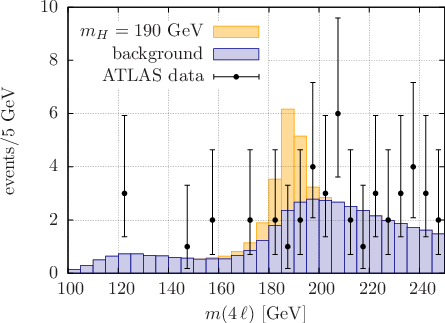

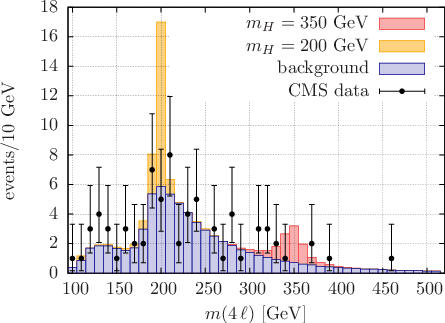
Due to the modifications of the Higgs sector that arise from Eq. (1) after electroweak symmetry breaking, both the partial decay width (i.e. the line shape) and the production cross section are modified. More precisely, the Unhiggs propagator reads [24]
| (2) |
where is the pole mass. The top-Yukawa coupling for follows from , where is the model’s cut-off scale (see Refs. [15, 24] for further details).
| (3a) | |||
| (3b) | |||
| where | |||
| (3c) | |||
The above modification of width stems from the pole contribution and its decay to SM particles. This should be contrasted to an additional imaginary part that the propagator Eq. (2) can pick up. Eq. (3b) gives an approximation for the pole contribution in terms of cross section times branching ratio. In the final analysis we use the full off-shell propagator including imaginary parts in Sec. IV, i.e. the one that arises from the conformal structure of the propagator and the one that arises from the decay of the state. Doing so, we recover the SM propagators, widths and cross sections upon taking the limit . This is also clear from Eq. (3a)-(3c), for we have .
The channel is potentially sensitive to both of these modifications in the heavy mass region , especially because the observed Higgs width is dominated by the physical one [3, 5]. For light Higgs particles the width is dominated by the detector resolution, also in the gold-plated decay mode (see e.g. [27]).
III Elements of the Analysis
Statistics
To formulate exclusion bounds on the Unhiggs model, we apply a binned log-likelihood ratio hypothesis test as formulated during the LEP2 era in the context of Higgs searches [28]. The test statistic is given by
| (4) |
where denotes the Poissonian likelihood, e.g.
| (5) |
where is the number of expected events at a given luminosity and is the number of actually observed events in the Unhiggs model. The generalization to binned histograms is straightforward.
The test statistic Eq. (4) is different from the profile likelihood which is employed by ATLAS and CMS [29] in its asymptotic behavior and in the treatment of uncertainties. Since the shape and systematic uncertainties are not publicly available, we neglect them throughout and take the distributions by ATLAS and CMS at face value.
| Signal hypothesis | 95% CL expected | 95% CL observed | ||||
|---|---|---|---|---|---|---|
| ATLAS | CLS | MC+CLS | ATLAS | CLS | MC+CLS | |
| 0.81 | 0.76 | 0.74 | 0.52 | 0.58 | 0.58 | |
| 0.79 | 0.76 | 0.76 | 0.57 | 0.56 | 0.57 | |
| Signal hypothesis | 95% CL expected | 95% CL observed | ||||
| CMS | CLS | MC+CLS | CMS | CLS | MC+CLS | |
| 0.50 | 0.49 | 0.50 | 0.62 | 0.52 | 0.60 | |
| 0.73 | 0.67 | 0.67 | 0.76 | 0.78 | 0.73 | |
It can be expected that the influence of marginalization over nuisance parameters [30] on the computed confidence level is not too important for this clean and well-reconstructible final state. Indeed, we compute 95% upper confidence levels using the CLs method [31] in Tab. 1, which are in good agreement with the results from ATLAS and CMS. This holds especially for large Higgs masses which we want to study in detail for the purpose of this work. Given this agreement with ATLAS and CMS, our implementation potentially reproduces the findings by ATLAS and CMS at the percent level, well inside the uncertainty bands for heavy Higgs bosons . For our CLS implementation shows deviations of for the experiments’ histograms as input. We interpret this deviation as the influence of systematics which plays an important role when the bosons are soft and off-shell. Since the resulting distributions’ shape uncertainties are not publicly known we cannot reproduce a quantitatively reliable agreement for within the limitations of our naive detector simulation (for details see below). This region requires the full experimental analysis flow, which is not available to us. Hence, we focus in the following on the heavy Higgses .


Event generation and MC Analysis
For the event generation we use a modified version of MadGraph v4 [32], which implements the Unhiggs model as described in Ref. [15]. The parton level events are subsequently showered with Pythia v6 [33]. To account for detector resolution effects we process the showered events with PGS [34]. In order to reliably reproduce the SM Higgs signal distributions that enter the hypothesis tests of ATLAS and CMS, we have performed a dedicated tune of PGS, leading to good agreement of the distribution at the percent level for heavy Higgs masses .
We adopt the cuts from the respective experimental analysis [3, 5]. Concretely this means selecting events with two same-flavor and opposite-sign lepton pairs with the following features required by each experiment:
ATLAS — The leptons are required to have
transverse momenta of at least , where two of
them need to pass from a further constraint of
GeV. They are reconstructed within the geometrical coverage of
and with a separation . The first reconstructed boson, , is required to
be on-shell by taking its invariant mass closest to the boson mass
within the range . The invariant mass of
the remaining lepton pair, denoted by , is required to be
. Where the threshold mass,
, depends on the reconstructed four-lepton
mass as denoted by the Tab. 2.
CMS — The leptons are required to have transverse
momenta of and being in the
pseudorapidity range of and ,
respectively. One of bosons is reconstructed by the pair
or within the mass range and with the transverse momenta for the lepton
pair or . The other boson
is selected by the remaining same flavor combination
and is denoted by . It is required that
with the additional constrain
. If more than one combination satisfies these
criteria for the one with the highest
leptons is chosen.
We compare the resulting confidence levels in Tab. 1, where “MC+CLS” denotes the hypothesis test with the background hypothesis extracted from the experiments and with the signal distributions generated by the described tool chain. In total we find very good agreement for high masses, so that our analysis set-up is sufficiently validated to confront the Unhiggs hypothesis with data
| 120 | 130 | 140 | 150 | 160 | 165 | 180 | 190 | 200 | |
| 15 | 20 | 25 | 30 | 30 | 35 | 40 | 50 | 60 |
IV Bounds on Unhiggs production from
We show the expected and observed 95% confidence level curves for the high mass values quoted in Tab. 1 in Fig. 2. Throughout, we plot exclusion limits in terms of as function of the Unhiggs scaling dimension , keeping fixed. dominantly depends on for this choice, and we discuss the influence of on the exclusion limits in detail later on. We also show the ATLAS CMS combination for in Fig. 3.
In Fig. 5 we show the dependence of on for a representative value of the Higgs mass. From this figure we see that a variation of in the signal hypothesis leaves our findings for largely unmodified unless we face a situation where the conformal symmetry breaking scale is close to the Unhiggs pole mass. If we consider the situation there is an additional contribution to the width [24], which eventually can yield . Consequently this region is already now excluded at the 95% confidence level by the combination, and the observed limits on are slightly larger than for , with a stronger dependence on .

The shape of the exclusion contours of Figs. 2 and 3 is representative for the entire considered mass range , while the quantitative details of the observed exclusion on is mostly driven by actually observed data around the signal hypothesis. Local deficits and excesses in the data do typically not change this situation, i.e. when we see a deficit in data this typically carries over to a larger-than-expected for fixed . The combination of both searches in regions where the data is consistent with the background allows to impose even stronger bounds on Unhiggs production, as can be seen from the comparison of Figs. 2 with 3.
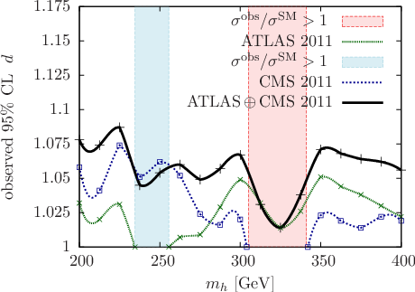
From Fig. 1 (and Refs. [3, 5]), it is clear that for some Higgs masses we observe excesses by the individual experiments. Since the Unhiggs model generically predicts smaller cross sections in for than encountered in the SM, we are therefore not able to put bounds on the Unhiggs model in these particular regions for the individual analyses. CMS and ATLAS, however, observe these excesses in different Higgs mass regions. This allows us to constrain the full considered Higgs mass range in the Unhiggs model from the combination of the ATLAS and CMS searches, yielding over the entire mass range . This is shown in Fig. 4, where we scan the observed 95% CL on over the mass range (again for ). The shaded areas represent Higgs mass regions where ATLAS and CMS cannot constrain the Unhiggs model individually. The combination of the two experiments amounts to a combined bound of . In the region where no bound can be imposed by the ATLAS experiment, the observed exclusion is , which results from a rather large upward fluctuation. This excess weakens the observed CMS exclusion in the combination, which holds also vice-versa for in a more pronounced way.
In total, the resulting SM bounds translate into only mild bounds on Unhiggs production, i.e. . Expecting in the Unhiggs scenario, these constraints are not strong enough to rule out the existence of the Unhiggs scenario. This, however, should be possible with the future increase of luminosity and center of mass energy.
V Summary and Conclusions
The LHC has tested Standard Model Higgs production at TeV center of mass energy with a luminosity of about 5 fb-1. Significant bounds on the SM Higgs could be established in 2011 by both ATLAS and CMS. The combination of both data sets allows to impose constraints over the range in the channel. We show that we can reproduce the experiments sensitivity to very good approximation, thus allowing us to understand the observed underproduction if a Higgs is realized in this particular mass range in terms of Unhiggs symmetry breaking. We find that the data only mildly constrains the Unhiggs scenario , with a very flat dependence of these results on the high scale conformal symmetry breaking scale as long as .
Acknowledgements.
We cordially thank the organizers of the Heidelberg New Physics Forum for a stimulating environment. C.E. and M.S. thank the University of California Davis for the kind hospitality during the time when parts of this work was done. C.E. also would like to thank Markus Schumacher for helpful discussions. C.E. acknowledges funding by the Durham Junior Research Fellowship scheme. D.G. acknowledges support by the International Max Planck Research School for Precision Tests. J.T. was supported by the Department of Energy under grant DE-FG02-91ER406746.References
- [1] ATLAS collaboration, ATLAS-CONF-2012-019. CMS collaboration, CMS-PAS-HIG-12-008.
- [2] ATLAS Collaboration, arXiv:1112.2577 [hep-ex], ATLAS-CONF-2011-162, ATLAS-CONF-2011-163.
- [3] ATLAS collaboration, ATLAS-CONF-2011-161.
- [4] CMS Collaboration, CMS-PAS-HIG-11-029, CMS-PAS-HIG-11-030, CMS-PAS-HIG-11-031, CMS-PAS-HIG-11-032.
- [5] CMS collaboration, CMS-PAS-HIG-11-025.
- [6] D. Carmi, A. Falkowski, E. Kuflik and T. Volansky, arXiv:1202.3144 [hep-ph]. A. Azatov, R. Contino and J. Galloway, arXiv:1202.3415 [hep-ph]. J. R. Espinosa, C. Grojean, M. Muhlleitner and M. Trott, arXiv:1202.3697 [hep-ph].
- [7] P. P. Giardino, K. Kannike, M. Raidal and A. Strumia, arXiv:1203.4254 [hep-ph]. J. Ellis and T. You, arXiv:1204.0464 [hep-ph].
- [8] B. A. Dobrescu, G. D. Kribs and A. Martin, arXiv:1112.2208 [hep-ph]. V. Ilisie and A. Pich, arXiv:1202.3420 [hep-ph].
- [9] C. Englert, J. Jaeckel, E. Re and M. Spannowsky, Phys. Rev. D 85 (2012) 035008. C. Cheung and Y. Nomura, arXiv:1112.3043 [hep-ph].
- [10] H. de Sandes and R. Rosenfeld, Phys. Rev. D 85, 053003 (2012). C. Englert, T. Plehn, M. Rauch, D. Zerwas and P. M. Zerwas, Phys. Lett. B 707 (2012) 512.
- [11] J. M. Campbell, W. T. Giele and C. Williams, arXiv:1204.4424 [hep-ph].
- [12] I. Low, P. Schwaller, G. Shaughnessy and C. E. M. Wagner, Phys. Rev. D 85 (2012) 015009. S. Goria, G. Passarino and D. Rosco, arXiv:1112.5517 [hep-ph].
- [13] S. Y. Choi, D. J. Miller, M. M. Muhlleitner and P. M. Zerwas, Phys. Lett. B 553, 61 (2003). C. P. Buszello, I. Fleck, P. Marquard and J. J. van der Bij, Eur. Phys. J. C 32 (2004) 209.
- [14] C. Hackstein and M. Spannowsky, Phys. Rev. D 82, 113012 (2010). C. Englert, C. Hackstein and M. Spannowsky, Phys. Rev. D 82 (2010) 114024.
- [15] C. Englert, M. Spannowsky, D. Stancato and J. Terning, arXiv:1203.0312 [hep-ph].
- [16] G. ’t Hooft, Nucl. Phys. B 72 (1974) 461.
- [17] J. M. Maldacena, Adv. Theor. Math. Phys. 2, 231 (1998) [Int. J. Theor. Phys. 38, 1113 (1999)] [hep-th/9711200]. S. S. Gubser, I. R. Klebanov and A. M. Polyakov, Phys. Lett. B 428, 105 (1998) [hep-th/9802109]. E. Witten, Adv. Theor. Math. Phys. 2, 253 (1998) [hep-th/9802150].
- [18] N. Arkani-Hamed, M. Porrati and L. Randall, JHEP 0108 (2001) 017. R. Rattazzi and A. Zaffaroni, JHEP 0104, 021 (2001). M. Perez-Victoria, JHEP 0105, 064 (2001). C. Csaki, M. Reece and J. Terning, JHEP 0905 (2009) 067.
- [19] L. Randall and R. Sundrum, Phys. Rev. Lett. 83 (1999) 3370. L. Randall and R. Sundrum, Phys. Rev. Lett. 83 (1999) 4690.
- [20] K. Agashe, A. Belyaev, T. Krupovnickas, G. Perez and J. Virzi, Phys. Rev. D 77 (2008) 015003. A. L. Fitzpatrick, J. Kaplan, L. Randall and L. -T. Wang, JHEP 0709 (2007) 013. B. Lillie, J. Shu and T. M. P. Tait, Phys. Rev. D 76 (2007) 115016. K. Agashe, H. Davoudiasl, S. Gopalakrishna, T. Han, G. -Y. Huang, G. Perez, Z. -G. Si and A. Soni, Phys. Rev. D 76 (2007) 115015. B. Lillie, L. Randall and L. -T. Wang, JHEP 0709 (2007) 074. C. Englert, B. Jager, M. Worek and D. Zeppenfeld, Phys. Rev. D 80 (2009) 035027.
- [21] R. Contino, Y. Nomura and A. Pomarol, Nucl. Phys. B 671 (2003) 148. R. Contino, T. Kramer, M. Son and R. Sundrum, JHEP 0705, 074 (2007). R. Contino, D. Marzocca, D. Pappadopulo and R. Rattazzi, JHEP 1110 (2011) 081.
- [22] G. Cacciapaglia, G. Marandella and J. Terning, JHEP 0801 (2008) 070. A. Falkowski and M. Perez-Victoria, JHEP 0812, 107 (2008). G. Cacciapaglia, G. Marandella and J. Terning, JHEP 0902, 049 (2009). A. Falkowski, M. Perez-Victoria, Phys. Rev. D79, 035005 (2009).
- [23] H. Georgi, Phys. Rev. Lett. 98 (2007) 221601. H. Georgi, Phys. Lett. B 650, 275 (2007).
- [24] D. Stancato and J. Terning, JHEP 0911, 101 (2009).
- [25] A. Falkowski, M. Perez-Victoria, JHEP 0912, 061 (2009).
- [26] T. Han, D. Krohn, L. T. Wang and W. Zhu, JHEP 1003 (2010) 082.
- [27] G. Aad et al. [ATLAS Collaboration], JINST 3 (2008) S08003, G. L. Bayatian et al. [CMS Collaboration], J. Phys. G 34 (2007) 995.
- [28] R. Barate et al. [LEP Working Group for Higgs boson searches], Phys. Lett. B 565 (2003) 61. P. Bock et al. [ ALEPH and DELPHI and L3 and OPAL Collaborations ], CERN-EP/98-046.
- [29] G. Cowan, K. Cranmer, E. Gross and O. Vitells, Eur. Phys. J. C 71, 1554 (2011).
- [30] T. Junk, Nucl. Instrum. Meth. A 434 (1999) 435. T. Junk, CDF Note 8128 [cdf/doc/statistics/public/8128]. T. Junk, CDF Note 7904 [cdf/doc/statistics/public/7904]. H. Hu and J. Nielsen, in 1st Workshop on Confidence Limits’, CERN 2000-005 (2000).
- [31] A. L. Read, CERN-OPEN-2000-205. A. L. Read, J. Phys. G G28 (2002) 2693-2704.
- [32] J. Alwall, P. Demin, S. de Visscher, R. Frederix, M. Herquet, F. Maltoni, T. Plehn and D. L. Rainwater et al., JHEP 0709 (2007) 028.
- [33] T. Sjostrand, S. Mrenna and P. Z. Skands, JHEP 0605, 026 (2006).
- [34] J. Conway et al., http://physics.ucdavis.edu/~conway/research/software/pgs/pgs4-general.htm.