Refining inflation using non-canonical scalars
Abstract
This paper revisits the Inflationary scenario within the framework of scalar field models possessing a non-canonical kinetic term. We obtain closed form solutions for all essential quantities associated with chaotic inflation including slow roll parameters, scalar and tensor power spectra, spectral indices, the tensor-to-scalar ratio, etc. We also examine the Hamilton-Jacobi equation and demonstrate the existence of an inflationary attractor. Our results highlight the fact that non-canonical scalars can significantly improve the viability of inflationary models. They accomplish this by decreasing the tensor-to-scalar ratio while simultaneously increasing the value of the scalar spectral index, thereby redeeming models which are incompatible with the cosmic microwave background (CMB) in their canonical version. For instance, the non-canonical version of the chaotic inflationary potential, , is found to agree with observations for values of as large as unity ! The exponential potential can also provide a reasonable fit to CMB observations. A central result of this paper is that steep potentials (such as ) usually associated with dark energy, can drive inflation in the non-canonical setting. Interestingly, non-canonical scalars violate the consistency relation , which emerges as a smoking gun test for this class of models.
Keywords
Inflation1 Introduction
Since its inception over three decades ago [1] the inflationary paradigm has moved to the center stage of modern cosmology. The amelioration of the horizon and flatness problems – a generic feature of the inflationary mechanism – was spectacularly confirmed by cosmic microwave background (CMB) experiments of the 1990’s. The other important prediction of inflation – that of a near scale invariant perturbation spectral index [2] has also found convincing support in recent CMB measurements [3]. Yet other important consequences of the inflationary scenario, such as the presence of a relic gravity wave background and possible departures from non-Gaussianity, will be tested by current and future probes of the CMB including the PLANCK surveyor, QUaD, BICEP2, SPIDER, CMBpol, etc.
Despite its remarkable successes the inflationary scenario has, on occasion, been described as a paradigm in search of a model [4]. While models of inflation abound in the literature [5, 15, 16, 17, 18, 19, 20, 21], the simplest inflationary potential described by the quartic self-interaction runs into trouble with the CMB. The problems with this potential are two fold: (i) its prediction of tensor fluctuations (gravity waves) are too large and appear to conflict with current bounds on the tensor-to-scalar ratio. (ii) The value of the dimensionless constant, , inferred from CMB observations is anomalously small, , much smaller for instance than the coupling constant of the Higgs boson [22] .
Perhaps the simplest generalization of the inflationary scenario involves extending the inflationary Lagrangian to accommodate non-canonical kinetic terms. It is well known that the equations of motion remain second order, which is an attractive feature of this class of models. Furthermore, as we demonstrate in this paper, the slow-roll conditions become easier to satisfy with the result that the tensor-to-scalar ratio drops considerably (relative to the canonical case). These properties of non-canonical scalars have wide reaching ramifications:
- •
Chaotic inflation with the potential satisfies current CMB constraints, and large values of can be accommodated by the data making this model physically appealing. (By comparison an astonishingly small value is demanded of canonical inflation by observations.)
- •
The exponential potential, which is in tension with observations in the canonical case, also comes into favor since its tensor-to-scalar ratio can lie within the observationally acceptable range. As a result the potential which allows an exponential-type potential to oscillate becomes an interesting inflationary contender.
- •
Steep potentials such as , which are commonly associated with dark energy in the canonical case, can source inflation for non-canonical fields.
- •
As pointed out in [24], inflation sourced by non-canonical scalars violates the consistency relation , which emerges as a smoking gun for this class of models.
One might add that the purpose of the present paper is not to add yet another theoretical construct to the already burgeoning inflationary-model inventory. Instead, building on earlier work [23, 24], we present a new dynamical framework flexible enough to accommodate within its fold different classes of inflationary models including large field models such as chaotic inflation, as well as small field models. Indeed the formulae presented in §2 are sufficiently general to allow the reader to translate a canonical inflationary model into its non-canonical counterpart, obtaining in the process important observational quantities including power spectra, the spectral indices , , the tensor-to-scalar ratio, , etc.
This paper is organized as follows. The field equations are set up in section 2 which also contains a discussion of the slow roll parameters and the Hamilton-Jacobi equation for non-canonical scalars. Inflationary models and CMB constraints on model parameters are the focus of section 3. Non-canonical scalar fields have difficulty in oscillating which could make reheating problematic in this scenario. This important drawback is both noticed and corrected in section 4. Our main conclusions are drawn in section 5.
2 Cosmological dynamics
2.1 Field equations
Consider a scalar field which couples minimally to gravity and for which the action has the following general form
| (1) |
where the Lagrangian density can be an arbitrary function of the field and the kinetic term
| (2) |
Numerous functional forms of have been considered in the literature, see for instance Refs.[23, 24, 25, 26, 27, 28, 29, 30, 31, 32, 33, 34, 35]. Varying the action (1) with respect to leads to the equation of motion
| (3) |
In a spatially flat Friedmann-Robertson-Walker (FRW) universe
| (4) |
the field is a function only of time i.e., , hence the equation of motion (3) reduces to
| (5) |
The energy-momentum tensor associated with the scalar field is
| (6) |
In a spatially flat FRW universe
| (7) |
where the energy density, , and pressure, , are given by
| (8) | |||||
| (9) |
and . The evolution of the scale factor is governed by the Friedmann equations:
| (10) | |||||
| (11) |
where satisfies the conservation equation
| (12) |
Note that the equation of motion for in (5) also follows from the conservation equation (12).
Our non-canonical scalar field model has the Lagrangian density [28, 29]
| (13) |
where has dimensions of mass while is dimensionless. When the Lagrangian (13) reduces to the usual canonical scalar field Lagrangian . Throughout this paper we shall assume and work with natural units, viz. .
The energy density and pressure are obtained by substituting (13) into (8) and (9), we find
| (14) |
which reduces to the canonical form , when . Consequently the two Friedmann equations (10) and (11) become [29, 30]
| (15) | |||||
| (16) |
and the following scalar field equation of motion follows from eq.(5)
| (17) |
which reduces to when .
2.2 Slow roll parameters
The two slow roll parameters are defined according to convention as
| (18) |
Since , it follows that the universe accelerates (inflates) when . Substituting for and from (14) into
| (19) |
it is easy to show that the FRW equation (15) reduces to
| (20) |
As concerns the second slow roll parameter, one finds
| (21) |
and substituting (21) into (17) we obtain
| (22) |
It is easy to show that the slow roll conditions , , imply the following relations between the slow roll parameters and the inflaton potential:
| (23) |
| (24) |
where the parameter
| (25) |
plays a key role in inflationary and quintessence model building. For the canonical scalar field with equations (23), (24) converge to the standard ‘canonical’ expressions
| (26) | |||||
| (27) |
Note that the slow roll assumption leads to
| (28) |
where when ; when This equation shall prove useful when we derive an expression for the number of inflationary e-folds in the next section.
Equation (23) can be written in a more suggestive manner as
| (29) |
where corresponds to the canonical value of in (26). Since it follows that the first term in the right hand side of (29) is smaller than unity. We therefore find that the slow roll parameter in non-canonical models can become smaller than its canonical counterpart, ie , when . We shall return to this issue in section 3, where we show that sub-Planckian values of provide better agreement with observations for a large family of inflationary models. Another aspect of (29) is that inflation can be sourced by steep potentials in non-canonical models, which is discussed next.
2.3 Inflation with steep potentials
Equation (29) with implies the inequality
| (30) |
which allows inflation to be sourced by steep potentials when . Note that the possibility of sourcing inflation using steep potentials has earlier been discussed in the braneworld context in [8].
Indeed, equation (30) bears a close similarity to the relationship between slow roll parameters in an RSII braneworld cosmology. The latter is described by the equations [6, 7, 8]
| (31) |
where and is the three dimensional brane tension. As noted by a number of authors [8, 9, 10] the motion of a canonical scalar field propagating on the brane
| (32) |
is heavily damped due to the increased value of the term when in (31). This causes the field to roll slower than it would in an FRW cosmology which is reflected in the value of the slow roll parameter on the brane
| (33) |
where is the canonical value in an FRW universe, namely (27). Comparing (30) & (33) we find that the parameter in non-canonical models plays a role similar to that of the brane tension in braneworld cosmology. In the braneworld case when in (33), while for non-canonical scalars when in (29) or (30).
It is well known that inflation can be driven by steep potentials in braneworld models [8, 9, 10] and this intriguing possibility can be realized for non-canonical scalars as well. We illustrate this for two potentials commonly associated with dark energy in the canonical case: (i) the inverse power law potential [12] and (ii) the exponential potential [13] .
- 1.
For the inverse power law potential
(34) one finds
(35) so that for the value of does not depend upon ! In this case
(36) and it is easy to see that for and . We therefore find that the inverse power law potential, which is associated with dark energy in its canonical version, can source inflation for non-canonical fields ! From (35) we also find that
(37) when and . Therefore we arrive at the following interesting result: in a non-canonical setting it may be possible for the inverse power law potential (34) to source small field inflation provided and .
- 2.
For the exponential potential
(38) one finds
(39) which rules out canonical inflation for such ultra-steep potentials.
We therefore conclude that non-canonical models bring more diversity into inflationary model building by permitting inflation to be sourced by flat as well as steep potentials.
As in the braneworld case [9, 10, 11], the possibility of sourcing inflation using steep potentials might allow one to construct models of Quintessential Inflation [14] based on non-canonical scalars. We shall return to this possibility in a future work.
We end this section with a cautionary note. It is formally not very meaningful to claim that a potential is steep without reference to the kinetic term. For instance, one can convert a flat potential into a steep one using a field redefinition, but then one also changes the form of the kinetic term, as illustrated in the appendix. For this reason one should exercise some care when comparing models with different kinetic terms. In our discussion above, results for the braneworld model were based on the behavior of a canonical scalar field propagating on the brane, whereas our own model is based on the non-canonical Lagrangian (13). (The propagation of non-canonical scalar fields on the brane has, to the best of our knowledge, not yet been studied.)
2.4 Hamilton-Jacobi equation and the Inflationary Attractor
The slow roll parameters on their own do not necessarily encapsulate the full dynamical picture of inflation. The fact that the equations of motion of the inflaton are of second order makes it possible to change initial conditions (value of ) so as to arrive at a different set of observational predictions for inflation [15]. Clearly in order for inflation to be a robust theory its predictions should not be unduly sensitive to initial conditions. In other words, it would be desirable if the difference between nearby trajectories were to rapidly decay during inflation. That this is indeed the case was shown in several early papers which demonstrated the existence of an inflationary attractor solution [36].
The presence of the inflationary attractor is easiest to demonstrate using the Hamilton-Jacobi formalism [37], and we shall adopt this method for our present analysis. The idea behind the Hamilton-Jacobi formalism is to rewrite the Friedmann equation (15) as an evolution equation for . For the non-canonical case this is done by noting that
| (41) |
substituting for and from (14)) and rearranging, gives
| (42) |
where
In the above equation overprime denotes derivative with respect to . It is evident from the above equation that the sign of and are opposite to each other. The above equation implies
| (43) |
on substituting this equation in the Friedmann equation (15), gives
| (44) |
where
| (45) |
Equation (44) is Hamilton-Jacobi equation corresponding to the non-canonical Lagrangian (13). For , and (44) reduces to the standard Hamilton-Jacobi equation for the canonical scalar field, namely
| (46) |
The Hamilton-Jacobi equation (44) allows us to determine for a given . Conversely, one can also reconstruct the potential if have prior knowledge of . It is important to note that, for any given , each phase-space trajectory can be mapped to a corresponding . This follows from the Friedmann equation (15). Therefore, for a given potential , let and be two nearby phase-space trajectories corresponding to the homogeneous solutions and , respectively. Substituting these into the Hamilton-Jacobi equation (44) and linearizing gives
| (47) |
which is easily solved to give
| (48) |
here is the value of the perturbed Hubble parameter corresponding to some initial . Since, is number of efolds counted from the end of inflation
| (49) |
substituting for from (42) into the above equation gives
| (50) |
Finally, using (45), (48) & (50), we find the following simple expression describing the decay of perturbations
| (51) |
and signifying an exponentially rapid approach to the inflationary attractor solution.
Remarkably our final expression (51)
does not depend on either or , the two
free parameters which characterize our model (13). Since
the rate at which a nearby trajectory converges to is
independent of and we conclude
that homogeneous perturbations in non-canonical inflationary models decay in
precisely the same manner as they do for canonical scalars [37].
Evolution of slow roll parameter
The above argument shows that two nearby phase-space trajectories, whether inflationary or not, converge, thereby ascertaining the dynamical stability of the system. However, as far as inflation is concerned, it is important to examine whether the inflationary trajectory is an attractor. To address this issue, we investigate how the slow roll parameter defined in Eq.(18) evolves as the scalar field rolls down the potential.
From the definition of the slow roll parameter (18) and using (15) and (16), we have
| (52) |
Therefore, for , the allowed range of is
| (53) |
where the lower limit corresponds to the equation of state parameter , whereas the upper bound corresponds to .
Using Eqs.(14) and (52), the potential can be expressed as
Therefore,
| (54) |
Since , it follows that and therefore, Eq.(42) can be re-expressed as
| (55) |
where when and when The sign of ensures that scalar field rolls down the potential. Substituting Eq.(55) in Eq.(54) and on rearranging, we arrive at the following equation of motion for :
| (56) |
where is the slow roll parameter defined in terms of the potential in (23).
Note that equation (56) is exact and the slow roll approximation has not been used in its derivation. Using (56), one can investigate how the slow roll parameter evolves as the scalar field rolls down its potential and thereby ascertain whether the slow roll inflationary trajectory () is an attractor. Let us first consider the canonical scalar field case which corresponds to setting in (56) so that this equation reduces to
| (57) |
where is given by (26) for canonical inflation. Since always lies between and and in an expanding universe, the sign of (at a given value of ) is determined by the last term in the left hand side of (57). In other words the sign of depends upon the value of , which quantifies the departure of from its slow roll value .
-
Eqn (57) suggests that if, for a given phase-space value one finds , then so that is driven towards .
-
On the other hand if , then , so in this case also is driven towards .
We therefore find that is always driven towards so that the slow roll trajectory () is an attractor.
It is easy to see that similar results follow from (56) for . The slow roll inflationary trajectory corresponds to and . If, for a given value of , , and the value of is such that:
-
, then it follows from (56) that and is driven towards .
-
, then is implied by (56), so that once more is driven towards .
We therefore conclude that for any potential possessing a regime satisfying , the slow roll inflationary trajectory is indeed an attractor.
Consider next an inflationary potential for which the slow roll parameter in (56) becomes very small, ie . The worst case scenario for inflation is clearly when the kinetic term is very large so that and . It is easy to see that in this case (56) can be approximated as
| (58) |
which has the solution
| (59) |
where is a constant of integration. From (59) it follows that as the universe expands () the slow roll parameter decays as and soon approaches , signalling the advent of slow-roll and .
2.5 Scalar and tensor power spectra
Linearized scalar and tensor perturbations within the spatially flat FRW context are described by the line element [38, 39, 40]
where , , and describe the scalar degree of metric perturbations while are tensor perturbations. We consider only scalar and tensor perturbations since it is well known that scalar fields do not lead to vector perturbations. The curvature perturbation on the uniform field slicing is defined as a gauge invariant combination of the metric perturbation and scalar field perturbation , namely
| (60) |
From the Linearized Einstein’s equation and from the equation governing the evolution of perturbations in the scalar field, it turns out that
| (61) |
where overprime denotes derivative with respect to conformal time, ; is the square of the effective speed of sound of the scalar field perturbation [24]
| (62) |
and is given by
| (63) |
Rewriting (61) in terms of the Mukhanov-Sasaki variable , one gets
| (64) |
The corresponding equation governing the tensor perturbations is
| (65) |
where and is the amplitude of the tensor perturbation.
The power spectrum of scalar curvature perturbations is defined as
| (66) |
while the tensor power spectrum is
| (67) |
Following [24], the expression for scalar and tensor power spectrum in the slow roll limit turns out to be
| (68) |
and
| (69) |
For the Lagrangian density (13), the scalar power spectrum in the slow roll regime is determined from (68) to be
| (70) |
The speed of sound determined from (13) and (62) is
| (71) |
We therefore find that the sound speed is a constant. The focus of this paper will be on for which (ie since we work with units ).
3 Inflationary models
3.1 Chaotic inflation
Chaotic inflation is usually associated with power law potentials
| (72) |
In what follows we shall obtain an expression for , with being the number of inflationary e-folds to the end of inflation. Inflation ends when slow-roll parameters grow and approach the value of unity. Substituting in (23) we obtain the following expression for the value of the scalar field when inflation ends
| (73) |
where
| (74) |
The number of e-folds to the end of inflation is
| (75) |
Substituting for from (28) and for from (73) we obtain the following simple expression
| (76) |
where
| (77) |
which reduces to the standard result
| (78) |
We now use the results of the preceding section to determine spectral indices for scalar and tensor perturbations. Substituting (72) in (70) we find
| (79) |
where was defined in (74) and the amplitude is given by
| (80) |
The scalar spectral index is defined as
| (81) |
Since constant during slow roll inflation and is constant for our model, it turns out that at sound horizon exit ()
| (82) |
where is the number of e-folds counted from the end of inflation. Therefore, from (79), (81), (82) we have
| (83) |
Substituting for from (76) into the above equation gives the elegant and simple result
| (84) |
with defined in (72) and defined in (74). The running of the spectral index is given by
| (85) |
For , eqn (84) reduces to the standard result for large field inflationary models with a canonical kinetic term, namely
| (86) |
Several points need to be noted here:
- •
- •
- •
Generically, for in , the value of asymptotically approaches the constant value
(89) Indeed, from the left panel of figure 1 we see that as increases the value of for the potential with approaches the value of for the potential with the lower value of .


Turning now to the tensor power spectrum and substituting in (69) we get
| (90) |
An analytical form for the tensor spectral index
| (91) |
can be obtained by substituting from (76) into (90) and using (82), it follows that
| (92) |
where was defined in (74).
We now proceed to obtain the tensor-to-scalar ratio
| (93) |
When evaluating it is important to keep in mind that the expression (79) for the scalar power spectrum is evaluated at sound horizon exit () while the corresponding expression (90) for the tensor power spectrum is evaluated at horizon exit (). However, since constant during slow roll, and the speed of sound does not depend upon time, the value of the field at sound horizon exit is approximately the same as at horizon exit [24]. Therefore, substituting (79) and (90) in (93) and using from Eq.(76) we finally get
| (94) |
which is the standard value for canonical scalars.
The prefactor in (94) informs us that the value of decreases as is increased. In other words, non-canonical models with generically give rise to a lower tensor-to-scalar ratio than canonical models, which is one of the central results of this paper and is illustrated in figure 1. A lower value of helps in making the potential come into agreement with CMB data, as shown later in this section. Indeed, the right panel of fig. 1 illustrates that, for , the value of for the potential with overlaps with the value of for the potential with .
Using (94) and (92) one finds the following consistency relation for slow roll inflation with a non-canonical scalar field [24]
| (95) |
Note that the presence of the sound speed in (95) causes the consistency relation to differ from the canonical case for which . Substituting for from (71) we find
| (96) |
Since we find that the value of for non-canonical models is generically smaller than that for canonical models with identical values of .
For comparison note that a prominent example of a non-canonical scalar is provided by the tachyon model [25, 26, 27] for which and the speed of sound and equation of state are related through . Since during slow roll, it follows that for this class of models. Consequently, the consistency relation for slow roll inflation in tachyon models is the same as that for canonical scalar fields, namely . This is certainly not the case for our model (13) since even in the slow roll regime an appropriate choice of the free parameter can modify the speed of sound and hence the consistency relation (95). We therefore conclude that the consistency relation can help differentiate between our non-canonical model (13) and standard (slow roll) inflationary models as well as tachyon models. Eqn. (96) therefore emerges as a smoking gun test for the inflationary models examined in this paper [24].
CMB normalization
The scalar power spectrum (79) requires to be normalized using CMB observations. This can be done in a straightforward manner by noting that , where is the pivot scale [41]. Substituting the solution from (76) into the expression (79) and rearranging, we get for the potential
| (97) |
where was defined in (74) and denotes the number of e-folds from the end of inflation to the pivot scale. The above equation allows one to determine the value of the mass in and that of in .
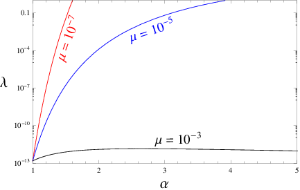
- •
- •


Our results for are illustrated in figure 2 which contains the following interesting information. For the value of grows as increases. Indeed the growth of becomes quite spectacular for smaller values of . For instance when , grows by over 10 orders of magnitude from its canonical value of for , to for . Furthermore figure 1 informs us that for the tensor-to-scalar ratio in this model is , which is in good agreement with observations – see fig. 3. One might also like to note that smaller values of are more physically appealing since they correspond to sub-Planckian mass scales, with GeV being the energy scale of Inflation. [ and have been defined in (13) for our model.] We therefore come to the conclusion that Inflation, which runs into CMB trouble in the canonical case, reverts back into favor when viewed within a non-canonical setting. (Similar results have been recently obtained in [42] for an inflationary model with a field derivative coupling to gravity; see also [43].)
3.2 The exponential potential
Another important example of a ‘large field’ potential is the exponential
| (102) |
A spatially flat universe dominated by a canonical scalar field with this potential expands as a power law [44]. It is easy to see that in this case the slow roll parameters in (18) & (23) are constants , making a natural exit from inflation impossible. Remarkably this is not the case for non-canonical models for which the slow roll parameter in (23) acquires the form
| (103) |
which reduces to for . Clearly for the value of can be extremely small if . Thus the slow roll parameter evolves from initially, to as rolls down its potential and increases 11 1 As mentioned earlier, we only consider the case where the parameter . This will ensure that the speed of sound is less than the speed of light. It is only when evolves from and crosses when scalar field rolls down the potential. However, when , the slow roll parameter in fact decreases as the scalar field rolls down the potential which makes exit from inflation even more difficult to attain.. Inflation based on the exponential potential with a non-canonical scalar therefore has a graceful exit !
From (28) and (103) one can show that in the slow roll regime
| (104) |
Differentiating (103) with respect to and using the above equation, we arrive at the following equation of motion for :
| (105) |
which can be solved to give
| (106) |
Equation (105) ensures that when , is identically constant and to be consistent with the standard result, its value should be . However, from the solution (106), it turns out that for , the slow roll parameter is independent of the value of and astonishingly the solution does not converge to the standard result (viz. ) when is set to unity. As we shall see shortly, in addition to neither nor depend on , and the reason for this puzzling behavior will be explained at the end of this section.

For the exponential potential, the expression for scalar power spectrum (70) reduces to
| (107) |
where the amplitude is given by
| (108) |
Using Eqs.(82) and (104), the scalar spectral index (81) for the exponential potential turns out to be
| (109) |
Substituting from (106) we get
| (110) |
Similarly, using Eqs.(67), (93), (103),(107) and (106), we get the following result for the tensor to scalar ratio
| (111) |
Our results for and are shown together with CMB constraints in figure 4. We find that for the exponential potential can be accommodated by observations.
As mentioned earlier, the expressions for and do not depend on the value of in (102) when . The reason for this stems from the fact that under the transformation , the Lagrangian (13) with an exponential potential becomes
| (112) |
where
| (113) |
We therefore find that it is possible to absorb the parameter into a redefinition of the mass without altering the structure of the kinetic term in the Lagrangian. (This is possible only for .) As the mass in the kinetic term does not explicitly influence the value of either or , it is but natural to expect neither of these quantities to dependent on the parameter in the potential (102).
4 Scalar field oscillations and the equation of state
Non-canonical scalar field models have difficulty in oscillating which could make reheating problematic in this scenario. This can easily be seen from the following argument. Conventionally, after inflation has ended, the inflaton field commences to oscillate about the minimum of its potential. During any given oscillation the field amplitude is bounded by points where the field trajectory reverses, so that . This usually occurs in regions where and . Such oscillations are could be problematic within the non-canonical framework since, according to the field equation (17), when and .
To resolve this issue, one needs to regularize the field equation so that the value of remains finite even when . With this in mind, we propose a modified version of our model replacing (13) by the following ‘regularized’ Lagrangian:
| (114) |
where is a dimensionless parameter. The above prescription is tantamount to the addition of a canonical kinetic term to the original Lagrangian in (13). From (114) one finds that
- •
In the limit when , the Lagrangian converges to defined in (13). Therefore, all the results obtained in the preceding sections also follow from in the limit when .
- •
When or when , the Lagrangian reduces to the standard Lagrangian for the canonical scalar field.
For the modified model (114), the equation governing the evolution of the scalar field is given by
| (115) |
The above equation reduces to (17) when . When or , the equation (115) becomes the usual Klein-Gordon equation for the canonical scalar field. In the limit when , the above equation can be approximated as
| (116) |
where is an infinitesimally small correction factor when . Equation (116) is the regularized version of the field equation (17) in which acts as a small correction factor which ensures that remains finite even when and . With this correction in place the scalar field can oscillate about the minimum of its potential once inflation ends.
We now derive an expression for the average of the equation of state parameter for the oscillating scalar field. For the model (114), the energy density and pressure are given by
| (117) |
Since , in the limit when one finds
| (118) |
where denotes the average over one oscillation cycle. As in the case of standard canonical inflation, we shall assume that the time scale of oscillation is much smaller than the time scale of expansion of the universe. In this limit, the time variation of during any one cycle is sufficiently small to permit the approximation , where is the maximum value of the field during a given cycle. Using Eq.(117) and the fact that , we find that in the limit
| (119) |
From Eqs.(118) and (119) it is straight forward to show that
| (120) |
It can be verified that the above expression reduces to the standard result for the canonical scalar field when the parameter is set to unity (see Eq.(11) of Ref.[45]).
For chaotic potentials of the form , one integrates (120) to determine
| (121) |
The following points in relation to (121) deserve special mention:
- 1.
For the above expression reduces to the standard result [45]:
(122) - 2.
For , and therefore the oscillating scalar field cosmologically mimics the dynamics of the pressureless matter (dust). For example, when , a scalar field oscillating about the minimum of a potential would effectively behave as dust, in stark contrast to the canonical case for which .
- 3.
- 4.
For , it follows from equation (123) that
(125) From the above equation it is clear that asymptotically when , . Therefore, for the oscillating scalar field to behave as a fluid with , the value of in the potential must be less than .
These features have been illustrated in Fig. 5.

The fact that our new formalism (114) permits non-canonical fields to oscillate, and the observation that for sufficiently large values of the exponential potential provides a plausible inflationary model, allows us to introduce the following inflationary potential
| (126) |
which had been suggested as a dark matter candidate in [46]. The potential (126) has the following asymptotic forms:
| (127) |
A non-canonical scalar field rolling down such a potential could initially give rise to inflation following the discussion in section 3.2. Later, when dropped to sufficiently small values the scalar field would oscillate, and its mean equation of state would be given by
| (128) |
implying for . Whether the standard reheating mechanism will work for such a potential remains an interesting open question.
5 Conclusions
Focussing on a particular class of non-canonical scalar field models, namely those based on the Lagrangian density (13), we have shown that such models provide an attractive setting in which to re-examine Inflation. Our non-canonical inflationary models generically possess a lower tensor-to-scalar ratio and, in some cases, also a higher value of the scalar spectral index as compared to their canonical counterparts. This leads to a better agreement with observations as illustrated by the potential which agrees with CMB data for values of as large as .
It is well known that the exponential potential, in the canonical case, gives rise to (eternal) power law inflation and therefore faces a serious ‘graceful exit’ problem. On examining its non-canonical counterpart we find that inflation for this potential is no longer eternal, and, like its sister potentials , the exponential exits the slow-roll regime and therefore does not face a graceful exit problem. Furthermore it turns out that the tensor-to-scalar ratio is smaller for the exponential than in the canonical case, leading to better agreement with observations.
We also find that, under certain conditions, the inverse power law potential and other steep potentials commonly associated with dark energy in the canonical case, can source inflation for non-canonical fields. This considerably broadens the class of potentials used for inflationary model building and could open up the possibility of constructing models of Quintessential-Inflation in the non-canonical setting. Whether steep potential will satisfy the stringent constraints on imposed by the CMB will form the subject of a future investigation.
Our study in section 4 has shown that non-canonical scalar fields have difficulty in oscillating. Since oscillations are an integral part of preheating scenario’s [18, 47, 48, 49] this difficulty could prove calamitous for inflationary models in the non-canonical setting. The addition of a canonical kinetic term resolves this issue as shown in section 4; also see [50].
To summarize, we have shown in the context of large field models, that inflation becomes easier to realize if one generalizes the scalar field Lagrangian to accommodate non-canonical scalars. (Similar results have been obtained for an affiliated class of models in [51].) Our treatment in this paper has been quite general and should be straightforward to generalize to small field inflationary models. Whether the positive features of large field models carry over to small field ones remains an open question requiring further examination. Non-canonical scalar fields violate the consistency relation , which emerges as a smoking gun test for this class of models. Another test could be the extent of non-Gaussianity in the perturbation spectrum which we shall revert to in a future work.
After this paper was completed we became aware of [52] containing results which partially overlapped with ours.
Acknowledgements.
We acknowledge useful discussions with Charles Jose, Minu Joy, Jayanti Prasad, L. Sriramkumar and Tarun Souradeep. We also benefitted from comments made by the referee which led to an improvement in the manuscript.Appendix A Field redefinitions
Under the field redefinition
| (129) |
where is a constant, the Lagrangian (13) with a power law potential becomes
| (130) |
where
and
We therefore find that the structure of the Lagrangian (2.13) with a power law potential is invariant under the field redefinition . Only the parameters and are influenced by such a redefinition. It is evident from Eqs.(84) and (94) that the values of the scalar spectral index and the tensor to scalar ratio are independent of both and . This implies that such observables are immune to the field redefinition in the chaotic inflationary model based on (2.13). (This statement might even be true for generic field redefinitions.)
Field redefinitions of the form (129) do not affect the form of the potential. However, with suitable transformations such as , it is possible to convert a flat potential into a ‘steep’ one but with a different kinetic term in the Lagrangian. We illustrate this for the non-canonical scalar field model (13) with a quadratic potential
| (131) |
It is straightforward to show that under the transformation
| (132) |
the Lagrangian (131) becomes
| (133) |
where
| (134) |
Therefore, although the potential in (133) is steep for , the structure of the kinetic term is different from that in (13). It is therefore important to note that the steep potentials discussed in this paper are considered in the context of a given form of the kinetic term, namely the one described by (13).
References
- (1)
A. A. Starobinsky, A new type of isotropic cosmological models without singularity, Phys. Lett. B 91, 99 (1980);
A. H. Guth, Inflationary universe: A possible solution to the horizon and flatness problems Phys. Rev. D 23, 347 (1981);
A. D. Linde, A new inflationary universe scenario: A possible solution of the horizon, flatness, homogeneity, isotropy and primordial monopole problems, Phys. Lett. B 108, 389 (1982);
A. Albrecht and P. J. Steinhardt, Cosmology for Grand Unified Theories with Radiatively Induced Symmetry Breaking, Phys. Rev. Lett. 48, 1220 (1982);
A. D. Linde, Phys. Lett. B, Chaotic inflation 129, 177 (1983). - (2)
V. F. Mukhanov and G. V. Chibisov, Quantum fluctuations and a nonsingular universe JETP Lett. 33, 532 (1981);
S. W. Hawking, The development of irregularities in a single bubble inflationary universe, Phys. Lett. B 115, 295 (1982);
A. A. Starobinsky, Phys. Lett. B Dynamics of phase transition in the new inflationary universe scenario and generation of perturbations, 117, 175 (1982);
A. H. Guth and S.-Y. Pi, Fluctuations in the New Inflationary Universe, Phys. Rev. Lett. 49, 1110 (1982). - (3)
D. N. Spergel, L. Verde, H. V. Peiris et al., First Year Wilkinson Microwave Anisotropy Probe (WMAP) Observations: Determination of Cosmological Parameters, Astroph. J. Suppl. 148, 175 (2003) [astro-ph/0302209];
D. N. Spergel, R. Bean, O. Doré et al.,Wilkinson Microwave Anisotropy Probe (WMAP) Three Year Results: Implications for Cosmology, Astroph. J. Suppl. 170, 377 (2007) [astro-ph/0603449]. - (4) M. S. Turner, Cosmology: Inflation alive and well, Nature Physics 4, 89 (2008).
- (5) A.D. Linde, Particle physics and Inflationary cosmology, Harwood academic, 1990.
- (6) L. Randall and R. Sundrum, An Alternative to Compactification, Phys. Rev. Lett. 83, 4690 (1999) [hep-th/9906064]; L. Randall and R. Sundrum, Large Mass Hierarchy from a Small Extra Dimension, Phys. Rev. Lett. 83, 3370 (1999) [hep-ph/9905221].
- (7) J. M. Cline, C. Grojean and G. Servant, Cosmological Expansion in the Presence of an Extra Dimension, Phys. Rev. Lett. 83 4245 (1999) [hep-ph/9906523]; N. Kaloper, Bent domain walls as braneworlds, Phys. Rev. D 60 123506 (1999) [hep-th/9905210]; T. Shiromizu, K. Maeda, and M. Sasaki, The Einstein equations on the 3-brane world, Phys. Rev. D 62, 024012 (2000) [gr-qc/9910076]; P. Binetruy, C. Deffayet, U. Ellwanger, and D. Langlois, Brane cosmological evolution in a bulk with cosmological constant, Phys. Lett. B477, 285 (2000) [hep-th/9910219]; E. E. Flanagan, S.-H. Tye, and I. Wasserman, Cosmological expansion in the Randall-Sundrum brane world scenario, Phys. Rev. D 62 044039 (2000) [hep-ph/9910498].
- (8) R. Maartens, D. Wands, B. A. Bassett, and I. P. C. Heard, Chaotic inflation on the brane, Phys. Rev. D 62, 041301 (2000) [hep-ph/9912464].
- (9) E. J. Copeland, A. R. Liddle, and J. E. Lidsey, Steep inflation: Ending braneworld inflation by gravitational particle production, Phys. Rev. D 64, 023509 (2001) [astro-ph/0006421]; G. Huey and J. E. Lidsey, Inflation, braneworlds and quintessence, Phys. Lett. B514, 217 (2001) [astro-ph/0104006]; A. S. Majumdar, From brane assisted inflation to quintessence through a single scalar field, Phys. Rev. D 64, 083503 (2001) [astro-ph/0105518].
- (10) V. Sahni, M. Sami and T. Souradeep, Relic gravity waves from braneworld inflation, Phys. Rev. D65, 023518 (2002) [gr-qc/0105121]; M. Sami and V. Sahni, Quintessential inflation on the brane and the relic gravity wave background, Phys. Rev. D70, 083513 (2004) [hep-th/0402086].
- (11) M. Dias and A. R. Liddle, On the possibility of braneworld quintessential inflation, Phys. Rev. D 81, 083515 (2010) [arXiv:1002.3703].
- (12) P. J. E. Peebles and B. Ratra, Cosmology with a time-variable cosmological constant, Ap. J. Lett. 325, L17 (1988).
- (13) I. Zlatev, L. Wang and P. J. Stenhardt, Quintessence, Cosmic Coincidence, and the Cosmological Constant, Phys. Rev. Lett. 82, 896 (1999) [astro-ph/9807002].
- (14) P. J. Peebles and A. Vilenkin, Quintessential inflation, Phys. Rev. D 59, 063505 (1999) [astro-ph/9810509].
- (15) A. R. Liddle and D.H. Lyth, Cosmological Inflation and Large Scale Structure, Cambridge University Press (2000).
- (16) A. Riotto, Inflation and the theory of cosmological perturbations, [hep-ph/0210162].
- (17) J. Martin, Inflationary cosmological perturbations of quantum-mechanical origin, Lect. Notes Phys. 669, 199 (2005) [hep-th/0406011].
- (18) B. A. Bassett, S. Tsujikawa and D. Wands, Inflation dynamics and reheating, Rev. Mod. Phys. 78, 537 (2006) [astro-ph/0507632].
- (19) W. H. Kinney, TASI Lectures on inflation, [arXiv:0902.1529].
- (20) L. Sriramkumar, An introduction to inflation and cosmological perturbation theory, Curr. Sci. 97, 868 (2009) [arXiv:0904.4584].
- (21) D. Baumann, TASI Lectures on inflation, [arXiv:0907.5424].
- (22) C. Amsler et al., Review of Particle Physics, Phys. Lett. B 667, 1 (2008).
- (23) C. Armendariz-Picon, T. Damour and V. Mukhanov, k-Inflation, Phys. Lett. B 458, 209 (1999) [hep-th/9904075].
- (24) J. Garriga and V. F. Mukhanov, Perturbations in k-inflation, Phys. Lett. B 458, 219 (1999) [hep-th/9904176].
- (25) M. Fairbairn and M. H. G. Tytgat, Inflation from a tachyon fluid?, Phys. Lett. B 546, 1 (2002) [hep-th/0204070].
- (26) D. A. Steer and F. Vernizzi, Tachyon inflation: Tests and comparison with single scalar field inflation, Phys. Rev. D 70, 043527, (2004) [hep-th/0310139].
- (27) S. Campo, R. Herrera and A. Toloza, Tachyon field in intermediate inflation, Phys. Rev. D 79, 083507 (2009) [arXiv:0904.1032].
- (28) S. Unnikrishnan, Can cosmological observations uniquely determine the nature of dark energy?, Phys. Rev. D 78, 063007 (2008) [arXiv:0805.0578].
- (29) V. Mukhanov and A. Vikman, Enhancing the tensor-to-scalar ratio in simple inflation, JCAP 0602, 004 (2006) [astro-ph/0512066].
- (30) G. Panotopoulos, Detectable primordial non-Gaussianities and gravitational waves in k-inflation, Phys. Rev. D 76, 127302 (2007) [arXiv:0712.1713].
- (31) L. P. Chimento, Extended tachyon field, Chaplygin gas, and solvable k-essence cosmologies, Phys. Rev. D 69, 123517 (2004)[astro-ph/0311613].
- (32) N. Bose and A. S. Majumdar, Unified model of k-inflation, dark matter, and dark energy, Phys. Rev. D 80, 103508 (2009) [arXiv:0907.2330]; J. De-Santiago and J. L. Cervantes-Cota, Generalizing a unified model of dark matter, dark energy, and inflation with a noncanonical kinetic term, Phys. Rev. D 83, 063502, (2011) [arXiv: 1102.1777].
- (33) T. Chiba, T. Okabe and M. Yamaguchi, Kinetically driven quintessence, Phys. Rev. D 62, 023511 (2000) [astro-ph/9912463]; R. J. Scherrer, Purely Kinetic k Essence as Unified Dark Matter, Phys. Rev. Lett. 93, 011301 (2004) [astro-ph/0402316]; D. Bertacca, S. Matarrese and M. Pietroni, Unified Dark Matter in Scalar Field Cosmologies, Mod. Phys. Lett. A 22,2893 (2007) [astro-ph/0703259].
- (34) C. Armendariz-Picon and E. A. Lim, Scale Invariance without Inflation?, JCAP 0312, 002 (2003) [astro-ph/0307101].
- (35) C. Armendariz-Picon and E. A. Lim, Haloes of k-Essence, JCAP 0508, 007 (2005) [astro-ph/0505207]; D. Bertacca, N. Bartolo and S. Matarrese, Halos of unified dark matter scalar field, JCAP 0805, 005 (2008) [arXiv:0712.0486].
- (36)
V. A. Belinsky, L. P. Grishchuk, I. M. Khalatnikov and
Ya. B. Zeldovich, Inflationary stages in cosmological models with a scalar field, Sov. Phys. JETP 63, 195, 1985;
Phys. Lett. B 155, 232, 1985;
V. A. Belinsky, et al., On the Degree of Generality of Inflation in Friedmann Cosmological Models with a Massive Scalar Field, Prog. Theor. Phys. 79, 676, 1988. - (37) D. S. Salopek and J. R. Bond, Phys. Rev. D 42, Nonlinear evolution of long-wavelength metric fluctuations in inflationary models, 3936 (1990).
- (38) J. .M. Bardeen, Gauge-invariant cosmological perturbations, Phys. Rev. D 22, 1882 (1980).
- (39) H. Kodama and M. Sasaki, Cosmological Perturbation Theory, Prog. Theor. Phys. Suppl. 78, 1 (1984).
- (40) V. F. Mukhanov, H. A. Feldman and R. H. Brandenberger, Theory of cosmological perturbations, Phys. Rep. 215, 203 (1992).
- (41) E. Komatsu, et. al., Seven-Year Wilkinson Microwave Anisotropy Probe (WMAP) Observations: Cosmological Interpretation, Astrophys. J. Suppl. 192, 18 (2011) [arXiv:1001.4538].
- (42) S. Tsujikawa, Observational tests of inflation with a field derivative coupling to gravity, Phys. Rev. D , 85, 083518 (2012) [arXiv:1201.5926].
- (43) N. Chandrachani Devi, A. Nautiyal and A. A. Sen, WMAP constraints on k-inflation, Phys. Rev. D , 84, 103504 (2011) [arXiv:1107.4911].
- (44)
F. Lucchin and S. Matarrese, Power-law inflation, Phys. Rev. D 32, 1316 (1985);
J. J. Halliwell, Scalar fields in cosmology with an exponential potential, Phys. Lett. B 185, 341 (1987);
J. Yokoyama and K. i. Maeda, On the dynamics of the power law inflation due to an exponential potential, Phys. Lett. B 207, 31 (1988). - (45) M. S. Turner, Coherent scalar-field oscillations in an expanding universe, Phys. Rev. D 28, 1243 (1983).
- (46) V. Sahni and L. M. Wang, New cosmological model of quintessence and dark matter, Phys. Rev. D 62 103517, 2000 [astro-ph/9910097].
- (47)
L. Kofman, A. D. Linde and A. A. Starobinsky, Reheating after Inflation, Phys. Rev. Lett.
73, 3195 (1994) [hep-th/9405187];
Y. Shtanov, J. Traschen and R. Brandenberger, Universe reheating after inflation, Phys. Rev.D 51,(1995) 5438 [hep-ph/9407247];
L. Kofman, A. D. Linde and A. A. Starobinsky, Towards the theory of reheating after inflation, Phys. Rev. D56 (1997) 3258 [hep-ph/9704452]. - (48) A. Mazumdar and J. Rocher, Particle physics models of inflation and curvaton scenarios, Phys. Rept. 497, 85 (2011) [arXiv:1001.0993].
- (49) R. Allahverdi, K. Enqvist, J. Garcia-Bellido, A. Jokinen and A. Mazumdar, MSSM flat direction inflation: slow roll, stability, fine tunning and reheating, JCAP 0706, 019 (2007) [hep-ph/0610134].
- (50) J. Karouby, B. Underwood and A. C. Vincent, Preheating with a speed-limited inflaton, Phys. Rev. D 84, 043528 (2011)[arXiv:1105.3982].
- (51)
P. Franche, R. Gwyn, B. Underwood and A. Wissanji,
Attractive Lagrangians for noncanonical inflation,
Phys. Rev. D 81, 123526 (2010) [arXiv:0912.1857];
P. Franche, R. Gwyn, B. Underwood and A. Wissanji, Initial conditions for noncanonical inflation, Phys. Rev. D 82, 063528 (2010) [arXiv:1002.2639]. - (52) S. Li and A. R. Liddle, Observational constraints on K-inflation models [arXiv:1204.6214].