Many-body localization and thermalization
in the full probability distribution function of observables

In finite-size systems, it is commonly believed that the statistical distribution of the energy spacings of the quantum energy levels directly reflects the integrability properties of the model [40]. In particular an integrable quantum system is typically signaled by the presence of a Poissonian statistics in the distribution of its level spacings $\{s_{n}\}$, $s_{n}\equiv E_{n+1}-E_{n}$ being the spacing between two adjacent levels normalized to the average level spacing,

Physically this means that the eigenvalues of the Hamiltonian within a given symmetry sector are allowed to cluster. On the contrary, for non-integrable systems level crossing is inhibited. The level statistics has a Wigner-Dyson (WD) distribution, which embeds the level repulsion in a power-law: $\lim_{s\to 0}P_{\rm WD}(s)\penalty\ \sim\penalty\ s^{\gamma}$. More precisely, when anti-unitary symmetry is preserved, as in the present case, the statistics is described by a Gaussian Orthogonal Ensemble [41]:

By tuning the parameter $\Delta$, the XXZ chain undergoes a transition from Poissonian to WD statistics. In a finite-size system, this transition takes the form of a smooth crossover which can be studied within a specific energy shell, by means of the following level spacing indicator (LSI) [8]:

where $P_{[E,E+W]}(s)$ is the level statistics computed in the window $[E,E+W]$, while $s_{0}$ is the first intersection point of $P_{\rm P}(s)$ and $P_{\rm WD}(s)$.

In Fig. 1 we show the level spacing distribution function $P(s)$ for the levels with an excitation energy less than a given cutoff , i.e. $E<E_{c}$, (see caption of Fig. 1). We see that for small $\Delta$ the distribution is closer to an exponential, while for $\Delta=1$ it almost coincides with a WD distribution, and it is shifted towards larger values of the spacings. In the inset of Fig. 1 we show $\eta_{w}$ for different intensities of the integrability-breaking perturbation. As the strength of the integrability-breaking term increases, the LSI approaches values close to unity for $\Delta\sim 1$. At large values of $\Delta\gg J_{z}$ the system tends to another integrable limit [42, 43], indeed we can see that $\eta_{w}$ decreases again for $\Delta\gtrsim 1$. We note that only the states in the middle of the band display level repulsion (i.e. values of $\eta_{w}$ closer to unity), while states in extreme regions of the spectrum do not. This comes as a consequence of the two-body interaction of the system, as opposed to the behavior that is typically observed in full random matrices [44].

Along with the Poisson-to-WD transition of the level spacing statistics, the eigenvectors also undergo a transition in their statistical properties. Indeed, when the level statistics is Poissonian and $\Delta$ is small, the eigenstates of the Hamiltonian are close to those of the integrable XXZ chain. In other words, they are localized in quasi-particle space. On the contrary, when the statistics is WD, the eigenstates are delocalized in quasi-particle space. This picture can be made quantitative by using the inverse participation ratio (IPR) [45, 46, 47, 48, 49, 50]. Given a pure state $\left|\psi\right\rangle$ and an arbitrary basis $\{\left|n\right\rangle\}$ with $N$ elements, the IPR is defined by [41]: ²² 2 With this definition we fix the typo in Ref. [22] where there was a wrong factor $1/N$ in the definition. We remark that the results shown in Ref. [22] are not affected by that mistake.

If a state is a superposition of $n_{\rm st}$ basis states, the corresponding contribution to $\xi$ is of order $n_{\rm st}$. Interesting results emerge if one considers two different bases: (i) the “site basis” or “computational basis” of the eigenvectors of $\sigma^{z}_{i}$ with the constraint of zero total magnetization, and (ii) the “integrable basis” of the eigenstates of the integrable model under investigation (the XXZ chain with $J_{z}=0.5$ and $\Delta=0$). Given an eigenstate of $\mathcal{H}(J_{z})$, we found that the IPR in the integrable basis is of the order of unity if $\Delta\ll J_{z}$, and it grows with increasing $\Delta$. Eventually, for large values of $\Delta$, the eigenstates of $\mathcal{H}(J_{z})$ become diffusive superpositions, with random phases and amplitudes, of the eigenstates of the integrable model. On the contrary, in the site basis, we found an opposite behavior, since the states of this basis approach the eigenstates of the system at $\Delta\gg J_{z}$ [22].

We can draw an intuitive picture of the localization/delocalization transition in quasi-particle space by comparing the IPR in the integrable basis, in a given microcanonical shell, with the number of available eigenstates $N_{[E,E+W]}$ in the same shell. This is shown in Fig. 2. The microcanonical shell has a width $W=2\Delta\sim V$, where $V$ is the typical matrix element of the integrablity-breaking perturbation. In quasi-integrable situations ($\Delta\ll 1$, left panel) the IPR is much lower than the available microcanonical states, thus meaning that the degree of delocalzation of the system is very low. On the contrary, in a chaotic situation ($\Delta\sim 1$, right panel), the perturbation is able to hybridize nearly all the states in the microcanonical energy shell. We point out that our approach has been also recently adopted in order to identify the emergence of chaos in a very similar spin chain model [50, 51].

Let us now consider a sudden quench of the parameter $g\equiv J_{z}$, from $J_{z0}$ at time $t\leq 0$ to $J_{z}$ at time $t>0$, as in Eq. 2. We assume that the initial state $\left|\psi_{0}\right\rangle$ of the system is the ground state of $\mathcal{H}(J_{z0})$. Since after the quench the Hamiltonian is time-independent, the energy is conserved and is given by $E_{0}=\langle\psi_{0}|\mathcal{H}(J_{z})|\psi_{0}\rangle$. For large values of $J_{z0}$ the ground state of the Hamiltonian is the classical antiferromagnetic Néel state and the energy density $E_{0}/L$ converges to a constant value, below the middle of the spectral band of the final Hamiltonian. This means that the eigenstates of $\mathcal{H}(J_{z})$ involved in the time evolution of the system are only those lying in the first half of the band. This is shown in Fig. 3, where the energy $E_{0}$ after the quench from an initial antiferromagnetic state (vertical lines) are compared with the number of available states in a given microcanonical energy shell.

Following Rossini et al. [52, 53], we then proceed to define an effective temperature associated to the quench as the solution of the equality:

where $\rho(T_{\rm eff})$ is the equilibrium density matrix at temperature $T_{\rm eff}$:

Equation 9 can be solved numerically for each realization of disorder and then averaged. As shown in Ref. [22], the effective temperature increases with the quench strength $|J_{z}-J_{z0}|$, and tends to saturate for large values of $J_{z}$, since the ground state approaches the antiferromagnetic Néel state. As an example, for a system of $L=12$ sites and a quench from $J_{z0}=10$ to $J_{z}=0.5$ (that are the typical parameters we considered hereafter) the effective temperature at $\Delta=1.0$ is $T_{\rm eff}=3.4\pm 0.4$ (units of $J/k_{B}$), after averaging over 200 disorder instances.

The connection between the localization/delocalization transition and the onset of thermalization deeply affects the dynamics following the quantum quench. A possible way to test this interplay is to compare the long-time behavior of the system with the thermal behavior at the effective temperature $T_{\rm eff}$. This can be done at different levels. The first possibility is to take a traditional point of view and study the correlation functions of a given observable, as we illustrate now. A second more general (to be discussed in the following) approach consists in investigating directly the full probability distribution function of selected observables.

Let us start by considering the two-spin correlation functions constructed as expectation values of the following operators:

The average value predicted by the canonical ensemble at temperature $T_{\rm eff}$ is given by:

The asymptotic value after the quench is found from the diagonal ensemble [54, 14, 55]:

where $\left|\psi(t)\right\rangle=e^{-i\mathcal{H}(J_{z})t}\left|\psi_{o}\right\rangle$ is the state of the system at time $t$, while $c_{i}=\langle\psi_{o}|\phi_{i}\rangle$ is the $i$-th component of the initial state $\left|\psi_{0}\right\rangle$ in the basis of the eigenstates $\{\left|\phi_{i}\right\rangle\}$ of the final Hamiltonian $\mathcal{H}(J_{z})$. In Fig. 4, we compare the expectation values in the diagonal ensemble (black data) of these operators with those predicted by the canonical ensemble at the temperature $T_{\rm eff}$ (red data). We have chosen $\Delta=0.4$, so that the system is still close to integrability and one can appreciate the discrepancies with the thermal behavior only for the correlator of $\sigma_{k}^{z}$ (right panel). On the other hand for $\sigma^{x}_{k}$ (left panel) a quantitative agreement with the thermal ensemble is observed. Note that the different behavior of the two observables is most visible at $k=\pi$, where the system is less sensitive to boundary effects. As discussed in Ref. [22], the different behaviors of these correlators at long times could be related to the different nature of the operators involved in the low energy limit [52, 53]. Indeed, in the low energy limit [35], where the XXZ chain critical phase maps onto a Luttinger liquid and quasi-particles are approximately free bosons, $\sigma_{k}^{z}$ turns out to be a local operator, coupling a finite number of quasi-particle states, while $\sigma^{x}_{k}$ couples all the states and is thus non-local.

To be more quantitative, we define the absolute “residual” of the operator $n^{\alpha}_{k}$ between the diagonal and the canonical ensemble:

In Fig. 5 we show such quantity at $k=\pi$, as a function of $\Delta$. The residual for the non-local operator, $\delta n^{x}_{\pi}$, does not depend substantially on the strength of $\Delta$ nor on the size of the system. On the contrary, the residual of the local operator, $\delta n^{z}_{\pi}$, decreases significantly as the system departs from integrability and shows a minimum for $\bar{\Delta}=1$. For larger values of $\Delta$ the residual $\delta n^{z}_{\pi}$ starts to grow. This is consistent with the fact that for large values of $\Delta$ the system approaches another integrable limit. Moreover, the quantity $\delta n^{z}_{\pi}$, and in particular the position of the minimum $\bar{\Delta}$ are size-dependent. Given the numerical limitations of exact diagonalization, we cannot guess what is the limit of $\bar{\Delta}(L)$ when $L\to\infty$. The value $\bar{\Delta}$ of the perturbation strength at which the system is closer to a thermal behavior, at a given size, corresponds to the situation in which delocalization in Fock space is most pronounced.

Similarly to what we have done in Sec. 4.2 for the correlation functions, we now consider the behavior of the FPDFs in the diagonal [54, 14] and in the canonical ensemble at the effective temperature $T_{\rm eff}$, and compare the results.

The FPDF can be evaluated in the canonical ensemble at the effective temperature $T_{\rm eff}$ according to

where $p^{\alpha}_{T_{\rm eff}}(s_{R,n})\equiv{\rm Tr}\left[\rho(T_{\rm eff})\,{\cal P}^{\alpha}_{R,n}\right]$ denotes the thermal expectation value of the projector ${\cal P}^{\alpha}_{R,n}$ on a given eigenstate of $\sigma^{\alpha}_{R}$ ($\alpha=\perp,z$) corresponding to the eigenvalue $s_{R,n}$ (see the correspondence with Eq. 12). On the other side, analogously to what we did in Eq. 13, we define the FPDF in the diagonal ensemble as

The comparison between the two ensembles can be made quantitative by computing the absolute difference (see Eq.14):

The latter quantity depends on $R$ and on the values of $s_{R}$ specific to each $R$. We may be interested in comparing the FPDF’s at different distances: in this case a useful quantity is the integrated difference, which is given by:

where $\sum_{s_{R,n}}^{\prime}$ denotes the sum over the eigenvalues of $\sigma^{\alpha}_{R}$ compatible with the zero total magnetization condition, and $\nu(R)$ is their number. In the following, we will average all these quantities over disorder, and identify their uncertainty with the standard deviation. We are going to show our results for a quench from $J_{z0}=10$ to $J_{z}=0.5$ in a system with $L=12$ spins.

In Fig. 7, 7 and 8 we show the probability distribution of the transverse spin $(\hat{S}^{\perp}_{R})^{2}$ at $\Delta=0.1$, $\Delta=0.5$ and $\Delta=1.0$, respectively. In all the cases, the distribution functions have qualitatively the same pattern in both the diagonal and the canonical ensemble. But when disorder is small, e.g. for $\Delta=0.1$ in Fig. 7, there is a visible discrepancy. Increasing the intensity of the disorder a quantitative agreement is established, until for $\Delta=1$, that is, where the system is furthest from integrability, the two distributions perfectly overlap (Fig. 8). The discrepancy between the two distributions is quantified by means of the integrated difference $\Delta p^{\perp}$ defined in Eq. 20, which also allows to compare the distributions for different values of $R$. The results are shown in Fig. 9. The common feature for all values of $R$ is that, when the disorder intensity is small, i.e. $\Delta\ll J_{z}$, the discrepancy $\Delta p^{\perp}$ is larger and more sensitive to the size of $R$ than for bigger $\Delta$. However it is not clear from our results what the dependence on $R$ should look like in the thermodynamic limit. Unfortunately with our simulations we can only work with very small sizes $L$, such that the smallest $R$ is only one order of magnitude less that $L$.

In Fig. 11 we show the FPDF of the longitudinal spin $\sigma^{z}_{R}$ in the diagonal and the canonical ensemble for a system of $L=12$ sites and $R=6$. The constraint $\sum_{j}\sigma^{z}_{j}=0$ allows only some eigenvalues of $\sigma^{z}_{R}$, so when the size of the subsystem increases from $R=L/2$ to $R=L$ progressively less values of $s_{R}$ are permitted. For this reason we choose $R=6$, which is the case with the maximum number of eigenvalues allowed by the symmetries. We observe in all the cases that there is a maximum at $s_{R}=0$, which is the most sensitive point to the variation of $\Delta$. For odd $R$ (data not shown) there are instead two symmetrical eigenvalues, $s_{R}=\pm 1$, where the function has two maxima and which are most suitable to check the dependence against $\Delta$. From Fig. 11 we see that at small values of $\Delta$ there is a difference at $s_{R}=0$ between the two ensembles, while the FPDFs almost coincide for $\Delta\sim 1$. The scenario is similar to that of $(S^{\perp}_{R})^{2}$.

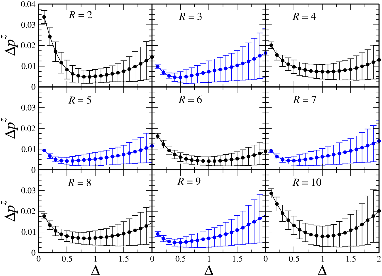
In Fig. 11 we show the integrated difference $\Delta p^{z}$. We see a slight dependence on whether $R$ is even or odd. Namely, for even values of $R$ the discrepancy between the ensembles at small values of $\Delta$ is more pronounced than for odd $R$. This effect is more visible for small values of $\Delta$. For even values of $R$ the difference $\Delta p^{z}$ has its smallest value for $\Delta=1$, while for odd values of $R$ the minimum is at $\Delta\sim 0.5$. Looking at the error bars, we see that both $p^{z}$ and $\Delta p^{z}$ are generally characterized by larger fluctuations with respect to the transverse spin, perhaps because the spectrum of $\sigma^{z}_{R}$ has a higher degeneracy with respect to $(S^{\perp}_{R})^{2}$. However the error bars, both for the transverse and longitudinal spin, are proportional to the disorder intensity. As we already pointed out for the transverse spin, we cannot fully characterize the dependence of $\Delta p^{z}$ on $R$, because we have too small systems. Intuitively, what we can expect is that the constraint on the total magnetization $\sum_{j}\sigma^{z}_{j}=0$ should relate the situations in which the subsystem has $R$ and $L-R$ sites respectively. On a qualitative level this is also suggested by the panels of Fig. 11.

References

- [1] Greiner M, Mandel O, Esslinger T, Hansch T and Bloch I 2002 Nature 415 39
- [2] Sadler L E, Higbie J M, Leslie S R, Vengalattore M and Stamper-Kurn D M 2006 Nature 443 312
- [3] Kinoshita T, Wenger T and Weiss D 2006 Nature 440 900
- [4] Deutsch J M 1991 Phys. Rev. A 43 2046
- [5] Srednicki M 1994 Phys. Rev. E 50 888
- [6] Zelevinsky V, Brown B A, Frazier N and Horoi M 1996 Phys. Rep. 276 85
- [7] Flambaum V V and Izrailev F M 1997 Phys. Rev. E 56 5144
- [8] Jacquod P and Shepelyansky D L 1997 Phys. Rev. Lett. 79 1837
- [9] Benenti G, Casati G and Shepelyansky D L 2001 Eur. Phys. J D 17 265
- [10] Polkovnikov A, Sengupta K, Silva A and Vengalattore M 2011 Rev. Mod. Phys. 83 863
- [11] Lamacraft A and Moore J 2011 arXiv: 1106.3567v1
- [12] Jaynes E T 1957 Phys. Rev. 106 620
- [13] Rigol M, Dunjko V, Yurovsky V and Olshanii M 2007 Phys. Rev. Lett. 98 050405
- [14] Rigol M, Dunjko V and Olshanii M 2008 Nature 452 854
- [15] Roux G 2009 Phys. Rev. A 79 021608
- [16] Biroli G, Kollath C and Läuchli A M 2010 Phys. Rev. Lett. 105 250401
- [17] Brandino G P, De Luca A, Konik R M and Mussardo G 2012 Phys. Rev. B 85 214435
- [18] Altshuler B L, Gefen Y, Kamenev A and Levitov L S 1997 Phys. Rev. Lett. 78 2803
- [19] Basko D M, Aleiner I L and Altshuler B L 2006 Ann. Phys. (NY) 321 1126
- [20] Gornyi I V, Mirlin A D and Polyakov D G 2005 Phys. Rev. Lett. 95 206603
- [21] Pal A and Huse D A 2010 Phys. Rev. B 82 174411
- [22] Canovi E, Rossini D, Fazio R, Santoro G E and Silva A 2011 Phys. Rev. B 83 094431
- [23] Carleo G, Becca F and Schirò M 2012 Sci. Rep. 2 243
- [24] Khatami E, Rigol M, Relaño A and García-García A M 2012 Phys. Rev. E 85 050102
- [25] Berges J, Borsányi S and Wetterich C 2004 Phys. Rev. Lett. 93 142002
- [26] Moeckel M and Kehrein S 2008 Phys. Rev. Lett. 100 175702
- [27] Moeckel M and Kehrein S 2010 New J. Phys. 12 055016
- [28] Eckstein M, Kollar M and Werner P 2009 Phys. Rev. Lett. 103 056403
- [29] Kollar M, Wolf F A and Eckstein M 2011 Phys. Rev. B 84 054304
- [30] Barnett R, Polkovnikov A and Vengalattore M 2011 Phys. Rev. A 84 023606
- [31] Mathey L and Polkovnikov A 2010 Phys. Rev. A 81 033605
- [32] Marino J and Silva A 2012 arXiv: 1203.2108
- [33] Gring M, Kuhnert M, Langen T, Kitagawa T, Rauer B, Schreitl M, Mazets I, Smith D A, Demler E and Schmiedmayer J 2011 arXiv: 1112.0013
- [34] Kitagawa T, Imambekov A, Schmiedmayer J and Demler E 2011 New J. Phys. 13 073018
- [35] Nagaosa N 1999 Quantum Field Theory in Strongly Correlated Electronic Systems (Berlin: Springer-Verlag)
- [36] Haldane F D M 1981 Phys. Rev. Lett. 47 1840
- [37] Bloch I, Dalibard J and Zwerger W 2008 Rev. Mod. Phys. 80 885
- [38] Doty C A and Fisher D S 1992 Phys. Rev. B 45 2167
- [39] Žnidaric M, Prosen T and Prelovšek P 2008 Phys. Rev. B 77 064426
- [40] Caux J S and Mossel J 2011 JSTAT P02023
- [41] Haake F 1991 Quantum Signatures of Chaos (Berlin: Springer-Verlag)
- [42] Di Stasio M and Zotos X 1995 Phys. Rev. Lett. 74 2050–2053
- [43] Kudo K and Deguchi T 2004 Phys. Rev. B 69 132404
- [44] Gómez J M G, Kar K, Kota V K B, Molina R A, Relaño A and Retamosa J 2011 Phys. Rep. 499 103
- [45] Brown W G, Santos L F, Starling D J and Viola L 2008 Phys. Rev. E 77 021106
- [46] Dukesz F, Zilbergerts M and Santos L F 2009 New J. Phys. 11 043026
- [47] Santos L F and Rigol M 2010 Phys. Rev. E 81 036206
- [48] Santos L F and Rigol M 2010 Phys. Rev. E 82 031130
- [49] Yurovsky V A and Olshanii M 2011 Phys. Rev. Lett. 106 025303
- [50] Santos L F, Borgonovi F and Izrailev F M 2012 Phys. Rev. Lett. 108 094102
- [51] Santos L F, Borgonovi F and Izrailev F M 2012 Phys. Rev. E 85 036209
- [52] Rossini D, Silva A, Mussardo G and Santoro G E 2009 Phys. Rev. Lett. 102 127204
- [53] Rossini D, Suzuki S, Mussardo G, Santoro G E and Silva A 2010 Phys. Rev. B 82 144302
- [54] Rigol M 2009 Phys. Rev. Lett. 103 100403
- [55] Rigol M and Santos L F 2010 Phys. Rev. A 82 011604
- [56] Polkovnikov A, Altman E and Demler E 2006 Proc. Natl. Acad. Sci. U.S.A. 103 6125
- [57] Gritsev V, Altman E, Demler E and Polkovnikov A 2006 Nat. Phys. 2 705
- [58] Kitagawa T, Pielawa S, Imambekov A, Schmiedmayer J, Gritsev V and Demler E 2010 Phys. Rev. Lett. 104 255302