跳到论文正文
W Papers独立论文阅读器 arXiv:1205.0368 论文正文 计算阅读时间 · 0%
引用这篇论文根据当前论文元数据生成,正式投稿前建议核对。


License: arXiv.org perpetual non-exclusive license
arXiv:1205.0368v1 [math.NA] 02 May 2012

A time-splitting spectral scheme for the Maxwell-Dirac systemThanks: This work was partially supported by the Wittgenstein Award 2000 of P. A. M., NSF grant No. DMS-0305080, the NSFC Projects no. 10301017 and 10228101, Basic Research Projects of Tsinghua University number JC 2002010, SRF for ROCS, SEM and the Austrian-Chinese Technical-Scientific Cooperation Agreement. C.S. has been supported by the APART grant of the Austrian Academy of Science.

Zhongyi Huang , Shi Jin , Peter A. Markowich , Christof Sparber and Chunxiong Zheng Z. Huang and C. ZhengDept. of Mathematical Sciences, Tsinghua University, Beijing 100084, China Email address: zhuang@math.tsinghua.edu.cn Email address: czheng@math.tsinghua.edu.cn S. JinDept. of Mathematics, University of Wisconsin, Madison, WI 53706, USA and Dept. of Mathematical Sciences, Tsinghua University, Beijing 100084, China Email address: jin@math.wisc.edu P. A. Markowich and C. SparberFakultät für Mathematik der Universität Wien
Nordbergstraße 15
A-1090 Vienna
Austria
Email address: peter.markowich@univie.ac.at Email address: christof.sparber@univie.ac.at
Abstract.

We present a time-splitting spectral scheme for the Maxwell-Dirac system and similar time-splitting methods for the corresponding asymptotic problems in the semi-classical and the non-relativistic regimes. The scheme for the Maxwell-Dirac system conserves the Lorentz gauge condition, is unconditionally stable and highly efficient as our numerical examples show. In particular we focus in our examples on the creation of positronic modes in the semi-classical regime and on the electron-positron interaction in the non-relativistic regime. Furthermore, in the non-relativistic regime, our numerical method exhibits uniform convergence in the small parameter δ\delta, which is the ratio of the characteristic speed and the speed of light.

Key words and phrases: 
Maxwell-Dirac system, time-splitting spectral method, semi-classical asymptotics, WKB-expansion, non-relativistic limit, Schrödinger-Poisson system
2000 Mathematics Subject Classification
81Q20, 35B25, 35B40, 35L60

version: August 24, 2026

1. Introduction and asymptotic scaling

The Maxwell-Dirac system (MD) describes the time-evolution of fast, i.e. relativistic spin-1/21/2 particles, say electrons and positrons, within external and self-consistent electromagnetic fields. In Lorentz gauge it is given by the following set of equations:

(1.1) {i¯h∂tψ=∑k=13αk(¯​h​ci∂k−q(Ak+Ake​x))ψ+q(V+Ve​x)ψ+mc2βψ,(1c2∂t​t−Δ)V=14​π​ϵ0ρ,(1c2∂t​t−Δ)𝐀=14​π​ϵ0​c𝐉,𝐱∈ℝ3,t∈ℝ,\left\{\begin{aligned} &i{\displaystyle\bar{\phantom{x}}\kern-6.0pth}\partial_{t}\psi=\sum_{k=1}^{3}\alpha^{k}\left(\frac{{\displaystyle\bar{\phantom{x}}\kern-6.0pth}c}{i}\partial_{k}-q(A_{k}+A_{k}^{ex})\right)\psi+q(V+V^{ex})\psi+mc^{2}\beta\psi,\\ &\left(\frac{1}{c^{2}}\partial_{tt}-\Delta\right)V=\frac{1}{4\pi\epsilon_{0}}\rho,\quad\left(\frac{1}{c^{2}}\partial_{tt}-\Delta\right)\boldsymbol{\rm{A}}=\frac{1}{4\pi\epsilon_{0}c}\,\boldsymbol{\rm{J}},\qquad\boldsymbol{\rm{x}}\in{\mathbb{R}}^{3},\ t\in{\mathbb{R}},\end{aligned}\right.

subject to Cauchy initial data:

(1.2) {V|t=0=V(0)(𝐱),∂tV|t=0=V(1)(𝐱),𝐀|t=0=𝐀(0)(𝐱),∂t𝐀|t=0=𝐀(1)(𝐱),ψ|t=0=ψ(0)(𝐱).\left\{\begin{aligned} &V\big|_{t=0}=V^{(0)}(\boldsymbol{\rm{x}}),\quad\,\partial_{t}V\big|_{t=0}=V^{(1)}(\boldsymbol{\rm{x}}),\\ &\boldsymbol{\rm{A}}\big|_{t=0}=\boldsymbol{\rm{A}}^{(0)}(\boldsymbol{\rm{x}}),\quad\partial_{t}\boldsymbol{\rm{A}}\big|_{t=0}=\boldsymbol{\rm{A}}^{(1)}(\boldsymbol{\rm{x}}),\quad\psi\big|_{t=0}=\psi^{(0)}(\boldsymbol{\rm{x}}).\end{aligned}\right.

The particle- and current-densities ρ\rho and 𝐉=(j1,j2,j3)\boldsymbol{\rm{J}}=(j_{1},j_{2},j_{3}) are defined by:

(1.3) ρ:=q|ψ|2,jk:=qc⟨ψ,αkψ⟩ℂ4≡qcψ¯⋅αkψ,k=1,2,3,\rho:=q|\psi|^{2},\quad j_{k}:=qc\langle\psi,\alpha^{k}\psi\rangle_{{\mathbb{C}}^{4}}\equiv qc\,\bar{\psi}\cdot\alpha^{k}\,\psi,\quad\ k=1,2,3,

where the spinor field ψ=ψ⁡(t,𝐱)=(ψ1,ψ2,ψ3,ψ4)T∈ℂ4\psi=\psi(t,\boldsymbol{\rm{x}})=(\psi_{1},\psi_{2},\psi_{3},\psi_{4})^{T}\in\mathbb{C}^{4} is normalized s.t.

(1.4) ∫ℝ3|ψ⁡(t,𝐱)|2​𝑑𝐱=1,\int_{\mathbb{R}^{3}}|\psi(t,\boldsymbol{\rm{x}})|^{2}d\boldsymbol{\rm{x}}=1,

with tt, 𝐱≡(x1,x2,x3)\boldsymbol{\rm{x}}\equiv(x_{1},x_{2},x_{3}), denoting the time - resp. spatial coordinates. Further, V⁡(t,𝐱)V(t,\boldsymbol{\rm{x}}) and Ve​x​(𝐱)∈ℝV^{ex}(\boldsymbol{\rm{x}})\in\mathbb{R} are the self-consistent resp. external electric potential and Ak​(t,𝐱)∈ℝA_{k}(t,\boldsymbol{\rm{x}})\in\mathbb{R}, resp. Ake​x​(𝐱)∈ℝA^{ex}_{k}(\boldsymbol{\rm{x}})\in\mathbb{R}, represents the kkth-components of the self-consistent, resp. external, magnetic potential, i.e. 𝐀=(A1,A2,A3)\rm\boldsymbol{\rm{A}}=(A_{1},A_{2},A_{3}). Here and in the following we shall only consider static external fields. The complex-valued, Hermitian Dirac matrices, i.e. β,αk\beta,\alpha^{k}, are explicitly given by:

(1.5) β:=(I​I200−I​I2),αk:=(0σkσk0),\beta:=\begin{pmatrix}{\rm I\kern-2.0ptI_{2}}&0\\ 0&-{\rm I\kern-2.0ptI_{2}}\end{pmatrix},\quad\alpha^{k}:=\begin{pmatrix}0&\sigma^{k}\\ \sigma^{k}&0\end{pmatrix},

with I​I2{\rm I\kern-2.0ptI_{2}}, the 2×22\times 2 identity matrix and σk\sigma^{k} the 2×22\times 2 Pauli matrices, i.e.

(1.6) σ1:=(0110),σ2:=(0−ii0),σ3:=(100−1).\sigma^{1}:=\begin{pmatrix}0&1\\ 1&0\end{pmatrix},\quad\sigma^{2}:=\begin{pmatrix}0&-i\\ i&0\end{pmatrix},\quad\sigma^{3}:=\begin{pmatrix}1&0\\ 0&-1\end{pmatrix}.

Finally, the physical constants, appearing in (1.1)-(1.3), are the normalized Planck’s constant ¯​h{\displaystyle\bar{\phantom{x}}\kern-6.0pth}, the speed of light cc, the permittivity of the vacuum ϵ0\epsilon_{0}, the particle mass mm and its charge qq.

Additionally to (1.1), we impose the Lorentz gauge condition

(1.7) ∂tV⁡(t,𝐱)+c​div⁡𝐀⁡(t,𝐱)=0,\partial_{t}V(t,\boldsymbol{\rm{x}})+c\diverg\boldsymbol{\rm{A}}(t,\boldsymbol{\rm{x}})=0,

for the initial potentials V(0)​(𝐱),V(1)​(𝐱)V^{(0)}(\boldsymbol{\rm{x}}),V^{(1)}(\boldsymbol{\rm{x}}), and 𝐀(0)​(𝐱),𝐀(1)​(𝐱)\boldsymbol{\rm{A}}^{(0)}(\boldsymbol{\rm{x}}),\boldsymbol{\rm{A}}^{(1)}(\boldsymbol{\rm{x}}). That means

1cV(1)(𝐱)+∇⋅𝐀(0)(𝐱)=0,ΔV(0)(𝐱)+q4​π​ϵ0|ψ(0)|2+1c∇⋅𝐀(1)(𝐱)=0.\frac{1}{c}V^{(1)}(\boldsymbol{\rm{x}})+\nabla\cdot\boldsymbol{\rm{A}}^{(0)}(\boldsymbol{\rm{x}})=0,\quad\Delta V^{(0)}(\boldsymbol{\rm{x}})+\frac{q}{4\pi\epsilon_{0}}|\psi^{(0)}|^{2}+\frac{1}{c}\nabla\cdot\boldsymbol{\rm{A}}^{(1)}(\boldsymbol{\rm{x}})=0.

Then the gauge is henceforth conserved during the time-evolution. This ensures that the corresponding electromagnetic fields 𝐄\boldsymbol{\rm{E}}, 𝐁\boldsymbol{\rm{B}} are uniquely determined by

(1.8) 𝐄(t,𝐱):=−1c∂t𝐀(t,𝐱)−∇V(t,𝐱),𝐁(t,𝐱):=curl𝐀(t,𝐱).\boldsymbol{\rm{E}}(t,\boldsymbol{\rm{x}}):=-\frac{1}{c}\partial_{t}\boldsymbol{\rm{A}}(t,\boldsymbol{\rm{x}})-\nabla V(t,\boldsymbol{\rm{x}}),\quad\boldsymbol{\rm{B}}(t,\boldsymbol{\rm{x}}):=\curl\boldsymbol{\rm{A}}(t,\boldsymbol{\rm{x}}).

Also it is easily seen that multiplying the Dirac equation with ψ¯\overline{\psi} implies the following conservation law

(1.9) ∂tρ+div⁡𝐉=0.\partial_{t}\rho+\diverg\boldsymbol{\rm{J}}=0.

The MD equations are the underlying field equations of relativistic quantum electro-dynamics, cf. [22], where one considers the system within the formalism of second quantization. Nevertheless, in order to obtain a deeper understanding for the interaction of matter and radiation, there is a growing interest in the MD system also for classical fields, since one can expect at least qualitative results, cf. [14]. Analytical results concerning local and global well-posedness of (1.1)-(1.3), have been obtained in [10, 11, 15, 16]. Also the rigorous study of asymptotic descriptions for the MD system has been a field of recent research. In particular the non-relativistic limit and the semi-classical asymptotic behavior (in the weakly coupled regime) have been discussed in [8, 23]. For the former case a numerical study can be found in [3]. Since our numerical simulations shall deal with both asymptotic regimes, let us discuss now more precisely the corresponding scaling for these physical situations.

1.1. The MD system in the (weakly coupled) semi-classical regime

First, we consider the semi-classical or high-frequency regime of fast (relativistic) particles, i.e. particles which have a reference speed v≈cv\approx c. (Of course for particles with mass m>0m>0 we always have v<cv<c.) To do so we rewrite the MD system in dimensionless form, such that there remains only one positive real parameter

(1.10) κ0=4​π​¯​h​c​ϵ0q2.\kappa_{0}=\frac{4\pi{\displaystyle\bar{\phantom{x}}\kern-6.0pth}c\epsilon_{0}}{q^{2}}.

As described in [23], we obtain the following rescaled MD system:

(1.11) {iκ0∂tψ=−iκ0𝜶⋅∇ψ−𝜶⋅(𝐀+𝐀e​x)ψ+(V+Ve​x)ψ+βψ,(∂t​t−Δ)V=ρ,(∂t​t−Δ)𝐀=𝐉,\left\{\begin{aligned} &i\kappa_{0}\,\partial_{t}\psi=-i\kappa_{0}\,\boldsymbol{\alpha}\cdot\nabla\psi-\boldsymbol{\alpha}\cdot(\boldsymbol{\rm{A}}+\boldsymbol{\rm{A}}^{ex})\psi+(V+V^{ex})\psi+\beta\psi,\\ &(\partial_{tt}-\Delta)V=\rho,\\ &(\partial_{tt}-\Delta)\boldsymbol{\rm{A}}=\boldsymbol{\rm{J}},\end{aligned}\right.

where from now on we shall also use the shorthand notation 𝜶⋅∇:=∑αk∂k\boldsymbol{\alpha}\cdot\nabla:=\sum\alpha^{k}\partial_{k}. Notice that if |q|=e|q|=e, i.e. in the case of electrons or positrons where qq equals the elementary charge ±e\pm e, the parameter κ0≈137\kappa_{0}\approx 137 is nothing but the reciprocal of the famous fine structure constant. Thus for fast (relativistic) particles which are not too heavily charged, κ0\kappa_{0} in general is not small and therefore asymptotic expansions as κ0→0\kappa_{0}\rightarrow 0 do not make sense. In order to describe the semi-classical regime we therefore suppose that the given external electromagnetic potentials are slowly varying w.r.t. the microscopic scales, i.e. Ve​x​t=Ve​x​t​(𝐱​ε/κ0)V^{ext}=V^{ext}(\boldsymbol{\rm{x}}{\varepsilon}/\kappa_{0}) and likewise Ae​x​t=Ae​x​t​(𝐱​ε/κ0)A^{ext}=A^{ext}(\boldsymbol{\rm{x}}{\varepsilon}/\kappa_{0}), where from now on 0<ε≪10<\varepsilon\ll 1 denotes the small semi-classical parameter. Here we fix κ0\kappa_{0} and include it in the scaling which conveniently eliminates this factor from the resulting equations. Finally, observing the time-evolution on macroscopic scales we are led to

(1.12) 𝐱~=εκ0​𝐱,t~=εκ0​t.\tilde{\boldsymbol{\rm{x}}}=\frac{\varepsilon}{\kappa_{0}}\boldsymbol{\rm{x}},\quad\tilde{t}=\frac{\varepsilon}{\kappa_{0}}t.

and we set

(1.13) ψε(t~,𝐱~)=(εκ0)−3/2ψ(t~κ0ε,𝐱~κ0ε)≡(εκ0)−3/2ψ(t,𝐱),\psi^{\varepsilon}(\tilde{t},\tilde{\boldsymbol{\rm{x}}})=\left(\frac{{\varepsilon}}{\kappa_{0}}\right)^{-3/2}\psi\left(\tilde{t}\frac{\kappa_{0}}{{\varepsilon}},\tilde{\boldsymbol{\rm{x}}}\frac{\kappa_{0}}{{\varepsilon}}\right)\equiv\left(\frac{{\varepsilon}}{\kappa_{0}}\right)^{-3/2}\psi(t,\boldsymbol{\rm{x}}),

in order to satisfy the normalization condition (1.4). Plugging this into (1.11) and omitting all “~\ \tilde{}\ ” we obtain the following semi-classically scaled MD system:

(1.14) {iε∂tψε=−iε𝜶⋅∇ψε−𝜶⋅(𝐀ε+𝐀e​x)ψε+(Vε+Ve​x)ψε+βψε,(∂t​t−Δ)Vε=ε|ψε|2,(∂t​t−Δ)Akε=ε⟨ψε,αkψε⟩ℂ4,k=1,2,3,\left\{\begin{aligned} &i{\varepsilon}\,\partial_{t}\psi^{\varepsilon}=-i{\varepsilon}\,\boldsymbol{\alpha}\cdot\nabla\psi^{\varepsilon}-\boldsymbol{\alpha}\cdot(\boldsymbol{\rm{A}}^{\varepsilon}+\boldsymbol{\rm{A}}^{ex})\psi^{\varepsilon}+(V^{\varepsilon}+V^{ex})\psi^{\varepsilon}+\beta\psi^{\varepsilon},\\ &(\partial_{tt}-\Delta)V^{\varepsilon}={\varepsilon}|\psi^{\varepsilon}|^{2},\\ &(\partial_{tt}-\Delta)A_{k}^{\varepsilon}={\varepsilon}\langle\psi^{\varepsilon},\alpha^{k}\psi^{\varepsilon}\rangle_{{\mathbb{C}}^{4}},\quad\ k=1,2,3,\end{aligned}\right.

with 0<ε≪10<{\varepsilon}\ll 1. Note the additional factor ε{\varepsilon} in the source terms appearing on the right hand side of the wave equations governing VεV^{\varepsilon} and 𝐀ε\boldsymbol{\rm{A}}^{\varepsilon}, which implies that we are dealing with a weak nonlinearity in the sense of [13, 21]. The scaled particle-density in this case is ρε:=|ψε|2\rho^{\varepsilon}:=|\psi^{\varepsilon}|^{2} and we also have 𝐉ε:=(⟨ψε,αk​ψε⟩ℂ4)k=1,2,3\boldsymbol{\rm{J}}^{\varepsilon}:=(\langle\psi^{\varepsilon},\alpha^{k}\psi^{\varepsilon}\rangle_{{\mathbb{C}}^{4}})_{k=1,2,3}.

Remark 1.1.

Note that, equivalently, we could consider small asymptotic solutions ψε∼𝒪⁡(ε)\psi^{\varepsilon}\sim\mathcal{O}(\sqrt{{\varepsilon}}) which again satisfy the semi-classical scaled MD system (1.14) but with source terms of order 𝒪⁡(1)\mathcal{O}(1) in the wave equations. This point of view is adopted in [23].

1.2. The MD system in the non-relativistic regime

We shall also deal with the non-relativistic regime for the MD system, i.e. we consider particles which have a reference speed v≪cv\ll c. Introducing a reference length LL, time TT and writing v=L/Tv=L/T, we rescale the time and the spatial coordinates in (1.1) by

(1.15) 𝐱~=𝐱L,t~=tT.\tilde{\boldsymbol{\rm{x}}}=\frac{\boldsymbol{\rm{x}}}{L},\quad\tilde{t}=\frac{t}{T}.

Moreover we set ψ~​(t~,𝐱~)=L3/2​ψ​(t,𝐱)\widetilde{\psi}(\tilde{t},\tilde{\boldsymbol{\rm{x}}})=L^{3/2}\psi(t,\boldsymbol{\rm{x}}), such that (1.4) is satisfied, and we also rescale the electromagnetic potentials by

(1.16) 𝐀~(e​x)​(t~,𝐱~)=λ​𝐀(e​x)​(t,𝐱),V~(e​x)​(t~,𝐱~)=λ​V(e​x)​(t,𝐱),\widetilde{\boldsymbol{\rm{A}}}^{(ex)}(\tilde{t},\widetilde{\boldsymbol{\rm{x}}})=\lambda\boldsymbol{\rm{A}}^{(ex)}(t,\boldsymbol{\rm{x}}),\quad\widetilde{V}^{(ex)}(\tilde{t},\widetilde{\boldsymbol{\rm{x}}})=\lambda V^{(ex)}(t,\boldsymbol{\rm{x}}),

where λ=q/(4​π​L​ε0)\lambda=q/(4\pi L{\varepsilon}_{0}), cf. [3, 6]. In this case we have again two important dimensionless parameters, namely

(1.17) δ=vc≪1,κ=4​π​¯​h​v​ε0q2.{\delta}=\frac{v}{c}\ll 1,\quad\kappa=\frac{4\pi{\displaystyle\bar{\phantom{x}}\kern-6.0pth}v\varepsilon_{0}}{q^{2}}.

Note that for v≈cv\approx c we get κ≈κ0\kappa\approx\kappa_{0}. Choosing for convenience v=q2/(4​π​¯​h​ε0)v=q^{2}/(4\pi{\displaystyle\bar{\phantom{x}}\kern-6.0pth}{\varepsilon}_{0}) and L=q/4​π​ε0L=q/4\pi{\varepsilon}_{0}, we shall from now on denote by ψδ​(t~,𝐱~)\psi^{\delta}(\tilde{t},\tilde{\boldsymbol{\rm{x}}}) the rescaled wave function ψ~​(t~,𝐱~)\widetilde{\psi}(\tilde{t},\tilde{\boldsymbol{\rm{x}}}), which is obtained for this particular choice of v=L/Tv=L/T. Then, similarly as before, ψδ\psi^{\delta} satisfies a dimensionless one-parameter model (again omitting all “~\ \tilde{}\ ”), given by

(1.18) {i∂tψδ=−iδ𝜶⋅∇ψδ−𝜶⋅(𝐀δ+𝐀e​x)ψδ+(Vδ+Ve​x)ψδ+1δ2βψδ,(δ2∂t​t−Δ)Vδ=|ψδ|2,(δ2∂t​t−Δ)Akδ=⟨ψδ,αkψδ⟩ℂ4,k=1,2,3.\left\{\begin{aligned} &i\partial_{t}\psi^{\delta}=-\frac{i}{{\delta}}\,\boldsymbol{\alpha}\cdot\nabla\psi^{\delta}-\boldsymbol{\alpha}\cdot(\boldsymbol{\rm{A}}^{\delta}+\boldsymbol{\rm{A}}^{ex})\psi^{\delta}+(V^{\delta}+V^{ex})\psi^{\delta}+\frac{1}{\delta^{2}}\beta\psi^{\delta},\\ &(\delta^{2}\partial_{tt}-\Delta)V^{\delta}=|\psi^{\delta}|^{2},\\ &({\delta}^{2}\partial_{tt}-\Delta)A_{k}^{\delta}=\langle\psi^{\delta},\alpha^{k}\psi^{\delta}\rangle_{{\mathbb{C}}^{4}},\quad\ k=1,2,3.\end{aligned}\right.

In analogy to the semi-classical case, this system will be called the non-relativistically scaled MD system. In this case the scaled particle density is ρδ:=|ψδ|2\rho^{\delta}:=|\psi^{\delta}|^{2}, whereas 𝐉δ:=δ−1​(⟨ψδ,αk​ψδ⟩ℂ4)k=1,2,3\boldsymbol{\rm{J}}^{\delta}:={\delta}^{-1}(\langle\psi^{\delta},\alpha^{k}\psi^{\delta}\rangle_{{\mathbb{C}}^{4}})_{k=1,2,3}. Note that in this scaling 𝐉δ∼𝒪⁡(1)\boldsymbol{\rm{J}}^{\delta}\sim\mathcal{O}(1), 𝐀δ∼𝒪⁡(δ)\boldsymbol{\rm{A}}^{\delta}\sim\mathcal{O}({\delta}), (due to a rather complex cancellation mechanism already known in the linear case cf. [6]) such that the magnetic field is a relativistic effect which does not appear in the zeroth order approximation of the MD system, cf. [6, 8, 19] (see also [7] for a similar study).

As in the corresponding numerical simulations for semi-classical nonlinear Schrödinger equations, cf. [1], the main difficulty is to find an efficient and convenient numerical scheme with best possible properties in the limiting regimes ε→0{\varepsilon}\to 0 and δ→0\delta\to 0, i.e. in particular with uniform convergence properties in δ{\delta}.

In the following we present a time-splitting spectral method for the MD system, and its semi-classical and non-relativistic limiting systems. The time-splitting spectral methods have been proved to be the best numerical approach to solve linear and nonlinear Schrödinger type systems in the semi-classical regime, cf. [1, 2]. Besides the usual properties of the time-splitting spectral method, such as the conservation of the Lorentz gauge condition and the unconditionally stability property, here we shall pay special attention to its performance in both the semi-classical and non-relativistic regimes. Note that in particular the semi-classical asymptotics has not been studied in [3]. The method proposed here is similar to the one used for the Zakharov system in [18]. A distinguished feature of the scheme developed in [18] is that it can be used, in the sub-sonic regime, with mesh size and time step independent of the subsonic parameter, a possibility not shared by works before [4, 5]. For the MD system, our time splitting spectral method allows the use of mesh size and time steps independent of the relativistic parameter δ\delta, allowing coarse grid computations in this asymptotic regime. This is achieved by the Crank-Nicolson time discretization for the Maxwell equations, a scheme shown to perform better for wave equations in the subsonic regime than the exact time integration, as studied in [18]. For the same reason, the previously proposed time-splitting spectral method for the MD system in [3] does not possess this property since it uses the exact time integration for the Maxwell equations.

The paper is now organized as follows: In section 2, we give the time-splitting spectral method for the MD system and one simple example to show the reliability, efficiency and the convergent rate of our method. Our method has spectral convergence for space discretization and second order convergence for time discretization. In section 3 and 4, we discuss the time-splitting methods for the asymptotic systems (the semi-classical regime and non-relativistic regime) and give some examples for them respectively. We conclude the paper in section 5.

2. A Time-splitting spectral method for the Maxwell-Dirac system

2.1. A time-splitting method

Before we describe our time-splitting spectral method, we combine the rescaled MD system (1.14) and (1.18), using two parameters:

(2.1) {iε∂tψ=−i​εδ𝜶⋅∇ψ−𝜶⋅(𝐀ε+𝐀e​x)ψ+(Vε+Ve​x)ψ+1δ2βψ,(δ2∂t​t−Δ)V=ε|ψ|2,(δ2∂t​t−Δ)Ak=ε⟨ψ,αkψ⟩ℂ4,k=1,2,3.\displaystyle\left\{\begin{aligned} &i{\varepsilon}\,\partial_{t}\psi=-\frac{i{\varepsilon}}{\delta}\,\boldsymbol{\alpha}\cdot\nabla\psi-\boldsymbol{\alpha}\cdot(\boldsymbol{\rm{A}}^{\varepsilon}+\boldsymbol{\rm{A}}^{ex})\psi+(V^{\varepsilon}+V^{ex})\psi+\frac{1}{\delta^{2}}\beta\psi,\\ &(\delta^{2}\partial_{tt}-\Delta)V={\varepsilon}|\psi|^{2},\\ &(\delta^{2}\partial_{tt}-\Delta)A_{k}={\varepsilon}\langle\psi,\alpha^{k}\psi\rangle_{{\mathbb{C}}^{4}},\quad\ k=1,2,3.\end{aligned}\right.

In the following we shall denote by

(2.2) 𝒟𝐀(D)ψ:=𝜶⋅(−i∇−𝐀e​x(𝐱))ψ+βψ+Ve​x(𝐱)ψ,\displaystyle\mathcal{D}_{\boldsymbol{\rm{A}}}(D)\psi:=\boldsymbol{\alpha}\cdot(-i\nabla-\boldsymbol{\rm{A}}^{ex}(\boldsymbol{\rm{x}}))\psi+\beta\psi+V^{ex}(\boldsymbol{\rm{x}})\psi,

the standard Dirac operator with (external) electromagnetic fields, D:=−i∇D:=-i\nabla. The corresponding 4×44\times 4 matrix-valued symbol is given by

(2.3) 𝒟𝐀​(ξ)=𝜶⋅(ξ−𝐀e​x​(𝐱))+β​ψ+Ve​x​(𝐱),\displaystyle\mathcal{D}_{\boldsymbol{\rm{A}}}(\xi)=\boldsymbol{\alpha}\cdot(\xi-\boldsymbol{\rm{A}}^{ex}(\boldsymbol{\rm{x}}))+\beta\psi+V^{ex}(\boldsymbol{\rm{x}}),\quad

where 𝐱,ξ∈ℝ3\boldsymbol{\rm{x}},\xi\in\mathbb{R}^{3}. Likewise the free Dirac operator will be written as

(2.4) 𝒟0(Dx)ψ:=−i𝜶⋅∇ψ+βψ\displaystyle\mathcal{D}_{0}(D_{x})\psi:=-i\boldsymbol{\alpha}\cdot\nabla\psi+\beta\psi

Its symbol admits a simple orthogonal decomposition given by

(2.5) 𝒟0​(ξ)≡α⋅ξ+β=λ0​(ξ)​Π0+​(ξ)−λ0​(ξ)​Π0−​(ξ),\displaystyle\mathcal{D}_{0}(\xi)\equiv\alpha\cdot\xi+\beta=\lambda_{0}(\xi)\Pi^{+}_{0}(\xi)-\lambda_{0}(\xi)\Pi_{0}^{-}(\xi),

where

(2.6) λ0​(ξ):=|ξ|2+1,\lambda_{0}(\xi):=\sqrt{|\xi|^{2}+1},

and

(2.7) Π0±​(ξ):=12​(I​I4±1λ0​(ξ)​𝒟0​(ξ)).\displaystyle\Pi_{0}^{\pm}(\xi):=\frac{1}{2}\left({\rm I\kern-2.0ptI_{4}}\pm\frac{1}{\lambda_{0}(\xi)}\mathcal{D}_{0}(\xi)\right).

The time-splitting scheme we propose is then as follows:

Step 1. Solve the system

(2.8) {i​ε​∂tψ−1δ2​𝒟0​(δ​ε​Dx)​ψ=0,(δ2∂t​t−Δ)V=ε|ψ|2,(δ2∂t​t−Δ)Ak=ε⟨ψ,αkψ⟩,k=1,2,3,\left\{\begin{aligned} &\,i{\varepsilon}\partial_{t}\psi-\frac{1}{{\delta}^{2}}\mathcal{D}_{0}({\delta}{\varepsilon}D_{x})\psi=0,\\ &\,({\delta}^{2}\partial_{tt}-\Delta)V={\varepsilon}|\psi|^{2},\\ &\,({\delta}^{2}\partial_{tt}-\Delta)A_{k}={\varepsilon}\left<\psi,\alpha^{k}\psi\right>,\quad k=1,2,3,\end{aligned}\right.

on a fixed time-interval △​t\triangle t, using the spectral decomposition (2.5).

Step 2. Then, in a second step we solve

(2.9) i​ε​∂tψ+𝜶⋅(𝐀+𝐀e​x)​ψ−(V+Ve​x)​ψ=0,\displaystyle i{\varepsilon}\partial_{t}\psi+\boldsymbol{\alpha}\cdot(\boldsymbol{\rm{A}}+\boldsymbol{\rm{A}}^{ex})\psi-(V+V^{ex})\psi=0,

on the same time-interval, where the solution obtained in step 1 serves as initial condition for step 2. Also the fields 𝐀\boldsymbol{\rm{A}}, VV are taken from step 1. It is then easy to see that this scheme conserves the particle density and the Lorentz gauge.

2.2. The numerical algorithm

In the following, for the convenience of computation, we shall deal with the system (2.1) on a bounded domain, for example, on the cubic domain

(2.10) Ω={𝐱=(x1,x2,x3)|aj≤xj≤bj,j=1,2,3},\displaystyle\Omega=\{\boldsymbol{\rm{x}}=(x_{1},x_{2},x_{3})\ |\ a_{j}\leq x_{j}\leq b_{j},j=1,2,3\},

imposing periodic boundary conditions. We choose the time step △​t=T/M\triangle t=T/M and spatial mesh size △​xj=(bj−aj)/Nj\triangle x_{j}=(b_{j}-a_{j})/N_{j}, j=1,2,3j=1,2,3, in xjx_{j}-direction, with given M,Nj∈ℕM,N_{j}\in{\mathbb{N}} and [0,T][0,T] denoting the computational time interval. Further we denote the time grid points by

(2.11) tn=n△t,tn+1/2=(n+12)△t,t=0,1,…,M\displaystyle t_{n}=n\triangle t,\quad t_{n+1/2}=\left(n+\frac{1}{2}\right)\triangle t,\quad t=0,1,\dots,M

and the spatial grid points by

(2.12) 𝐱𝐦=(x1,m1,x2,m2,x3,m3),where xj,mj:=aj+mj​△​xj,j=1,2,3,\displaystyle\mathbf{x}_{\mathbf{m}}=(x_{1,m_{1}},\ x_{2,m_{2}},\ x_{3,m_{3}}),\quad\mbox{where $x_{j,m_{j}}:=\,a_{j}+m_{j}\triangle x_{j}$},\quad j=1,2,3,

and 𝐦=(m1,m2,m3)∈ℳ\mathbf{m}=(m_{1},m_{2},m_{3})\in\mathcal{M}, with

(2.13) ℳ={(m1,m2,m3)| 0≤mj≤Nj,j=1,2,3}.\displaystyle\mathcal{M}=\,\left\{(m_{1},m_{2},m_{3})\,\Big|\ 0\leq m_{j}\leq N_{j},\ j=1,2,3\right\}.

In the following let Ψ𝐦n\Psi^{n}_{\mathbf{m}}, V𝐦nV^{n}_{\mathbf{m}}, and 𝐀𝐦n\mathbf{A}^{n}_{\mathbf{m}} be the numerical approximations of ψ⁡(tn,𝐱𝐦)\psi(t_{n},\mathbf{x}_{\mathbf{m}}), V⁡(tn,𝐱𝐦)V(t_{n},\mathbf{x}_{\mathbf{m}}), and 𝐀⁡(tn,𝐱𝐦)\mathbf{A}(t_{n},\mathbf{x}_{\mathbf{m}}), respectively. Suppose that we are given Ψn\Psi^{n}, VnV^{n}, and 𝐀n\mathbf{A}^{n}, then we obtain Ψn+1\Psi^{n+1}, Vn+1V^{n+1} and 𝐀n+1\mathbf{A}^{n+1} as follows:

Step 1. For the first step we denote the value of Ψ\Psi at time tt by Φ⁡(t)\Phi(t). Then we approximate the spatial derivative in (2.8) by the spectral differential operator. More precisely we first take a discrete Fourier transform (DFT) of (2.8):

(2.14) {∂tΦ^=−iε​δ2​(ε​δ​𝜶⋅ξ+β)​Φ^≡𝕄1​Φ^,(δ2∂t​t+|ξ|2)V^=ε|Φ|2^,(δ2∂t​t+|ξ|2)A^k=ε⟨Φ,αk​Φ⟩^,for k=1,2,3,\displaystyle\left\{\begin{aligned} &\,\partial_{t}\hat{\Phi}=-\frac{i}{{\varepsilon}\delta^{2}}\left({\varepsilon}\delta{\boldsymbol{\alpha}}\cdot\xi+\beta\right)\hat{\Phi}\equiv\mathbb{M}_{1}\hat{\Phi},\\ &\,({\delta}^{2}\partial_{tt}+|\xi|^{2})\hat{V}={\varepsilon}\widehat{\ |\Phi|^{2}},\\ &\,({\delta}^{2}\partial_{tt}+|\xi|^{2})\hat{A}_{k}={\varepsilon}\widehat{\left<\Phi,\alpha^{k}\Phi\right>},\quad\mbox{for }k=1,2,3,\end{aligned}\right.

where f^\hat{f} is the DFT of function ff. As the matrix 𝕄1∈ℂ4×4\mathbb{M}_{1}\in{\mathbb{C}}^{4\times 4} is diagonalizable, i.e. there exists a Hermitian matrix D1D_{1} such that

(2.15) D¯1T​𝕄1​D1=diag​[λ,λ,−λ,−λ]≡Λ\bar{D}_{1}^{T}\mathbb{M}_{1}D_{1}=\mbox{diag}\,[\lambda,\lambda,-\lambda,-\lambda]\equiv\Lambda

is a purely imaginary diagonal matrix with entries

(2.16) λ=iε​δ2​1+ε2​δ2​|ξ|2.\lambda=\frac{i}{{\varepsilon}\delta^{2}}\sqrt{1+{\varepsilon}^{2}\delta^{2}|\xi|^{2}}.

Then the value of Φ^\hat{\Phi} at time tn+1t_{n+1} is given by

(2.17) Φ^n+1\displaystyle\hat{\Phi}^{n+1} =\displaystyle= D1​exp⁡(Λ​△​t)​D¯1T​Ψ^n\displaystyle D_{1}\,\exp\left(\Lambda\triangle t\right)\,\bar{D}_{1}^{T}\hat{\Psi}^{n}
=\displaystyle= (cλ−i​sλ0−i​ε​δ​sλ​ξ3−ε​δ​sλ​(ξ2+i​ξ1)0cλ−i​sλε​δ​sλ​(ξ2−i​ξ1)i​ε​δ​sλ​ξ3−i​ε​δ​sλ​ξ3−ε​δ​s​(ξ2+i​ξ1)cλ+i​sλ0ε​δ​sλ​(ξ2−i​ξ1)i​ε​δ​sλ​ξ30cλ+i​sλ)​Ψ^n,\displaystyle\begin{pmatrix}c_{\lambda}-is_{\lambda}&0&-i{\varepsilon}\delta s_{\lambda}\xi_{3}&-{\varepsilon}\delta s_{\lambda}(\xi_{2}+i\xi_{1})\\ 0&c_{\lambda}-is_{\lambda}&{\varepsilon}\delta s_{\lambda}(\xi_{2}-i\xi_{1})&i{\varepsilon}\delta s_{\lambda}\xi_{3}\\ -i{\varepsilon}\delta s_{\lambda}\xi_{3}&-{\varepsilon}\delta s(\xi_{2}+i\xi_{1})&c_{\lambda}+is_{\lambda}&0\\ {\varepsilon}\delta s_{\lambda}(\xi_{2}-i\xi_{1})&i{\varepsilon}\delta s_{\lambda}\xi_{3}&0&c_{\lambda}+is_{\lambda}\\ \end{pmatrix}\hat{\Psi}^{n},

where

(2.18) cλ:=cos(−iλ△t),sλ:=sin(−iλ△t)(1+|εδξ|2)−1/2.c_{\lambda}:=\cos(-i\lambda\triangle t),\quad s_{\lambda}:=\sin(-i\lambda\triangle t)(1+|{\varepsilon}\delta\xi|^{2})^{-1/2}.

Then we obtain the value of Φn+1\Phi^{n+1} by an inverse discrete Fourier transform (IDFT). Hence from (2.14), we can find the values of V^\hat{V} and 𝐀^\hat{\mathbf{A}} by the Crank-Nicolson scheme, i.e.

(1+△​t2​|ξ|24​δ2)​(V^n+1∂tV^n+1)=(1−△​t2​|ξ|24​δ2△​t−△​t​|ξ|2δ21−△​t2​|ξ|24​δ2)​(V^n∂tV^n)+ε​(△​t24​δ2△​t2​δ2)​(ρ^n+ρ^n+1)\displaystyle\left(1+\frac{\triangle t^{2}|\xi|^{2}}{4\delta^{2}}\right)\left(\begin{array}[]{c}\hat{V}^{n+1}\\ \partial_{t}\hat{V}^{n+1}\end{array}\right)=\,\begin{pmatrix}1-\frac{\triangle t^{2}|\xi|^{2}}{4\delta^{2}}&\triangle t\\ -\frac{\triangle t|\xi|^{2}}{\delta^{2}}&1-\frac{\triangle t^{2}|\xi|^{2}}{4\delta^{2}}\end{pmatrix}\left(\begin{array}[]{c}\hat{V}^{n}\\ \partial_{t}\hat{V}^{n}\end{array}\right)+{\varepsilon}\left(\begin{array}[]{c}\frac{\triangle t^{2}}{4\delta^{2}}\\ \frac{\triangle t}{2\delta^{2}}\end{array}\right)\left(\hat{\rho}^{n}+\hat{\rho}^{n+1}\right)

and

(1+△​t2​|ξ|24​δ2)​(𝐀^n+1∂t𝐀^n+1)=(1−△​t2​|ξ|24​δ2△​t−△​t​|ξ|2δ21−△​t2​|ξ|24​δ2)​(𝐀^n∂t𝐀^n)+ε​δ​(△​t24​δ2△​t2​δ2)​(𝐉^n+𝐉^n+1),\displaystyle\left(1+\frac{\triangle t^{2}|\xi|^{2}}{4\delta^{2}}\right)\left(\begin{array}[]{c}\hat{\mathbf{A}}^{n+1}\\ \partial_{t}\hat{\boldsymbol{\rm{A}}}^{n+1}\end{array}\!\!\!\right)=\,\begin{pmatrix}1-\frac{\triangle t^{2}|\xi|^{2}}{4\delta^{2}}&\triangle t\\ -\frac{\triangle t|\xi|^{2}}{\delta^{2}}&1-\frac{\triangle t^{2}|\xi|^{2}}{4\delta^{2}}\end{pmatrix}\left(\!\!\begin{array}[]{c}\hat{\boldsymbol{\rm{A}}}^{n}\\ \partial_{t}\hat{\boldsymbol{\rm{A}}}^{n}\end{array}\right)+{\varepsilon}{\delta}\left(\!\!\begin{array}[]{c}\frac{\triangle t^{2}}{4\delta^{2}}\\ \frac{\triangle t}{2\delta^{2}}\end{array}\right)\left(\hat{\boldsymbol{\rm{J}}}^{n}+\hat{\boldsymbol{\rm{J}}}^{n+1}\right),

where for k=1,2,3k=1,2,3, we denote

(2.31) ρn=|Ψn|2,ρn+1=|Φn+1|2,𝐉kn=δ−1​⟨Ψn,αk​Ψn⟩,𝐉kn+1=δ−1​⟨Φn+1,αk​Φn+1⟩.\displaystyle\rho^{n}=|\Psi^{n}|^{2},\ \rho^{n+1}=|\Phi^{n+1}|^{2},\ \boldsymbol{\rm{J}}_{k}^{n}={\delta}^{-1}\left<\Psi^{n},\alpha^{k}\Psi^{n}\right>,\ \boldsymbol{\rm{J}}_{k}^{n+1}={\delta}^{-1}\left<\Phi^{n+1},\alpha^{k}\Phi^{n+1}\right>.

Performing an IDFT of V^n+1\hat{V}^{n+1} and 𝐀^n+1\hat{\mathbf{A}}^{n+1}, we finally obtain Vn+1V^{n+1} and 𝐀n+1\mathbf{A}^{n+1}.

Step 2. Since VV and AkA_{k} do not change in Step 2, we only have to update Ψ\Psi. First we shall rewrite the equation (2.9) in the following form:

(2.32) ∂tΨ=iε​𝜶⋅(𝐀+𝐀e​x)​Ψ−(V+Ve​x)​Ψ≡𝕄2​Ψ.\partial_{t}\Psi=\frac{i}{{\varepsilon}}\,\boldsymbol{\alpha}\cdot(\boldsymbol{\rm{A}}+\boldsymbol{\rm{A}}^{ex})\Psi-(V+V^{ex})\Psi\equiv\mathbb{M}_{2}\Psi.

Then there exists again a Hermitian matrix D2D_{2} such that

(2.33) D¯2T​𝕄2​D2=diag​[μ1,μ1,μ2,μ2]≡Θ,\bar{D}_{2}^{T}\mathbb{M}_{2}D_{2}=\mbox{diag}\,[\mu_{1},\mu_{1},\mu_{2},\mu_{2}]\equiv\Theta,

where Θ\Theta is a purely imaginary diagonal matrix with

(2.34) μ1=−iε​((V+Ve​x)−|𝐀+𝐀e​x|),μ2=−iε​((V+Ve​x)+|𝐀+𝐀e​x|).\mu_{1}=-\frac{i}{{\varepsilon}}\left((V+V^{ex})-|\mathbf{A}+\mathbf{A}^{ex}|\right),\quad\mu_{2}=-\frac{i}{{\varepsilon}}\left((V+V^{ex})+|\mathbf{A}+\mathbf{A}^{ex}|\right).

Hence, the value of Ψ\Psi at time tn+1t_{n+1} is given by

(2.35) Ψn+1\displaystyle\Psi^{n+1} =\displaystyle= D2​exp⁡(Θ​△​t)​D¯2T​Φn+1\displaystyle D_{2}\,\exp\left(\Theta\triangle t\right)\,\bar{D}_{2}^{T}\Phi^{n+1}
=\displaystyle= (c1+c2−i⁡(s1+s2)20A3|𝐀|​(c0−i​s0)A1−i​A2|𝐀|​(c0−i​s0)0c1+c2−i⁡(s1+s2)2A1+i​A2|𝐀|​(c0−i​s0)−A3|𝐀|​(c0−i​s0)A3|𝐀|​(c0−i​s0)A1−i​A2|𝐀|​(c0−i​s0)c1+c2−i⁡(s1+s2)20A1+i​A2|𝐀|​(c0−i​s0)−A3|𝐀|​(c0−i​s0)0c1+c2−i⁡(s1+s2)2)​Φn+1,\displaystyle\begin{pmatrix}\frac{c_{1}+c_{2}-i(s_{1}+s_{2})}{2}&0&\frac{A_{3}}{|\boldsymbol{\rm{A}}|}(c_{0}-is_{0})&\frac{A_{1}-iA_{2}}{|\boldsymbol{\rm{A}}|}(c_{0}-is_{0})\\ 0&\frac{c_{1}+c_{2}-i(s_{1}+s_{2})}{2}&\frac{A_{1}+iA_{2}}{|\boldsymbol{\rm{A}}|}(c_{0}-is_{0})&-\frac{A_{3}}{|\boldsymbol{\rm{A}}|}(c_{0}-is_{0})\\ \frac{A_{3}}{|\boldsymbol{\rm{A}}|}(c_{0}-is_{0})&\frac{A_{1}-iA_{2}}{|\boldsymbol{\rm{A}}|}(c_{0}-is_{0})&\frac{c_{1}+c_{2}-i(s_{1}+s_{2})}{2}&0\\ \frac{A_{1}+iA_{2}}{|\boldsymbol{\rm{A}}|}(c_{0}-is_{0})&-\frac{A_{3}}{|\boldsymbol{\rm{A}}|}(c_{0}-is_{0})&0&\frac{c_{1}+c_{2}-i(s_{1}+s_{2})}{2}\\ \end{pmatrix}\Phi^{n+1},

where we use a notation analogous to (2.18) and write

(2.36) exp⁡(μ1​△​t)≡c1−i​s1,exp⁡(μ2​△​t)≡c2−i​s2,c0:=c1−c2,s0:=s1−s2.\exp(\mu_{1}\triangle t)\equiv c_{1}-is_{1},\ \exp(\mu_{2}\triangle t)\equiv c_{2}-is_{2},\ c_{0}:=c_{1}-c_{2},\ s_{0}:=s_{1}-s_{2}.

Clearly, the algorithm given above is first order in time. We can get a second order scheme by the Strang splitting method, which means that we use Step 1 with time-step △​t/2\triangle t/2, then Step 2 with time-step △​t\triangle t, and finally integrate Step 1 again with △​t/2\triangle t/2. Our algorithm given above is an ‘explicit’ and unconditional stable scheme. The main costs are DFT and IDFT.

Lemma 2.1.

Our numerical scheme conserves the particle density in the discrete l2l^{2} norm (discrete total charge) and the Lorentz gauge.

Proof: From (2.17) and (2.35), it is easy to check that the discrete total charge is conserved. From the initial conditions and (2.2), we have

δ​∂tV^0+i​ξ⋅𝐀^0=0,ε​ρ^0=|ξ|2​V^0−i​δ​ξ⋅∂t𝐀^0,ρ^1=ρ^0−i​△​t2​δ​ξ⋅(𝐉^0+𝐉^1).\delta\partial_{t}\hat{V}^{0}+i\xi\cdot\hat{\boldsymbol{\rm{A}}}^{0}=0,\quad\varepsilon\hat{\rho}^{0}=|\xi|^{2}\hat{V}^{0}-i\delta\xi\cdot\partial_{t}\hat{\boldsymbol{\rm{A}}}^{0},\quad\hat{\rho}^{1}=\hat{\rho}^{0}-\frac{i\triangle t}{2\delta}\xi\cdot\left(\hat{\boldsymbol{\rm{J}}}^{0}+\hat{\boldsymbol{\rm{J}}}^{1}\right).

From (2.2) and (2.2), we obtain

(1+△​t2​|ξ|24​δ2)​(δ​∂tV^n+1+i​ξ⋅𝐀^n+1)\displaystyle\left(1+\frac{\triangle t^{2}|\xi|^{2}}{4\delta^{2}}\right)\left(\delta\partial_{t}\hat{V}^{n+1}+i\xi\cdot\hat{\boldsymbol{\rm{A}}}^{n+1}\right) =\displaystyle= (1−△​t2​|ξ|24​δ2)​(δ​∂tV^n+i​ξ⋅𝐀^n)\displaystyle\left(1-\frac{\triangle t^{2}|\xi|^{2}}{4\delta^{2}}\right)\left(\delta\partial_{t}\hat{V}^{n}+i\xi\cdot\hat{\boldsymbol{\rm{A}}}^{n}\right)
+\displaystyle+ △​tδ​(−|ξ|2​V^n+i​δ​ξ⋅∂t𝐀^n)\displaystyle\frac{\triangle t}{\delta}\left(-|\xi|^{2}\hat{V}^{n}+i\delta\xi\cdot\partial_{t}\hat{\boldsymbol{\rm{A}}}^{n}\right)
+\displaystyle+ ε​△​t2​δ​(ρ^n+ρ^n+1+i​△​t2​δ​ξ⋅(𝐉^n+𝐉^n+1)).\displaystyle\frac{\varepsilon\triangle t}{2\delta}\left(\hat{\rho}^{n}+\hat{\rho}^{n+1}+\frac{i\triangle t}{2\delta}\xi\cdot\left(\hat{\boldsymbol{\rm{J}}}^{n}+\hat{\boldsymbol{\rm{J}}}^{n+1}\right)\right).

Then it is clear that for all nn, we have

δ∂tV^n+iξ⋅𝐀^n=0,ερ^n=|ξ|2V^n−iδξ⋅∂t𝐀^n,ρ^n+1=ρ^n−i​△​t2​δξ⋅(𝐉^n+𝐉^n+1).□\delta\partial_{t}\hat{V}^{n}+i\xi\cdot\hat{\boldsymbol{\rm{A}}}^{n}=0,\quad\varepsilon\hat{\rho}^{n}=|\xi|^{2}\hat{V}^{n}-i\delta\xi\cdot\partial_{t}\hat{\boldsymbol{\rm{A}}}^{n},\quad\hat{\rho}^{n+1}=\hat{\rho}^{n}-\frac{i\triangle t}{2\delta}\xi\cdot\left(\hat{\boldsymbol{\rm{J}}}^{n}+\hat{\boldsymbol{\rm{J}}}^{n+1}\right).\quad\Box

In order to test the numerical scheme we consider the example of an exact solution for the full MD system, cf. [12]. In all of the following examples, we take the computational domain Ω\Omega to be the unit cubic [−0.5,0.5]3[-0.5,0.5]^{3}.

Example 2.1 (Exact solution for the MD system).

Let us consider the MD system for ε=δ=1{\varepsilon}=\delta=1 with initial data

(2.37) {ψ(0)(𝐱)=exp⁡(i​ξ⋅𝐱)2​(1+|ξ|2−1+|ξ|2)χ,χ=(ξ3,ξ1+iξ2,1+|ξ|2−1,0),V(0)(𝐱)=V(1)(𝐱)=0,𝐀(0)(𝐱)=𝐀(1)(𝐱)=0,\left\{\begin{aligned} &\psi^{(0)}(\boldsymbol{\rm{x}})=\displaystyle\frac{\exp(i\xi\cdot\boldsymbol{\rm{x}})}{\sqrt{2(1+|\xi|^{2}-\sqrt{1+|\xi|^{2}})}}\ \chi,\quad\chi=(\xi_{3},\xi_{1}+i\xi_{2},\sqrt{1+|\xi|^{2}}-1,0),\\ &V^{(0)}(\boldsymbol{\rm{x}})=V^{(1)}(\boldsymbol{\rm{x}})=0,\quad\boldsymbol{\rm{A}}^{(0)}(\boldsymbol{\rm{x}})=\boldsymbol{\rm{A}}^{(1)}(\boldsymbol{\rm{x}})=0,\end{aligned}\right.

and external fields given by

(2.38) Ve​x=−t22,𝐀e​x=−t2​ξ2​1+|ξ|2,ξ=(2​π,4​π,6​π)∈ℝ3.V^{ex}=\displaystyle-\frac{t^{2}}{2},\qquad\boldsymbol{\rm{A}}^{ex}=-\frac{t^{2}\xi}{2\sqrt{1+|\xi|^{2}}},\quad\xi=(2\pi,4\pi,6\pi)\in{\mathbb{R}}^{3}.

In this case, there is an exact plane wave solutions for the MD system in the following form, cf. [12]:

(2.39) {ψ⁡(t,𝐱)=exp⁡(i⁡(ξ⋅𝐱−t​1+|ξ|2))2​(1+|ξ|2−1+|ξ|2)​χ,V⁡(t,𝐱)=t22,𝐀(t,𝐱)=t2​ξ2​1+|ξ|2.\left\{\begin{aligned} \psi(t,\boldsymbol{\rm{x}})&=\displaystyle\frac{\exp\big(i(\xi\cdot\boldsymbol{\rm{x}}-t\sqrt{1+|\xi|^{2}})\big)}{\sqrt{2(1+|\xi|^{2}-\sqrt{1+|\xi|^{2}})}}\ \chi,\\ V(t,\boldsymbol{\rm{x}})&=\displaystyle\frac{t^{2}}{2},\quad\boldsymbol{\rm{A}}(t,\boldsymbol{\rm{x}})=\frac{t^{2}\xi}{2\sqrt{1+|\xi|^{2}}}.\end{aligned}\right.

In Figure 1, we see that our method gives a very good agreement with the exact result.

Figure 1. The numerical solutions of example 2.1. Here △​t=1128\triangle t=\frac{1}{128}, △​x=132\triangle x=\frac{1}{32}. The top two graphs are the real and imaginary parts of ψ1ε​(t,0,x2,0)|t=1\psi^{\varepsilon}_{1}(t,0,x_{2},0)|_{t=1}. The bottom two graphs are electromagnetic potentials and the norms of ψkε\psi^{\varepsilon}_{k}, k=1,2,3,4k=1,2,3,4. The solid lines are the exact solutions, ‘ooo’, ‘***’, ‘⋄⋄⋄\diamond\diamond\diamond’ and ‘□​□​□\square\square\square’ are numerical solutions.

To test the accuracy of our time-splitting method for the MD system, we did the spatial and temporal discretization error tests (see Table 1 and 2). Table 1 shows the spectral convergence for spatial discretization. Table 2 shows the convergence rate for temporal discretization is about 2.0. Here ψ△​x,△​t​(t,⋅)\psi^{\triangle x,\triangle t}(t,\cdot) is the numerical solution for mesh size △​x\triangle x and time step △​t\triangle t, and ψ⁡(t,⋅)\psi(t,\cdot) is the exact solution given by (2.39). In the following also show the charge conservation test (see Table 3):

Table 1. Spatial discretization error test: at time t=0.25 under △​t=1/1024\triangle t=1/1024 (ε=δ=1{\varepsilon}=\delta=1).
mesh size △​x=1/4\triangle x=1/4 △​x=1/8\triangle x=1/8 △​x=1/16\triangle x=1/16 △​x=1/32\triangle x=1/32
‖ψ△​x,△​t​(t,⋅)−ψ⁡(t,⋅)‖l2‖ψ⁡(t,⋅)‖l2\begin{array}[]{c}\\ \displaystyle\frac{{\left\|\psi^{\triangle x,\triangle t}(t,\cdot)-\psi(t,\cdot)\right\|}_{l^{2}}}{{\|\psi(t,\cdot)\|}_{l^{2}}}\\ \end{array} 8.40E-2 2.68E-3 6.95E-5 5.00E-8
convergence order 4.9 5.3 10.4
Table 2. Temporal discretization error test: at time t=0.25 under △​x=1/32\triangle x=1/32 (ε=δ=1{\varepsilon}=\delta=1).
time step △​t=116\triangle t=\frac{1}{16} △​t=132\triangle t=\frac{1}{32} △​t=164\triangle t=\frac{1}{64} △​t=1128\triangle t=\frac{1}{128}
‖ψ△​x,△​t​(t,⋅)−ψ⁡(t,⋅)‖l2‖ψ⁡(t,⋅)‖l2\begin{array}[]{c}\\ \displaystyle\frac{{\left\|\psi^{\triangle x,\triangle t}(t,\cdot)-\psi(t,\cdot)\right\|}_{l^{2}}}{{\|\psi(t,\cdot)\|}_{l^{2}}}\\ \end{array} 2.59E-4 5.14E-5 1.29E-5 3.21E-6
convergence order 2.3 2.0 2.0
Table 3. Charge conservation test: under △​x=1/32\triangle x=1/32, △​t=1/1024\triangle t=1/1024 (ε=δ=1{\varepsilon}=\delta=1).
time t=0 t=0.5 t=1.0
‖ψ△​x,△​t​(t,⋅)‖l2{\|\psi^{\triangle x,\triangle t}(t,\cdot)\|_{l^{2}}} 1.00000000 0.99999998 0.99999997

3. The semi-classical regime

We shall consider in the following the semi-classically scaled MD system (1.14). First we shall discuss the (formal) asymptotic description as ε→0{\varepsilon}\rightarrow 0 and then consider some particular numerical test cases.

3.1. Formal asymptotic description

To describe the limiting behavior of ψε\psi^{\varepsilon} as ε→0{\varepsilon}\rightarrow 0 we introduce the following notations:

Analogously to the free Dirac operator, the matrix-valued symbol 𝒟𝐀​(ξ)\mathcal{D}_{\boldsymbol{\rm{A}}}(\xi) can be (orthogonally) decomposed into

(3.1) 𝒟𝐀​(ξ)=h𝐀+​(ξ)​Π𝐀+​(ξ)+h𝐀−​(ξ)​Π𝐀−​(ξ),ξ∈ℝ3,\displaystyle\mathcal{D}_{\boldsymbol{\rm{A}}}(\xi)=h_{\boldsymbol{\rm{A}}}^{+}(\xi)\Pi^{+}_{\boldsymbol{\rm{A}}}(\xi)+h_{\boldsymbol{\rm{A}}}^{-}(\xi)\Pi_{\boldsymbol{\rm{A}}}^{-}(\xi),\quad\xi\in\mathbb{R}^{3},

where

(3.2) h𝐀±​(ξ):=±λ𝐀​(ξ)+V⁡(𝐱),\displaystyle h^{\pm}_{\boldsymbol{\rm{A}}}(\xi):=\pm\lambda_{\boldsymbol{\rm{A}}}(\xi)+V(\boldsymbol{\rm{x}}),

with

(3.3) λ𝐀​(ξ):=1+|ξ−𝐀e​x​(𝐱)|2+Ve​x​(𝐱).\displaystyle\lambda_{\boldsymbol{\rm{A}}}(\xi):=\sqrt{{1+|\xi-\boldsymbol{\rm{A}}^{ex}(\boldsymbol{\rm{x}})|}^{2}}+V^{ex}(\boldsymbol{\rm{x}}).

The corresponding (orthogonal) projectors Π𝐀±​(ξ)\Pi_{\boldsymbol{\rm{A}}}^{\pm}(\xi) are then given by

(3.4) Π𝐀±​(ξ):=12​(I​I4±1λ𝐀​(ξ)​(𝒟𝐀​(ξ)−Ve​x​(𝐱)​I​I4)).\displaystyle\Pi_{\boldsymbol{\rm{A}}}^{\pm}(\xi):=\frac{1}{2}\left({\rm I\kern-2.0ptI_{4}}\pm\frac{1}{\lambda_{\boldsymbol{\rm{A}}}(\xi)}\ \left(\mathcal{D}_{\boldsymbol{\rm{A}}}(\xi)-V^{ex}(\boldsymbol{\rm{x}}){\rm I\kern-2.0ptI_{4}}\right)\right).

Clearly, we obtain the corresponding decomposition of the free Dirac operator (2.5), (2.7), by setting 𝐀e​x​(𝐱)=0\boldsymbol{\rm{A}}^{ex}(\boldsymbol{\rm{x}})=0 and Ve​x​(𝐱)=0V^{ex}(\boldsymbol{\rm{x}})=0 in the above formulas. Note that h𝐀±​(ξ)h^{\pm}_{\boldsymbol{\rm{A}}}(\xi) is nothing but the classical relativistic Hamiltonian (corresponding to positive resp. negative energies) for a particle with momentum ξ\xi. These particles can be interpreted as positrons and electrons, resp., at least in the limit ε→0{\varepsilon}\rightarrow 0, as we shall see below. Finally, we also define the relativistic group-velocity by

(3.5) ω𝐀±​(ξ):=∇ξh𝐀±​(ξ).\omega_{\boldsymbol{\rm{A}}}^{\pm}(\xi):=\nabla_{\xi}h^{\pm}_{\boldsymbol{\rm{A}}}(\xi).

The group velocity for free relativistic particles is then ω0±​(ξ)=ξ/λ0​(ξ)\omega_{0}^{\pm}(\xi)=\xi/\lambda_{0}(\xi).

The semi-classical limit for solution of the weakly nonlinear MD system (1.14) can now be described by means of WKB-techniques as given in [23] (see also [24]) . To do so we assume (well prepared) highly oscillatory initial data for ψε\psi^{\varepsilon}, i.e.

(3.6) ψ(0)​(𝐱)∼uI+​(𝐱)​ei​ϕI+​(𝐱)/ε+uI−​(𝐱)​ei​ϕI−​(𝐱)/ε+𝒪⁡(ε).\psi^{(0)}(\boldsymbol{\rm{x}})\sim u^{+}_{I}(\boldsymbol{\rm{x}})e^{i\phi^{+}_{I}(\boldsymbol{\rm{x}})/{\varepsilon}}+u^{-}_{I}(\boldsymbol{\rm{x}})e^{i\phi^{-}_{I}(\boldsymbol{\rm{x}})/{\varepsilon}}+\mathcal{O}({\varepsilon}).

We then expect that ψε​(t,𝐱)\psi^{\varepsilon}(t,\boldsymbol{\rm{x}}) can be described in leading order (as ε→0{\varepsilon}\rightarrow 0) by a WKB-approximation of the following form

(3.7) ψε​(t,𝐱)∼u+​(t,𝐱)​ei​ϕ+​(t,𝐱)/ε+u−​(t,𝐱)​ei​ϕ−​(t,𝐱)/ε+𝒪⁡(ε).\displaystyle\psi^{\varepsilon}(t,\boldsymbol{\rm{x}})\sim u^{+}(t,\boldsymbol{\rm{x}})e^{i\phi^{+}(t,\boldsymbol{\rm{x}})/\varepsilon}+u^{-}(t,\boldsymbol{\rm{x}})e^{i\phi^{-}(t,\boldsymbol{\rm{x}})/\varepsilon}+\mathcal{O}({\varepsilon}).

Here, the phase functions ϕ±​(t,𝐱)∈ℝ\phi^{\pm}(t,\boldsymbol{\rm{x}})\in{\mathbb{R}}, resp. satisfy the electronic or positronic eiconal equation

(3.8) ∂tϕ±​(t,𝐱)+h𝐀±​(∇ϕ±​(t,𝐱))=0,ϕ±​(0,𝐱)=ϕI±​(𝐱).\partial_{t}\phi^{\pm}(t,\boldsymbol{\rm{x}})+h^{\pm}_{\boldsymbol{\rm{A}}}(\nabla\phi^{\pm}(t,\boldsymbol{\rm{x}}))=0,\quad\phi^{\pm}(0,\boldsymbol{\rm{x}})=\phi^{\pm}_{I}(\boldsymbol{\rm{x}}).

As usual in WKB-analysis we can expect an approximation of the form (3.7) to be valid only locally in time, i.e. for |t|<tc|t|<t_{c}, where tct_{c} denotes the time at which the first caustic appears in the solution of (3.8).

Remark 3.1.

We want to stress that the self-consistent fields 𝐀ε\boldsymbol{\rm{A}}^{\varepsilon}, VεV^{\varepsilon} do not enter in (3.8), i.e. the eiconal equation is found to be the same as in the linear case. This is due to the weakly nonlinear scaling described in the introduction. In particular, i.e. for the Dirac equation without Maxwell coupling, this setting allows us to compute the rays of geometrical optics, i.e. the characteristics for (3.8), independently of 𝐀ε\boldsymbol{\rm{A}}^{\varepsilon}, VεV^{\varepsilon}.

It is shown in [23], for the simplified case where 𝐀e​x​(𝐱)=Ve​x​(𝐱)=0\boldsymbol{\rm{A}}^{ex}(\boldsymbol{\rm{x}})=V^{ex}(\boldsymbol{\rm{x}})=0, that the principal-amplitudes u±​(t,𝐱)∈ℂ4u^{\pm}(t,\boldsymbol{\rm{x}})\in{\mathbb{C}}^{4} solve a nonlinear first order system, given by

(3.9) {(∂t+(ω0+(∇ϕ+)⋅∇))u++12div(ω0+(∇ϕ+))u+=i𝒩+[u]u+,(∂t+(ω0−(∇ϕ−)⋅∇))u−+12div(ω0−(∇ϕ−))u−=i𝒩−[u]u−,\left\{\begin{aligned} &\,\left(\partial_{t}+(\omega_{0}^{+}(\nabla\phi^{+})\cdot\nabla)\right)u^{+}+\frac{1}{2}\diverg(\omega_{0}^{+}(\nabla\phi^{+}))u^{+}=i\mathcal{N}^{+}[u]\,u^{+},\\ &\,\left(\partial_{t}+(\omega_{0}^{-}(\nabla\phi^{-})\cdot\nabla)\right)u^{-}+\frac{1}{2}\diverg(\omega_{0}^{-}(\nabla\phi^{-}))u^{-}=i\mathcal{N}^{-}[u]\,u^{-},\\ \end{aligned}\right.

with initial condition

(3.10) u±​(0,𝐱):=Π0±​(∇ϕI±)​uI​(𝐱).u^{\pm}(0,\boldsymbol{\rm{x}}):=\Pi_{0}^{\pm}(\nabla\phi_{I}^{\pm})u_{I}(\boldsymbol{\rm{x}}).

The nonlinearity on the r.h.s. of (3.9) is given by

(3.11) 𝒩±​[u]:=𝒜⋅ω0±​(∇ϕ±)−𝒱,\mathcal{N}^{\pm}[u]:=\mathcal{A}\cdot\omega_{0}^{\pm}(\nabla\phi^{\pm})-\mathcal{V},

where the fields 𝒱\mathcal{V}, 𝒜\mathcal{A} are computed self-consistently through

(3.12) (∂t​t−Δ)𝒱=ρ0,(∂t​t−Δ)𝒜=𝐉0.\displaystyle(\partial_{tt}-\Delta)\mathcal{V}=\rho^{0},\quad(\partial_{tt}-\Delta)\mathcal{A}=\boldsymbol{\rm{J}}^{0}.

with source terms

(3.13) ρ0:=|u+|2+|u−|2,𝐉0:=ω0+​(∇ϕ+)​|u+|2+ω0−​(∇ϕ−)​|u−|2.\displaystyle\rho^{0}:=|u^{+}|^{2}+|u^{-}|^{2},\quad\boldsymbol{\rm{J}}^{0}:=\omega_{0}^{+}(\nabla\phi^{+})|u^{+}|^{2}\ +\omega_{0}^{-}(\nabla\phi^{-}){|u^{-}|}^{2}.

The polarization of u±u^{\pm} is henceforth preserved, i.e.

(3.14) u±​(t,𝐱)=Π0±​(∇ϕ±)​u±​(t,𝐱),for all |t|<tc,\displaystyle u^{\pm}(t,\boldsymbol{\rm{x}})=\Pi_{0}^{\pm}(\nabla\phi^{\pm})u^{\pm}(t,\boldsymbol{\rm{x}}),\quad\mbox{for all $|t|<t_{c}$,}

and we call u+u^{+} the (semi-classical) electronic amplitude and u−u^{-} the (semi-classical) positronic amplitude. Note that in this case, i.e. without external fields, we have the simplified relation

(3.15) ϕ+​(t,𝐱)=−ϕ−​(t,𝐱),\displaystyle\phi^{+}(t,\boldsymbol{\rm{x}})=-\phi^{-}(t,\boldsymbol{\rm{x}}),

if this holds initially, which we will henceforth assume. The fact that (3.9) conserves the polarization of u±u^{\pm}, is crucial. It allows us to justify the interpretation in terms of electrons and positrons. In other words, the WKB-analysis given above shows that the energy-subspaces, defined via (3.4), remain almost invariant in time, i.e. up to error terms of order 𝒪⁡(ε)\mathcal{O}({\varepsilon}). This, so called, adiabatic decoupling phenomena is already known from the linear semi-classical scaled Dirac equation [9, 25, 26]. However we want to stress the fact that in our non-linear setting rigorous proofs so far are only valid locally in time [23]. More precisely, it holds

(3.16) sup0≤|t|<tc−τ‖ψε​(t)−∑±u±​(t)​ei​ϕ±​(t)/ε‖L2​(ℝ3)⊗ℂ4\displaystyle\sup_{0\leq|t|<t_{c}-\tau}\left\|\,\psi^{\varepsilon}(t)-\sum_{\pm}u^{\pm}(t)e^{i\phi^{\pm}(t)/\varepsilon}\,\right\|_{L^{2}({\mathbb{R}}^{3})\otimes{\mathbb{C}}^{4}} =𝒪⁡(ε),for every 0<τ<tc.\displaystyle=\mathcal{O}({\varepsilon}),\quad\mbox{for every $0<\tau<t_{c}$.}

On the other hand we want to remark that in the case of the linear Dirac equation, global-in-time results are available which also confirm the adiabatic decoupling for all t∈ℝt\in{\mathbb{R}}, cf. [25, 26].

Note that the nonlinearity in (3.9) is purely imaginary. Hence for the densities ρ±:=|u±|2\rho^{\pm}:=|u^{\pm}|^{2} we find

(3.17) ∂tρ±+div⁡(ω0±​(∇ϕ±)​ρ±)=0,\partial_{t}\rho^{\pm}+\diverg\left(\omega_{0}^{\pm}(\nabla\phi^{\pm})\rho^{\pm}\right)=0,

which clearly implies the important property of charge-conservation:

(3.18) ∫ℝ3(ρ+​(t,𝐱)+ρ−​(t,𝐱))​𝑑𝐱=const.\int_{\mathbb{R}^{3}}\left(\rho^{+}(t,\boldsymbol{\rm{x}})+\rho^{-}(t,\boldsymbol{\rm{x}})\right)d\boldsymbol{\rm{x}}=\mbox{const.}

In the case of non-vanishing external fields, i.e. 𝐀e​x​(𝐱)≠0\boldsymbol{\rm{A}}^{ex}(\boldsymbol{\rm{x}})\not=0, Ve​x​(𝐱)≠0V^{ex}(\boldsymbol{\rm{x}})\not=0 the system (3.9) becomes much more complicated. First ω0±\omega_{0}^{\pm} has to be replaced by ω𝐀±\omega_{\boldsymbol{\rm{A}}}^{\pm} in the above given formulas and second, an additional matrix-valued potential has to be added, the, so called, spin-transport term, cf. [9, 25, 26], which mixes the components of each 44-vector u±u^{\pm} (cf. [25] for a broad discussion on this). We shall not go into further details here since in our (semi-classical) numerical examples below we shall always assume 𝐀e​x​(𝐱)=0\boldsymbol{\rm{A}}^{ex}(\boldsymbol{\rm{x}})=0 and Ve​x​(𝐱)=0V^{ex}(\boldsymbol{\rm{x}})=0, since we are mainly interested in studying the influence of the self-consistent fields. The only exception is Example 3.3 below, where we treat the harmonic oscillator case with Ve​x​(𝐱)=|𝐱|2V^{ex}(\boldsymbol{\rm{x}})=|\boldsymbol{\rm{x}}|^{2}.

Remark 3.2.

Strictly speaking, the results obtained in [23] do not include the most general case of non-vanishing external fields and mixed initial data, i.e. u±​(0,𝐱)≠0u^{\pm}(0,\boldsymbol{\rm{x}})\not=0. Rather, the given results only hold in one of the following two (simplified) cases: Either 𝐀e​x​(𝐱)=Ve​x​(𝐱)=0\boldsymbol{\rm{A}}^{ex}(\boldsymbol{\rm{x}})=V^{ex}(\boldsymbol{\rm{x}})=0 and u±​(0,𝐱)≠0u^{\pm}(0,\boldsymbol{\rm{x}})\not=0, or: 𝐀e​x​(𝐱)≠0\boldsymbol{\rm{A}}^{ex}(\boldsymbol{\rm{x}})\not=0, Ve​x​(𝐱)≠0V^{ex}(\boldsymbol{\rm{x}})\not=0, but then one needs to assume u+​(0,𝐱)=0u^{+}(0,\boldsymbol{\rm{x}})=0, or u−​(0,𝐱)=0u^{-}(0,\boldsymbol{\rm{x}})=0, respectively. The reason for this is that the analysis given in [23] heavily relies on a one-phase WKB-ansatz, which is needed (already on a formal level) to control the additional oscillations induced for example through the, so called, Zitterbewegung [22] of 𝐉ε\boldsymbol{\rm{J}}^{\varepsilon}, cf. [23], [24], for more details.

3.2. Numerical methods for the WKB-system

In order to solve the Hamilton-Jacobi equation (3.8) numerically we shall rely on a relaxation method as presented in [17]. Then we can solve the system of transport equations (3.9) by a time-splitting spectral scheme, similar to the one proposed for the full MD system (cf. Section 2.2). Using similar notations, suppose that we know the values u±,nu^{\pm,n}, VnV^{n} and 𝐀n\boldsymbol{\rm{A}}^{n}.

Step 1. First, we solve the following problem:

(3.19) {∂tu±+∇⋅𝐯⁡(u±)=η⁡(u±),(∂t​t−Δ)𝒱=ρ0,(∂t​t−Δ)𝒜=𝐉0,\left\{\begin{aligned} \partial_{t}u^{\pm}+\nabla\cdot\mathbf{v}(u^{\pm})=&\,\eta(u^{\pm}),\\ (\partial_{tt}-\Delta)\mathcal{V}=&\,\rho^{0},\\ (\partial_{tt}-\Delta)\mathcal{A}=&\,\boldsymbol{\rm{J}}^{0},\end{aligned}\right.

by a pseudo-spectral method, where we use the shorthanded notations

(3.20) 𝐯⁡(u±):=ω0±​(∇ϕ±)⊗u±,η⁡(u±):=12​div⁡(ω0±​(∇ϕ±))​u±.\mathbf{v}(u^{\pm}):=\omega_{0}^{\pm}(\nabla\phi^{\pm})\otimes u^{\pm},\quad\eta(u^{\pm}):=\frac{1}{2}\diverg(\omega_{0}^{\pm}(\nabla\phi^{\pm}))u^{\pm}.

First, we take a DFT of (3.19), i.e.

(3.21) {∂tu^±+i​ξ⋅𝐯^​(u±)=η^​(u±),(∂t​t+|ξ|2)𝒱^=ρ^0,(∂t​t+|ξ|2)𝒜^=𝐉^0.\displaystyle\left\{\begin{aligned} \partial_{t}\hat{u}^{\pm}+i\xi\cdot\hat{\mathbf{v}}(u^{\pm})=&\,\hat{\eta}(u^{\pm}),\\ (\partial_{tt}+|\xi|^{2})\hat{\mathcal{V}}=&\,\hat{\rho}^{0},\\ (\partial_{tt}+|\xi|^{2})\hat{\mathcal{A}}=&\,\hat{\boldsymbol{\rm{J}}}^{0}.\end{aligned}\right.

Let us denote by u±,nu^{\pm,n}, the value of u±u^{\pm} at time tnt_{n} in Step 1. Then we can find the values of u^±,n+1\hat{u}^{\pm,n+1}, 𝒱^n+1\hat{\mathcal{V}}^{n+1}, and 𝒜^n+1\hat{\mathcal{A}}^{n+1} by the Crank-Nicolson scheme. After an IDFT, we obtain the values of u±,n+1u^{\pm,n+1}, 𝒱n+1\mathcal{V}^{n+1}, and 𝒜n+1\mathcal{A}^{n+1}.

Step 2. It remains to solve the ordinary differential equation

(3.22) ∂tu±=i​𝒩±​[u]​u±,\displaystyle\partial_{t}u^{\pm}=i\mathcal{N}^{\pm}[u]\,u^{\pm},

with 𝒩\mathcal{N} given by (3.11). Because 𝒩±​[u]\mathcal{N}^{\pm}[u] does not change in step 2, we have

u±,n+1=exp⁡(i​𝒩±​[u]​△​t)​u±,n.u^{\pm,n+1}=\exp\left(i\mathcal{N}^{\pm}[u]\triangle t\right)u^{\pm,n}.
Remark 3.3.

We can also use the Strang-splitting method to obtain a second order scheme in time. Again, it is easy to see that this algorithm conserves (3.18).

The solution of the Hamilton-Jacobi equation (3.8) may develop singularities at caustic manifolds, also the group velocities ω0±​(∇ϕ±)\omega_{0}^{\pm}(\nabla\phi^{\pm}) and the principal amplitudes become singular. This makes the numerical approximation of the transport equations (3.9) a difficult task. Actually, we are not aware of a previous numerical study on such transport equations with caustic type singularities. Our computational experience indicates that it is important to conserve the density in the transport problem (3.9), which relies on an accurate (high-order) numerical approximation of the terms ω0±​(∇ϕ±)\omega_{0}^{\pm}(\nabla\phi^{\pm}) and div⁡(ω0±​(∇ϕ±))\diverg(\omega_{0}^{\pm}(\nabla\phi^{\pm})). However, the Hamilton-Jacobi equation is typically solved by a shock capturing type method, which reduces to first order at singularities. In order to get a better numerical approximation, we still use a shock capturing method, namely the relaxation scheme developed in [17], spatially for the Hamilton-Jacobi equation (3.8), but use the fourth order Runge-Kutta method temporally. For the transport problem (3.9) we found that the pseudo-spectral method behaves better than finite difference schemes.

3.3. Numerical examples in the semi-classical regime

In all of the following examples we shall assume for simplicity

(3.23) V(0)​(𝐱)=V(1)​(𝐱)=0,𝐀(0)​(𝐱)=𝐀(1)​(𝐱)=0,V^{(0)}(\boldsymbol{\rm{x}})=V^{(1)}(\boldsymbol{\rm{x}})=0,\quad\boldsymbol{\rm{A}}^{(0)}(\boldsymbol{\rm{x}})=\boldsymbol{\rm{A}}^{(1)}(\boldsymbol{\rm{x}})=0,

since different, i.e. non-zero, initial conditions would only add to the homogeneous solution of the corresponding wave equation.

Remark 3.4.

Remark that in the following numerical examples ϕI\phi_{I} has to be chosen such that it satisfies the periodic boundary conditions.

Example 3.1 (Self-consistent steady state).

Consider the system (1.14) with initial condition

(3.24) ψε|t=0=χ​exp⁡(−|𝐱|24​d2),χ=(1,0,0,0),d=1/16,\psi^{{\varepsilon}}\big|_{t=0}=\chi\,\exp{\left(-\frac{|\boldsymbol{\rm{x}}|^{2}}{4d^{2}}\right)},\quad\chi=(1,0,0,0),\ d=1/16,

and zero external potentials, i.e. Ake​x​(𝐱)=Ve​x​(𝐱)=0A^{ex}_{k}(\boldsymbol{\rm{x}})=V^{ex}(\boldsymbol{\rm{x}})=0. This example models a wave packet with initial width dd and zero initial speed, propagating only under its self-interaction. Note that in this case ϕI±​(𝐱)≡0\phi^{\pm}_{I}(\boldsymbol{\rm{x}})\equiv 0 and u+​(0,𝐱)u^{+}(0,\boldsymbol{\rm{x}}) is simply given by (3.24), whereas u−​(0,𝐱)≡0u^{-}(0,\boldsymbol{\rm{x}})\equiv 0, hence u−​(t,𝐱)=0u^{-}(t,\boldsymbol{\rm{x}})=0, for t>0t>0. First, we choose ε=10−2{\varepsilon}=10^{-2} and compare the solution of the full MD system with the numerical solution obtained by solving the asymptotic WKB-system (3.8), (3.9). From Figure 2 we see that the two numerical solutions agree very well for such a small ε{\varepsilon}. In particular the creation of positrons in the full MD system is small, i.e. O⁡(ε)O({\varepsilon}) as one expects from the semi-classical analysis. This is clearly visible in cf. Figure 3, which shows that the projectors Π0±​(∇ϕ)\Pi^{\pm}_{0}(\nabla\phi) are indeed good approximations of Π0±(−iε∇)\Pi^{\pm}_{0}(-i{\varepsilon}\nabla) for ε{\varepsilon} is small. However for ε=1{\varepsilon}=1 this is no longer true. Furthermore, because in this case the WKB-phase is found to be simply given by ϕ+​(t,x)=−t\phi^{+}(t,x)=-t, we thus have ∇ϕ+≡0\nabla\phi^{+}\equiv 0 and ∇⋅ω0+=0\nabla\cdot\omega^{+}_{0}=0, and hence the transport equation (3.9) simplifies to

∂tu++i​𝒱​u+=0,\partial_{t}u^{+}+i\mathcal{V}u^{+}=0,

which implies |u+​(t,𝐱)|2|u^{+}(t,\boldsymbol{\rm{x}})|^{2} to be constant. In this particular case, we can use a very coarse mesh to get satisfactory results (cf. Table 4). Remark that the results in Table 4 also illustrate the validity of (3.16).

Table 4. Difference between the asymptotic solution and the full MD system for example 3.1 (△​t=1/128\triangle t=1/128, △​x=1/32\triangle x=1/32):
ε{\varepsilon} 0.0001 0.001 0.01
sup0≤t≤0.25‖ψε−∑±u±​ei​ϕ±/ε‖L2​(Ω)⊗ℂ4\begin{array}[]{c}\\ \displaystyle\sup_{0\leq t\leq 0.25}\left\|\,\psi^{\varepsilon}-\sum_{\pm}u^{\pm}e^{i\phi^{\pm}/\varepsilon}\,\right\|_{L^{2}(\Omega)\otimes{\mathbb{C}}^{4}}\end{array} 3.20E-3 3.34E-2 2.98E-1
sup0≤t≤0.25‖ψε−∑±u±​ei​ϕ±/ε‖L∞​(Ω)⊗ℂ4\begin{array}[]{c}\\ \displaystyle\sup_{0\leq t\leq 0.25}\left\|\,\psi^{\varepsilon}-\sum_{\pm}u^{\pm}e^{i\phi^{\pm}/\varepsilon}\,\right\|_{L^{\infty}(\Omega)\otimes{\mathbb{C}}^{4}}\end{array} 4.90E-3 5.01E-2 4.40E-1
Refer to caption
Refer to caption

|ψε​(t,𝐱)|x3=0|2\left|\psi^{\varepsilon}(t,\boldsymbol{\rm{x}})|_{x_{3}=0}\right|^{2} and |∑±u±​(t,𝐱)​ei​ϕ±/ε|x3=0|2\left|\sum_{\pm}u^{\pm}(t,\boldsymbol{\rm{x}})e^{i\phi^{\pm}/{\varepsilon}}|_{x_{3}=0}\right|^{2} at t=0.25t=0.25

Refer to caption
Refer to caption

Vε​(t,𝐱)|x3=0V^{\varepsilon}(t,\boldsymbol{\rm{x}})|_{x_{3}=0} and V⁡(t,𝐱)|x3=0V(t,\boldsymbol{\rm{x}})|_{x_{3}=0} at t=0.25t=0.25

Refer to caption
Refer to caption

|ψε​(t,𝐱)|x3=0|2\big|\psi^{\varepsilon}(t,\boldsymbol{\rm{x}})|_{x_{3}=0}\big|^{2} and |∑±u±​(t,𝐱)​ei​ϕ±/ε|x3=0|2\left|\sum_{\pm}u^{\pm}(t,\boldsymbol{\rm{x}})e^{i\phi^{\pm}/{\varepsilon}}|_{x_{3}=0}\right|^{2} at t=0.5t=0.5

Refer to caption
Refer to caption

Vε​(t,𝐱)|x3=0V^{\varepsilon}(t,\boldsymbol{\rm{x}})|_{x_{3}=0} and V⁡(t,𝐱)|x3=0V(t,\boldsymbol{\rm{x}})|_{x_{3}=0} at t=0.5t=0.5

Figure 2. Numerical results for example 3.1. The left column shows the graphs of the solution of the MD system, the right column shows the graphs of the solution of the asymptotic problem. Here ε=0.01{\varepsilon}=0.01, △​t=1128\triangle t=\frac{1}{128}, △​x=132\triangle x=\frac{1}{32}.
Refer to caption
Refer to caption

ε=0.01{\varepsilon}=0.01, |Π0−(−iε∇)ψε(t,𝐱)|x3=0|2\big|\Pi^{-}_{0}(-i{\varepsilon}\nabla)\psi^{\varepsilon}(t,\boldsymbol{\rm{x}})|_{x_{3}=0}\big|^{2} and |Π0−​(∇ϕ)​ψε​(t,𝐱)|x3=0|2\big|\Pi^{-}_{0}(\nabla\phi)\psi^{\varepsilon}(t,\boldsymbol{\rm{x}})|_{x_{3}=0}\big|^{2}

Refer to caption
Refer to caption

ε=0.01{\varepsilon}=0.01, |Π0+(−iε∇)ψε(t,𝐱)|x3=0|2\big|\Pi^{+}_{0}(-i{\varepsilon}\nabla)\psi^{\varepsilon}(t,\boldsymbol{\rm{x}})|_{x_{3}=0}\big|^{2} and |Π0+​(∇ϕ)​ψε​(t,𝐱)|x3=0|2\big|\Pi^{+}_{0}(\nabla\phi)\psi^{\varepsilon}(t,\boldsymbol{\rm{x}})|_{x_{3}=0}\big|^{2}

Refer to caption
Refer to caption

ε=1.0{\varepsilon}=1.0, |Π0−(−iε∇)ψε(t,𝐱)|x3=0|2\big|\Pi^{-}_{0}(-i{\varepsilon}\nabla)\psi^{\varepsilon}(t,\boldsymbol{\rm{x}})|_{x_{3}=0}\big|^{2} and |Π0−​(∇ϕ)​ψε​(t,𝐱)|x3=0|2\big|\Pi^{-}_{0}(\nabla\phi)\psi^{\varepsilon}(t,\boldsymbol{\rm{x}})|_{x_{3}=0}\big|^{2}

Refer to caption
Refer to caption

ε=1.0{\varepsilon}=1.0, |Π0+(−iε∇)ψε(t,𝐱)|x3=0|2\big|\Pi^{+}_{0}(-i{\varepsilon}\nabla)\psi^{\varepsilon}(t,\boldsymbol{\rm{x}})|_{x_{3}=0}\big|^{2} and |Π0+​(∇ϕ)​ψε​(t,𝐱)|x3=0|2\big|\Pi^{+}_{0}(\nabla\phi)\psi^{\varepsilon}(t,\boldsymbol{\rm{x}})|_{x_{3}=0}\big|^{2}

Figure 3. Numerical results of the densities of electron/positron projectors for example 3.1. The left column is |Π0±(−iε∇)ψε(t,𝐱)|x3=0|2\big|\Pi^{\pm}_{0}(-i{\varepsilon}\nabla)\psi^{\varepsilon}(t,\boldsymbol{\rm{x}})|_{x_{3}=0}\big|^{2}, the right column is |Π0±​(∇ϕ)​ψε​(t,𝐱)|x3=0|2\big|\Pi^{\pm}_{0}(\nabla\phi)\psi^{\varepsilon}(t,\boldsymbol{\rm{x}})|_{x_{3}=0}\big|^{2}. Here t=0.25t=0.25, △​x=1/32\triangle x=1/32, △​t=1/128\triangle t=1/128.
Example 3.2 (Purely self-consistent motion).

In this example, again zero external fields are assumed, but we modify the initial condition for ψε\psi^{\varepsilon} as follows:

(3.25) ψε|t=0=χ⁡(𝐱)​exp⁡(−|𝐱|24​d2+i​ϕI​(𝐱)ε),d=1/16,\displaystyle\psi^{\varepsilon}\big|_{t=0}=\chi(\boldsymbol{\rm{x}})\,\exp{\left(-\frac{|\boldsymbol{\rm{x}}|^{2}}{4d^{2}}+i\frac{\phi_{I}(\boldsymbol{\rm{x}})}{{\varepsilon}}\right)},\quad d=1/16,

where the phase function describing the ε{\varepsilon}-oscillations is given by

(3.26) ϕI​(𝐱)=140​(1+cos⁡2​π​x1)​(1+cos⁡2​π​x2)\displaystyle\phi_{I}(\boldsymbol{\rm{x}})=\frac{1}{40}\,(1+\cos 2\pi x_{1})(1+\cos 2\pi x_{2})

and we choose the initial amplitude such that Π0+​(∇ϕI​(𝐱))​χ​(𝐱)=χ⁡(𝐱)\Pi_{0}^{+}(\nabla\phi_{I}(\boldsymbol{\rm{x}}))\chi(\boldsymbol{\rm{x}})=\chi(\boldsymbol{\rm{x}}), i.e.

(3.27) χ⁡(𝐱)=(ξ12​(𝐱)+ξ22​(𝐱)2​(1+|ξ|2−1),−ξ3​(𝐱)​(ξ1​(𝐱)+i​ξ2​(𝐱))2​(1+|ξ|2−1),0,ξ1​(𝐱)+i​ξ2​(𝐱)2),ξ=∇ϕI​(𝐱).\chi(\boldsymbol{\rm{x}})=\left(\displaystyle\frac{\xi^{2}_{1}(\boldsymbol{\rm{x}})+\xi^{2}_{2}(\boldsymbol{\rm{x}})}{2(\sqrt{1+|\xi|^{2}}-1)},-\frac{\xi_{3}(\boldsymbol{\rm{x}})(\xi_{1}(\boldsymbol{\rm{x}})+i\xi_{2}(\boldsymbol{\rm{x}}))}{2(\sqrt{1+|\xi|^{2}}-1)},0,\displaystyle\frac{\xi_{1}(\boldsymbol{\rm{x}})+i\xi_{2}(\boldsymbol{\rm{x}})}{2}\right),\quad\xi=\nabla\phi_{I}(\boldsymbol{\rm{x}}).

As in the above example we thus have u−​(t,𝐱)≡0u^{-}(t,\boldsymbol{\rm{x}})\equiv 0. Note that for ϕI=0\phi_{I}=0, (3.25) reduces to (3.24). The numerical solution of the eiconal equation (3.8) [17] indicates a kink-type singularity in the phase of our asymptotic description at about t≃0.56t\simeq 0.56, cf. Figure 4. Hence the asymptotic WKB-type approximation for the spinor field is no longer correct for t>0.56t>0.56,

The numerical results for both the MD system and the semi-classical limit for ε=0.01{\varepsilon}=0.01 are given in Figure 5. Table 5 attempts to show the validity of (3.16). Compared to Table 4, the difference between two systems is somewhat larger than O⁡(ε)O({\varepsilon}). Our experience indicates that this has to do with the numerical difficulties mentioned before and with the fact that discretization errors “pollute” the solution of the semi-classical system as time evolves, preventing a more accurate comparison at later time. Due to our computing capacity, we are unable to conduct more refined calculation, which would have provided a better justification of the ansatz (3.16) for this problem. For the same problem, we also present the numerical solutions of the Maxwell-Dirac system at later time in Figures 6. We also present a numerical simulation of the case ε=1.0{\varepsilon}=1.0, i.e. away from the semi-classical regime, see Figure 8. From the plots it becomes clear that the “exact” spinor field and the solution of the asymptotic WKB-problem are qualitatively “close” for small values of ε{\varepsilon} and before caustics, while they are even qualitatively different away from the semi-classical regime.

Refer to caption
Figure 4. The graph of the phase ϕ⁡(t,𝐱)|x3=0\phi(t,\boldsymbol{\rm{x}})|_{x_{3}=0} at t=0.5625t=0.5625 for example 3.2. It shows the phase becomes singular at the tip.
Table 5. Difference between the asymptotic solution and the full MD system for example 3.2 (△​t=1/128\triangle t=1/128, △​x=1/64\triangle x=1/64):
ε{\varepsilon} 0.01 0.1
sup0≤t≤0.125‖ψε−∑±u±​ei​ϕ±/ε‖L2​(Ω)⊗ℂ4\begin{array}[]{c}\\ \displaystyle\sup_{0\leq t\leq 0.125}\left\|\,\psi^{\varepsilon}-\sum_{\pm}u^{\pm}e^{i\phi^{\pm}/\varepsilon}\,\right\|_{L^{2}(\Omega)\otimes{\mathbb{C}}^{4}}\end{array} 0.196 0.926
sup0≤t≤0.125‖ψε−∑±u±​ei​ϕ±/ε‖L∞​(Ω)⊗ℂ4\begin{array}[]{c}\\ \displaystyle\sup_{0\leq t\leq 0.125}\left\|\,\psi^{\varepsilon}-\sum_{\pm}u^{\pm}e^{i\phi^{\pm}/\varepsilon}\,\right\|_{L^{\infty}(\Omega)\otimes{\mathbb{C}}^{4}}\end{array} 0.115 0.646
Refer to caption
Refer to caption

|ψε​(t,𝐱)|x3=0|2\big|\psi^{\varepsilon}(t,\boldsymbol{\rm{x}})|_{x_{3}=0}\big|^{2} and |∑±u±​(t,𝐱)​ei​ϕ±/ε|x3=0|2\left|\sum_{\pm}u^{\pm}(t,\boldsymbol{\rm{x}})e^{i\phi^{\pm}/{\varepsilon}}|_{x_{3}=0}\right|^{2} at t=0.25t=0.25

Refer to caption
Refer to caption

Vε​(t,𝐱)|x3=0V^{\varepsilon}(t,\boldsymbol{\rm{x}})|_{x_{3}=0} and V⁡(t,𝐱)|x3=0V(t,\boldsymbol{\rm{x}})|_{x_{3}=0} at t=0.25t=0.25

Refer to caption
Refer to caption

|ψε​(t,𝐱)|x3=0|2\big|\psi^{\varepsilon}(t,\boldsymbol{\rm{x}})|_{x_{3}=0}\big|^{2} and |∑±u±​(t,𝐱)​ei​ϕ±/ε|x3=0|2\left|\sum_{\pm}u^{\pm}(t,\boldsymbol{\rm{x}})e^{i\phi^{\pm}/{\varepsilon}}|_{x_{3}=0}\right|^{2} at t=0.375t=0.375

Refer to caption
Refer to caption

Vε​(t,𝐱)|x3=0V^{\varepsilon}(t,\boldsymbol{\rm{x}})|_{x_{3}=0} and V⁡(t,𝐱)|x3=0V(t,\boldsymbol{\rm{x}})|_{x_{3}=0} at t=0.375t=0.375

Figure 5. Numerical results for example 3.2. The left column shows the graphs of the solution of the MD system, the right column shows the graphs of the solution of the asymptotic problem. Here ε=0.01{\varepsilon}=0.01, △​t=1128\triangle t=\frac{1}{128}, △​x=132\triangle x=\frac{1}{32}.
Refer to caption
Refer to caption

|ψε​(t,𝐱)|x3=0|2\big|\psi^{\varepsilon}(t,\boldsymbol{\rm{x}})|_{x_{3}=0}\big|^{2} and Vε​(t,𝐱)|x3=0V^{\varepsilon}(t,\boldsymbol{\rm{x}})|_{x_{3}=0} at t=0.53t=0.53

Refer to caption
Refer to caption

Re(ψ1ε​(t,𝐱))|x3=0\big(\psi^{\varepsilon}_{1}(t,\boldsymbol{\rm{x}})\big)|_{x_{3}=0} and Im(ψ1ε​(t,𝐱))|x3=0\big(\psi^{\varepsilon}_{1}(t,\boldsymbol{\rm{x}})\big)|_{x_{3}=0} at t=0.53t=0.53.

Refer to caption
Refer to caption

|ψε​(t,𝐱)|x3=0|2\big|\psi^{\varepsilon}(t,\boldsymbol{\rm{x}})|_{x_{3}=0}\big|^{2} and Vε​(t,𝐱)|x3=0V^{\varepsilon}(t,\boldsymbol{\rm{x}})|_{x_{3}=0} at t=0.625t=0.625

Refer to caption
Refer to caption

Re(ψ1ε​(t,𝐱))|x3=0\big(\psi^{\varepsilon}_{1}(t,\boldsymbol{\rm{x}})\big)|_{x_{3}=0} and Im(ψ1ε​(t,𝐱))|x3=0\big(\psi^{\varepsilon}_{1}(t,\boldsymbol{\rm{x}})\big)|_{x_{3}=0} at t=0.625t=0.625.

Figure 6. Numerical results of the MD system for example 3.2. Here ε=0.01{\varepsilon}=0.01, △​t=1128\triangle t=\frac{1}{128}, △​x=132\triangle x=\frac{1}{32}.
Refer to caption
Refer to caption

t=0.25t=0.25, |Π0−(−iε∇)ψε(t,𝐱)|x3=0|2\big|\Pi^{-}_{0}(-i{\varepsilon}\nabla)\psi^{\varepsilon}(t,\boldsymbol{\rm{x}})|_{x_{3}=0}\big|^{2} and |Π0−​(∇ϕ)​ψε​(t,𝐱)|x3=0|2\big|\Pi^{-}_{0}(\nabla\phi)\psi^{\varepsilon}(t,\boldsymbol{\rm{x}})|_{x_{3}=0}\big|^{2}

Refer to caption
Refer to caption

t=0.25t=0.25, |Π0+(−iε∇)ψε(t,𝐱)|x3=0|2\big|\Pi^{+}_{0}(-i{\varepsilon}\nabla)\psi^{\varepsilon}(t,\boldsymbol{\rm{x}})|_{x_{3}=0}\big|^{2} and |Π0+​(∇ϕ)​ψε​(t,𝐱)|x3=0|2\big|\Pi^{+}_{0}(\nabla\phi)\psi^{\varepsilon}(t,\boldsymbol{\rm{x}})|_{x_{3}=0}\big|^{2}

Refer to caption
Refer to caption

t=0.75t=0.75, |Π0−(−iε∇)ψε(t,𝐱)|x3=0|2\big|\Pi^{-}_{0}(-i{\varepsilon}\nabla)\psi^{\varepsilon}(t,\boldsymbol{\rm{x}})|_{x_{3}=0}\big|^{2} and |Π0−​(∇ϕ)​ψε​(t,𝐱)|x3=0|2\big|\Pi^{-}_{0}(\nabla\phi)\psi^{\varepsilon}(t,\boldsymbol{\rm{x}})|_{x_{3}=0}\big|^{2}

Refer to caption
Refer to caption

t=0.75t=0.75, |Π0+(−iε∇)ψε(t,𝐱)|x3=0|2\big|\Pi^{+}_{0}(-i{\varepsilon}\nabla)\psi^{\varepsilon}(t,\boldsymbol{\rm{x}})|_{x_{3}=0}\big|^{2} and |Π0+​(∇ϕ)​ψε​(t,𝐱)|x3=0|2\big|\Pi^{+}_{0}(\nabla\phi)\psi^{\varepsilon}(t,\boldsymbol{\rm{x}})|_{x_{3}=0}\big|^{2}

Figure 7. Numerical results of the densities of electron/positron projectors for example 3.2. The left column is |Π0±(−iε∇)ψε(t,𝐱)|x3=0|2\big|\Pi^{\pm}_{0}(-i{\varepsilon}\nabla)\psi^{\varepsilon}(t,\boldsymbol{\rm{x}})|_{x_{3}=0}\big|^{2}, the right column is |Π0±​(∇ϕ)​ψε​(t)|x3=0|2\big|\Pi^{\pm}_{0}(\nabla\phi)\psi^{\varepsilon}(t)|_{x_{3}=0}\big|^{2}. The graphs show that the matrices Π0−​(∇ϕ)\Pi^{-}_{0}(\nabla\phi) do not mimic Π0−(−iε∇)\Pi^{-}_{0}(-i{\varepsilon}\nabla) after the caustic point. Here ε=0.01{\varepsilon}=0.01, △​x=1/32\triangle x=1/32, △​t=1/128\triangle t=1/128.
Refer to caption
Refer to caption
Refer to caption

Re(ψ1ε​(t,𝐱))|x3=0\big(\psi^{\varepsilon}_{1}(t,\boldsymbol{\rm{x}})\big)|_{x_{3}=0}, Im(ψ1ε​(t,𝐱))|x3=0\big(\psi^{\varepsilon}_{1}(t,\boldsymbol{\rm{x}})\big)|_{x_{3}=0} and V⁡(t,𝐱)|x3=0V(t,\boldsymbol{\rm{x}})|_{x_{3}=0} at t=0.25t=0.25.

Refer to caption
Refer to caption
Refer to caption

Re(ψ1ε​(t,𝐱))|x3=0\big(\psi^{\varepsilon}_{1}(t,\boldsymbol{\rm{x}})\big)|_{x_{3}=0}, Im(ψ1ε​(t,𝐱))|x3=0\big(\psi^{\varepsilon}_{1}(t,\boldsymbol{\rm{x}})\big)|_{x_{3}=0} and V⁡(t,𝐱)|x3=0V(t,\boldsymbol{\rm{x}})|_{x_{3}=0} at t=0.5t=0.5.

Refer to caption
Refer to caption
Refer to caption

Re(ψ1ε​(t,𝐱))|x3=0\big(\psi^{\varepsilon}_{1}(t,\boldsymbol{\rm{x}})\big)|_{x_{3}=0}, Im(ψ1ε​(t,𝐱))|x3=0\big(\psi^{\varepsilon}_{1}(t,\boldsymbol{\rm{x}})\big)|_{x_{3}=0} and V⁡(t,𝐱)|x3=0V(t,\boldsymbol{\rm{x}})|_{x_{3}=0} at t=0.625t=0.625.

Figure 8. Numerical results of the MD system for example 3.2. Here ε=1.0{\varepsilon}=1.0, △​t=1128\triangle t=\frac{1}{128}, △​x=132\triangle x=\frac{1}{32}.
Example 3.3 (Harmonic oscillator).

Finally, we take 𝐀e​x​(𝐱)=0\boldsymbol{\rm{A}}^{ex}(\boldsymbol{\rm{x}})=0 and include a confining electric potential of harmonic oscillator type, i.e. Ve​x​(𝐱)=|𝐱|2V^{ex}(\boldsymbol{\rm{x}})=|\boldsymbol{\rm{x}}|^{2}. Hence ϕ±\phi^{\pm} satisfies

(3.28) ∂tϕ±​(t,𝐱)+|∇ϕ±|2+1+|𝐱|2=0,ϕ±​(0,𝐱)=ϕI​(𝐱),\partial_{t}\phi^{\pm}(t,\boldsymbol{\rm{x}})+\sqrt{|\nabla\phi^{\pm}|^{2}+1}+|\boldsymbol{\rm{x}}|^{2}=0,\quad\phi^{\pm}(0,\boldsymbol{\rm{x}})=\phi_{I}(\boldsymbol{\rm{x}}),

which implies ω𝐀±​(ξ)=ω0±​(ξ)\omega_{\boldsymbol{\rm{A}}}^{\pm}(\xi)=\omega^{\pm}_{0}(\xi) in this case. Due to the presence of the external potential, the semi-classical transport equations (3.9) have to be generalized by including a spin-transport term, cf. [26], which however only enters in the phase of u±u^{\pm}. Thus the conservation law for the densities ρ±\rho^{\pm} is the same as in (3.17).

Let us consider the system (1.14) with initial condition

(3.29) ψε|t=0=χ​exp⁡(−(x1−0.1)2+(x2+0.1)2+x324​d2),χ=(1,0,0,0),d=1/16,\psi^{{\varepsilon}}\big|_{t=0}=\chi\,\exp{\left(-\frac{(x_{1}-0.1)^{2}+(x_{2}+0.1)^{2}+x_{3}^{2}}{4d^{2}}\right)},\quad\chi=(1,0,0,0),\ d=1/16,

In this case we choose ε=10−2{\varepsilon}=10^{-2}, △​t=1/32\triangle t=1/32, △​x=1/32\triangle x=1/32. The numerical results are give in Figure 9. We see that the wave packet moves in circles due to its interaction with the harmonic potential.

Refer to caption
Refer to caption
Refer to caption
Refer to caption
Refer to caption
Refer to caption
Refer to caption
Refer to caption
Refer to caption
Figure 9. Numerical results of the density at different time for example 3.3. Here ε=0.01{\varepsilon}=0.01, △​x=1/32,△​t=1/32\triangle x=1/32,\triangle t=1/32.
Remark 3.5.

In analogy to the spectral-splitting method for the Schrödinger equation analyzed in [1], we find that △​x=𝒪⁡(ε)\triangle x=\mathcal{O}({\varepsilon}) and △​t=𝒪⁡(1)\triangle t=\mathcal{O}(1), as ε→0{\varepsilon}\rightarrow 0, is sufficient to guarantee well-approximated observable of the MD system. A more refined grid in temporal direction is necessary to obtain a good approximation for the reps. components of the spinor field itself, typically △​t=𝒪⁡(ε2)\triangle t=\mathcal{O}({\varepsilon}^{2}) is needed.

4. The non-relativistic regime

Finally we shall also consider the non-relativistic regime for (1.18) as δ→0{\delta}\rightarrow 0. Again we shall first describe the formal asymptotics and then discuss numerical examples.

4.1. Formal description of the asymptotic problem

To describe the non-relativistic limit of the MD system we first define two pseudo-differential operators Πe/pδ​(D)\Pi_{e/p}^{\delta}(D) via their symbols

(4.1) Πe/pδ​(ξ):=12​(I​I4±1λ0​(δ​ξ)​𝒟0​(δ​ξ)),\displaystyle\Pi^{\delta}_{e/p}(\xi):=\frac{1}{2}\left({\rm I\kern-2.0ptI_{4}}\pm\frac{1}{\lambda_{0}(\delta\xi)}\mathcal{D}_{0}(\delta\xi)\right),

where λ0​(ξ)\lambda_{0}(\xi), 𝒟0​(ξ)\mathcal{D}_{0}(\xi) are given by (2.6), (2.4). We then define the (non-relativistic) electronic and the (non-relativistic) positronic component ψeδ\psi^{\delta}_{e}, ψpδ\psi^{\delta}_{p} by

(4.2) ψeδ(t,𝐱):=ei​t/δ2Πeδ(D)ψδ(t,𝐱),ψpδ(t,𝐱):=e−it/δ2Πpδ(D)ψδ(t,𝐱),\psi^{\delta}_{e}(t,\boldsymbol{\rm{x}}):=e^{it/\delta^{2}}\Pi^{\delta}_{e}(D)\psi^{\delta}(t,\boldsymbol{\rm{x}}),\quad\psi^{\delta}_{p}(t,\boldsymbol{\rm{x}}):=e^{-it/\delta^{2}}\Pi^{\delta}_{p}(D)\psi^{\delta}(t,\boldsymbol{\rm{x}}),

where ψδ\psi^{\delta} solves the non-relativistically scaled MD system (1.18). Note the difference in sign of the phase-factors. This corresponds to subtracting the rest energy, which is positive for electrons but negative for positrons, cf. [6, 8, 20]. The above given definition of electronic/positronic wave functions should not be confused with the one obtained in the semi-classical regime, since both definitions are adapted to the particular scaling of the resp. system under consideration. We remark that up to now there is no satisfactory interpretation in terms of electrons and positrons for the solution of the full MD system (1.1), (1.2). Indeed there is no such interpretation even for the linear Dirac equation with external fields, see e.g. [22].

Remark 4.1.

It is easy to see that the formal limit δ→0\delta\rightarrow 0 of the operators Πe/pδ​(D)\Pi_{e/p}^{\delta}(D) yields,

(4.3) Πe0=(I​I2000),Πp0=(000I​I2).\Pi_{e}^{0}=\begin{pmatrix}{\rm I\kern-2.0ptI_{2}}&0\\ 0&0\end{pmatrix},\quad\Pi_{p}^{0}=\begin{pmatrix}0&0\\ 0&{\rm I\kern-2.0ptI_{2}}\end{pmatrix}.

This explains the interpretation of electrons (resp. positrons) as the upper (resp. lower) components of the 44-vector ψδ\psi^{\delta} for small values of δ\delta, cf. [22].

It is then shown in [8] (see also [6] for easier accessible proofs in the linear case) that

(4.4) ψe/pδ​(t,𝐱)⟶δ→0φe/p​(t,𝐱),in H1​(ℝ3)⊗ℂ4,\psi^{\delta}_{e/p}(t,\boldsymbol{\rm{x}})\stackrel{{\scriptstyle\delta\rightarrow 0}}{{\longrightarrow}}\varphi_{e/p}(t,\boldsymbol{\rm{x}}),\quad\mbox{in $H^{1}({\mathbb{R}}^{3})\otimes{\mathbb{C}}^{4}$},

where φe,φp\varphi_{e},\varphi_{p} solve the mixed electronic/positronic Schrödinger-Poisson system:

(4.5) {i​∂tφe=−Δ2​φe+(V+Ve​x)​φe,i​∂tφp=+Δ2​φp+(V+Ve​x)​φp,−Δ​V=|φp|2+|φe|2,\left\{\begin{aligned} i\partial_{t}\varphi_{e}=&\,-\frac{\Delta}{2}\varphi_{e}+(V+V^{ex})\varphi_{e},\\ i\partial_{t}\varphi_{p}=&\,+\frac{\Delta}{2}\varphi_{p}+(V+V^{ex})\varphi_{p},\\ -\Delta V=&\,|\varphi_{p}|^{2}+|\varphi_{e}|^{2},\end{aligned}\right.

In contrast to the asymptotic problem obtained in the semi-classical limit, this system is globally well posed. The appearance of the Poisson equation can be motivated by performing a naive Hilbert expansion in the self-consistent fields, cf. [19], i.e.

(4.6) Vδ=V+δ​V~+𝒪⁡(δ2),𝐀δ=𝐀+δ​𝐀~+𝒪⁡(δ2).V^{\delta}=V+\delta\widetilde{V}+\mathcal{O}(\delta^{2}),\quad\boldsymbol{\rm{A}}^{\delta}=\boldsymbol{\rm{A}}+\delta\widetilde{\boldsymbol{\rm{A}}}+\mathcal{O}(\delta^{2}).

Plugging this into (1.18), comparing equal powers in δ\delta, and having in mind that 𝐉δ∼𝒪⁡(1)\boldsymbol{\rm{J}}^{\delta}\sim\mathcal{O}(1) [6] gives (4.5). In [8] the electric potential is proved to converge in H1​(ℝ3)H^{1}({\mathbb{R}}^{3}) as δ→0\delta\rightarrow 0, whereas the convergence of the magnetic fields is not studied in detail. Indeed, it is shown in [8] that if one only aims for a derivation of the Schrödinger-Poisson system, one can even allow for initial data 𝐀δ​(0,𝐱)\boldsymbol{\rm{A}}^{\delta}(0,\boldsymbol{\rm{x}}), ∂t𝐀δ​(0,𝐱)\partial_{t}\boldsymbol{\rm{A}}^{\delta}(0,\boldsymbol{\rm{x}}) which do not converge as δ→0{\delta}\rightarrow 0.

Remark 4.2.

If we would, in addition, consider terms of order 𝒪⁡(δ)\mathcal{O}(\delta) too, we (formally) would obtain a Pauli equation for φe/p\varphi_{e/p}, including the matrix-valued magnetic field term ∑σk​Bk\sum\sigma_{k}B_{k}, i.e. the, so called, Pauli-Poiswell system, cf. [6, 19]. Moreover we remark that the authors in [8] considered the MD system in Coulomb gauge, i.e. div⁡𝐀=0\diverg\boldsymbol{\rm{A}}=0, instead of the Lorentz gauge condition imposed in this work (1.7). The reason is rather technical and it is not clear yet if a generalization of their work to the Lorentz gauged system is possible.

As before we shall use a time-splitting spectral method [2] to solve the coupled system of Schrödinger-Poisson equations (4.5):

Step 1. First, we solve the following problem:

(4.7) {i​∂tφe=−Δ2​φe,i​∂tφp=+Δ2​φp,−Δ​V=|φp|2+|φe|2,\left\{\begin{aligned} i\partial_{t}\varphi_{e}=&\,-\frac{\Delta}{2}\varphi_{e},\\ i\partial_{t}\varphi_{p}=&\,+\frac{\Delta}{2}\varphi_{p},\\ -\Delta V=&\,|\varphi_{p}|^{2}+|\varphi_{e}|^{2},\end{aligned}\right.

Step 2. Then we solve the coupled equations

(4.8) {i​∂tφe=(V+Ve​x)​φe,i​∂tφp=(V+Ve​x)​φp,\left\{\begin{aligned} i\partial_{t}\varphi_{e}=&\,(V+V^{ex})\varphi_{e},\\ i\partial_{t}\varphi_{p}=&\,(V+V^{ex})\varphi_{p},\end{aligned}\right.

In step 1, we again use the pseudo-spectral method. In step 2, we can get the exact solution for this linear ODE system in time, since |φp|2|\varphi_{p}|^{2} and |φe|2|\varphi_{e}|^{2}, resp., are kept invariant by step 2.

Remark 4.3.

Let us fix ε=1\varepsilon=1 and consider δ→0\delta\to 0 in the algorithm given in section 2.2. Based on the expansion of (2.17)–(2.2), we obtain

(4.9) Φ^n+1=exp⁡(Λ⁡(t−tn))​Ψ^n+𝒪⁡(δ),\hat{\Phi}^{n+1}=\exp\left(\Lambda(t-t_{n})\right)\hat{\Psi}^{n}+\mathcal{O}(\delta),

where in the limit δ→0\delta\to 0 the matrix Λ∈ℂ4×4\Lambda\in{\mathbb{C}}^{4\times 4} simplifies to

Λ=diag​[λ,λ,−λ,−λ],λ=−i⁡(δ−2+|ξ|2/2).\Lambda=\mbox{diag}[\lambda,\lambda,-\lambda,-\lambda],\quad\lambda=-i(\delta^{-2}+|\xi|^{2}/2).

We also have

(4.10) |ξ|2​(V^n+V^n+1)\displaystyle|\xi|^{2}\left(\hat{V}^{n}+\hat{V}^{n+1}\right) =\displaystyle= |Ψn|2^+|Φn+1|2^+𝒪⁡(δ)\displaystyle\widehat{\ |\Psi^{n}|^{2}}+\widehat{\ |\Phi^{n+1}|^{2}}+\mathcal{O}(\delta)

and

(4.11) |ξ|2​(𝐀^n+𝐀^n+1)\displaystyle|\xi|^{2}\left(\hat{\boldsymbol{\rm{A}}}^{n}+\hat{\mathbf{A}}^{n+1}\right) =\displaystyle= 𝒪⁡(δ),\displaystyle\mathcal{O}(\delta),

because ⟨Φn+1,αk​Φn+1⟩=𝒪⁡(δ)\left<\Phi^{n+1},\alpha^{k}\Phi^{n+1}\right>=\mathcal{O}(\delta). If we denote the upper (resp. lower) components of the 44-vector Ψ\Psi by Ψe\Psi_{e} (resp. Ψp\Psi_{p}), we obtain

(4.12) ∂t(e±it/δ2Φ^e/p)\displaystyle\partial_{t}\left(e^{\pm it/\delta^{2}}\hat{\Phi}_{e/p}\right) =\displaystyle= ∓i|ξ|22(e±it/δ2Φ^e/p)+𝒪(δ),\displaystyle\mp i\frac{|\xi|^{2}}{2}\left(e^{\pm it/\delta^{2}}\hat{\Phi}_{e/p}\right)+\mathcal{O}(\delta),

and from (2.35), we find

(4.13) Ψn+1=exp⁡(−i​V​△​t)​Φen+1+𝒪⁡(δ).\Psi^{n+1}=\exp\left(-iV\triangle t\right)\Phi^{n+1}_{e}+\mathcal{O}(\delta).

Combining the equations (4.10)–(4.13), we conclude that the numerical solutions of our algorithm, given in section 2.2, uniformly converge to the numerical solutions of the above algorithm. This analysis, previously done for a time-splitting spectral method for the Zakharov system [18], shows that one can choose h,△​th,\triangle t independent of δ\delta.

4.2. Numerical examples for the non-relativistic regime

Example 4.1 (Purely self-consistent motion II).

Here we consider the MD system (1.18) in a unit cubic with periodic boundary conditions, zero external fields, and initial data

(4.14) {ψδ(𝐱)|t=0≡ψ(0)(𝐱)=χexp(−|𝐱|24​d2),χ=(1,1,1,1),d=116,−ΔV(0)=|ψ(0)|2,V(1)(𝐱)=0,−ΔAk(0)=⟨ψ(0),αkψ(0)⟩ℂ4,𝐀(1)(𝐱)=0.\left\{\begin{aligned} &\psi^{\delta}(\boldsymbol{\rm{x}})\big|_{t=0}\equiv\psi^{(0)}(\boldsymbol{\rm{x}})=\displaystyle\chi\exp\left(-\frac{|\boldsymbol{\rm{x}}|^{2}}{4d^{2}}\right),\quad\chi=(1,1,1,1),\ d=\frac{1}{16},\\ &-\Delta V^{(0)}=|\psi^{(0)}|^{2},\quad V^{(1)}(\boldsymbol{\rm{x}})=0,\\ &-\Delta A_{k}^{(0)}=\langle\psi^{(0)},\alpha^{k}\psi^{(0)}\rangle_{{\mathbb{C}}^{4}},\quad\boldsymbol{\rm{A}}^{(1)}(\boldsymbol{\rm{x}})=0.\end{aligned}\right.

Note that the above choice of initial data for VV and AkA_{k} is done to avoid initial layers. The impact of this choice on the numerical resolution, i.e. the mesh strategy etc., is analogous to the Zakharov system discussed in [18]. We also consider the Schödinger-Poisson problem (4.5) with the initial data

(4.15) φe​(t,𝐱)|t=0=Πeδ​(D)​ψ(0)​(𝐱),φp​(t,𝐱)|t=0=Πpδ​(D)​ψ(0)​(𝐱),\varphi_{e}(t,\boldsymbol{\rm{x}})|_{t=0}=\Pi^{\delta}_{e}(D)\psi^{(0)}(\boldsymbol{\rm{x}}),\quad\varphi_{p}(t,\boldsymbol{\rm{x}})|_{t=0}=\Pi^{\delta}_{p}(D)\psi^{(0)}(\boldsymbol{\rm{x}}),

We compare the solution of the MD system with the (coupled) Schödinger-Poisson problem, cf. Figure 11 and Figure 13. Table 6, Figure 11 and Figure 13 illustrates the validity of (4.4). The Figures 11–13 also show that |𝐀δ|=𝒪⁡(δ)​|Vδ||\boldsymbol{\rm{A}}^{\delta}|=\mathcal{O}(\delta)|V^{\delta}|, as δ→0\delta\to 0.

Table 6. Convergence test for example 4.1: (here △​t=1/128\triangle t=1/128, △​x=1/64\triangle x=1/64)
δ\delta 0.01 0.1 1.0
sup0≤t≤1/4|ψeδ−φe|2+|ψpδ−φp|2\begin{array}[]{c}\\ \displaystyle\sup_{0\leq t\leq 1/4}\left|\psi_{e}^{\delta}-\varphi_{e}\right|^{2}+|\psi_{p}^{\delta}-\varphi_{p}|^{2}\end{array} 0.101 0.345 2.407
Refer to caption
Refer to caption
Refer to caption
Refer to caption

|ψδ​(t,𝐱)|2|x3=0|\psi^{\delta}(t,\boldsymbol{\rm{x}})|^{2}\big|_{x_{3}=0}, Re⁡(ψe,1δ​(t,𝐱))|x3=0\re\big(\psi_{e,1}^{\delta}(t,\boldsymbol{\rm{x}})\big)\big|_{x_{3}=0}, Im⁡(ψe,1δ​(t,𝐱))|x3=0\im\big(\psi_{e,1}^{\delta}(t,\boldsymbol{\rm{x}})\big)\big|_{x_{3}=0} and Vδ​(t,𝐱)|x3=0V^{\delta}(t,\boldsymbol{\rm{x}})\big|_{x_{3}=0} for δ=1.0\delta=1.0.

Refer to caption
Refer to caption
Refer to caption
Refer to caption

|ψδ​(t,𝐱)|2|x3=0|\psi^{\delta}(t,\boldsymbol{\rm{x}})|^{2}\big|_{x_{3}=0}, Re⁡(ψe,1δ​(t,𝐱))|x3=0\re\big(\psi_{e,1}^{\delta}(t,\boldsymbol{\rm{x}})\big)\big|_{x_{3}=0}, Im⁡(ψe,1δ​(t,𝐱))|x3=0\im\big(\psi_{e,1}^{\delta}(t,\boldsymbol{\rm{x}})\big)\big|_{x_{3}=0} and Vδ​(t,𝐱)|x3=0V^{\delta}(t,\boldsymbol{\rm{x}})\big|_{x_{3}=0} for δ=0.01\delta=0.01.

Refer to caption
Refer to caption
Refer to caption
Refer to caption

(|φe​(t,𝐱)|2+|φp​(t,𝐱)|2)|x3=0\left(|\varphi_{e}(t,\boldsymbol{\rm{x}})|^{2}+|\varphi_{p}(t,\boldsymbol{\rm{x}})|^{2}\right)\big|_{x_{3}=0}, Re⁡(φe,1​(t,𝐱))|x3=0\re\big(\varphi_{e,1}(t,\boldsymbol{\rm{x}})\big)\big|_{x_{3}=0}, Im⁡(φe,1​(t,𝐱))|x3=0\im\big(\varphi_{e,1}(t,\boldsymbol{\rm{x}})\big)\big|_{x_{3}=0} and V⁡(t,𝐱)|x3=0V(t,\boldsymbol{\rm{x}})\big|_{x_{3}=0}.

Figure 10. Numerical results for example 4.1 at t=0.5. The first row is the solution of the MD system with δ=1.0\delta=1.0, whereas the second row is the solution of the MD system with δ=0.01\delta=0.01, the third line is the solution of the Schrödinger-Poisson system.
Refer to caption
Refer to caption
Refer to caption

A1δ​(t,𝐱)|x3=0A_{1}^{\delta}(t,\boldsymbol{\rm{x}})\big|_{x_{3}=0}, A2δ​(t,𝐱)|x3=0A_{2}^{\delta}(t,\boldsymbol{\rm{x}})\big|_{x_{3}=0}, A3δ​(t,𝐱)|x3=0A_{3}^{\delta}(t,\boldsymbol{\rm{x}})\big|_{x_{3}=0} for δ=1.0\delta=1.0.

Refer to caption
Refer to caption
Refer to caption

A1δ​(t,𝐱)|x3=0A_{1}^{\delta}(t,\boldsymbol{\rm{x}})\big|_{x_{3}=0}, A2δ​(t,𝐱)|x3=0A_{2}^{\delta}(t,\boldsymbol{\rm{x}})\big|_{x_{3}=0}, A3δ​(t,𝐱)|x3=0A_{3}^{\delta}(t,\boldsymbol{\rm{x}})\big|_{x_{3}=0} for δ=0.01\delta=0.01.

Figure 11. Numerical results of the magnetic fields for example 4.1 at t=0.5. The first row is the solution of the MD system with δ=1.0\delta=1.0, whereas the second row is the solution of the MD system with δ=0.01\delta=0.01.
Refer to caption
Refer to caption
Refer to caption
Refer to caption

|ψδ​(t,𝐱)|2|x3=0|\psi^{\delta}(t,\boldsymbol{\rm{x}})|^{2}\big|_{x_{3}=0}, Re⁡(ψe,1δ​(t,𝐱))|x3=0\re\big(\psi_{e,1}^{\delta}(t,\boldsymbol{\rm{x}})\big)\big|_{x_{3}=0}, Im⁡(ψe,1δ​(t,𝐱))|x3=0\im\big(\psi_{e,1}^{\delta}(t,\boldsymbol{\rm{x}})\big)\big|_{x_{3}=0} and Vδ​(t,𝐱)|x3=0V^{\delta}(t,\boldsymbol{\rm{x}})\big|_{x_{3}=0} for δ=1.0\delta=1.0.

Refer to caption
Refer to caption
Refer to caption
Refer to caption

|ψδ​(t,𝐱)|2|x3=0|\psi^{\delta}(t,\boldsymbol{\rm{x}})|^{2}\big|_{x_{3}=0}, Re⁡(ψe,1δ​(t,𝐱))|x3=0\re\big(\psi_{e,1}^{\delta}(t,\boldsymbol{\rm{x}})\big)\big|_{x_{3}=0}, Im⁡(ψe,1δ​(t,𝐱))|x3=0\im\big(\psi_{e,1}^{\delta}(t,\boldsymbol{\rm{x}})\big)\big|_{x_{3}=0} and Vδ​(t,𝐱)|x3=0V^{\delta}(t,\boldsymbol{\rm{x}})\big|_{x_{3}=0} for δ=0.01\delta=0.01.

Refer to caption
Refer to caption
Refer to caption
Refer to caption

(|φe​(t,𝐱)|2+|φp​(t,𝐱)|2)|x3=0\left(|\varphi_{e}(t,\boldsymbol{\rm{x}})|^{2}+|\varphi_{p}(t,\boldsymbol{\rm{x}})|^{2}\right)\big|_{x_{3}=0}, Re⁡(φe,1​(t,𝐱))|x3=0\re\big(\varphi_{e,1}(t,\boldsymbol{\rm{x}})\big)\big|_{x_{3}=0}, Im⁡(φe,1​(t,𝐱))|x3=0\im\big(\varphi_{e,1}(t,\boldsymbol{\rm{x}})\big)\big|_{x_{3}=0} and V⁡(t,𝐱)|x3=0V(t,\boldsymbol{\rm{x}})\big|_{x_{3}=0}.

Figure 12. Numerical results for example 4.1 at t=1.0. The first row is the solution of the MD system with δ=1.0\delta=1.0, the second row is the solution of the MD system with δ=0.01\delta=0.01, and the third row is the solution of the Schrödinger-Poisson problem.
Refer to caption
Refer to caption
Refer to caption

A1δ​(t,𝐱)|x3=0A_{1}^{\delta}(t,\boldsymbol{\rm{x}})\big|_{x_{3}=0}, A2δ​(t,𝐱)|x3=0A_{2}^{\delta}(t,\boldsymbol{\rm{x}})\big|_{x_{3}=0}, A3δ​(t,𝐱)|x3=0A_{3}^{\delta}(t,\boldsymbol{\rm{x}})\big|_{x_{3}=0} for δ=1.0\delta=1.0.

Refer to caption
Refer to caption
Refer to caption

A1δ​(t,𝐱)|x3=0A_{1}^{\delta}(t,\boldsymbol{\rm{x}})\big|_{x_{3}=0}, A2δ​(t,𝐱)|x3=0A_{2}^{\delta}(t,\boldsymbol{\rm{x}})\big|_{x_{3}=0}, A3δ​(t,𝐱)|x3=0A_{3}^{\delta}(t,\boldsymbol{\rm{x}})\big|_{x_{3}=0} for δ=0.01\delta=0.01.

Figure 13. Numerical results of the magnetic fields for example 4.1 at t=1.0. The first row is the solution of the MD system with δ=1.0\delta=1.0 and the second row is the solution of the MD system with δ=0.01\delta=0.01.
Example 4.2 (Harmonic oscillator II).

Finally, we choose 𝐀e​x​(𝐱)=0\boldsymbol{\rm{A}}^{ex}(\boldsymbol{\rm{x}})=0 but include a confining electric potential of harmonic oscillator type, i.e. Ve​x​(𝐱)=C​|𝐱|2V^{ex}(\boldsymbol{\rm{x}})=C|\boldsymbol{\rm{x}}|^{2}. To compete with the effect of the diffusion term Δ​ψδ\Delta\psi^{\delta}, we choose the large constant C=100C=100. Let us consider the system (1.18) with initial condition

(4.16) ψδ|t=0=χ​exp⁡(−(x1−0.1)2+(x2+0.1)2+x324​d2),χ=(1,0,1,0),d=1/16,\psi^{\delta}\big|_{t=0}=\chi\,\exp{\left(-\frac{(x_{1}-0.1)^{2}+(x_{2}+0.1)^{2}+x_{3}^{2}}{4d^{2}}\right)},\quad\chi=(1,0,1,0),\ d=1/16,

In this case we choose δ=10−2\delta=10^{-2}, △​t=1/128\triangle t=1/128, △​x=1/64\triangle x=1/64. The numerical results are shown in Figure 14.We see that the wave packet moves in circles due to its interaction with the harmonic potential and the diffusion term Δ​ψδ\Delta\psi^{\delta}. Note that agreement with the non-relativistic results is very good also for this test.
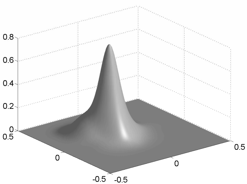
Refer to caption
Refer to caption
Refer to caption
Refer to caption

|ψδ​(t,𝐱)|2|x3=0|\psi^{\delta}(t,\boldsymbol{\rm{x}})|^{2}\big|_{x_{3}=0}, (|φe​(t,𝐱)|2+|φp​(t,𝐱)|2)|x3=0\left(|\varphi_{e}(t,\boldsymbol{\rm{x}})|^{2}+|\varphi_{p}(t,\boldsymbol{\rm{x}})|^{2}\right)\big|_{x_{3}=0}, Vδ​(t,𝐱)|x3=0V^{\delta}(t,\boldsymbol{\rm{x}})\big|_{x_{3}=0} and V⁡(t,𝐱)|x3=0V(t,\boldsymbol{\rm{x}})\big|_{x_{3}=0} at t=0.5.

Refer to caption
Refer to caption
Refer to caption
Refer to caption

|ψδ​(t,𝐱)|2|x3=0|\psi^{\delta}(t,\boldsymbol{\rm{x}})|^{2}\big|_{x_{3}=0}, (|φe​(t,𝐱)|2+|φp​(t,𝐱)|2)|x3=0\left(|\varphi_{e}(t,\boldsymbol{\rm{x}})|^{2}+|\varphi_{p}(t,\boldsymbol{\rm{x}})|^{2}\right)\big|_{x_{3}=0}, Vδ​(t,𝐱)|x3=0V^{\delta}(t,\boldsymbol{\rm{x}})\big|_{x_{3}=0} and V⁡(t,𝐱)|x3=0V(t,\boldsymbol{\rm{x}})\big|_{x_{3}=0} at t=1.0.

Refer to caption
Refer to caption
Refer to caption
Refer to caption

|ψδ​(t,𝐱)|2|x3=0|\psi^{\delta}(t,\boldsymbol{\rm{x}})|^{2}\big|_{x_{3}=0}, (|φe​(t,𝐱)|2+|φp​(t,𝐱)|2)|x3=0\left(|\varphi_{e}(t,\boldsymbol{\rm{x}})|^{2}+|\varphi_{p}(t,\boldsymbol{\rm{x}})|^{2}\right)\big|_{x_{3}=0}, Vδ​(t,𝐱)|x3=0V^{\delta}(t,\boldsymbol{\rm{x}})\big|_{x_{3}=0} and V⁡(t,𝐱)|x3=0V(t,\boldsymbol{\rm{x}})\big|_{x_{3}=0} at t=1.5.

Refer to caption
Refer to caption
Refer to caption
Refer to caption

|ψδ​(t,𝐱)|2|x3=0|\psi^{\delta}(t,\boldsymbol{\rm{x}})|^{2}\big|_{x_{3}=0}, (|φe​(t,𝐱)|2+|φp​(t,𝐱)|2)|x3=0\left(|\varphi_{e}(t,\boldsymbol{\rm{x}})|^{2}+|\varphi_{p}(t,\boldsymbol{\rm{x}})|^{2}\right)\big|_{x_{3}=0}, Vδ​(t,𝐱)|x3=0V^{\delta}(t,\boldsymbol{\rm{x}})\big|_{x_{3}=0} and V⁡(t,𝐱)|x3=0V(t,\boldsymbol{\rm{x}})\big|_{x_{3}=0} at t=2.0.

Figure 14. Numerical results of the density for example 4.2. The first and third column are |ψδ​(t,𝐱)|2|x3=0|\psi^{\delta}(t,\boldsymbol{\rm{x}})|^{2}\big|_{x_{3}=0} and Vδ​(t,𝐱)|x3=0V^{\delta}(t,\boldsymbol{\rm{x}})\big|_{x_{3}=0} for MD system, respectively. The second and fourth column are (|φe​(t,𝐱)|2+|φp​(t,𝐱)|2)|x3=0\left(|\varphi_{e}(t,\boldsymbol{\rm{x}})|^{2}+|\varphi_{p}(t,\boldsymbol{\rm{x}})|^{2}\right)\big|_{x_{3}=0} and V⁡(t,𝐱)|x3=0V(t,\boldsymbol{\rm{x}})\big|_{x_{3}=0} for Schrödinger-Poisson equation, respectively. Here δ=0.01\delta=0.01, △​x=1/64,△​t=1/128\triangle x=1/64,\triangle t=1/128.

5. Conclusion

In this work, we presented a time-splitting spectral scheme for the MD system and similar time-splitting methods for the corresponding asymptotic problems in the (weakly nonlinear) semi-classical and in the non-relativistic regime. The proposed scheme conserves the Lorentz gauge condition, is unconditionally stable and highly efficient as our numerical examples show. In particular, we presented numerical studies for the creation of positronic modes in the semi-classical regime as well as numerical evidence for the smallness of the magnetic fields in the considered non-relativistic scaling. A distinct feature of our time-splitting spectral method, not shared by previous methods (using the time-splitting spectral approach), is that in the non-relativistic limit, the scheme exhibits a uniform convergence in the small parameter δ\delta.

We finally remark that there are several open questions that deserve further exploration. For example, it would be an interesting project to derive a better numerical method for the system of eiconal and transport equations, describing the semi-classical limit, which consequently would allow for a more accurate comparison between the solution of the MD system and limiting WKB-description. A second step then should be the numerical study of the semi-classical MD equations with stronger nonlinearities, in particular 𝒪⁡(1)\mathcal{O}(1)-nonlinearities, a so far completely open problem, even from an analytical point of view.

References

  • [1] W. Bao, S. Jin, P. Markowich, On time-splitting spectral approximations for the Schrödinger equation in the semiclassical regime, J. Comp. Phys. 175 (2002), 487–524.
  • [2] W. Bao, S. Jin, P. Markowich, Numerical study of time-splitting spectral discretizations of nonlinear Schrodinger equations in the semi-classical regimes, SIAM J. Sci. Comput. 25 (2003), no. 1, 27–64.
  • [3] W. Bao, X.G. Li, An efficient and stable numerical method for the Maxwell-Dirac system, J. Comput. Phys. 199 (2004), 663–687.
  • [4] W. Bao and F.F. Sun, Efficient and stable numerical methods for the generalized and vector Zakharov System, SIAM J. Sci. Comput., to appear.
  • [5] W. Bao, F.F. Sun and G.W. Wei, Numerical methods for the generalized Zakharov system, J. Comput. Phys. 190 (2003), no. 1, 201–228.
  • [6] P. Bechouche, N. Mauser, F. Poupaud, (Semi)-nonrelativistic limits of the Dirac equation with time-dependent electromagnetic fields, Comm. Math. Phys. 197 (1998), 405–425.
  • [7] P. Bechouche, N. Mauser, S. Selberg, Nonrelativistic limit of Klein-Gordon-Maxwell to Schrödinger-Poisson, Amer. J. Math. 126 (2004), 31–64.
  • [8] P. Bechouche, N. Mauser, S. Selberg, On the asymptotic analysis of the Dirac-Maxwell system in the nonrelativistic limit, preprint arXiv: math-ap/0303079.
  • [9] J. Bolte, S. Keppeler, A semiclassical approach to the Dirac equation, Ann. Phys. 274 (1999), 125–162.
  • [10] H. Booth, C. Radford, The Dirac-Maxwell Equations with Cylindrical Symmetry, J. Math. Phys. 38 (1997), 4504–4527.
  • [11] J. M. Chadam, Global solutions of the Cauchy problem for the (classical) coupled Maxwell-Dirac equations in one space dimension, J. Funct. Anal. 13 (1973), 173–184.
  • [12] A. Das and D. Kay, A class of exact plane wave solutions of the Maxwell-Dirac equations, J. Math. Phys. 30 (1989), 2280–2284.
  • [13] P. Donat, J. Rauch Dispersive nonlinear geometrical optics, J. Math. Phys. 38 (1997), 1484–1523.
  • [14] M. Esteban, E. Séré, An Overview on linear and nonlinear Dirac equations, Discrete Contin. Dyn. Syst. 8 (2002), no.2, 381–397.
  • [15] M. Flato, J. C. H. Simon, E. Tafflin, Asymptotic Completeness, Global Existence and the Infrared Problem for the Maxwell-Dirac Equation, Memoirs of the AMS no. 127 (1997).
  • [16] L. Gross, The Cauchy problem for the coupled Maxwell and Dirac equations, Comm. Pure Appl. Math. 19 (1966), 1–15.
  • [17] S. Jin, Z. Xin, Numerical passage from systems of conservation laws to Hamilton-Jacobi equations, and a relaxation scheme, SIAM J. Num. Anal. 35 (1998), 2385–2404.
  • [18] S. Jin, P. Markowich, and C. Zheng, Numerical simulation of a generalized Zakharov system, J. Comput. Phys. 201 (2004), 376-395.
  • [19] M. Masmoudi, N. Mauser, The self-consistent Pauli equation, Monatsh. Math. 132 (2001), no. 6, 759–763.
  • [20] B. Najman, The nonrelativistic limit of the nolinear Dirac equation, Ann. Inst. H. Poincare, Anal. Non Lineaire 9 (1992) 3–12.
  • [21] J. Rauch, Lectures on Nonlinear Geometrical Optics, IAS/Park City Math. Series 5, AMS (1999).
  • [22] F. Schwabl, Advanced Quantum Mechanics, Springer (1999).
  • [23] C. Sparber and P. Markowich, Semiclassical asymptotics for the Maxwell-Dirac system, J. Math. Phys. 44 (2003), no. 10, 4555–4572.
  • [24] C. Sparber and P. Markowich, Erratum: Semiclassical asymptotics for the Maxwell-Dirac system, to appear in J. Math. Phys. 45 (2004), no 12.
  • [25] S. Teufel, Adiabatic perturbation theory in quantum dynamics, Lecture Notes in Math. 1821, Springer 2003.
  • [26] H. Spohn, Semiclassical limit of the Dirac equation and spin precession, Ann. Physics 282 (2000), no. 2, 420–431.