Lattice baryons in the expansion
Abstract
Results are presented for hadron spectroscopy with gauge groups with , 5, 7. Calculations use the quenched approximation. Lattice spacings are matched using the static potential. Meson spectra show independence on and vacuum-to-hadron matrix elements scale as . The baryon spectrum shows the excitation levels of a rigid rotor.
I Introduction
Replacing the “3” of color by “N”” and then taking N to infinity has a long history in the (continuum) phenomenology of the strong interactions, dating back to Refs. [1, 2].
There is also a literature of lattice simulations applied to gauge theories with the group , for moderately large . Most of it [3, 4, 5, 6, 7, 8] is directed at the properties of pure gauge theory. I know of two papers on meson spectroscopy: Refs. [9, 10]. They are done at smaller values of “large ,” , 3, 4, 6. They are pretty standard lattice QCD spectroscopy calculations and reveal the N-independence of meson masses. Narayanan, Neuberger, and collaborators [11, 12] have measured masses and the pseudoscalar decay constant from simulations at much larger (exploiting reduction, to simulate on smaller lattice sizes).
But only Ref. [13] discusses large-N expectations for baryons, and it only makes comparisons to actual lattice data for . So it seemed like an appropriate time to look at a lattice calculation of baryon spectroscopy at several values of .
Baryons in large N seem to be fascinating objects, either viewed as many-quark states [14] or as topological objects in effective theories of mesons[15, 16]. There is an enormous (continuum) literature about spectroscopy and matrix elements for large baryons. Assorted early references include [17, 18, 19, 20, 21], summarized in a review, Ref. [22]. Perhaps a lattice study might reveal something interesting?
In fact, it does: general arguments [16, 17] state that the mass of an color baryon of angular momentum should show a rotor spectrum:
| (1) |
The formula applies to baryons made of an isospin doublet of equal mass quarks. The parameters and depend on the quark mass and both should be some “typical hadron size,” a few hundred MeV. The observation of Eq. 1 in simulation data is the main new result of this paper. Common expectations are that Eq. 1 is only true for small values of , because then the terms have meaning as a good expansion in . However, I observe that it holds both for the bottom and the top of the multiplets where I did measurements.
The first response of the lattice simulator to a proposal to look at baryons at large is undoubtedly negative: The cost of an -color simulation scales roughly like , just from the cost of multiplying matrices. Baryons are large objects so big volumes will be needed. Ordinary () baryon correlators are noisy and because baryon masses scale as , baryons in higher are probably noisier. And most of the literature involves some combination of small effects and expectation values of operators (), which are already hard enough for [23]. Fortunately, large tests seem (mostly) not to require extrapolations to zero quark mass.
Only for odd are baryons fermions, of course, so I am performing simulations of gauge theories with , 5, 7.
I used the quenched approximation for all . That means that, truly, I am not simulating QCD for any value of . However, a first study does not quite demand the same level of quality as a later one might. I am interested in comparing simple observables in systems which differ only in , but otherwise have the same UV cutoff (lattice spacing), lattice action, and physical volume. This is easy to set up in quenched approximation.
Of course, the system which is simulated ought to have some connection to the real world. It is easy to justify a quenched approximation for large (although one could argue that it remains an open question, whether such justification is correct). Quenched simulations for are obsolete, but the effects of dynamical fermions on spectroscopy are really not all that large: away from the deep chiral limit they are small, order ten per cent for simple observables (compare Fig. 1 in Ref. [24]).
The difficulty with using the quenched approximation comes when one wishes to convert a lattice number to MeV. The spectrum of quenched QCD is simply different from the spectrum of “real” QCD. I will compare dimensionless ratios of lattice quantities in my tests of scaling with . Any conversions to MeV I make are only qualitative statements.
One could take the position that one should test everything about large- QCD at once, by doing simulations with dynamical fermions at several values of . This just postpones the matching problem: the spectrum of the different QCD’s will be different. But perhaps that is not the right point of view. The real question one asks when comparing several values of is whether dimensionless ratios of masses show some smooth behavior with . And for that, one can begin simply, make observations, and then ask how they change as one does ever more realistic simulations.
For all ’s, I use lattices of size points. I match the bare couplings so that the lattice spacings, as measured by various observables from the heavy quark potential, are the same, and then sweep in quark mass over similar ranges. This insures that finite volume and nonzero lattice spacing lattice artifacts will be similar across the board. I set the common scale using the shorter version of the Sommer [25] parameter, , defined in terms of the force so that at . The real-world value is fm [26], and with it my lattice spacings would be about 0.08 fm.
Before going on, it’s useful to set some definitions. The ’t Hooft coupling is
| (2) |
and the usual gauge coupling is thus
| (3) |
The combination , which appears in all perturbative calculations of renormalization factors, is equal to . For comparisons at fixed ’t Hooft coupling, like the ones I present, this suggests that differences which might be perturbative (lattice–to–continuum matching factors, for example) will scale up to corrections of order .
The outline of the paper is as follows: The next section describes some technical problems I faced: using fat links, gauge fixing, and the construction of baryon operators. Only the third topic might be of interest to continuum physicists. Next, I present lattice results for the potential and for meson masses and simple matrix elements. The potential measurements show the extent to which lattice spacings are matched. The mesonic observables illustrate the – independence of masses and the scaling of quantities like the pseudoscalar decay constant. Finally, in Section IV, I show some results for baryon spectra. The major one is the presence of a rotor spectrum of excitations for two-flavor baryons.
II Technical details
II.1 Simulation techniques
My simulations use a version of the publicly available package of the MILC collaboration [27], modified to generate gauge configurations and quark propagators at arbitrary . Prior to this project, it had been extensively used in studies of , 3, 4 [28] .
The gauge action is the usual Wilson action. Quenched simulations are performed using the standard mix of Brown - Woch microcanonical over-relaxation [29] and Cabibbo - Marinari heat bath updates [30], performed on all subgroups of the link variables. It is known that simulations performed on subgroups suffer critical slowing down at larger , but the largest is only 7 and this problem did not appear. Lattices are spaced 100 sweeps of the lattice apart, for later analysis.
The spectroscopy was intended to be a typical lattice QCD calculation writ large. This involved an improved fermion action and extended sources for hadronic correlation functions. To achieve these goals a number of small technical problems had to be solved. Many of them have been encountered in other large- studies, but perhaps my solutions are a bit different than what is found there, and might be worth reporting.
II.2 fat links; gauge fixing
My lattice fermions are clover fermions with normalized hypercubic (nHYP-link) smeared links as their gauge connections[31]. The clover coefficient is fixed at its tree level value, . This particular discretization is known to work well, with small scaling violations, in both ordinary QCD phenomenology and in beyond-Standard Model studies in , , . So the first technical problem is the construction of the nHYP link for arbitrary . To describe the nHYP link in words, it is a local average of gauge connections over the hypercubes surrounding the link, which smears out the gauge field for the fermion. The specific problem to be solved is that the the fat link is the average of a set of paths which produces a sum of matrices, call it . The fat link is defined as
| (4) |
This is the matrix which maximizes . The quantity is computed using the Cayley - Hamilton theorem as described in Appendix B of Ref. [32]. This construction involves finding the eigenvalues of , which is done using a Jacobi algorithm.
As written, is an element of , not . This is not an issue when it is used for the fermions since all that we care about is that our action should be gauge invariant, and under a gauge transformation both the thin and fat links transform the same way.
State of the art spectroscopic calculations use extended sources as interpolating fields for hadrons. In this work configuration of link variables is gauge fixed to lattice Coulomb gauge and the source for the quark propagator is some spatially extended function. So, we need to gauge fix our lattices to lattice Coulomb gauge, rotating the links to maximize , labeling the spatial directions. This is done by finding a matrix at each site of the lattice which maximizes where is the sum of forward going ’s emanating from minus the sum of ’s terminating on site .
In the author’s code, gauge fixing is done iteratively by sweeping through the lattice and, site by site, determining an optimal by maximizing . As in the case of configuration generation, the relaxation is done using the subgroups of . Unfortunately, for relaxing on the subgroups suffers critical slowing down and it becomes impossible to carry out gauge fixing without performing an enormous number of iterations.
This is a variation of a problem which has been previously observed (and solved) by several groups simulating large gauge theories, with [33, 34]. There the problem is in the update step. Updating on subgroups produces a simulation algorithm with a long autocorrelation time, which becomes longer with increasing . The solution is to perform over-relaxation on the full group, implementing an old idea of Creutz [35]. I do this a little differently than Refs. [33, 34]. The maximizing is given by Eq, 4, which I have already dealt with while generating the fat links for the fermion action. The same application of the Cayley-Hamilton theorem gives . As I already remarked, this is an element of , not . Now one needs elements, so I must compute the determinant of , extracting its phase and performing an additional multiplication by the diagonal matrix . Doing this makes gauge fixing no more expensive for than for .
II.3 Baryon operators
Mesonic states are constructed in the usual way, by sandwiching fermion propagators with Dirac matrices. Baryons are a bit more complicated. In it is common to use relativistic sources (, for example, for the proton). I don’t know a nice way to generalize this to , so I built baryon states using non-relativistic quark model states. So far, I have only considered flavors of quarks. In what follows, I will label the flavors as and , although one can give them different masses – in the same operator can give the or , for example.
In the MILC code, quark propagators are constructed in the Weyl ( diagonal) basis, and are rotated to basis. I keep the two “large” components of the propagator’s source and sink spin indices to be the fields which contract the quark model states. There are two choices for projection (eigenvalues of allow forward going in time and backward going two-component quark propagators). One projection has the lightest positive parity state in a channel as the forward-going state, and the lightest negative-parity state as the backward-going one. The situation is reversed for the other projector. In order to reduce noise, these two propagators are summed (actually subtracted), configuration by configuration. This produces a single correlator extending halfway across the lattice, which is a candidate for fitting to a single dying exponential.
A generic color baryon operator can be written as
| (5) |
The ’s are an appropriate set of Clebsch-Gordon coefficients. The baryon propagator is a multiple sum over source and sink colors and spin coefficients of products of quark propagators. This creates the possibility a large number of terms. Fortunately, many are redundant.
I condense states as follows. (I suspect that this is quite inefficient and that more efficiency is almost certainly possible.) I begin with states of definite and content. These states are eigenstates of , , and . I then anticommute fermion fields into a “standard order,” shown in Eq. 5: moving from the left, spin-up quarks, spin-down quarks, spin-up quarks, and spin-down quarks. The epsilon symbol absorbs the resulting minus signs.
Then, two examples are the state
| (6) |
and the proton operator
| (7) |
Wick’s theorem says that the quark propagator itself is also a determinant:
( is a permutation of indices). The baryon propagator, then is a product of an up-quark determinant times a down quark determinant, summed over all the color combinations of the individual up and down quarks. Many terms are redundant in this product, as can be seen in an example, the proton: The contributions from the source terms are antisymmetric in both Eqs. 5 and . This means that it is only necessary to keep one color ordering , for example) for each pair of colors in the baryon propagator, and each term can be reweighted by a factor of . This generalizes straightforwardly so that a a term in any wave function with spin-up quarks, spin-down quarks, spin-up quarks, spin-down quarks, picks up a restricted color sum, a single color ordering for each individual spin-flavor label and a multiplicity .
An extreme example of this pruning procedure is the the propagator for the state of Eq. 6. It is
| (9) |
where is the matrix of propagators from a source color to a sink one.
The lower the , the more complicated are the wave functions. By , the states involve several hundred color combinations per spin configuration. This is getting quite unwieldy. (Since the nonrelativistic quark propagator is itself only a matrix, there must be more redundancy!) But for now, I go on, naively.
To summarize, flavor wave functions and propagators for the various states are
- •
: as already described, there is one determinant of an matrix, for a cost .
- •
Analogs of and states are
(10) The baryon correlator is built of terms, one for each color in the source and sink. Each is a determinant of an matrix – the propagator of the up quarks.
- •
: We have an matrix of quark propagators and color terms in the interpolating field for a cost of roughly :
(11) - •
: An matrix of propagators. The last term in the interpolating field has about color possibilities, for a cost of .
- •
: our lowest state if ; there are terms to evaluate.
Still to be constructed are three flavor (, , ) states.
An obvious solution to the problem of increasing multiplicity is to prune states by doing an incomplete color sum. This will collide with another big problem: baryon signals degrade as increases. For now, the only way to fight this is to collect larger data sets. Along the way, however, one can try to improve our signals by tactics such as averaging over the propagators with the same and different ’s. (In practice, I combine the and propagators into a single correlator.) Another approach involves forcing a fit of several correlators which couple to the same states to a common mass. Ultimately, a variational calculation along the lines of what is done for excited state baryon spectroscopy might be necessary.
III Results for pure gauge and mesonic observables
I present quenched results from three ’s, , 5, 7. I have data sets of 80, 120, and 160 propagators, respectively The bare gauge coupling is tuned to match potentials through the Sommer parameters or . (Recall . is the shorter-distance version of the Sommer parameter, . In the real world, fm.)
In the present simulations, (to match to previous work by Ref. [10]), and then the and 7 couplings were tuned to match . Couplings and derived quantities are recorded in Table 1. The bare t Hooft couplings turn out to be quite similar. Wilson-action simulations for have a first order lattice-artifact transition, and I checked that my simulations are above it. Potentials for the three values of N are shown in Fig. 1. They seem satisfactorily matched.
The combination or ( is the string tension) gives a dimensionless combination of the Sommer radius and the string tension . The table shows that this quantity scales well.

My spectroscopy is based on smeared Gaussian sources and point sinks. At each I collected sets for several different values of the width of for the source. These correlation functions are not variational since the source and sink are different. Thus, as is varied, the effective mass ( is defined through fitting correlators at a single distance to a single exponential; with open boundary conditions for correlator , ) can approach its asymptotic value from above or below. I observe that typically, as rises, the mixed Gaussian - point correlators make their approach from above for smaller , and from below for bigger . An example of this behavior is shown in Fig. 2. (At large , the signal deteriorates – a characteristic feature quite familiar from many studies. The noise is enhanced by the small data sets – 40 lattices – used to make the figure.) Then, rather than re-running the propagator code with yet another source, I can combine pairs of sources to produce a flat distribution using say
| (14) |
For , the optimal source is a linear combination of and 6 sources, favoring larger as the quark mass falls. For I mix sources with and 8. For the source produced flat effective mass plots across my mass range, and I did not do any source mixing.
Tables 2-4 contain the resulting spectroscopy. The values of the masses are highly correlated because they come from the same underlying configurations. Mass differences, which will be described below, are taken from jackknife averages of the data.

Now I turn to results for mesonic observables. The critical hopping parameter is determined through the vanishing point for the Axial Ward Identity (AWI) quark mass, defined as
| (15) |
where the axial current , the pseudoscalar density , and could be any source. Here it is my Gaussian shell model source.
The mass is shifted from its free value in the usual way. To compare to usual expectations, recall the relation between and : we expect that the mass shift
| (16) |
to show variation. This I roughly see; compare Fig. 3. Just for comparison over a wider range, I show the older results of Ref. [9], done with unimproved Wilson fermions.

Next, we turn to spectroscopy, shown for mesons in Fig. 4 and baryons in Fig. 5. Data are plotted in terms of the AWI quark mass, in units of , to make the -axis the same for all . The near independence of meson masses on N (when expressed in terms of a common variable) is apparent. Not so, for baryons!


One is tempted to compare the chiral limit of the vector meson mass as a function of . A simple linear fit to the data of Fig. 4 gives , 1.44(1) and 1.52(1) for , 5, 7. With a nominal MeV, this is about 900 MeV to 1 GeV versus 770 MeV for the physical rho meson. One always has to be careful with quenched lattice results from a single volume and lattice spacing, but the number is completely sensible. It is close to the results of Refs. [9, 10].
(Using completely different methodology plus a different choice of physical input to set the lattice scale, the authors of Ref. [12] have a mass which is from thirty per cent to a factor of two higher than this. The difference between their result and the low-N ones will probably only be resolved by removing the many differences in methodology one at at time.)
In what follows, I will replace the quark mass as the independent variable by the square of the ratio of the pseudoscalar to vector meson mass. The quark mass is scheme dependent. Of course, nothing I say is affected by this choice.
Vacuum-to-meson matrix elements are expected to scale as . I have looked at the pseudoscalar, vector meson, and axial vector meson decay constants. To be explicit, they are defined as follows:
| (17) |
(so MeV) while the vector meson decay constant of state is defined as
| (18) |
and the axial vector meson decay constant of state is
| (19) |
is a unit polarization vector. The lattice quantities are converted to continuum convention by . I have left out the lattice-to-continuum Z-factor. With nHYP clover fermions, it is a few percent away from unity.
The pseudoscalar decay constant is shown in Fig. 6. I show the dimensionless combination . It’s nice to see the scaling. Naive linear extrapolations give , 0.151(1) and 0.154(2) for , 5, 7. The real world value is fm MeV , so the quenched decay constant at this lattice spacing is coming in about 15 per cent high. Experts know that this kind of extrapolation is far too naive, to say nothing about comparing quenched QCD to the real world. Nevertheless, the answer is not absurd. Ref. [24] shows a figure of with the ratio of quenched to its experimental result about ten per cent high.
scaling for the pseudoscalar decay constant was first observed by the authors of Ref. [11]. Their numerical result for the decay constant, translated to , is also high, but by 40 per cent. Detecting the origin of this difference will probably again require detailed numerical work.
The same comparison is shown for , and in Fig. 7. The decay constant is quite noisy at small quark mass and I omit those results as untrustworthy. The scaling rule works well here, too.


IV Results for baryons – the rotor spectrum
My baryon data in Fig. 5 shows masses which increase roughly linearly in . All data shows that for the baryons, higher does lie higher in energy. This is no surprise, so let’s look deeper. Fig. 8 shows the splitting between the various members of each multiplet. It is extracted using a jackknife average of differences of the two baryon masses.

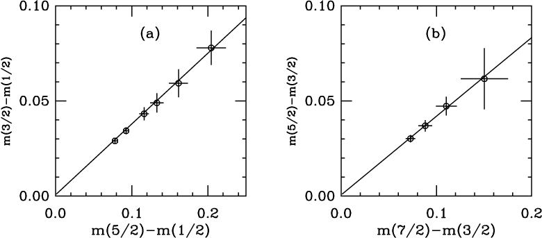
I now demonstrate that the masses in Fig. 8 form a rotor spectrum. First, we can test the numerator of the rotor term of Eq. 1 by . This is done by looking at the ratio differences
| (20) |
for which the constants (, ) cancel. The result is shown in Fig. 9. I just plot one mass difference as a function of the other one and compare the data to a straight line of zero intercept whose slope is given by Eq. 20. The rotor spectrum is confirmed for all the members of the and 7 multiplets I observe.
Second, one can look at the splitting, and check the dependence for the bottom of the multiplets:
| (21) |
Given the states I have recorded, this can only be done for and 5. Rescaling the mass difference by exposes . The result is shown in Fig. 10(a). This is quite promising: the and 5 data coincide.

Next, we can look at the top of the multiplet. Eq. 1 gives us a rescaled Landé interval rule: it says that the splitting between the and states is a constant, , independent of . Fig. 10(b) shows this difference. It and panel (a) share the common points, but the other points are different. The envelope of the curve is .
By design, these differences ignore the term in Eq. 1. To get it, we can look at the top of the multiplets,
| (22) |
or the bottom of the multiplets,
| (23) |
Fig. 11 shows these two mass formulas. Again, they behave consistently.

Figs. 10 and 11 show that the and coefficients in Eq. 1 have typical hadronic sizes. Inserting a nominal lattice spacing, MeV, we see that MeV at small quark mass and is an increasing function of quark mass. In quark model language, is the constituent quark mass, and its value and dependence on quark mass are both quite reasonable. MeV and falls with energy. Again this is a typical hadronic scale.
These values address an old conundrum of large- phenomenology: the mass difference of the nucleon and is supposed to be order . It is measured to be about 300 MeV, which is itself order . The plots of mass differences show that the nucleon- mass splitting is indeed well-described by large- QCD. Having data at several ’s as well as at several quark masses makes this result appear immediately.
V Conclusions
The qualitative features of large - QCD phenomenology are easy to observe. The shape of the potential (characterized by the scaling combination ) is - independent. Meson masses show little dependence – is -independent. Vacuum - to -hadron matrix elements scale as . Two-flavor baryons show a prominent rotor spectrum. This seems to be true for both the bottom of the spectrum (low ) and the top ( states).
Naively, one might expect that the wave function of the baryon would be - independent. Lattice simulations do not generally directly reveal wave function information, but one might expect that the same interpolating fields might behave the same for different ’s. That does not seem to be the case; larger seems to prefer larger Gaussian trial wave functions. But perhaps even is not such large and one should push farther.
Readers who do lattice simulations can undoubtedly list many obvious extensions of this project: smaller lattice spacing, to do an honest extrapolation to the continuum limit, bigger volumes to check that the answers are trustworthy, smaller quark masses, and bigger ’s are obvious technical improvements. Giving the two fermions different masses, or better yet, considering flavor , would allow more tests of large- spectroscopy. One might really want to test whether dynamical fermions become less important at large . Writing the code to simulate fundamental fermions is straightforward; running it might be costly, and seeing the expected small differences shrink as rises would be even more costly.
The continuum literature of large - N baryons is more than thirty years old, and I clearly have only scratched its surface in this paper. Several simple ingredients were useful: having data at several ’s, at several ’s for each , and having data at many quark masses. Most of the continuum literature I have read restricts itself to statements about and 3/2 – presumably because that is all that exists in experimental data. Predictions for any can challenge the lattice and would be candidates for future studies.
| 6.0175 | 17.5 | 34.9 | |
| 2.99 | 2.86 | 2.81 | |
| 5.36(6) | 5.20(5) | 5.41(3) | |
| 3.90(3) | 3.77(3) | 3.91(2) | |
| 1.175(3) | 1.172(3) | 1.167(2) | |
| 0.856(5) | 0.850(4) | 0.845(2) |
| 0.1230 | 0.119 | 0.525(2) | 0.617(3) | 0.996(6) | 0.942(5) |
| 0.1240 | 0.089 | 0.449(2) | 0.561(3) | 0.915(7) | 0.846(5) |
| 0.1250 | 0.055 | 0.362(2) | 0.505(4) | 0.835(8) | 0.744(6) |
| 0.1253 | 0.046 | 0.333(2) | 0.491(5) | 0.804(9) | 0.700(6) |
| 0.1260 | 0.029 | 0.255(3) | 0.457(6) | 0.747(12) | 0.613(7) |
| 0.1265 | 0.014 | 0.184(4) | 0.427(10) | 0.703(13) | 0.516(12) |
| 0.1240 | 0.127 | 0.565(1) | 0.655(1) | 1.864(6) | 1.814(5) | 1.786(5) |
| 0.1250 | 0.099 | 0.488(1) | 0.593(1) | 1.708(6) | 1.650(6) | 1.616(5) |
| 0.1260 | 0.070 | 0.403(1) | 0.532(2) | 1.566(7) | 1.488(6) | 1.446(6) |
| 0.1265 | 0.055 | 0.356(1) | 0.500(2) | 1.486(7) | 1.404(6) | 1.356(6) |
| 0.1270 | 0.041 | 0.302(2) | 0.469(3) | 1.419(8) | 1.325(7) | 1.270(7) |
| 0.1275 | 0.026 | 0.240(2) | 0.440(4) | 1.357(10) | 1.243(9) | 1.177(8) |
| 0.1260 | 0.115 | 0.565(1) | 0.663(1) | 2.681(11) | 2.649(8) | 2.612(8) |
| 0.1270 | 0.088 | 0.488(1) | 0.603(1) | 2.483(9) | 2.420(10) | 2.386(9) |
| 0.1280 | 0.062 | 0.401(1) | 0.537(2) | 2.279(11) | 2.215(11) | 2.174(10) |
| 0.1290 | 0.036 | 0.299(1) | 0.471(3) | 2.082(15) | 1.994(12) | 1.929(11) |
Acknowledgements.
This project began as a direct result of my participation in the Workshop on Large-N Gauge Theories at the Galileo Galilei Institute in Florence in May 2011. I thank C. DeTar, R. Lebed, A. Manohar, H. Neuberger, and M. Teper for discussions about this subject. The modification of the MILC code to arbitrary number of colors was done with Y. Shamir and B. Svetitsky. This work was supported in part by the U. S. Department of Energy.References
- [1] G. ’t Hooft, Nucl. Phys. B 72, 461 (1974).
- [2] G. ’t Hooft, Nucl. Phys. B 75, 461 (1974).
- [3] B. Lucini, M. Teper, U. Wenger, JHEP 0502, 033 (2005). [hep-lat/0502003].
- [4] B. Lucini, M. Teper, U. Wenger, JHEP 0406, 012 (2004). [hep-lat/0404008].
- [5] B. Lucini, M. Teper, U. Wenger, Nucl. Phys. B715, 461-482 (2005). [hep-lat/0401028].
- [6] B. Lucini, M. Teper, U. Wenger, JHEP 0401, 061 (2004). [hep-lat/0307017].
- [7] B. Lucini, M. Teper, U. Wenger, Phys. Lett. B545, 197-206 (2002). [hep-lat/0206029].
- [8] B. Lucini, A. Rago and E. Rinaldi, arXiv:1202.6684 [hep-lat].
- [9] L. Del Debbio, B. Lucini, A. Patella, C. Pica, JHEP 0803, 062 (2008). [arXiv:0712.3036 [hep-th]].
- [10] G. S. Bali, F. Bursa, JHEP 0809, 110 (2008). [arXiv:0806.2278 [hep-lat]].
- [11] R. Narayanan and H. Neuberger, Phys. Lett. B 616, 76 (2005) [arXiv:hep-lat/0503033].
- [12] A. Hietanen, R. Narayanan, R. Patel and C. Prays, Phys. Lett. B 674, 80 (2009) [arXiv:0901.3752 [hep-lat]].
- [13] E. E. Jenkins, A. V. Manohar, J. W. Negele, A. Walker-Loud, Phys. Rev. D81, 014502 (2010). [arXiv:0907.0529 [hep-lat]].
- [14] E. Witten, Nucl. Phys. B160, 57 (1979).
- [15] E. Witten, Nucl. Phys. B 223, 433 (1983).
- [16] G. S. Adkins, C. R. Nappi and E. Witten, Nucl. Phys. B 228, 552 (1983).
- [17] E. E. Jenkins, Phys. Lett. B315, 441-446 (1993). [hep-ph/9307244].
- [18] R. F. Dashen, E. E. Jenkins, A. V. Manohar, Phys. Rev. D49, 4713 (1994). [hep-ph/9310379].
- [19] R. F. Dashen, E. E. Jenkins, A. V. Manohar, Phys. Rev. D51, 3697-3727 (1995). [hep-ph/9411234].
- [20] E. E. Jenkins, R. F. Lebed, Phys. Rev. D52, 282-294 (1995). [hep-ph/9502227].
- [21] J. Dai, R. F. Dashen, E. E. Jenkins, A. V. Manohar, Phys. Rev. D53, 273-282 (1996). [hep-ph/9506273].
- [22] A. V. Manohar, “Large N QCD,” hep-ph/9802419.
- [23] For a recent appraisal, see H. Wittig, “Low-energy particle physics and chiral extrapolations,” arXiv:1201.4774 [hep-lat].
- [24] C. T. H. Davies et al. [HPQCD and UKQCD and MILC and Fermilab Lattice Collaborations], Phys. Rev. Lett. 92, 022001 (2004) [hep-lat/0304004].
- [25] R. Sommer, Nucl. Phys. B 411, 839 (1994) [arXiv:hep-lat/9310022].
- [26] A. Bazavov, D. Toussaint, C. Bernard, J. Laiho, C. DeTar, L. Levkova, M. B. Oktay and S. Gottlieb et al., Rev. Mod. Phys. 82, 1349 (2010) [arXiv:0903.3598 [hep-lat]].
- [27] http://www.physics.utah.edu/%7Edetar/milc/
- [28] T. DeGrand, Y. Shamir and B. Svetitsky, Phys. Rev. D 83, 074507 (2011) [arXiv:1102.2843 [hep-lat]]; Phys. Rev. D 82, 054503 (2010) [arXiv:1006.0707 [hep-lat]]; arXiv:1202.2675 [hep-lat].
- [29] F. R. Brown, T. J. Woch, Phys. Rev. Lett. 58, 2394 (1987).
- [30] N. Cabibbo, E. Marinari, Phys. Lett. B119, 387-390 (1982).
- [31] A. Hasenfratz, R. Hoffmann, S. Schaefer, JHEP 0705, 029 (2007). [hep-lat/0702028].
- [32] T. DeGrand, Y. Shamir and B. Svetitsky, arXiv:1202.2675 [hep-lat].
- [33] J. Kiskis, R. Narayanan, H. Neuberger, Phys. Lett. B574, 65-74 (2003). [hep-lat/0308033].
- [34] P. de Forcrand, O. Jahn, [hep-lat/0503041].
- [35] M. Creutz, Phys. Rev. D36, 515 (1987).